Structure recovery for partially observed discrete Markov random fields on graphs under not necessarily positive distributions

Abstract

We propose a penalized pseudo-likelihood criterion to estimate the graph of conditional dependencies in a discrete Markov random field that can be partially observed. We prove the convergence of the estimator in the case of a finite or countable infinite set of nodes. In the finite case the underlying graph can be recovered with probability one, while in the countable infinite case we can recover any finite sub-graph with probability one, by allowing the candidate neighborhoods to grow as a function $o(\log n)$, with $n$ the sample size. Our method requires minimal assumptions on the probability distribution and contrary to other approaches in the literature, the usual positivity condition is not needed. We evaluate the performance of the estimator on simulated data and we apply the methodology to a real dataset of stock index markets in different countries.

1 Introduction

Discrete Markov random fields on graphs, usually called graphical models in the statistical literature, have received much attention from researchers in recent years, especially due to their flexibility to capture conditional dependence relationships between variables [13, 11, 15, 20, 4]. They have been applied to many different problems in different fields such as Biology [24], Social Sciences [25] or Neuroscience [5]. Graphical models are in some sense “finite” versions of general random fields or Gibbs distributions, classical models in stochastic processes and statistical mechanics theory [8].

In this work we focus on discrete Markov random field models (with a finite or countable infinite set of variables), where the set of random variables takes values on a finite alphabet. One of the main statistical questions for this type of models is how to recover the underlying graph; that is, the graph determined by the conditional dependence relationships between the variables. For the class of Markov random fields on lattices some methods based on penalized pseudo-likelihood criteria like the Bayesian Information Criterion (BIC) of [23] have appeared in the literature [3], see also [26, 17]. On the case of Markov random fields defined on general graphs the most studied model is the binary graphical model with pairwise interactions where structure estimation can be addressed by using standard logistic regression techniques [25, 21], distance based approaches between conditional probabilities [6, 2] and maximization of the $\ell^{1}$-penalized pseudo-likelihood [1, 10], see also [22]. In the case of bigger discrete alphabets or general type of interactions, to our knowledge the only work addressing the structure estimation problem is [18], where the authors obtain a characterization of the edges in the graph with the zeros in a generalized inverse covariance matrix. Then, this characterization is used to derive estimators for restricted classes of models and the authors prove the consistency in probability of these estimators.

Markov random fields have also been proposed for continuous random variables, where the structure estimation problem has been addressed by $\ell_{1}$ regularization for Gaussian Markov random fields [19] and also extended to non-parametric models [12, 16] and general conditional distributions from the exponential family [27].

All these works, for discrete or continuous random variables, assume the model satisfies a usual “positivity” condition, that states that the probability distributions of finite sub-sets of variables are strictly positive. The positivity condition guarantees a factorization property of the joint distribution, thanks to a classical result known as Hammersley-Clifford theorem [9]. But the positivity condition seem to be extremely strong for discrete distributions, where in many applications some configurations are impossible to occur and then have zero probability. Moreover, the positivity condition does not enable to consider “sparse” models, where many parameters are assumed to be zero. These models are specially appealing for high dimensional data, where the number of variables is high and the number of relevant parameters in the model must be assumed relatively small in order to have efficient estimators.

In this work we address the structure estimation problem for discrete Markov random fields without assuming the positivity condition. We first introduce a penalized pseudo-likelihood criterion to estimate the neighborhood of a node, that is later combined to obtain an estimator of the underlying graph. We prove that both estimators converge almost surely to the true underlying graph in the case of a finite graphical model when the sample size grows, without imposing additional hypothesis on the model. In the countable infinite case, that is when the underlying graph is infinite and the number of observed variables is allowed to grow with the sample size, we prove that the estimator restricted to a finite sub-graph also converges almost surely to the corresponding sub-graph.

The paper is organized as follows. Section 2 presents the definition of the model, including some examples. Section 3 introduces the different estimators of the conditional dependence graph and presents the statements proofs of the main consistency results. Finally, in Section 4 we evaluate the estimators performance through simulations, in Section 5 we show a real data application and in the Appendix we present the proofs of some auxiliary results.

2 Discrete Markov random fields on graphs

A graph is a pair $G=(V,E)$, where $V$ is the set of vertices (or nodes) and $E$ is the set of edges, $E\subset V\times V$. A graph $G$ is said simple if for all $i\in V$, $(i,i)\not\in E$ and it is said undirected if $(i,j)\in E$ implies $(j,i)\in E$ for every pair $(i,j)\in V\times V$. Given any set $S$, the symbol $|S|$ denotes its cardinality.

Let $A$ be a finite set, a random field on $A^{V}$ is a family of random variables indexed by the elements of $V$, $\{X_{v}:v\in V\}$, where each $X_{v}$ is a random variable with values in $A$. For $\Delta\subseteq V$, a subset of vertices, we write $X_{\Delta}=\{X_{i}\colon i\in\Delta\}$, and $a_{\Delta}=\{a_{i}\in A\colon i\in\Delta\}$ denotes a configuration on $\Delta$. The law (joint distribution) of the random variables $X_{V}$ is denoted by $\mathbb{P}$.

For any finite $\Delta\subset V$ we write

$$p(a_{\Delta})=\mathbb{P}(X_{\Delta}=a_{\Delta})\;\mbox{ with }a_{\Delta}\in A^{\Delta}$$ (1)

and if $p(a_{\Delta})>0$ we denote by

$$p(a_{\Phi}|a_{\Delta})=\mathbb{P}(X_{\Phi}=a_{\Phi}|X_{\Delta}=a_{\Delta})\;\mbox{ for }a_{\Phi}\in A^{\Phi},\,a_{\Delta}\in A^{\Delta}$$ (2)

the corresponding conditional probability distributions.

Given $v\in V$, a neighborhood $W$ of $v$ is any finite set of vertices with $v\notin W$. If there is a neighborhood $W$ of $v$ satisfying

$$p(a_{v}|a_{W})\;=\;p(a_{v}|a_{\Delta})$$ (3)

for all finite $\Delta\supset W,\,v\notin\Delta$ and all $a_{v}\in A,a_{\Delta}\in A^{\Delta}$ with $p(a_{\Delta})>0$, then $W$ is called Markov neighborhood of $v$. The definition of a Markov neighborhood $W$ is equivalent to request that for all $\Phi$ finite (not containing $v$) with $\Phi\cap W=\emptyset$, $X_{\Phi}$ is conditionally independent of $X_{v}$, given $X_{W}$. Formally,

$$X_{v}\!\perp\!\!\!\perp\!X_{\Phi}|X_{W}\,,\,\mbox{ for all }\Phi\mbox{ with }\Phi\cap W=\emptyset,$$ (4)

where $\!\perp\!\!\!\perp\!$ is the usual symbol denoting independence of random variables. This conditionally independence assumption defining the Markov neighborhoods corresponds to the property known as local Markov in finite graphical models, that is weaker than the usually assumed global Markov property, see [13] for details.

A basic fact that we can derive from the definition is that if $W$ is a Markov neighborhood of $v\in V$, then any finite set $\Delta\supset W$ is also a Markov neighborhood of $v$. On the other hand, if $W_{1}$ and $W_{2}$ are Markov neighborhoods of $v$ then it is not always true in general that $W_{1}\cap W_{2}$ is a Markov neighborhood, as shown in the following example.

Example 2.1.

Let $V=\{1,2,3\}$ and consider the vector $(X_{1},X_{2},X_{3})$ of Bernoulli random variables with $\mathbb{P}(X_{i}=0)=1/2$, $\mathbb{P}(X_{i}=1)=1/2$, for $i=1,2,3$. Suppose that $X_{1}=X_{2}=X_{3}$ with probability 1. Then it is easy to check that both $\{2\}$ and $\{3\}$ are Markov neighborhoods of node $1$, but the intersection is not a Markov neighborhood (which will imply $X_{1}$ being independent of $X_{2}$ and $X_{3}$).

This property satisfied by some probability measures takes us to define the following Markov intersection condition, formally stated here.

Markov intersection property: For all $v\in V$ and all $W_{1}$ and $W_{2}$ Markov neighborhoods of $v$, the set $W_{1}\cap W_{2}$ is also a Markov neighborhood of $v$.

The Markov intersection condition is desirable in this context to define the smallest Markov neighborhood of a node and to enable the structure estimation problem to be well defined. This property is guaranteed under the following usual condition assumed in the literature:

Positivity condition: For all finite $W\subset V$ and all $a_{W}\in A^{W}$ we have $p(a_{W})>0$.

It can be seen that the positivity condition implies the Markov intersection property, see [13] for details. For this reason, in the literature of Markov random fields it is generally assumed that the positivity condition holds. But there are distributions satisfying the Markov intersection property that are not strictly positive. An example of this is a typical realization of a Markov chain with some zeros in the transition matrix. The following basic example shows that positivity condition and Markov intersection property are not equivalent in general.

Example 2.2.

Let $V=\mathbb{Z}$ and take a stationary Markov chain of order one assuming values in $A=\{0,1\}$ with transition matrix

$$P=\begin{pmatrix}1/2&1/2\\ 1&0\end{pmatrix}$$

Evidently, the distribution $\mathbb{P}$ of the Markov chain does not satisfy the positivity condition (any configuration with two subsequent one’s has zero probability). But the distribution satisfies the Markov intersection property, because any Markov neighborhood of node $i$ necessarily contains nodes $i-1$ and $i+1$, that corresponds to the minimal Markov neighborhood of node $i$.

From now on we assume the distribution $\mathbb{P}$ satisfies the Markov intersection property defined before. For $v\in V$, let $\Theta(v)$ be the set of all subsets of $V$ that are Markov neighborhoods of $v$. The basic neighborhood of $v$ is defined as

$$\text{ne}(v)=\bigcap_{W\in\Theta(v)}W.$$ (5)

By the Markov intersection property, $\text{ne}(v)$ is the smallest Markov neighborhood of $v\in V$. Based on these special neighborhoods, define the graph $G=(V,E)$ by

$$(v,w)\in E\;\mbox{if and only if }w\in\text{ne}(v).$$ (6)

We can state the following basic result.

Lemma 2.3.

The graph $G$, defined by (6), is undirected, i.e. if $(v,w)\in E\Rightarrow(w,v)\in E$.

The proof of Lemma 2.3 can be found in the Appendix.

As an illustration, we show in Figure 1 different Markov random field models with finite as well as infinite undirected graphs. Besides the graphs with infinite set of nodes in this example are regular in the sense that the neighborhoods have the same structure for each node, in our setting we allow for different neighborhood structures for different nodes, not imposing a model over a regular lattice as the approach considered in [3]. As an example, we present a joint distribution on five nodes having the graph in Figure 1(c) as the graph of conditional dependencies between nodes.

(a)

(c)

(b)

(d)

Figure 1: Different graph structures of Markov random fields, with finite (left) and countable infinite (right) set of variables. Examples (a) and (b) are obtained in particular by the distribution in Example 2.2. Case (a) is the projection on $\{0,1\}^{\{1,\dotsc,5\}}$ and case (b) is a representation of the joint distribution on $\{0,1\}^{\mathbb{Z}}$. Figure 1(c) is a finite graphical model defined on a general graph that we will further use in the simulations in Section 4, see Example 2.4 below and Figure 1(d) represents the interaction graph in a classical Ising model, see for example [3, 8].

Example 2.4.

Consider the alphabet $A=\{0,1,2\}$ and define the joint probability distribution of the vector $(X_{1},X_{2},\dots,X_{5})$ using the factorization

$$p(x_{1},x_{2},x_{3},x_{4},x_{5})\;=\;p(x_{3})p(x_{2}|x_{1},x_{3})p(x_{1}|x_{3})p(x_{4}|x_{3})p(x_{5}|x_{3})\,$$ (7)

with the conditional distributions given in Table 1. This distribution does not satisfy the positivity condition, but the basic neighborhoods are well defined for each node and its graph of conditional dependencies is given by Figure 1(c). We consider this particular distribution later in the simulations in Section 4.

$x_{3}$	0	1	2
$p(x_{3})$	$0.3$	$0.2$	$0.5$

$x_{2}$	0	1	2
$p(x_{2}|x_{1}=0,x_{3}=0)$	$0.5$	$0.5$	$0$
$p(x_{2}|x_{1}=1,x_{3}=0)$	$0.5$	$0.25$	$0.25$
$p(x_{2}|x_{1}=2,x_{3}=0)$	$0.25$	$0.25$	$0.5$
$p(x_{2}|x_{1}=0,x_{3}=1)$	$0.3$	$0$	$0.7$
$p(x_{2}|x_{1}=1,x_{3}=1)$	$0.25$	$0.25$	$0.5$
$p(x_{2}|x_{1}=2,x_{3}=1)$	$0.3$	$0.7$	$0$
$p(x_{2}|x_{1}=0,x_{3}=2)$	$0$	$0.75$	$0.25$
$p(x_{2}|x_{1}=1,x_{3}=2)$	$0.3$	$0.3$	$0.4$
$p(x_{2}|x_{1}=2,x_{3}=2)$	$0.4$	$0.3$	$0.3$

$x_{1}$	0	1	2
$p(x_{1}|x_{3}=0)$	$0.2$	$0.4$	$0.4$
$p(x_{1}|x_{3}=1)$	$0.3$	$0.4$	$0.3$
$p(x_{1}|x_{3}=2)$	$0.4$	$0.3$	$0.3$

$x_{4}$	0	1	2
$p(x_{4}|x_{3}=0)$	$0.1$	$0.4$	$0.5$
$p(x_{4}|x_{3}=1)$	$0.2$	$0.7$	$0.1$
$p(x_{4}|x_{3}=2)$	$0.3$	$0.6$	$0.1$

$x_{5}$	0	1	2
$p(x_{5}|x_{3}=0)$	$0.2$	$0.6$	$0.2$
$p(x_{5}|x_{3}=1)$	$0.3$	$0.1$	$0.6$
$p(x_{5}|x_{3}=2)$	$0.4$	$0.3$	$0.3$

Table 1: Conditional probabilities used to define a joint distribution on $\{0,1,2\}^{5}$ by the factorization $p(x_{1},x_{2},x_{3},x_{4},x_{5})=p(x_{3})p(x_{2}|x_{1},x_{3})p(x_{1}|x_{3})p(x_{4}|x_{3})p(x_{5}|x_{3})$. As some conditional probabilities are 0 the joint distribution does not satisfy the positivity condition. The graph of conditional dependencies of the vector $(X_{1},X_{2},\dots,X_{5})$ is given by Figure 1(c).

3 Estimation and model selection

Suppose we (partially) observe an independent sample with size $n$ of the random field $\{X_{v}\colon v\in V\}$ with distribution $\mathbb{P}$. Let $\{V_{n}\}_{n\in\mathbb{N}}$ be a sequence of finite subsets of $V$ and denote by $x^{(i)}_{v}$ the value obtained at the vertex $v$ on the $i$-th observation of the sample. When $V$ is finite we assume, without loss of generality, that $V_{n}=V$ for all $n\in\mathbb{N}$. If $V$ is infinite, we assume $V_{n}\nearrow V$ when $n\to\infty$; then, as $\text{ne}(v)$ is assumed to be finite, $V_{n}$ will eventually contain the set $\{v\}\cup\{\text{ne}(v)\}$. The structure estimation problem consists on determining the set of neighbors $\text{ne}(v)$ for some target nodes $v$ belonging to a finite set, based on the partial sample $\{x_{v}^{(1:n)}\colon v\in V_{n}\}$. Recovering the neighbors of a set of nodes enables us to recover the induced sub-graph of $G$ over this set, as we prove in Corollary 3.4.

Given a vertex $v\in V_{n}$ and a set $W\subset V_{n}$ not containing $v$, the operator $N(a_{v},a_{W})$ will denote the number of occurrences of the event

$$\{X_{v}=a_{v}\}\cap\{X_{W}=a_{W}\}$$

in the sample. That is

$$N(a_{v},a_{W})\;=\;\sum_{i=1}^{n}\mathbf{1}\{x_{v}^{(i)}=a_{v}\,,\,x_{W}^{(i)}=a_{W}\}\,.$$

The conditional likelihood function of $X_{v}$ given $X_{W}=a_{W}$, for a set of parameters $\{q_{a}\colon a\in A\}$, is then

$$L((q_{a})_{a\in A}|x_{W}^{(1:n)})=\prod_{a\in A}q_{a}^{N(a,a_{W})}$$ (8)

and it is not hard to prove that the distribution over $A$ maximizing this function is given by

$$q_{a}=\hat{p}(a_{v}|a_{W})=\frac{N(a_{v},a_{W})}{N(a_{W})},\qquad a\in A\,,$$ (9)

for all $a_{W}$ with $N(a_{W})>0$, where $N(a_{W})=\sum_{a_{v}\in A}N(a_{v},a_{W})$. By multiplying all the maximum likelihoods of the conditional distribution of $X_{v}$ given $X_{W}=a_{W}$ for the different $a_{W}\in A^{W}$ we can compute a maximal pseudo-likelihood function for vertex $v\in V$, given by

$$\hat{\mathbb{P}}(x_{v}^{(1:n)}|x_{W}^{(1:n)})=\prod_{a_{W}\in A^{W}}\prod_{a_{v}\in A}\hat{p}(a_{v}|a_{W})^{N(a,a_{W})}\,,$$ (10)

where the product is over all $a_{W}\in A^{W}$ with $N(a_{W})>0$ and all $a_{v}\in A$ with $\hat{p}(a_{v}|a_{W})>0$.

Before presenting the main definitions and results of this section we state a proposition of independent interest, that shows a non asymptotic upper bound for the rate of convergence of $\hat{p}(a_{v}|a_{W})$ to $p(a_{v}|a_{W})$. This proposition is related to a result obtained in [7] for the estimation of the context tree of a stationary and ergodic process and its proof is given in the appendix.

Proposition 3.1.

For all $\delta>0$, $n\geq\exp(\delta^{-1})$, $v\in V_{n}$, $W\subset V_{n}\setminus\{v\}$ and all $a_{W}\in A^{W}$ we have

$$\mathbb{P}\Bigl{(}N(a_{W})\,\sup_{a_{v}\in A}|\hat{p}(a_{v}|a_{W})-p(a_{v}|a_{W})|^{2}\;>\;\delta\log n\Bigr{)}\;\leq\;\frac{2|A|\delta\log^{2}n}{n^{\delta}}\,.$$

We are now ready to introduce the following neighborhood estimator for the set $\text{ne}(v)$, for $v\in V$.

Definition 3.2.

Given a partial sample $\{x_{v}^{(1:n)}\colon v\in V_{n}\}$ and a constant $c>0$, the empirical neighborhood of $v\in V_{n}$ is the set of vertices $\widehat{\text{ne}}(v)$ defined by

$$\widehat{\text{ne}}(v)\;=\;\underset{W\subset V_{n}\setminus\{v\}}{\arg\max}\bigl{\{}\,\log\hat{\mathbb{P}}(x_{v}^{(1:n)}|x_{W}^{(1:n)})-c\,|A|^{|W|}\log n\,\bigr{\}}\,.$$ (11)

In order to state our main results, we recall the definition of the Küllback-Leibler divergence between two probability distributions $p$ and $q$ over $A$. It is given by

$$D(p;q)=\sum_{a\in A}p(a)\log\frac{p(a)}{q(a)}$$ (12)

where, by convention, $p(a)\log\frac{p(a)}{q(a)}=0$ if $p(a)=0$ and $p(a)\log\frac{p(a)}{q(a)}=+\infty$ if $p(a)>q(a)=0$. An important property of the Küllback-Leibler divergence is that $D(p;q)=0$ if and only if $p(a)=q(a)$ for all $a\in A$.

For any $v\in V$ denote by

$$p_{n}(v)=\min_{\begin{subarray}{c}a_{v},a_{W}\\ W\subset V_{n}\setminus\{v\}\end{subarray}}\{\;p(a_{v}|a_{W})\colon p(a_{v}|a_{W})>0\;\}$$

and

$$\alpha_{n}(v)=\min_{\begin{subarray}{c}W\subset V_{n}\setminus\{v\}\\ \text{ne}(v)\not\subset W\end{subarray}}\;\Bigl{\{}\sum_{a_{W\cup\text{ne}(v)}}\;p(a_{W\cup\text{ne}(v)})D(p(\cdot_{v}|a_{\text{ne}(v)})\,;\,p(\cdot_{v}|a_{W}))\Bigr{\}}$$

where $p(\cdot_{v}|a_{\text{ne}(v)})$ denotes the probability distribution over $A$ given by $\{p(a_{v}|a_{\text{ne}(v)}\}_{a_{v}\in A}$ and similarly for $p(\cdot_{v}|a_{W})$. We note that for any vertex $v\in V$ and any $n\in\mathbb{N}$ we must have $p_{n}(v)>0$ and also by the definition of the basic neigborhood and Lemma 5.3 we must have $\alpha_{n}(v)>0$. For simplicity in the proofs and as is usual in the literature, we will assume that this quantities are uniformly bounded from below by positive constants, that is we assume that

$$p_{*}\;=\;\inf_{v}\inf_{n}\{\;p_{n}(v)\;\}\quad\text{ and }\quad\alpha_{*}\;=\;\inf_{v}\inf_{n}\{\;p_{n}(v)\;\}$$

are positive constants. Observe that $p_{*}>0$ is not equivalent to the positivity condition, where all the conditional probabilities are assumed to be positive. Here we are assuming that those positive probabilities in the model are bounded from below, but some of them can be zero.

We can now state the following consistency result for the neighborhood estimator given in (11).

Theorem 3.3.

Let $v\in V$. Assume $V_{n}\nearrow V$ with $|V_{n}|=o(\log n)$. Assume also that $p_{*}>0$ and $\alpha_{*}>0$. Then for any $c>0$, the estimator given by (11) satisfies $\widehat{\text{ne}}(v)=\text{ne}(v)$ with probability converging to 1 as $n\to\infty$. Moreover, if $c>|A|^{2}[p_{*}(|A|-1)]^{-1}$ then $\widehat{\text{ne}}(v)=\text{ne}(v)$ eventually almost surely as $n\to\infty$.

Once we have guaranties that we can consistently estimate the neighborhood of a node $v\in V$, we can consider the estimation of a finite subgraph of $G$. To do this, we can simply estimate the neighborhood of each node and reconstruct the subgraph based on the set of estimated neighborhoods. Given a set $V^{\prime}\subset V$, we denote by $G_{V^{\prime}}$ the induced subgraph; that is, the graph given by the pair $(V^{\prime},E^{\prime})$, where $E^{\prime}=\{(v,w)\in E\colon v,w\in V^{\prime}\}$. Based on the neighborhood estimator (11), we can construct an estimator of the subgraph $G_{V^{\prime}}$ by defining the set of edges

$$\widehat{E}^{\prime}_{\wedge}=\{(v,w)\in V^{\prime}\times V^{\prime}\colon v\in\widehat{\text{ne}}(w)\text{ and }w\in\widehat{\text{ne}}(v)\}$$ (13)

were this is refereed as the conservative approach or we can take

$$\widehat{E}^{\prime}_{\vee}=\{(v,w)\in V^{\prime}\times V^{\prime}\colon v\in\widehat{\text{ne}}(w)\text{ or }w\in\widehat{\text{ne}}(v)\}\,,$$ (14)

a non-conservative approach.

Theorem 3.3 then implies the following strong consistency result for any $G^{\prime}$ with a finite set of vertices $V^{\prime}$.

Corollary 3.4.

Let $G^{\prime}=(V^{\prime},E^{\prime})$ be an induced sub-graph of $G$ with a finite set of vertices $V^{\prime}$, and assume the hypotheses of Theorem 3.3 hold. Then, for $c>0$ (respectively $c>|A|^{2}[p_{*}(|A|-1)]^{-1}$), if $|V_{n}|=o(\log n)$ we have $\widehat{E}^{\prime}_{\wedge}=\widehat{E}^{\prime}_{\vee}=E^{\prime}$ with probability converging to 1 as $n\to\infty$ (respectively eventually almost surely as $n\to\infty$).

The proofs of all the theoretical results in this section, as well as some auxiliary results, are presented in the Appendix.

4 Simulations

In this section we show the results of a simulation study to evaluate the performance of the graph estimators (13) and (14) on different sample sizes and for different values of the penalizing constant $c$.

We simulated a probability distribution on five vertices with alphabet $A=\{0,1,2\}$ and with graph of conditional dependencies given by Figure 1(c). The joint distribution is assumed to factorize as in (7), having conditional probabilities given by Table 1.

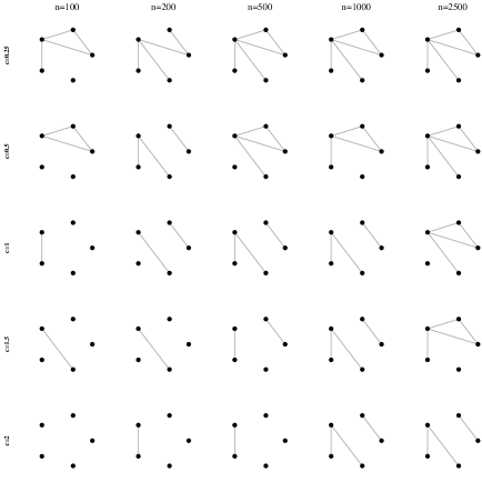
Figure 2: Estimated graph for neighbohood approach.

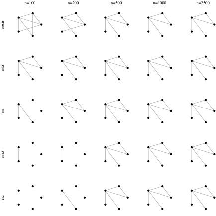
Figure 3: Estimated graph for neighbohood approach.

The algorithms implementing the graph estimators given by (13) (conservative approach) and (14) (non-conservative approach) were coded in the R language and are available as a package called mrfse in CRAN. In Figures 2 and 3 we show the results of both approaches, for values of the penalising constant $c$ in the set $\{0.25,0.5,1,1.5,2\}$ and sample sizes $n$ in the set $\{100,200,500,1000,2500\}$. In this example the non-conservative approach seems to converge to the underlying graph faster than the conservative approach. To evaluate this difference in a quantitative form, we compute a numeric value for the underestimation error (ue), overestimation error (oe) and total error (te), given by

$$ue\;=\;\dfrac{\sum_{(v,w)}\mathbf{1}\{(v,w)\in E\;\text{and}\;(v,w)\not\in\widehat{E})\}}{\sum_{(v,w)}\mathbf{1}\{(v,w)\in E\}}$$ (15)

$$oe\;=\;\dfrac{\sum_{(v,w)}\mathbf{1}\{(v,w)\not\in E\;\text{and}\;(v,w)\in\widehat{E})\}}{\sum_{(v,w)}\mathbf{1}\{(v,w)\notin E\}}\;$$ (16)

and

$$te\;=\;\dfrac{oe\sum_{(v,w)}\mathbf{1}\{(v,w)\in E\}+ue\sum_{(v,w)}\mathbf{1}\{(v,w)\not\in E\}}{|V|(|V|-1)}\,.$$ (17)

Figure 4 shows an evaluation of ue, oe and te for both methods, used with constant c = 1, and with sample sizes ranging from 100 to 10,000. The error lines corresponds to the mean errors in 30 runs of both algorithms.

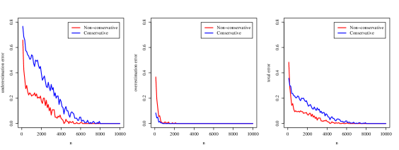
Figure 4: Mean of underestimation error (left), overestimation error (center) and total error (right) defined by (15)-(17), computed on 30 runs of the simulation, for both conservative and non-conservative approaches.

We also performed simulations for other distributions with different graph structures, specifically for the projected Markov chain in five variables given by Figure 1(a) (a graph with few edges) and the complete graph with five vertices (a graph with a maximum number of edges). We also simulated a distribution with 15 nodes, the same number of nodes considered in the application in Section 5. In all cases, the non-conservative approach seems to perform better than the conservative algorithm. The results are reported in the Supplementary material to this article.

5 Application on real data

To illustrate the performance of the estimator on real data we analyzed a stock index from fifteen countries on different times taken from the site https://br.investing.com/indices/world-indices. The countries are Brazil, USA, UK, France, India, Japan, Greece, Ireland, South Africa, Spain, Marroco, Australia, Mexico, China and Saudi Arabia with stock markets Bovespa, NASDAQ, FTSE 100, CAC 40, Nifty 50, Nikkei 225, FTSE ATHEX Large Cap, FTSE Ireland, FTSE South Africa, IBEX 35, Moroccan All Shares, S&P ASX 200, S&P BMV IPC, Shanghai Composite and Tadawul All Share, respectively. We collected 2120 entries where each entry contains the indicator function of an increasing variation in the stock index for a given day with respect to the previous day, for each one of the fifteen stock markets. That is, a stock market for a given day $d$ is codified as 1 if the stock index at day $d$ is greater than the stock index at day $d-1$, and 0 otherwise. The main goal is to estimate the conditional dependence graph between the codified stock markets corresponding to the fifteen countries. The dataset of stock index variation corresponds to subsequent time points (days) in the period from December $29^{th}$ of 2010 to October $22^{th}$ of 2018. To reduce sample correlation between subsequent observations we selected data points with a difference of 4 days. The final sample has a total of 530 time points. The datas are available in https://github.com/rodrigorsdc/ic/tree/master/stock_data

We applied the two approaches given by (13) and (14) to estimate the conditional dependence graph. We chose the penalising constant as $c=0.2$ by 10-Fold Cross-validation. The resulting graphs with the conservative and non-conservative approaches are shown in Figure 5. In both cases, the obtained graphs connect countries that are geographically near, as could be somehow expected. Also, the conservative approach underestimates a few edges compared to the non-conservative.

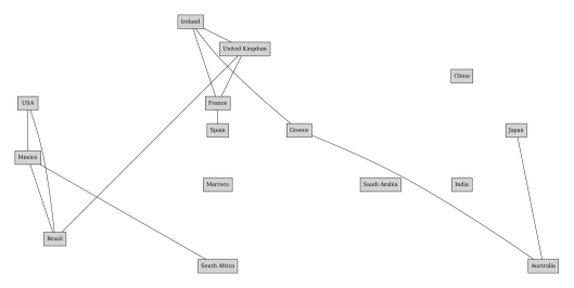
Figure 5: Estimated graphs with the conservative (top) and non-conservative (bottom) approaches. The constant $c$ in (3.2) used in both cases was $0.2$.

Discussion

In this paper we introduced an estimator for the basic neighborhood of a node in a general discrete Markov random field defined on a graph. We showed that the estimator is consistent for any value of the penalizing constant and is strongly consistent for a sufficiently large value of the constant. This result implies that any finite sub-graph can be recovered with probability one when the sample size diverges, provided the set of observed nodes increases not too fast or contains all the target nodes and its neighborhoods. The proof is based on some deviation inequalities given in Proposition 3.1, a result that is derived from a martingale approach appearing in [7] but that is new in this context of Markov random fields. One advantage of our results is that we do not need to assume a positivity condition, namely that all conditional probabilities in the model are strictly positive. This allows us to consider sparse models, that is models that can have many parameters equal to zero and then a low number of significant parameters, a property that is appealing on high dimensional contexts. We consider the samples of the Markov random field are independent and identically distributed, but one important question to address in future work is if this method can be generalised to dependent data, as for example the case of mixing processes as considered in [14].

Appendix: proof of theoretical results

Here we present the proofs of the main results in the paper, namely Lemma 2.3, Proposition 3.1, Theorem 3.3 and Corollary 3.4. We also prove some auxiliary results needed to demonstrate the main theorem in the article.

Proof of Lemma 2.3.

Suppose $w\notin\text{ne}(v)$. Take any $\Delta$ such that $\text{ne}(v)\subseteq\Delta,v\notin\Delta$. Then

$$p(a_{v}|a_{\Delta})=p(a_{v}|a_{\Delta\setminus\{w\}})\quad\mbox{ for all }a_{\Delta}\in A^{\Delta}\text{ with }p(a_{\Delta})>0.$$ (18)

By the definition of conditional probability and (18) we have that

$$p(a_{v},a_{w}|a_{\Delta\setminus\{w\}}) =p(a_{v}|a_{\Delta},a_{w})p(a_{w}|a_{\Delta\setminus\{w\}})$$ (19)

$$=p(a_{v}|a_{\Delta\setminus\{w\}})p(a_{w}|a_{\Delta\setminus\{w\}})$$

for all $a_{\Delta}$ with $p(a_{\Delta})>0$. But we also have that

$$p(a_{v},a_{w}|a_{\Delta\setminus\{w\}})=p(a_{w}|a_{\Delta\setminus\{w\}},a_{v})p(a_{v}|a_{\Delta\setminus\{w\}}).$$ (20)

Therefore, by (19) and (20), if $p(a_{v}|a_{\Delta\setminus\{w\}})>0$ we obtain

$$p(a_{w}|a_{\Delta\setminus\{w\}},a_{v})=p(a_{w}|a_{\Delta\setminus\{w\}})\,.$$

As the equality holds for all $\Delta$ and all $(a_{v},a_{\Delta\setminus\{w\}})$ with $p(a_{v},a_{\Delta\setminus\{w\}})>0$ then we conclude that $v\notin\text{ne}(w)$. ∎

Proof of Proposition 3.1.

First observe that

$$\begin{split}\mathbb{P}\Bigl{(}N(a_{W})\,\sup_{a_{v}\in A}&|\hat{p}(a_{v}|a_{W})-p(a_{v}|a_{W})|^{2}\;>\;\delta\log n\Bigr{)}\\ &\;\leq\;\sum_{a_{v}\in A}\mathbb{P}\Bigl{(}N(a_{W})\,|\hat{p}(a_{v}|a_{W})-p(a_{v}|a_{W})|^{2}\;>\;\delta\log n\Bigr{)}\end{split}$$ (21)

then we will fix $a_{v}\in A$ and bound above each term in the right hand side separately. For simplifying the notation we write $\hat{p}_{n}=\hat{p}(a_{v}|a_{W})$, $p=p(a_{v}|a_{W})$, $O_{n}=N(a_{v},a_{W})$ and $N_{n}=N(a_{W})$. Observe that $\hat{p}_{n}=O_{n}/N_{n}$. For $\lambda>0$ define $\phi(\lambda)=\log(1-p+2^{\lambda}p)$. Let $W^{\lambda}_{0}=1$ and for $n\geq 1$ define

$$W^{\lambda}_{n}=2^{\lambda O_{n}-N_{n}\phi(\lambda)}\,.$$

Observe that $W^{\lambda}_{n}$ is a martingale with respect to $\mathcal{F}_{n}=\sigma(X_{v,W}^{(1:n)},X_{W}^{(n+1)})$ and that $\mathbb{E}[\,W^{\lambda}_{n}\,]=1$. In fact, conditioned on $\mathcal{F}_{n}$ we have that

$$O_{n+1}-O_{n}=\begin{cases}1\,,&\text{if }x_{v}^{(n+1)}=a_{v},\,x_{W}^{(n+1)}=a_{W}\,;\\ 0\,,&\text{c.c }\,.\end{cases}$$

and similarly

$$N_{n+1}-N_{n}=\begin{cases}1\,,&\text{if }x_{W}^{(n+1)}=a_{W}\,;\\ 0\,,&\text{c.c }\,.\end{cases}$$

Observe that if $x_{W}^{(n+1)}=a_{W}$ then

$$\begin{split}\mathbb{E}\left[\,2^{\lambda(O_{n+1}-O_{n})}\,|\,\mathcal{F}_{n}\,\right]&=\mathbb{E}\left[\,2^{\lambda\mathbf{1}\{x_{v}^{(n+1)}=a_{v}\}}\,|\,\mathcal{F}_{n}\,\right]\\ &=2^{\phi(\lambda)}\\ &=2^{(N_{n+1}-N_{n})\phi(\lambda)}\,.\end{split}$$ (22)

On the other hand, if $x_{W}^{(n+1)}\neq a_{W}$ the equality trivially holds. Then rearranging the terms in (22) we conclude that

$$\mathbb{E}\left[2^{\lambda O_{n+1}-N_{n+1}\phi(\lambda)}\,|\,\mathcal{F}_{n}\right]=2^{\lambda O_{n}-N_{n}\phi(\lambda)}$$

and $W^{\lambda}_{n}$ is a martingale with respect to $\mathcal{F}_{n}$. Now divide the interval $\{1,\dots,n\}$ of possible values of $N_{n}$ into “slices” $\{t_{k-1}+1,\dots,t_{k}\}$ of geometrically increasing size, and treat the slices independently. We take $\alpha=\delta\log n$ and we assume that $n$ is sufficiently large so that $\alpha>1$. Take $\eta=1/(\alpha-1)$, $t_{0}=0$ and for $k\geq 1$, $t_{k}=\left\lfloor(1+\eta)^{k}\right\rfloor$. Let $m$ be the first integer such that $t_{m}\geq n$, that is

$$m=\left\lceil\frac{\log n}{\log(1+\eta)}\right\rceil\,.$$

Define the events $B_{k}=\left\{t_{k-1}<N_{n}\leq t_{k}\right\}\cap\bigl{\{}N_{n}\,|\hat{p}_{n}-p|^{2}>\alpha\bigr{\}}$. We have

$$\mathbb{P}\left(N_{n}\,|\hat{p}_{n}-p|^{2}\;>\;\alpha\right)\;\leq\;\mathbb{P}\biggl{(}\bigcup_{k=1}^{m}B_{k}\biggr{)}\;\leq\;\sum_{k=1}^{m}\mathbb{P}\left(B_{k}\right).$$ (23)

Without loss of generality we can assume that $\hat{p}\geq p$ (the case $\hat{p}\leq p$ holds by symmetry). Observe that $|x-p|^{2}$ is a continuous increasing function for $x\in[p;1]$, with $0\leq|x-p|^{2}\leq|1-p|^{2}$. Let $x$ be such that $|x-p|^{2}=\alpha/(1+\eta)^{k}$, that is we take

$$x\;=\;\sqrt{\frac{\alpha}{(1+\eta)^{k}}}+p\,.$$

Observe that $x\in[p,1]$ unless $\alpha/(1+\eta)^{k}>|1-p|^{2}$. But in this case we have that if $N_{n}\leq(1+\eta)^{k}$ then

$$\alpha\;>\;(1+\eta)^{k}|1-p|^{2}\;\geq\;N_{n}|\hat{p}_{n}-p|^{2}$$

so $\mathbb{P}(B_{k})=0$. So we may assume that such an $x$ always exists over the non-empty events $B_{k}$. Moreover, on $B_{k}$ we have that $|\hat{p}_{n}-p|^{2}\geq\alpha/N_{n}\geq\alpha/(1+\eta)^{k}$ then we must have $\hat{p}_{n}\geq x$. Now take $\lambda=\log(x(1-p))-\log(p(1-x))$. It can be verified that $\lambda x-\phi(\lambda)=d(x;p)\geq|x-p|^{2}$. Then on $B_{k}$ we have that

$$\lambda\hat{p}_{n}-\phi(\lambda)\;\geq\;\lambda x-\phi(\lambda)\;\geq\;|x-p|^{2}\;=\;\frac{\alpha}{(1+\eta)^{k}}\;\geq\;\frac{\alpha}{(1+\eta)N_{n}}$$

therefore

$$B_{k} \;\subset\;\left\{\lambda\hat{p}_{n}-\phi(\lambda)\,>\,\frac{\alpha}{(1+\eta)N_{n}}\right\}$$

$$\;\subset\;\left\{W_{n}^{\lambda}\,>\,2^{\alpha/(1+\eta)}\right\}.$$

As $\mathbb{E}\bigl{[}W_{n}^{\lambda}\bigr{]}=1$, Markov’s inequality implies that

$$\mathbb{P}\left(B_{k}\right) \;\leq\;\mathbb{P}\left(W_{n}^{\lambda}>2^{\alpha/(1+\eta)}\right)$$ (24)

$$\;\leq\;2^{-\alpha/(1+\eta)}.$$

Finally, by (23) we have that

$$\mathbb{P}\left(N_{n}|\hat{p}_{n}-p|^{2}\;>\;\alpha\right)\;\leq\;m\,2^{-\alpha/(1+\eta)}.$$

But as $\eta=1/(\alpha-1)$, $m=\left\lceil\frac{\log n}{\log(1+\eta)}\right\rceil$ and $\log(1+1/(\alpha-1))\geq 1/\alpha$ we obtain

$$\mathbb{P}\left(N_{n}\,|\hat{p}_{n}-p|^{2}\;>\;\alpha\right)\;\leq\;2\alpha\log(n)2^{-\alpha}\;=\;\frac{2\delta\log^{2}(n)}{n^{\delta}}.$$

Finally, by (21) we obtain that

$$\mathbb{P}\Bigl{(}N(a_{W})\,\sup_{a_{v}\in A}|\hat{p}(a_{v}|a_{W})-p(a_{v}|a_{W})|^{2}\;>\;\delta\log n\Bigr{)}\;\leq\;\frac{2|A|\delta\log^{2}n}{n^{\delta}}\,.\qed$$

Now we state a result controlling the probability in Proposition 3.1 for all possible neighbourhoods at the same time.

Proposition 5.1.

For all $\delta>0$, all $v\in V_{n}$ and $|V_{n}|=o(\log n)$ we have

$$\mathbb{P}\Bigl{(}\,\sup_{W\subset V_{n}\setminus\{v\}}\sup_{a_{W}\in A^{W}}\sup_{a_{v}\in A}\;N(a_{W})\,|\hat{p}(a_{v}|a_{W})-p(a_{v}|a_{W})|^{2}\;<\,\delta\log n\,\Bigr{)}\;\rightarrow\;1$$

when $n\to\infty$. Moreover, if $\delta>1$ then the probability equals one for all sufficiently large $n$.

Proof.

Assume $|V_{n}|=\epsilon_{n}\log n$, with $\epsilon_{n}\to 0$ when $n\to\infty$. By Proposition 3.1 and a union bound we have that

$$\begin{split}\mathbb{P}\Bigl{(}\sup_{W\subset V_{n}\setminus\{v\}}\sup_{a_{W}\in A^{W}}\sup_{a_{v}\in A}\;N(a_{W})\,|\hat{p}(a_{v}|a_{W})-&p(a_{v}|a_{W})|^{2}\;>\;\delta\log n\Bigr{)}\\ &\;\leq\;\,2^{|V_{n}|}|A|^{|V_{n}|}\frac{2|A|\delta\log^{2}n}{n^{\delta}}\\ &\;\leq\;\,\frac{c\delta\log^{2}n}{n^{\delta-2\epsilon_{n}}}\,.\end{split}$$

For $\delta>0$ the bound on the right-hand side converges to 0 and it is summable in $n$ for any $\delta>1$. Then the almost sure convergence follows by the Borel-Cantelli lemma. ∎

The following basic result about the Küllback-Leibler divergence corresponds to [3, Lemma 6.3]. We omit its proof here.

Lemma 5.2.

For any $P$ and $Q$ we have

$$D(P;Q)\;\leq\;\sum_{a\in A\colon Q(a)>0}\frac{[P(a)-Q(a)]^{2}}{Q(a)}\,.$$

The next lemma was proved in [3, Lemma A.2] for translation invariant Markov random fields. As our setting is different, we include its proof here.

Lemma 5.3.

If a neighborhood $W$ of $v\in V$ satisfies

$$p(a_{v}|a_{W})=p(a_{v}|a_{\text{ne}(v)})$$

for all $a_{v}\in A$, and all $a_{W\cup\text{ne}(v)}\in A^{W\cup\text{ne}(v)}$ with $p(a_{W\cup\text{ne}(v)})>0$ then $W$ is a Markov neighborhood.

Proof.

We have to show that for any $\Delta\subset V$ finite, with $\Delta\supset W$,

$$p(a_{v}|a_{\Delta})=p(a_{v}|a_{W})$$ (25)

for all $a_{v}\in A$ and all $a_{\Delta}\in A^{\Delta}$ with $p(a_{\Delta})>0$. As $\text{ne}(v)$ is a Markov neighborhood, the lemma’s condition implies

$$p(a_{v}|a_{W})=p(a_{v}|a_{\text{ne}(v)})=p(a_{v}|a_{\text{ne}(v)\cup\Delta})$$

or all $a_{v}\in A$ and all $a_{\text{ne}(v)\cup\Delta}\in A^{\text{ne}(v)\cup\Delta}$ with $p(a_{\text{ne}(v)\cup\Delta})>0$. So (25) follows, because $W\subseteq\Delta\subseteq\text{ne}(v)\cup\Delta$. ∎

The following proposition guarantees uniform control of all empirical marginal probabilities for subsets of variables in $V_{n}$.

Proposition 5.4.

Let $\{V_{n}\}_{n\in\mathbb{N}}$ be such that $|V_{n}|=o(\log n)$. Then for all $\delta>2$ we have

$$|\hat{p}(a_{W})-p(a_{W})|\;<\;\sqrt{\frac{\delta\log n}{n}}$$

simultaneously for all $W\subseteq V_{n}$ and $a_{W}\in A^{W}$, eventually almost surely as $n\rightarrow\infty$.

Proof.

For $W\subset V_{n}$ and $a_{W}\in A^{W}$ define

$$Y_{i}(a_{W})=\mathbf{1}\{x_{W}^{(i)}=a_{W}\}-p(a_{W})\,,\quad\;i=1,2,\ldots,n.$$

Note that $\mathbb{E}(Y_{i}(a_{W}))=0$ and $|Y_{i}(a_{W})|\leq 1$ for all $i=1,2,\ldots,n$. Then by Hoeffding’s Inequality we have that

$$\mathbb{P}\Bigl{(}\,\Bigl{|}\frac{1}{n}\sum_{i=1}^{n}Y_{i}(a_{W})- \mathbb{E}\Bigl{[}\frac{1}{n}\sum_{i=1}^{n}Y_{i}(a_{W})\Bigr{]}\Bigr{|}\geq t\Bigr{)}\;\leq\;2\exp\bigl{(}-\frac{nt^{2}}{2}\bigr{)}\,.$$

Observe that

$$\frac{1}{n}\sum_{i=1}^{n}Y_{i}(a_{W})=\frac{N(a_{W})}{n}-p(a_{W})$$

and

$$\mathbb{E}\Bigl{[}\frac{1}{n}\sum_{i=1}^{n}Y_{i}(a_{W})\Bigr{]}=0\,.$$

Therefore

$$\mathbb{P}\Bigl{(}\Bigl{|}\frac{N(a_{W})}{n}-p(a_{W})\Bigr{|}\geq t\Bigr{)}\;\leq\;2\exp\bigl{(}-\frac{nt^{2}}{2}\bigr{)}\,.$$

Taking $t=\sqrt{\frac{\delta\log n}{n}}$ we have that

$$\mathbb{P}\Bigl{(}\bigl{|}\hat{p}(a_{W})- p(a_{W})\bigl{|}\geq\sqrt{\frac{\delta\log n}{n}}\mbox{ for some }W\subset V_{n}\mbox{ and }a_{W}\in A^{W}\Bigr{)}$$

$$\leq\;\sum_{W\subset V_{n}}\sum_{a_{W}\in A^{W}}\mathbb{P}\Bigl{(}\bigl{|}\hat{p}(a_{W})-p(a_{W})\bigr{|}\geq\sqrt{\frac{\delta\log n}{n}}\Bigr{)}$$

$$\leq\;2^{|V_{n}|}|A|^{|V_{n}|}\,2\exp\bigl{(}-\frac{\delta\log n}{2}\bigr{)}$$

which is summable in $n$ for $\delta>2$. This completes the proof. ∎

Proof of Theorem 3.3.

Denote by

$$\text{\sc{PML}}(x_{v}^{(1:n)}|x_{W}^{(1:n)})\;=\;\log\hat{\mathbb{P}}(x_{v}^{(1:n)}|x_{W}^{(1:n)})-c|A|^{|W|}\log n\,,$$

where $\hat{\mathbb{P}}(x_{v}^{(1:n)}|x_{W}^{(1:n)})$ is given by (10). If $V_{n}\setminus\{v\}$ is the bounding set for the candidate neighborhoods of vertex $v$ and $\text{ne}(v)$ is the basic neighborhood of $v$, we need to prove that for any $c>0$

$$\max_{W\subset V_{n}\setminus\{v\},W\neq\text{ne}(v)}\text{\sc{PML}}(x_{v}^{(1:n)}|x_{W}^{(1:n)})\;<\;\text{\sc{PML}}(x_{v}^{(1:n)}|x_{\text{ne}(v)}^{(1:n)})$$ (26)

with probability converging to 1 when $n\to\infty$. Moreover, for $c>[p_{\min}(v)(|A|-1)]^{-1}$ we need to prove that (26) holds eventually almost surely as $n\to\infty$. We divide the proof in two cases, showing that

$$\max_{W\in\mathcal{B}_{i}}\text{\sc{PML}}(x_{v}^{(1:n)}|x_{W}^{(1:n)})\;<\;\text{\sc{PML}}(x_{v}^{(1:n)}|x_{\text{ne}(v)}^{(1:n)})$$ (27)

with high probability or almost surely as $n\to\infty$, depending on the value of $c$, for $i=1,2$ where

• $\mathcal{B}_{1}=\{W\subset V_{n}\setminus\{v\}\colon\text{ne}(v)\subsetneq W\}$

• $\mathcal{B}_{2}=\{W\subset V_{n}\setminus\{v\}\colon\text{ne}(v)\not\subset W\}$

For case (a), observe that for all $W\in\mathcal{B}_{1}$

$$\text{\sc{PML}}(x_{v}^{(1:n)} |x_{\text{ne}(v)}^{(1:n)})-\text{\sc{PML}}(x_{v}^{(1:n)}|x_{W}^{(1:n)})\;=$$ (28)

$$\qquad c\,(|A|^{|W|}-|A|^{|\text{ne}(v)|})\log n\;-\sum_{a_{v},a_{W}\in A^{|W|+1}}N(a_{v},a_{W})\log\frac{\hat{p}(a_{v}|a_{W})}{\hat{p}(a_{v}|a_{\text{ne}(v)})}\,.$$

As these empirical probabilities are the maximum likelihood estimators of the conditional probabilities and $\text{ne}(v)\subset W$ we have that

$$\sum_{a_{v},a_{W}\in A^{W+1}}N(a_{v},a_{W})\log\hat{p}(a_{v}|a_{\text{ne}(v)})\; \geq\;\sum_{a_{v},a_{W}\in A^{W+1}}N(a_{v},a_{W})\log p(a_{v}|a_{\text{ne}(v)})$$

$$=\;\sum_{a_{v},a_{W}\in A^{W+1}}N(a_{v},a_{W})\log p(a_{v}|a_{W})\,.$$

Therefore, (28) can be lower-bounded by

$$c\,\left(1-\frac{1}{|A|}\right)|A|^{|W|}\log n\;-\sum_{a_{v},a_{W}\in A^{W+1}}N(a_{v},a_{W})\log\frac{\hat{p}(a_{v}|a_{W})}{p(a_{v}|a_{W})}\,.$$ (29)

Note that

$$\sum_{a_{v},a_{W}\in A^{W+1}}N(a_{v},a_{W})\log\frac{\hat{p}(a_{v}|a_{W})}{p(a_{v}|a_{W})}=\sum_{a_{W}\in A^{W}}N(a_{W})D(\hat{p}(\cdot_{v}|a_{W})\,;\,p(\cdot_{v}|a_{W}))\,,$$

where $D$ denotes the Küllback-Leibler divergence, see (12). Therefore we have, by Lemma 5.2, that

$$\begin{split}\sum_{a_{W}\in A^{W}}N(a_{W})&D(\hat{p}(\cdot_{v}|a_{W})\,;\,p(\cdot_{v}|a_{W}))\\ &\leq\;\sum_{a_{W}\in A^{W}}N(a_{W})\sum_{a_{v}\in A}\frac{[\,\hat{p}(a_{v}|a_{W})-p(a_{v}|a_{W})\,]^{2}}{p(a_{v}|a_{W})}.\end{split}$$ (30)

Then, by Proposition 5.1 with $\delta>0$ and (30) we have, with probability converging to 1 that

$$\sup_{W\in\mathcal{B}_{1}}\sum_{a_{W}\in A^{W}}N(a_{W}) D(\hat{p}(\cdot_{v}|a_{W})\,;\,p(\cdot_{v}|a_{W}))$$

$$\leq\;\frac{\delta|A|^{|W|+1}\log n}{p_{*}}$$

and this holds eventually almost surely if $\delta>1$. Then the difference (29) can be lower bounded by

$$c\,\left(1-\frac{1}{|A|}\right)|A|^{|W|}\log n-\frac{\delta|A|^{|W|+1}\log n}{p_{*}}\;>\;0$$

if $\delta<c(|A|-1)|A|^{-2}p_{*}$. Then, for any $c>0$ there exists a sufficiently small $\delta>0$ such that

$$\max_{W\in\mathcal{B}_{1}}\text{\sc{PML}}(x_{v}^{(1:n)}|x_{W}^{(1:n)})\;<\;\text{\sc{PML}}(x_{v}^{(1:n)}|x_{\text{ne}(v)}^{(1:n)})$$

with probability converging to one. Moreover, if $c>|A|^{2}[p_{*}(|A|-1)]^{-1}$ we can take $\delta>1$ in Proposition 5.1 and we have that this inequality holds eventually almost surely as $n\to\infty$. This completes the proof of (27) for case (a).
Finally, to prove (27) in case (b) we will first prove that

$$\max_{W\in\mathcal{B}_{2}}\text{\sc{PML}}(x_{v}^{(1:n)}|x_{W}^{(1:n)})\;\leq\;\text{\sc{PML}}(x_{v}^{(1:n)}|x_{V_{n}\setminus\{v\}}^{(1:n)})$$

eventually almost surely as $n\to\infty$. This inequality together with case (a) will imply (27) for $i=2$. Note that we have

$$\text{\sc{PML}}(x_{v}^{(1:n)} |x_{V_{n}\setminus\{v\}}^{(1:n)})-\text{\sc{PML}}(x_{v}^{(1:n)}|x_{W}^{(1:n)})$$

$$=\; \sum_{a_{V_{n}}\in A^{V_{n}}}N(a_{v},a_{V_{n}\setminus\{v\}})\log\frac{\hat{p}(a_{v}|a_{V_{n}\setminus\{v\}})}{\hat{p}(a_{v}|a_{W})}-c\,(|A|^{|V_{n}|-1}-|A|^{|W|})\log n$$

$$=\; \;n\Biggl{[}\;\sum_{a_{V_{n}}\in A^{V_{n}}}\frac{N(a_{V_{n}})}{n}\log\frac{\hat{p}(a_{v}|a_{V_{n}\setminus\{v\}})}{\hat{p}(a_{v}|a_{W})}-c\,(|A|^{|V_{n}|-1}-|A|^{|W|})\frac{\log n}{n}\Biggr{]}\,.$$

Observe that for the second term into de brackets we have

$$c\,(|A|^{|V_{n}|-1}-|A|^{|W|})\frac{\log n}{n}\;\longrightarrow\;0$$

when $n\to\infty$, because we are assuming $|V_{n}|=o(\log n)$. For the first term by summing and subtracting $\frac{N(a_{V_{n}})}{n}\log p(a_{v}|a_{W})$ inside the sum we have that

$$\sum_{a_{V_{n}}}\;\,\frac{N(a_{V_{n}})}{n} \log\frac{\hat{p}(a_{v}|a_{V_{n}\setminus\{v\}})}{\hat{p}(a_{v}|a_{W})}$$

$$= \;\sum_{a_{V_{n}}}\left[\frac{N(a_{V_{n}})}{n}\log\frac{\hat{p}(a_{v}|a_{V_{n}\setminus\{v\}})}{p(a_{v}|a_{W})}-\frac{N(a_{V_{n}})}{n}\log\frac{\hat{p}(a_{v}|a_{W})}{p(a_{v}|a_{W})}\right].$$ (31)

We divide again the expression in two parts. By one hand, by looking at the second term of the sum in (Proof of Theorem 3.3.) we have that

$$\sum_{a_{V_{n}}}\frac{N(a_{V_{n}})}{n}\log\frac{\hat{p}(a_{v}|a_{W})}{p(a_{v}|a_{W})} =\sum_{(a_{v},a_{W})\in A^{1+W}}\frac{N(a_{v},a_{W})}{n}\log\frac{\hat{p}(a_{v}|a_{W})}{p(a_{v}|a_{W})}$$

$$=\sum_{(a_{v},a_{W})\in A^{1+W}}\frac{N(a_{W})}{n}\hat{p}(a_{v}|a_{W})\log\frac{\hat{p}(a_{v}|a_{W})}{p(a_{v}|a_{W})}$$

$$=\sum_{a_{W}\in A^{W}}\frac{N(a_{W})}{n}D(\hat{p}(\cdot_{v}|a_{W})\,;\,p(\cdot_{v}|a_{W})).$$

By Lemma 5.2 and Proposition 5.1 we have that

$$\begin{split}\max_{W\in\mathcal{B}_{2}}\;\sum_{a_{W}\in A^{W}}\frac{N(a_{W})}{n}D(\hat{p}(\cdot_{v}|a_{W})\,;\,p(\cdot_{v}|a_{W}))\;&\leq\;\sum_{a_{W}\in A^{W}}\frac{N(a_{W})}{n}\sum_{a_{v}\in A}\frac{[\,\hat{p}(a_{v}|a_{W})-p(a_{v}|a_{W})\,]^{2}}{p(a_{v}|a_{W})}\\ &\leq\;\,\max_{W\in\mathcal{B}_{2}}\frac{|A|^{|W|+1}\delta\log n}{p_{*}\,n}\;\longrightarrow\;0\end{split}$$ (32)

eventually almost surely as $n\to\infty$, for $\delta>1$. On the other hand, as $\hat{p}(a_{v}|a_{V_{n}\setminus\{v\}})$ are the maximum likelihood estimators of $p(a_{v}|a_{V_{n}\setminus\{v\}})$ and as $V_{n}$ will eventually contain $\text{ne}(v)$, the first term in the sum (Proof of Theorem 3.3.) can be lower-bounded by

$$\begin{split}\sum_{a_{V_{n}}}\frac{N(a_{V_{n}})}{n}\log\frac{p(a_{v}|a_{V_{n}\setminus\{v\}})}{p(a_{v}|a_{W})}&\;=\;\sum_{a_{v}}\sum_{a_{W\cup\text{ne}(v)}}\frac{N(a_{v},a_{W\cup\text{ne}(v)})}{n}\log\frac{p(a_{v}|a_{\text{ne}(v)})}{p(a_{v}|a_{W})}\,.\end{split}$$ (33)

By Proposition 5.4 we have that

$$\frac{N(a_{v},a_{W\cup\text{ne}(v)})}{n}\;\geq\;p(a_{v},a_{W\cup\text{ne}(v)})-\sqrt{\frac{3\log n}{n}}$$

eventually almost surely, simultaneously for all $W$ and all $(a_{v},a_{W\cup\text{ne}(v)}))$. Then, (33) can be lower bounded by

$$\begin{split}\sum_{a_{W\cup\text{ne}(v)}}p(a_{W\cup\text{ne}(v)})D(p(\cdot_{v}|a_{\text{ne}(v)})\,;\,p(\cdot_{v}|a_{W}))-\sqrt{\frac{3\log n}{n}}\sum_{a_{W\cup\text{ne}(v)}}\log\frac{p(a_{v}|a_{\text{ne}(v)})}{p(a_{v}|a_{W})}&\;\geq\;\frac{\alpha_{*}}{2}\end{split}$$ (34)

eventually almost surely as $n\to\infty$. Therefore

$$\max_{W\in\mathcal{B}_{2}}\;\text{\sc{PML}}(x_{v}^{(1:n)}|x_{W}^{(1:n)})\;\leq\;\text{\sc{PML}}(x_{v}^{(1:n)}|x_{V_{n}\setminus\{v\}}^{(1:n)})$$

eventually almost surely as $n\to\infty$. As $V_{n}$ will contain $\text{ne}(v)$ for $n$ sufficiently large, then $V_{n}\setminus\{v\}\in\mathcal{B}_{1}$ for such values of $n$. Then, by case (a) we have

$$\text{\sc{PML}}(x_{v}^{(1:n)}|x_{V_{n}\setminus\{v\}}^{(1:n)})\;\leq\;\max_{W\in\mathcal{B}_{1}}\text{\sc{PML}}(x_{v}^{(1:n)}|x_{W}^{(1:n)})\;<\;\text{\sc{PML}}(x_{v}^{(1:n)}|x_{\text{ne}(v)}^{(1:n)})$$

eventually almost surely as $n\to\infty$, and this finishes the proof of case (b). By combining the results of the two cases, we conclude that

$$\max_{W\subset V_{n}\setminus\{v\},W\neq\text{ne}(v)}\text{\sc{PML}}(x_{v}^{(1:n)}|x_{W}^{(1:n)})\;<\;\text{\sc{PML}}(x_{v}^{(1:n)}|x_{\text{ne}(v)}^{(1:n)})$$

and that $\widehat{\text{ne}}(v)=\text{ne}(v)$, with probability converging to 1 for all $c>0$, or eventually almost surely as $n\to\infty$, for $c>|A|^{2}[p_{*}(|A|-1)]^{-1}$. ∎

Proof of Corollary 3.4.

The proof of the corollary follows from Theorem 3.3 and the fact that $V^{\prime}$ is finite. ∎

References

- [1] Yves F. Atchade. Estimation of high-dimensional partially-observed discrete markov random fields. Electron. J. Statist., 8(2):2242–2263, 2014.
- [2] Guy Bresler, David Gamarnik, and Devavrat Shah. Learning graphical models from the Glauber dynamics. IEEE Trans. Inform. Theory, 64(6):4072–4080, 2018.
- [3] Imre Csiszár and Zsolt Talata. Consistent estimation of the basic neighborhood of Markov random fields. Ann. Statist., 34(1):123–145, 2006.
- [4] Fabio Divino, Arnoldo Frigessi, and Peter J. Green. Penalized pseudolikelihood inference in spatial interaction models with covariates. Scandinavian Journal of Statistics, 27(3):445–458, 2000.
- [5] Aline Duarte, Antonio Galves, Eva Löcherbach, and Guilherme Ost. Estimating the interaction graph of stochastic neural dynamics. Bernoulli, 25(1):771–792, 2019.
- [6] Antonio Galves, Enza Orlandi, and Daniel Y. Takahashi. Identifying interacting pairs of sites in Ising models on a countable set. Braz. J. Probab. Stat., 29(2):443–459, 2015.
- [7] A. Garivier and F. Leonardi. Context tree selection: A unifying view. Stochastic Processes and their Applications, 121(11):2488 – 2506, 2011.
- [8] Hans-Otto Georgii. Gibbs measures and phase transitions, volume 9 of de Gruyter Studies in Mathematics. Walter de Gruyter & Co., Berlin, second edition, 2011.
- [9] J. M. Hammersley and P. Clifford. Markov fields on finite graphs and lattices. Unpublished manuscript. Available at http://www.statslab.cam.ac.uk/~grg/books/hammfest/hamm-cliff.pdf, 1971.
- [10] Holger Höfling and Robert Tibshirani. Estimation of sparse binary pairwise markov networks using pseudo-likelihoods. Journal of Machine Learning Research, 10(32):883–906, 2009.
- [11] Daphne Koller and Nir Friedman. Probabilistic Graphical Models: Principles and Techniques - Adaptive Computation and Machine Learning. The MIT Press, 2009.
- [12] John Lafferty, Han Liu, and Larry Wasserman. Sparse Nonparametric Graphical Models. Statistical Science, 27(4):519 – 537, 2012.
- [13] Steffen L. Lauritzen. Graphical Models. Oxford University Press, 1996.
- [14] Florencia Leonardi, Matías Lopez-Rosenfeldz, Daniela Rodriguez, Magno T. F. Severino, and Mariela Sued. Independent block identification in multivariate time series. Journal of Time Series Analysis (accepted), 42(1):19–33, 2020.
- [15] Matthieu Lerasle and Daniel Y. Takahashi. Sharp oracle inequalities and slope heuristic for specification probabilities estimation in discrete random fields. Bernoulli, 22(1):325–344, 2016.
- [16] Han Liu, Fang Han, Ming Yuan, John Lafferty, and Larry Wasserman. High-dimensional semiparametric Gaussian copula graphical models. The Annals of Statistics, 40(4):2293 – 2326, 2012.
- [17] Eva Löcherbach and Enza Orlandi. Neighborhood radius estimation for variable-neighborhood random fields. Stochastic Process. Appl., 121(9):2151–2185, 2011.
- [18] Po-Ling Loh and Martin J. Wainwright. Structure estimation for discrete graphical models: Generalized covariance matrices and their inverses. Ann. Statist., 41(6):3022–3049, 2013.
- [19] N. Meinshausen and P. Bühlmann. High-dimensional graphs and variable selection with the lasso. Ann. Statist., 34(3):1436–1462, 2006.
- [20] Johan Pensar, Henrik Nyman, and Jukka Corander. Structure learning of contextual markov networks using marginal pseudo-likelihood. Scandinavian Journal of Statistics, 44(2):455–479, 2017.
- [21] Pradeep Ravikumar, Martin J. Wainwright, and John D. Lafferty. High-dimensional Ising model selection using -regularized logistic regression. Ann. Statist., 38(3):3022–1319, 2010.
- [22] Narayana P. Santhanam and Martin J. Wainwright. Information-theoretic limits of selecting binary graphical models in high dimensions. IEEE Trans. Inform. Theory, 58(7):4117–4134, 2012.
- [23] G. Schwarz. Estimating the dimension of a model. Ann. Statist., 6:461–464, 1978.
- [24] A. Shojaie and G. Michailidis. Penalized likelihood methods for estimation of sparse high-dimensional directed acyclic graphs. Biometrika, 97(3):519–538, 2010.
- [25] David Strauss and Michael Ikeda. Pseudolikelihood Estimation for Social Networks. Journal of the American Statistical Association,, 85(409):204–212, 1990.
- [26] Håkon Tjelmeland and Julian Besag. Markov random fields with higher-order interactions. Scandinavian Journal of Statistics, 25(3):415–433, 1998.
- [27] Eunho Yang, Pradeep Ravikumar, Genevera I. Allen, and Zhandong Liu. Graphical models via univariate exponential family distributions. Journal of Machine Learning Research, 16(115):3813–3847, 2015.