An Algebraic Geometric Foundation for a Classification of Superintegrable Systems in Arbitrary Dimension

Abstract.

Second-order superintegrable systems in dimensions two and three are essentially classified. With increasing dimension, however, the non-linear partial differential equations employed in current methods become unmanageable. Here we propose a new, algebraic-geometric approach to the classification problem – based on a proof that the classification space for irreducible non-degenerate second-order superintegrable systems is naturally endowed with the structure of a quasi-projective variety with a linear isometry action. On constant curvature manifolds our approach leads to a single, simple and explicit algebraic equation defining the variety classifying superintegrable Hamiltonians that satisfy all relevant integrability conditions generically. In particular, this includes all non-degenerate superintegrable systems known to date and shows that our approach is manageable in arbitrary dimension. Our work establishes the foundations for a complete classification of second-order superintegrable systems in arbitrary dimension, derived from the geometry of the classification space, with many potential applications to related structures such as quadratic symmetry algebras and special functions.

1. Introduction

It is a puzzling happenstance that the fundamental equations of nature admit explicit analytic solutions, at least for simple models. Think of Schrödinger’s Equation for the hydrogen atom, for instance: Its explicit solutions describe the shape of the atomic orbits and explain many of the physical and chemical properties of over hundred elements known today. The existence of explicit solutions in this case stems from a deeper fact – the hydrogen atom is a superintegrable system. The present paper develops methods to explore such systems systematically and exhaustively in arbitrary dimension.

1.1. What are superintegrable systems?

Symmetries are an essential tool in the study of Hamiltonian systems, and superintegrable systems are the most symmetric of these. The prototypical example of a superintegrable system is the Kepler system of planetary motion around a central celestial body. By the nature of the equations of motion, the movement of the planet is completely determined by its position and momentum given at any fixed point in time. More abstractly, the movement defines a curve in the six-dimensional phase-space of position and momentum.

In a conservative central force field, the energy and the angular momentum vector are conserved under the temporal evolution of the system. The Kepler system has the remarkable property that it possesses an additional conserved quantity: the Laplace-Runge-Lenz vector, pointing from the force centre towards the perihelion of the planetary orbit. Together, these form seven scalar constants of motion. Each of them defines a function on phase-space and confines the trajectory of the system to a level set of this function. Since phase space is six-dimensional, only five out of them can be functionally independent. Indeed, there are two scalar identities among them.

The quantum counterpart of the Kepler system is the aforementioned model of the hydrogen atom. Its conserved quantities are represented by quantum numbers, which constitute the ordering principle behind the Periodic Table of Elements.

With the Kepler system in mind, a (maximally) superintegrable system is defined as a Hamiltonian system of arbitrary dimension $n$ possessing the maximal number of functionally independent constants of motion, which is $2n-1$. The superintegrable system is called quadratic if the constants of motion can be chosen quadratic in the momenta.

The study of superintegrable systems has a long standing history due to the attractive possibility of determining almost all important features using algebraic methods alone. Beyond this obvious motivation, worthwhile in its own right, there exists also a deeper aspiration to classify superintegrable systems: They give rise to a large class of special functions.

1.2. Special functions and superintegrable systems

Since the appearance of the first tables of chords [Ptory], special functions have been ubiquitous in science and technology. Their fundamental role necessitates not only explicit formulae or the tabulation of a function’s values, but also a thorough documentation of its properties and interrelations. Traditionally, this has been done in the form of handbooks, most notably the Bateman Manuscript Project [Bat53, Bat54], filling five thick volumes, and the “Abramowitz and Stegun” Handbook of Mathematical Functions [AS], with more than 40,000 citations one of the most cited works in the literature [BCLO11]. In the dawn of the era of digitisation, the use of sophisticated symbolic computation engines has overcome the limitations of books and manual calculations, and handbooks have been replaced by extensive online databases. The most complete resources today are the Mathematical Functions Site [WMT], which comprises at present more than 300,000 formulae and is steadily growing, and the NIST Digital Library of Mathematical Functions [DLMF], the online version of the above mentioned Handbook of Mathematical Functions.

Yet, special functions have always been organised in an ad hoc manner and all handbooks and databases are mere compilations. Meanwhile, the search for a unified theory of special functions has continued since the nineteenth century – a theory that would explain and systematically organise, for a reasonably wide class of special functions, their properties, interrelations, symmetry principles and other related structures behind the façade of seemingly endless formulae in rows.

A theory aiming to classify special functions may naturally start from some rich source of such functions. This is where superintegrable systems come into play: Besides the hypergeometric differential equation, they are a particularly prolific source of special functions. Notably, it has been shown that superintegrable systems give rise to hypergeometric orthogonal polynomials [KMP07, KMP13], to Painlevé transcendants [MPR20, Gra04], to Jacobi-Dunkl polynomials [GIVZ13], and to the recently discovered exceptional polynomials [PTV12, HMPZ18].

The present work establishes the foundations for a complete classification of second-order superintegrable systems and thereby lays the foundation for subsequent research leading to such a theory – a “Periodic Table of Special Functions”, so to speak, comprising a wide variety of special functions derived from a sequence of projective $G$-varieties whose dimensions and geometric invariants play the role of the atomic and quantum numbers in the Periodic Table of Elements. In analogy to the Schrödinger Equation, which provides the basis for a systematic mathematical description of chemical elements and their properties, we establish a single, simple equation defining these varieties, which provides the basis for a systematic algebraic-geometric description of special functions and their properties.

1.3. Classification of superintegable systems – State-of-the-art

To date, the most well-developed results on the classification and structure concern second-order (conformally) superintegrable systems on conformally flat spaces in dimensions two and three. In particular, such results exist for the Euclidean plane [Tem04, KKM07b], Darboux-Koenigs spaces [KKW02, KKMW03], general 2D spaces [DY06, KKM05a, KKM05b], degenerate 2D superintegrable systems [KKMP09], quantum 2D superintegrable systems [BDK93, KKM06b, DT07], 3D flat space [KKM07c], 3D conformally flat spaces [KKM05c, KKM06a, KKM07a, KKM07c, CK14] and for quantum superintegrable systems on 3D conformally flat spaces [KKM06b]. For an overview see [Win04], [MPW13] or the comprehensive monograph [KKM18]. Most of the systems were known prior to their classification and have been constructed under the additional assumption of separability or multiseparability [KMP00a, KMP00b, KK02].

Above dimension three, only sporadic families of second-order superintegrable systems are known, such as the isotropic harmonic oscillator, a generalisation of the Kepler system [PP90, BH09], respectively the hydrogen atom [Nie79], and the Smorodinsky-Winternitz systems I [FMS⁺65] and II [KKMP07]. Further $n$-dimensional families can be obtained from these through orbit degenerations [CKP15], Stäckel transforms [BKM86, Pos10] or so called Bôcher contractions [KJS16a, KJS16b, RKWMS17, KKMP07], induced by İnönü-Wigner contractions of the isometry group [IW53].

To summarise, to date complete classification results are only known in dimensions two and three. Despite the substantial use of computer algebra, an extension of the classification to higher dimensions is out of the scope of current methods and therefore one of the most challenging problems in the theory of superintegrability. The main reason for this is that the number and the complexity of the partial differential equations used in current approaches grows way too fast with the dimension. In this work we shall overcome this hindrance and outline a new approach to the classification of second order superintegrable systems in arbitrary dimension.

1.4. What does a “classification” actually mean?

Before one begins to classify superintegrable systems, one should first clarify what is actually meant by the word “classification”. In its simplest meaning, it stands for an explicit list of all objects under consideration or, more formally, a bijection with some explicitly given set – called the classification space. Usually, however, this set carries much more structure. In the present case of superintegrable systems, for instance, the classification space can be endowed with at least three natural structures:

Topology:

As solutions to a system of partial differential equations, the classification space inherits a natural topology.

Group action:

The definition of superintegrability is invariant under isometries. We therefore have a well-defined action of the isometry group $G$ on the classification space.

Equivalence relation:

Apart from equivalence under isometries, there is a second well known transformation for superintegrable systems, called Stäckel equivalence [BKM86] or coupling constant metamorphosis [HGDR84].

So instead of a bare set, the classification space for superintegrable systems is at least a topological $G$-space. This suggests that a classification of superintegrable systems for a given (pseudo-)Riemannian manifold should be considered as an isomorphism in the category of topological $G$-spaces, namely between the classification space and some explicitly given topological $G$-space.

More generally, one should first fix a category in which to consider the classification problem for superintegrable systems. A solution then consists of the following:

1. A proof that the classification space is an object in this category.

2. An explicit object in this category.

3. An isomorphism between the classification space and this object.

Here we will provide the foundations for a classification of second order superintegrable systems in the category of projective $G$-varieties.

1.5. First result: The classification space is a variety

We prove that the kinetic parts of the constants of motion determine a non-degenerate second-order superintegrable system up to free constants in the potential. Since the kinetic part is given by a Killing tensor, a non-degenerate superintegrable system on an $n$-dimensional manifold $M$ defines a $(2n-1)$-dimensional subspace in the finite dimensional space $\mathcal{K}(M)$ of Killing tensors. Hence the classification space can naturally be identified with a subset in the Grassmannian $G_{2n-1}\bigl{(}\mathcal{K}(M)\bigr{)}$. We then prove that this subset is actually a subvariety.

Classical theory has always dealt with partial differential equations to solve the classification problem for superintegrable systems. Our result now shows that these equations are, at its heart, purely algebraic equations which come disguised as partial differential equations in an intricate manner. This also indicates that classical techniques are inadequate: Instead of solving partial differential equations, one should try to understand the geometry of the classification space using powerful algebraic-geometric methods, as has been noticed in the review paper [MPW13]:

“The possibility of using methods of algebraic geometry to classify superintegrable systems is very promising and suggests a method to extend the analysis in arbitrary dimension as well as a way to understand the geometry underpinning superintegrable systems.”

Despite the fact that experts in the field agree that an algebraic-geometric approach is a promising route to a classification of superintegrable systems in arbitrary dimension, such a route has never been outlined concretely. The subject of the present work is to provide exactly this.

1.6. State-of-the-art, revised

In the light of the aforesaid, it should also be mentioned that the explicit question about the nature of the classification space has never been raised in the literature. Most of the currently known classification results for superintegrable systems mentioned in Section 1.3 consist in writing down lists of normal forms under isometries or Stäckel transforms [DY06, Kre07]. In other words, they study the quotient of the classification space under these equivalences. Although never proven in general, this quotient turns out to be finite in all known cases. While passing to the quotient is convenient, as it yields finite lists of simple normal forms, it destroys most information about the geometry of the classification space. The latter is studied implicitly only, by considering limits of superintegrable systems in the form of orbit degenerations and Bôcher contractions. There exists a characterization by polynomial ideals for non-degenerate systems in dimension three [Cap14] and on flat two-dimensional space [KKM07b, KKM07c], but these do have an ad hoc nature that does not carry over to higher dimensions.

In summary, the currently known classification of second-order superintegrable systems should be considered a classification in the category of sets, i.e. in the most elementary category. The results of the present work entail that the classification problem for superintegrable systems – in any dimension – should be considered in the category of projective $G$-varieties. In this category, the classification problem remains unsolved, except for non-degenerate systems in the Euclidean plane [KS19].

1.7. Desiderata

In the present paper, we propose to approach the classification of superintegrable systems by studying the geometry of the classification space. Abstractly proving that the classification space is endowed with the structure of a variety is, however, insufficient, as it does not provide us with explicit and manageable algebraic equations. Ideally, for a viable approach, we desire the equations to have the following properties:

Explicit:

The equations should be written down explicitly.

Concise:

There should not be too many equations, and they should be simple.

Generic:

The equations should have the same form in any dimension, except for dimension dependant constants.

Tensorial:

The equations should be tensorial, making them independent of coordinate changes on the base manifold.

Equivariant:

The equations should be explicitly equivariant under isometries.

Natural:

The equations should naturally arise from the definition of superintegrability and not, e.g., be derived a posteriori from a known classification.

Algebraic:

The equations should be polynomial.

Low-degree:

The algebraic equations should have a low polynomial degree.

Solvable:

It should be possible to solve the equations in any dimension, at best without resorting to the (excessive) use of computer algebra.

Note that the equations used in the existing literature to classify superintegrable systems do not satisfy most of these conditions. Somewhat surprisingly, however, it turns out that almost all of them can be satisfied, as we are going to show in the present work.

1.8. Second result: Explicit algebraic equations

We give explicit algebraic equations for the variety classifying those superintegrable Hamiltonians on constant curvature manifolds (in dimensions $n\geqslant 3$) for which all necessary integrability conditions are generically satisfied. This variety comprises all non-degenerate superintegrable systems known to date. We show that it is isomorphic to the variety of cubic forms $\Psi_{ijk}x^{i}x^{j}x^{k}$ on $\mathbb{R}^{n}$ satisfying the simple algebraic equation

$$\Psi\indices{{}^{a}_{i[j}}\Psi_{k]la}=-\kappa g_{i[j}g_{k]l},$$ (1.1)

where $\kappa$ is the (constant) sectional curvature and the brackets denote antisymmetrisation in $j$ and $k$. Conjecturally, the whole classification space fibres over this variety.

Furthermore, we show that every superintegrable system in the classification space gives rise to a torsion-free affine connection which is flat exactly if the above equation holds. The origin of this connection lies in the fact that one can develop a conformally invariant notion of superintegrability for which conformal equivalences arise from Stäckel transforms. This suggests that in the corresponding conformal geometry the Bertrand-Darboux condition gives rise to tractor bundles equipped with connections parametrised by superintegrable systems. We emphasise that classical superintegrability theory, although dealing with conformally superintegrable systems on conformally flat manifolds, has never regarded superintegrability from this geometric perspective.

A reformulation of superintegrability in terms of projective or conformal geometry is out of the scope of the present publication, as well as a comprehensive solution of the above equation, a description of the geometry of the corresponding variety, a derived complete classification of second-order superintegrable systems on constant curvature manifolds and of related structures such as quadratic symmetry algebras and hypergeometric orthogonal polynomials. This program will be carried out in future publications, based on the results in this article.

1.9. What can we expect?

The algebraic-geometric approach employed here to the classification of superintegrable systems is inspired by a similar approach to the classification of separable systems developed by the first author [Sch15, Sch16], which has culminated in a remarkable isomorphism between the classification space of separable systems (in normal form) on an $n$-dimensional sphere and the real Deligne-Mumford-Knudsen moduli space

$$\bar{\mathscr{M}}_{0,n+2}(\mathbb{R})$$

of stable genus zero curves with $n+2$ marked points [SV15]. Separable and superintegrable systems are closely related, suggesting that here as well we may deal with a renowned variety and prominent geometry.

Most known superintegrable systems are multiseparable, meaning that they contain different separable systems. This might even be true for all known superintegrable systems in a broader sense of multiseparability, allowing for degenerations with multiplicities. We therefore expect the classification space for superintegrable systems to be related to symmetric products of Deligne-Mumford moduli spaces.

The structure of the moduli spaces $\bar{\mathscr{M}}_{0,n}$ has revealed an operad structure on the classification spaces of separable systems on spheres, which provides a simple explicit construction of those systems avoiding intricate limit procedures [SV15]. We expect similar structures and corresponding constructions for superintegrable systems.

Both classification approaches – to separable and superintegrable systems – are contrasted in more detail in Table 1.

achievement	separable	superintegrable
	systems	systems
set-theoretical classification	arbitrary dimension	dimensions 2, 3
for constant curvature spaces	[KM86, Kal86]	(see Section 1.3)
proof that the classification space	[Sch16]	present paper,
is in general an algebraic variety		Theorem 6.4
explicit algebraic equations	[Sch12]	present paper,
for constant curvature spaces		Equation (1.1)
algebraic-geometric classification	3-sphere [Sch14]	Euclidean plane
for the simplest non-trivial example		[KS19]
algebraic-geometric classification	$n$-sphere [SV15]	forthcoming
in arbitrary dimension		paper
identification of the	Deligne-Mumford	open problem
corresponding algebraic variety	moduli spaces

Table 1. Analogies between the classifications of separable and superintegrable systems

1.10. Perspectives

Our proposed approach will provide – in the truest sense of the word – a variety of explicit superintegrable systems, i.e. Hamiltonian systems that can be solved exactly by algebraic means. Apart from this immediate result, the actual potential of our approach lies in the fact that it transfers the classification problem for superintegrable systems from the domain of calculus to that of algebraic geometry, representation theory and geometric invariant theory, making it accessible to a whole new range of powerful methods. This will lead to a series of generalised and induced classifications as well as universal constructions of many structures related to superintegrable systems, such as:

• degenerate superintegrable systems

• conformally superintegrable systems

• superintegrable systems on conformal manifolds

• multiseparable superintegrable systems

• quantum superintegrable systems

• quadratic symmetry algebras and their representations

• special functions arising from superintegrable systems

Let us give an instructive example. It has been observed that second-order superintegrable systems in dimension two are in correspondence to hypergeometric orthogonal polynomials [KMP07, KMP13]. This correspondence can probably be formulated properly as an isomorphism in the category of oriented graphs, with one graph being given by the Askey scheme [Ask85, AW85] and the other by a graph whose vertices represent superintegrable systems and whose edges represent orbit degenerations and Bôcher contractions. In our approach the Askey scheme will appear as the Hasse diagram of the poset of orbits and orbit closure inclusions on the classification space. It is interesting to note in this context that a structure of a glued manifold with corners has been revealed on the Askey scheme by analysing the limits of hypergeometric orthogonal polynomials [Koo09] and that any variety naturally carries such a structure as well. We expect our approach to lead to a proper definition of higher-dimensional hypergeometric polynomials and to higher dimensional generalisations of the Askey-Wilson scheme. Indeed, the generic superintegrable system on the 3-sphere can be related to 2-variable Wilson polynomials [KMP11], and interbasis expansions for the isotropic 3D harmonic oscillator are linked to bivariate Krawtchouk polynomials [GVZ14]. Also, it has been shown that the only free degenerate quadratic algebras that can be constructed in phase space are those that arise from superintegrability [ERMS17].

Note that classically, hypergeometric polynomials have always been studied in families, each parametrised by a few complex parameters. What we propose here is a paradigm shift: Rather than regarding hypergeometric polynomials as many families, each parametrised by a parameter in a subset of $\mathbb{C}^{k}$, we propose to describe them as a single family, parametrised by a parameter in a projective variety.

Structure of the paper.

After briefly reviewing theory, terminology and notation in Section 2, we introduce the pivotal object of our approach in Section 3: A valence three tensor field encoding all relevant information about a superintegrable system, called the structure tensor. Sections 4 and 5 are devoted to the integrability conditions that superintegrability imposes on this tensor. Our first main statement is proven in Section 6, namely that a properly defined classification space forms a quasi-projective variety. In Section 7 we derive explicit algebraic equations for a related variety on constant curvature spaces. Finally, in Section 8 the known $n$-dimensional families of superintegrable systems on constant curvature spaces are reviewed from the point of view developed in this paper.

Acknowledgements.

We would like to thank Uwe Semmelmann for drawing our attention towards Codazzi tensors, Rod Gover for his insights into our work from the viewpoint of parabolic geometry, and Vladimir Matveev for his advice on the integrability of partial differential equations. Furthermore, we are grateful towards Mike Eastwood, Holger Dullin, Benjamin McMillan, Paul-Andi Nagy, Joshua Capel and Jeremy Nugent for many fruitful discussions related to this paper.

The computer algebra system cadabra2 [Pee06, Pee07] has been used to find, prove and simplify some of the most important results in this work. We would like to express our gratitude to its authors and contributors for providing, maintaining and extending their software as well as for distributing it under a free license.

This research was funded by the German Research Foundation (Deutsche Forschungsgemeinschaft DFG) – project number 353063958. A.V. acknowledges the postdoc research fellowship received through this grant as well as as a subsequent return fellowship.

This research was funded partially by the Australian Government through the Australian Research Council grant DP190102360.

2. Preliminaries

2.1. Superintegrable systems

An $n$-dimensional Hamiltonian system is a dynamical system characterised by a Hamiltonian function $H(\mathbf{p},\mathbf{q})$ on the phase space of positions $\mathbf{q}=(q_{1},\ldots,q_{n})$ and momenta $\mathbf{p}=(p_{1},\ldots,p_{n})$. Its temporal evolution is governed by the equations of motion

$$\dot{\mathbf{p}} =-\frac{\partial H}{\partial\mathbf{q}} \dot{\mathbf{q}} =+\frac{\partial H}{\partial\mathbf{p}}.$$

A function $F(\mathbf{p},\mathbf{q})$ on the phase space is called a constant of motion or first integral, if it is constant under this evolution, i.e. if

$$\dot{F}=\frac{\partial F}{\partial\mathbf{q}}\dot{\mathbf{q}}+\frac{\partial F}{\partial\mathbf{p}}\dot{\mathbf{p}}=\frac{\partial F}{\partial\mathbf{q}}\frac{\partial H}{\partial\mathbf{p}}-\frac{\partial F}{\partial\mathbf{p}}\frac{\partial H}{\partial\mathbf{q}}=0$$

or

$$\{F,H\}=0,$$

where

$$\{F,G\}=\sum_{i=1}^{n}\left(\frac{\partial F}{\partial q_{i}}\frac{\partial G}{\partial p_{i}}-\frac{\partial G}{\partial q_{i}}\frac{\partial F}{\partial p_{i}}\right)$$

is the canonical Poisson bracket. Such a constant of motion restricts the trajectory of the system to a hypersurface in phase space. If the system possesses the maximal number of $2n-1$ functionally independent constants of motion $F^{(0)},\ldots,F^{(2n-2)}$, then its trajectory in phase space is the (unparametrised) curve given as the intersection of the hypersurfaces $F^{(\alpha)}(\mathbf{p},\mathbf{q})=c^{(\alpha)}$, where the constants $c^{(\alpha)}$ are determined by the initial conditions. In this case one can solve the equations of motion exactly and in a purely algebraic way, without having to solve explicitly any differential equation.

Definition 2.1.

1. A maximally superintegrable system is a Hamiltonian system together with a Poisson algebra generated by $2n-1$ functionally independent constants of motion $F^{(\alpha)}$,

   $$\{F^{(\alpha)},H\} =0, \alpha =0,1,\ldots,2n-2,$$ (2.1a)

   one of which is the Hamiltonian itself:

   $$F^{(0)}=H.$$ (2.1b)

2. A constant of motion is second-order if it is of the form

   $$F^{(\alpha)}=K^{(\alpha)}+V^{(\alpha)},$$ (2.2a)

   where

   $$K^{(\alpha)}(\mathbf{p},\mathbf{q})=\sum_{i=1}^{n}K^{(\alpha)}_{ij}(\mathbf{q})p^{i}p^{j}$$ (2.2b)

   is quadratic in momenta and $V^{(\alpha)}=V^{(\alpha)}(\mathbf{q})$ is a function depending only on positions.

3. A (maximally) superintegrable system is second-order if its constants of motion $F^{(\alpha)}$ can be chosen to be second-order

   $$H=g+V,$$ (2.3a)

   where

   $$g(\mathbf{p},\mathbf{q})=\sum_{i=1}^{n}g_{ij}(\mathbf{q})p^{i}p^{j}$$ (2.3b)

   is given by the Riemannian metric $g_{ij}(\mathbf{q})$ on the underlying manifold.

4. We call $V$ a superintegrable potential if the Hamiltonian (2.3) defines a superintegrable system.

In this article we will be concerned exclusively with second-order maximally superintegrable systems and thus omit the terms “second-order” and “maximally” without further mentioning.

2.2. Bertrand-Darboux condition

The condition (2.1a) for (2.2) and (2.3) splits into two parts, which are cubic respectively linear in the momenta $\mathbf{p}$:

$$\{K^{(\alpha)},g\} =0$$ (2.4a)

$$\{K^{(\alpha)},V\}+\{V^{(\alpha)},g\} =0$$ (2.4b)

Definition 2.2.

A (second-order) Killing tensor is a symmetric tensor field on a Riemannian manifold satisfying the Killing equation

$$\{K,g\}=0$$

or, in components,

$$K_{ij,k}+K_{jk,i}+K_{ki,j}=0,$$ (2.5)

where the comma denotes covariant derivatives.

Example 2.3.

The metric $g$ is trivially a Killing tensor, since it is covariantly constant.

The metric $g$ allows us to identify symmetric forms and endomorphisms. Interpreting a Killing tensor in this way, as an endomorphism on $1$-forms, Equation (2.4b) can be written in the form

$$dV^{(\alpha)}=K^{(\alpha)}dV,$$ (2.6)

and shows that, once the Killing tensors $K^{(\alpha)}$ are known, the potentials $V^{(\alpha)}$ can be recovered from $V=V^{(0)}$, up to an irrelevant constant, provided the integrability conditions

$$d(K^{(\alpha)}dV)=0$$ (2.7)

are satisfied. This eliminates the potentials $V^{(\alpha)}$ for $\alpha\not=0$ from our equations.

2.3. Generalised Cramer’s Rule

The following generalisation of the well-known Cramer’s Rule will be used in order to solve the overdetermined system of linear equations (2.7) for $V$.

Definition 2.4.

The Gram Coefficients $G_{k}(A)$ of a linear map $A$ are defined to be the coefficients of the polynomial

$$\det(1+tAA^{*})=\sum_{k=0}^{\infty}G_{k}(A)t^{k},$$

where $A^{*}$ denotes the adjoint with respect to an inner product.

Observe that up to sign and order, the Gram Coefficients of $A$ are the coefficients of the characteristic polynomial of $AA^{*}$. In particular, $G_{k}(A)$ is homogeneous of degree $2k$ for real $A$. The following result is a consequence of the Cayley-Hamilton Theorem.

Proposition 2.5.

[DTGVL05] A linear map $A$ on an inner product space has rank $r$ if and only if

$$G_{r}(A)\not=0=G_{r+1}(A).$$ (2.8)

In this case, the system of linear equations

$$Ax=b$$

has a solution $x$ if and only if

$$G_{r+1}(A|b)=0.$$

Moreover, the minimal norm solution is given by

$$x=A^{\dagger}b,$$

where

$$A^{\dagger}=\frac{1}{G_{r}(A)}\sum_{k=1}^{r}G_{r-k}(A)(-A^{*}A)^{k-1}A^{*}.$$ (2.9)

is the Moore-Penrose inverse of $A$.

2.4. Young projectors

We will make extensive use of Young projectors, mainly to make tensor symmetries explicit and to simplify lengthy tensor expressions. Since here is not the place for a comprehensive introduction to the representation theory of symmetric and linear groups, we refer to the literature on this subject, e.g. [Ful97, FH00] and content ourselves with providing only those examples appearing in the present work.

A partition of a positive integer $n$ is a decomposition of $n$ into a sum of ordered positive integers:

$$n =\lambda_{1}+\lambda_{2}+\cdots+\lambda_{r} \lambda_{i} \in\mathbb{N} \lambda_{1}\geqslant\lambda_{2}\geqslant\cdots\geqslant\lambda_{r} >0.$$

A Young frame is a visualisation of a partition by consecutive, left-aligned rows of square boxes, such as

$$\text{\tiny\yng(4,2,2,1)}\qquad\text{for}\qquad 9=4+2+2+1.$$

Young frames are used to label irreducible representations of the permutation group $S_{n}$ and the induced Weyl representations of $\mathrm{GL}(n)$. A Young tableau is a Young frame filled with distinct objects, in our case tensor index names. Young tableaux are used to define explicit projectors onto irreducible representations. Let us illustrate this with a couple of examples used in this article.

A Young tableau consisting of a single row is used to denote complete symmetrisation, as in

$$\young(ijk)S_{ijk}=S_{ijk}+S_{ikj}+S_{kij}+S_{kji}+S_{jki}+S_{jik}.$$

Similarly, a single column Young tableau denotes complete antisymmetrisation,

$$\young(i,j,k)A_{ijk}=A_{ijk}-A_{ikj}+A_{kij}-A_{kji}+A_{jki}-A_{jik}.$$

A general Young tableau denotes the composition of its row symmetrisers and column antisymmetrisers. By convention, we apply antisymmetrisers first. Operators of this type are (scalar multiples of) projectors, called Young projectors. The Young projectors used most here are hook symmetrisers, composed of a single row and a single column. For instance,

$$\young(ji,k)T_{ijk}=\young(ji)\young(j,k)T_{ijk}=\young(ji)(T_{ijk}-T_{ikj})=T_{ijk}-T_{ikj}+T_{jik}-T_{jki}.$$

If we want to apply the symmetrisers first, we can use the adjoint operator. For example

$${\young(ji,k)}^{*}T_{ijk}=\young(j,k)\young(ji)T_{ijk}=\young(j,k)(T_{ijk}+T_{jik})=T_{ijk}+T_{jik}-T_{ikj}-T_{kij}.$$

Next, it is easy to see that tensors of the form

$$R_{ijkl}={\young(ij,kl)}^{*}T_{ijkl}=\young(i,k)\young(j,l)\young(ij)\young(kl)T_{ijkl}$$

are algebraic curvature tensors, i.e. satisfy

1. antisymmetry: $R_{jikl}=-R_{ijkl}$,

2. pair symmetry: $R_{klij}=R_{ijkl}$,

3. the Bianchi identity: $R_{ijkl}+R_{iklj}+R_{iljk}=0$.

We will use a subscript “$\circ$” to indicate a projector onto the completely trace-free part. For example,

$$W_{ijkl}=\frac{1}{12}{\young(ij,kl)}^{*}_{\circ}R_{ijkl}$$

is the Weyl part in the well known Ricci decomposition

$$R_{ijkl}=W_{ijkl}+\frac{1}{4(n-1)}{\young(ik,jl)}^{*}\mathring{R}_{ik}g_{jl}+\frac{1}{8n(n-1)}{\young(ik,jl)}^{*}g_{ik}g_{jl},$$

where

$$\mathring{R}_{ij}=\frac{1}{2}\,{\young(ij)}_{\circ}\,R_{ij}=R_{ij}-\frac{R}{n}g_{ij}$$

is the trace-free part of the Ricci tensor and $R$ the scalar curvature.

We will also use Young tableaux to denote symmetrisations in a subset of a tensor’s indices, such as in

$$\young(j,k)T_{ijk}=T_{ijk}-T_{ikj}.$$

3. The structure tensor of a superintegrable system

Let $M$ be a connected Riemannian manifold of dimension $n\geqslant 3$ with metric $g$ and Levi-Civita connection $\nabla$. For simplicity we will – here and in what follows – denote covariant derivatives with a comma and the trace-free part of the Hessian of $V$ by

$$\mathring{V}_{,ij}=V_{,ij}-\frac{1}{n}\Delta Vg_{ij}.$$ (3.1)

Then, in components, the Bertrand-Darboux condition (2.7) for a Killing tensor $K$ in a superintegrable system reads

$$\young(i,j)\bigl{(}K\indices{{}^{m}_{i}}\mathring{V}_{,jm}+K\indices{{}^{m}_{i,j}}V_{,m}\bigr{)}=0.$$ (3.2)

We consider this equation for $K=K^{(\alpha)}$ with $\alpha=0,1,\ldots,2(n-1)$ as a linear system

$$Ax=b,$$ (3.3)

where the vector $x$ contains the unknown components of the trace-free Hessian (3.1), the coefficient matrix $A$ the components of the Killing tensors $K^{(\alpha)}$ and the right hand side $b$ the components of the second term in the sum (3.2) for each $K^{(\alpha)}$.

If the Killing tensors are analytic, the components of the coefficient matrix $A$ and hence the Gram coefficients $G_{k}(A)$ are analytic as well. In particular, on a Riemannian manifold $M$ with analytic metric, the rank of $A$ is constant on an open and dense subset of $M$ by Proposition 2.5.

Definition 3.1.

We say a superintegrable system on a Riemannian manifold $M$ has rank $r$, if the rank of the coefficient matrix $A$ in (3.3) has rank $r$ on an open and dense subset of $M$.

Note that the maximal rank of a superintegrable system is

$$r_{\text{max}}=\frac{n(n+1)}{2}-1=\frac{(n-1)(n+2)}{2}.$$ (3.4)

A maximal rank superintegrable system can be characterised more explicitly in terms of its Killing tensors as follows. Recall that the Riemannian metric on the base manifold provides an isomorphism between bilinear forms and endomorphisms on the tangent space, so that we can identify both silently.

Definition 3.2.

1. A set of endomorphisms is irreducible if they do not have a non-trivial invariant subspace in common.

2. A set of endomorphism fields on a Riemannian manifold $M$ is called irreducible, if they are pointwise irreducible on an open and dense subset of $M$.

3. We call a superintegrable system irreducible, if its Killing tensors form an irreducible set.

Lemma 3.3.

A superintegrable system has maximal rank if and only if it is irreducible.

Proof.

Observe that the first term in the sum (3.2) can be written as a commutator $[K,\mathring{V}^{\prime\prime}]$ of endomorphisms, where $\mathring{V}^{\prime\prime}$ denotes the trace-free part of the Hessian of $V$. The kernel of the coefficient matrix $A$ in (3.3) therefore consists of all trace-free symmetric endomorphisms commuting with all Killing tensors $K^{(\alpha)}$ in the superintegrable system. Since $A$ has more rows than columns, it has maximal rank if and only if its kernel is trivial. By Schur’s Lemma this is the case if and only if the Killing tensors form an irreducible set. ∎

As a consequence of Proposition 2.5, we get:

Proposition 3.4.

Every irreducible superintegrable system on a Riemannian manifold $M$ admits a tensor field $T$ with the following properties:

1. $T$ is well-defined and smooth on an open and dense subset of $M$.

2. $T$ has degree three and is symmetric and trace-free in its first two indices:

   $$T_{jik} =T_{ijk} g^{ij}T_{ijk} =0$$ (3.5)

3. The superintegrable potential satisfies

   $$V_{,ij}=T\indices{{}_{ij}^{m}}V_{,m}+\frac{1}{n}g_{ij}\Delta V.$$ (3.6)

4. $T$ is uniquely determined by the Killing tensors $K^{(\alpha)}$ in the superintegrable system.

5. $T$ only depends on the subspace spanned by the Killing tensors $K^{(\alpha)}$, i.e. it is invariant under linear basis changes

   $$K^{(\alpha)}\mapsto\sum_{\beta}c_{\alpha\beta}K^{(\beta)}\qquad c\in\mathrm{GL}(n)$$

The components $T_{ijk}$ of $T$ are given explicitly in terms of the Killing tensors by the rank $r$ Moore-Penrose inverse, where $r=r_{\text{max}}$ is the maximal rank (3.4), and are well-defined over the complement of the set $\{G_{r}(A)=0\}$.

We remark that equations similar to (3.6) appear in [KKM05c], in local coordinates and for dimension three.

Definition 3.5.

We call the tensor $T_{ijk}$ in Proposition 3.4 the structure tensor of an irreducible superintegrable system.

Example 3.6.

The isotropic harmonic oscillator on flat $n$-space has a vanishing structure tensor. It is an irreducible system in the sense of Definition 3.2 and has the potentials

$$V(\mathbf{x})=\frac{\omega^{2}}{2}(\mathbf{x}-\mathbf{x}_{0})^{2}+V_{0}$$

with $n+2$ free parameters $\omega^{2}$, $\mathbf{x}_{0}$ and $V_{0}$ as solutions to (3.6). Note that $V$ can be linearly parametrised by setting $\mathbf{a}=-\omega^{2}\mathbf{x}_{0}$ and $a_{0}=\frac{1}{2}\omega^{2}\mathbf{x}_{0}^{2}+V_{0}$.

Example 3.7.

The special case $\mathbf{x}_{0}=\mathbf{0}$ is compatible with the squares of the angular momenta

$$K^{(ij)}=(x^{i}dx^{j}-x^{j}dx^{i})^{2}.$$

In dimension $n>3$ these define a non-maximal superintegrable system which is reducible. Indeed, one easily verifies that $K^{(ij)}dV=0$, confirming that $dV$ is a common eigenvector of the $K^{(ij)}$.

We would like to mention that our methods are inspired by Wilczynski’s series of papers on the projective differential geometry of surfaces [Wil07, Wil09].

4. Superintegrable potentials

4.1. Prolongation of a superintegrable potential

Equation (3.6) expresses the derivative of $\nabla V$ linearly in $\nabla V$ and $\Delta V$, with coefficients that are determined by the structure tensor. The following Proposition shows that this equation can be extended by a second one to a system expressing the derivatives of $\nabla V$ and $\Delta V$ both linearly in $\nabla V$ and $\Delta V$, with the coefficients determined by the structure tensor. An extension of such type is called prolongation.

Proposition 4.1.

The potential of a superintegrable system with structure tensor $T_{ijk}$ satisfies

$$V_{,ij} =T\indices{{}_{ij}^{m}} V_{,m}+\tfrac{1}{n} g_{ij} \Delta V$$ (4.1a)

$$\tfrac{n-1}{n}(\Delta V)_{,k} =q\indices{{}_{k}^{m}} V_{,m}+\tfrac{1}{n} t_{k} \Delta V,$$ (4.1b)

with the definitions

$$t_{j} :=T\indices{{}_{ij}^{i}}$$ (4.2a)

$$q\indices{{}_{j}^{m}} :=Q\indices{{}_{ij}^{im}},$$ (4.2b)

where

$$Q\indices{{}_{ijk}^{m}}:=T\indices{{}_{ij}^{m}{}_{,k}}+T\indices{{}_{ij}^{l}}T\indices{{}_{lk}^{m}}-R\indices{{}_{ijk}^{m}}.$$ (4.3)

Proof.

Equation (4.1a) is a copy of Equation (3.6). Substituting it into its covariant derivative, we obtain

$$V_{,ijk} =T\indices{{}_{ij}^{m}{}_{,k}}V_{,m}+T\indices{{}_{ij}^{m}}V_{,mk}+\tfrac{1}{n}g_{ij}(\Delta V)_{,k}$$

$$=\bigl{(}T\indices{{}_{ij}^{m}{}_{,k}}+T\indices{{}_{ij}^{l}}T\indices{{}_{lk}^{m}}\bigr{)}V_{,m}+\tfrac{1}{n}\bigl{(}T_{ijk}\Delta V+g_{ij}(\Delta V)_{,k}\bigr{)}.$$

Antisymmetrisation in $(j,k)$ and application of the Ricci identity yields

$$R\indices{{}^{m}_{ijk}}V_{,m}=\young(j,k)\Bigl{[}\bigl{(}T\indices{{}_{ij}^{m}{}_{,k}}+T\indices{{}_{ij}^{l}}T\indices{{}_{lk}^{m}}\bigr{)}V_{,m}+\tfrac{1}{n}\bigl{(}T_{ijk}\Delta V+g_{ij}(\Delta V)_{,k}\bigr{)}\Bigr{]}.$$

Solving for the last term on the right hand side, we get

$$\frac{1}{n}\young(j,k)g_{ij}(\Delta V)_{,k}=-\young(j,k)\bigl{(}Q\indices{{}_{ijk}^{m}}V_{,m}+\tfrac{1}{n}T_{ijk}\Delta V\bigr{)}.$$

The contraction of this equation in $(i,j)$ now yields (4.1b), since $T_{ijk}$ and $Q\indices{{}_{ijk}^{m}}$ are trace-free in $(i,j)$ by definition. ∎

The System (4.1) can be used to express all higher derivatives of $\nabla V$ and $\Delta V$ linearly in $\nabla V$ and $\Delta V$. In particular, all higher derivatives of $V$ in a fixed point are determined by the values of $V$, $\nabla V$ and $\Delta V$ in that point. So if $V$ is analytic, this determines $V$ locally up to a constant. This remains true even if $V$ is not analytic. Therefore, the space of solutions of the initial partial differential equation (3.6) is finite dimensional with maximal dimension $n+2$. This motivates the following generalisation of the notion of non-degeneracy commonly employed in dimensions two and three [KKPM01].

Definition 4.2.

We call a superintegrable system non-degenerate, if Equation (3.6) admits an $(n+2)$-dimensional space of solutions $V$.

4.2. Integrability conditions for a superintegrable potential

Non-degeneracy is just the condition that assures that the integrability conditions of the System (4.1) are satisfied generically, i.e. independently of the potential. This will eliminate the potential $V$, leaving equations involving only the structure tensor, respectively the Killing tensors of the superintegrable system.

Proposition 4.3.

The following are necessary and sufficient conditions for the existence and uniqueness of a solution $V$ of the prolongation equation (4.1), given the values of $\nabla V$ and $\Delta V$ in a fixed point $x_{0}\in M$:

$$\young(j,k)\Bigl{(}T_{ijk}+\tfrac{1}{n-1}g_{ij}t_{k}\Bigr{)} =0$$ (4.4a)

$$\young(j,k)\Bigl{(}Q_{ijkl}+\tfrac{1}{n-1}g_{ij}q_{kl}\Bigr{)} =0$$ (4.4b)

$$\young(k,l)\bigl{(}q\indices{{}_{k}^{n}{}_{,l}}+T\indices{{}_{ml}^{n}}q\indices{{}_{k}^{m}}+\tfrac{1}{n-1}t_{k}q\indices{{}_{l}^{n}}\bigr{)} =0.$$ (4.4c)

Proof.

The system (4.1) allows us to write all higher derivatives of $\nabla V$ and $\Delta V$ as linear combinations of $\nabla V$ and $\Delta V$. Necessary and sufficient integrability conditions are then obtained by applying this procedure to the left hand sides of the Ricci identities

$$\young(j,k)V_{,ijk} =R\indices{{}^{m}_{ijk}}V_{,m} \young(k,l)(\Delta V)_{,kl} =0.$$

This results in

$$\young(j,k)\bigl{(}Q\indices{{}_{ijk}^{m}}+\tfrac{1}{n-1}g_{ij}q\indices{{}_{k}^{m}}\bigr{)}V_{,m}+\frac{1}{n}\young(j,k)\bigl{(}T_{ijk}+\tfrac{1}{n-1}g_{ij}t_{k}\bigr{)}\Delta V =0$$

and, respectively,

$$\young(k,l)\bigl{(}q\indices{{}_{k}^{n}{}_{,l}}+T\indices{{}_{ml}^{n}}q\indices{{}_{k}^{m}}+\tfrac{1}{n-1}t_{k}q\indices{{}_{l}^{n}}\bigr{)}V_{,n}+\frac{1}{n}\young(k,l)\bigl{(}t_{k,l}+q_{kl}\bigr{)}\Delta V =0.$$

For a non-degenerate superintegrable potential the coefficients of $\Delta V$ and $\nabla V$ must vanish. In addition to the stated integrability conditions, this yields the condition

$$\young(k,l)\bigl{(}t_{k,l}+q_{kl}\bigr{)}=0.$$ (4.5)

The latter is redundant, however, as it can be obtained from (4.4b) via a contraction over $(i,l)$. ∎

In the remainder of this section we cast the above integrability coditions for a superintegrable potential into the following simpler form.

Proposition 4.4.

In dimension $n\geqslant 3$, the integrability conditions (4.4) for a superintegrable potential are equivalent to the algebraic conditions

$${\young(ji,k)}^{*}_{\mspace{-28.0mu}\circ\mspace{28.0mu}}T_{ijk} =0$$ (4.6a)

$$\frac{1}{8}{\young(ik,jl)}^{*}_{\circ}T\indices{{}^{a}_{ik}}T_{ajl} =W_{ijkl}$$ (4.6b)

and the differential condition

$${\young(kji,l)}\,\left(T_{ijk,l}+\frac{2}{n-2}g_{ik}Z_{jl}\right)=0$$ (4.6c)

with

$$Z_{ij}:=\mathring{T}\indices{{}_{i}^{ab}}\mathring{T}_{jab}-(n-2)(\mathring{T}\indices{{}_{ij}^{a}}\bar{t}_{a}+\bar{t}_{i}\bar{t}_{j})-R_{ij},$$ (4.6d)

where $$\mathring{T}_{ijk} \bar{t}_{i}$$ and are the trace-free part and the rescaled non-vanishing trace of the structure tensor, given in (4.8).

Proof.

Proposition 4.4 follows from Propositions 4.5, 4.7 and 4.9 below. ∎

4.2.1. The 1^st integrability condition

We can solve Equation (4.4a) right away, because it is linear and does not involve derivatives.

Proposition 4.5.

The first of the integrability conditions (4.4) can be written in the form (4.6a) and is equivalent to the following decomposition of the structure tensor:

$$T_{ijk}=\mathring{T}_{ijk}+\young(ij)\Bigl{(}\bar{t}_{i}g_{jk}-\frac{1}{n}g_{ij}\bar{t}_{k}\Bigr{)},$$ (4.7)

where

$$\mathring{T}_{ijk} =\frac{1}{6}{\young(ijk)\!}_{\circ}\,T_{ijk}$$ (4.8a)

$$\bar{t}_{i} =\frac{n}{(n+2)(n-1)}T\indices{{}_{ij}^{j}}$$ (4.8b)

are the trace-free part and the rescaled non-vanishing trace of the structure tensor. Note that both are uniquely determined by $T_{ijk}$ and vice versa.

Proof.

First note that (4.4a) can be written in the form (4.6a) by the definition of the Young projector.

The structure tensor $T_{ijk}$ is symmetric in $(i,j)$. According to the Littlewood-Richardson rule its symmetry class is therefore

$$\yng(2)\otimes\yng(1)\cong\yng(3)\oplus\yng(2,1)\cong{\yng(3)}_{\circ}\oplus\yng(1)\oplus{\yng(2,1)}_{\circ}\oplus\yng(1).$$

This means that $T_{ijk}$ can be decomposed into a trace-free and totally symmetric part, a trace-free part of hook symmetry, and two independent traces. By (4.6a) the trace-free hook symmetric part vanishes. This implies that the trace-free part $\mathring{T}_{ijk}$ of the structure tensor is totally symmetric. The two remaining trace terms are of the form

$${\young(ijk)}\,g_{ij}\sigma_{k} {\young(ji,k)}\,g_{ij}\tau_{k}$$

and their traces $\sigma_{k}$ respectively $\tau_{k}$ can be determined from (3.5) and (4.2a). ∎

Corollary 4.6.

1. The tensor $q_{ij}$ is symmetric: $q_{ji}=q_{ij}$.

2. The tensor $t_{i}$ is the derivative of a function $t$, i.e. $t_{i}=t_{,i}$, and similarly for $\bar{t}_{i}$.

Proof.

The first statement follows from substituting (4.7) into the definition (4.2b) of $q_{ij}$. The second then follows from (4.5). ∎

4.2.2. The 2^nd integrability condition

Proposition 4.7.

Assume the structure tensor of a superintegrable system satisfies the first integrability condition (4.4a). Then the second integrability condition (4.4b) is equivalent to (4.6b) and (4.6c).

Proof.

Equation (4.6b) follows directly by symmetrising (4.4b) in $(i,l)$. Antisymmetrising instead, we obtain

$$\young(ij)\young(k,l)\left(T_{ijk,l}+\frac{2}{n-2}g_{ik}Z_{jl}\right)=0$$ (4.9)

with $Z_{ij}$ given by (4.6d). The symmetriser can be written as

$$\frac{1}{2}\young(ij)\cdot\frac{1}{2}\young(k,l)=\frac{1}{96}{\young(kji,l)}^{*}\young(kji,l)+\frac{1}{96}\young(ji,k,l){\young(ji,k,l)}^{*},$$

making explicit the projectors in the Littlewood-Richardson rule

$$\yng(2)\otimes\yng(1,1)\cong\yng(3,1)\oplus\yng(2,1,1).$$

The last component vanishes, because

$${\young(ji,k,l)}^{*}\!\!\left(T_{ijk,l}+\frac{2}{n-2}g_{ik}Z_{jl}\right)=2\young(j,k,l)\left(-g_{ij}t_{kl}+\frac{1}{n-2}(g_{ik}Z_{jl}+g_{jk}Z_{il})\right)=0,$$

where we have used (4.4a). The equivalence of (4.6c) and (4.9) now follows from the fact that $PP^{*}P$ is proportional to $P$ for any Young projector $P$. ∎

Lemma 4.8.

The integrability condition (4.6c) implies

$$\young(ij)\young(k,l,m)\left({R^{a}}_{ilm}T_{ajk}+\frac{2}{n-2}g_{ik}Z_{jl,m}\right)=0.$$ (4.10)

Proof.

Differentiation and antisymmetrisation of (4.9) yields

$$\young(ij)\young(k,l,m)\left(T_{ijk,lm}+\frac{2}{n-2}g_{ik}Z_{jl,m}\right)=0.$$

The statement now follows from applying the Ricci identity to the first term and using the Bianchi identity. ∎

4.2.3. The 3^rd integrability condition

Proposition 4.9.

The third of the integrability conditions (4.4) is redundant.

Proof.

A straightforward computation confirms that, up to trace terms, Equation (4.4c) is a linear combination of the contraction of (4.6c) and (4.10), if we take into account the Ricci identity for $t_{k}$. Similarly, the trace of (4.4c) is a linear combination of (4.6c), contracted with $\mathring{T}_{ijk}$, again taking into account the Ricci identity for $t_{k}$. This proves the claim. ∎

5. Superintegrable Killing tensors

5.1. Prolongation of a superintegrable Killing tensor

For arbitrary second-order Killing tensors $K_{ij}$ it is well known that all higher covariant derivatives are determined by the derivatives up to second order. More precisely, an explicit but complicated expression for $K_{ij,klm}$ can be given which is linear in $K_{ij}$ and $K_{ij,k}$, the coefficients being linear in the Riemannian curvature tensor and its derivative [Wol98], see also [GL19]. Symbolically,

$$\nabla^{3}K=(\nabla R)\boxtimes K+R\boxtimes(\nabla K),$$ (5.1)

where “$\boxtimes$” is a placeholder for some complicated bilinear operation. This defines the standard prolongation of the Killing equation.

The following proposition shows that a Killing tensor which arises from a superintegrable system satisfies another, much simpler prolongation, namely that all its covariant derivatives are already determined by the Killing tensor itself. Symbolically:

$$\nabla K=T\boxtimes K.$$

This generalizes, to arbitrary dimension, equations found in [KKM05c] for dimension three.

Proposition 5.1.

A Killing tensor in a non-degenerate superintegrable system with structure tensor $T_{ijk}$ satisfies

$$K_{ij,k}=\frac{1}{3}\young(ji,k)T\indices{{}^{a}_{ji}}K_{ak}.$$ (5.2)

Proof.

Substituting (3.6) into (3.2) gives

$$\young(j,k)\bigl{(}K\indices{{}^{a}_{j,k}}-T\indices{{}_{jb}^{a}}K\indices{{}^{b}_{k}}\bigr{)}V_{,a}=0.$$

From the definition of non-degeneracy it then follows that

$$\young(j,k)K_{ij,k}=\young(j,k)T\indices{{}^{a}_{ji}}K_{ak}.$$ (5.3)

On the other hand, the Killing equation (2.5) implies that

$$K_{ij,k}=\frac{1}{3}\young(ji,k)K_{ij,k}.$$

Combining the last two equations proves (5.2). ∎

Lemma 5.2.

Any Killing tensor satisfies the following identity

$$\young(il)\young(j,k)\left(K_{ij,kl}+\young(jl)R\indices{{}^{a}_{ijk}}K_{al}\right)=0.$$ (5.4)

Proof.

Using the identities

$$\young(jk)K_{ij,k} =-\frac{1}{2}\young(jk)K_{jk,i} \young(j,k)R\indices{{}^{a}_{jki}} =-\frac{1}{2}\young(j,k)R\indices{{}^{a}_{ijk}},$$

which follow from a symmetrisation of the Killing equation respectively an antisymmetrisation of the Bianchi identity, we have

$$\young(il)\young(j,k)K_{ij,kl} =\young(il)\young(j,k)\left(K_{ij,lk}+\young(k,l)K_{ij,kl}\right)$$

$$=\young(il)\young(j,k)\left(-\frac{1}{2}K_{il,jk}+\young(ij)R\indices{{}^{a}_{ikl}}K_{aj}\right)$$

$$=\young(il)\young(j,k)\left(-\frac{1}{2}R\indices{{}^{a}_{ijk}}K_{al}+R\indices{{}^{a}_{ikl}}K_{aj}+R\indices{{}^{a}_{jkl}}K_{ai}\right)$$

$$=\young(il)\young(j,k)\left(R\indices{{}^{a}_{ikl}}K_{aj}-R\indices{{}^{a}_{ijk}}K_{al}\right)$$

∎

Lemma 5.3.

Suppose the values of the Killing tensors and of the structure tensors of two non-degenerate superintegrable systems coincide in a fixed point. Then the values of the covariant derivatives of the structure tensors also coincide in this point.

Proof.

Substituting the derivative of (5.3),

$$\young(j,k)K_{ij,kl}=\young(j,k)\left(T\indices{{}^{a}_{ji,l}}K_{ak}+T\indices{{}^{a}_{ji}}K_{ak,l}\right),$$

together with (5.2) into (5.4) yields

$$\young(il)\young(j,k)\left(T\indices{{}^{a}_{ji,l}}K_{ak}+\frac{1}{3}T\indices{{}^{a}_{ji}}\young(ka,l)T\indices{{}^{b}_{ka}}K_{bl}+\young(jl)R\indices{{}^{a}_{ijk}}K_{al}\right)=0.$$ (5.5)

Now suppose we have two structure tensors with the same values in a fixed point $x_{0}$. Denote their difference by $\delta T_{ijk}$. Then the difference of the two copies of the above equation at $x_{0}$, obtained for each of the structure tensors, is

$$\young(il)\young(j,k)\delta T\indices{{}^{a}_{ji,l}}(x_{0})K_{ak}(x_{0})=0.$$

This equation is satisfied by all Killing tensors in the superintegrable system. Observe that, for fixed $i$ and $l$, the left hand side is a commutator between $\delta T\indices{{}^{a}_{ji,l}}(x_{0})$ and $K\indices{{}^{a}_{k}}(x_{0})$. Hence, if the system is irreducible, we have

$$\young(il)\delta T\indices{{}^{a}_{ji,l}}(x_{0})=g^{a}_{j}\Lambda_{il}$$

for some symmetric tensor $\Lambda_{il}$. Contracting $a$ and $j$ shows that $\Lambda_{il}=0$ and hence

$$\young(il)\delta T\indices{{}^{a}_{ji,l}}(x_{0})=0.$$

On the other hand, by (4.9),

$$\young(i,l)\delta T\indices{{}^{a}_{ji,l}}(x_{0})=0,$$

implying $\delta T\indices{{}^{a}_{ji,l}}(x_{0})=0$. This shows that both structure tensors must have the same derivatives at $x_{0}$. ∎

Proposition 5.4.

Suppose the values of the Killing tensors and of the structure tensors of two non-degenerate superintegrable systems coincide in a fixed point. Then the two systems have the same Killing tensors and the same structure tensor.

Proof.

Under the hypothesis of the proposition we conclude that, at the fixed point, there also coincide the following: the values of the first derivatives of the Killing tensors by (5.2), of the derivatives of the structure tensor by the preceding lemma and of the second derivatives of the Killing tensors by the identity

$$K_{ij,kl}=\frac{1}{3}\young(ji,k)\left(T\indices{{}^{a}_{ji,l}}K_{ak}+\frac{1}{3}\young(kb,l)T\indices{{}^{b}_{ji}}T\indices{{}^{a}_{kb}}K_{al}\right),$$ (5.6)

obtained from substituting (5.2) into its own derivative. Since the values of a Killing tensor and its first and second derivatives in a single point uniquely determine this tensor in a neighbourhood of this point, the Killing tensors of both systems coincide. By definition, their structure tensors then coincide as well. ∎

5.2. Integrability conditions for a superintegrable Killing tensor

The integrability conditions for the standard prolongation of a Killing tensor, Equation (5.1), are

$$K_{ij,kl}-K_{kl,ij}=\tfrac{1}{2}\young(ij)\young(kl)\young(ik)K_{im}R\indices{{}^{m}_{klj}}\\ +\young(ij)K_{im}R\indices{{}^{m}_{jkl}}-\young(kl)K_{km}R\indices{{}^{m}_{lij}}$$

and a very lengthy expression of the form

$$(\nabla^{2}R+R\boxtimes R)\boxtimes K+(\nabla R)\boxtimes(\nabla K)+R\boxtimes(\nabla^{2}K)=0,$$

involving (even in low dimension) several hundreds of terms [Wol98], see also [GL19]. In contrast, the following proposition shows that the integrability conditions for the prolongation of a superintegrable Killing tensor, Equation (5.2), are much simpler.

Proposition 5.5.

The following are necessary and sufficient conditions for the existence and uniqueness of a solution $K_{ij}$ of the prolongation equation (5.2), given the values of $K_{ij}$ in a fixed point $x_{0}\in M$:

$$\young(k,l)\Bigl{(}P\indices{{}_{ijk}^{ab}{}_{,l}}+P\indices{{}_{ijk}^{pq}}P\indices{{}_{pql}^{ab}}-\frac{1}{2}\young(ij)g^{a}_{i}R\indices{{}^{b}_{jkl}}\Bigr{)}K_{ab}=0,$$ (5.7)

where

$$P\indices{{}_{ijk}^{ab}}:=\frac{1}{6}\young(ab)\young(ji,k)g^{a}_{k}T\indices{{}^{b}_{ji}}.$$

Proof.

Equation (5.2) can be used to express all higher derivatives of the Killing tensor linearly in the Killing tensor itself. Explicitly, writing (5.2) as

$$K_{ij,k}=P\indices{{}_{ijk}^{ab}}K_{ab}$$ (5.8)

and substituting it back into its own derivative, yields

$$K_{ij,kl}=P\indices{{}_{ijk}^{ab}{}_{,l}}K_{ab}+P\indices{{}_{ijk}^{cd}}K_{cd,l}=\left(P\indices{{}_{ijk}^{ab}{}_{,l}}+P\indices{{}_{ijk}^{cd}}P\indices{{}_{cdl}^{ab}}\right)K_{ab}.$$

This expression must satisfy the Ricci identity

$$\young(k,l)K_{ij,kl}=\young(ij)R\indices{{}^{a}_{ikl}}K_{aj},$$

which is the integrability condition for the existence of a local solution to (5.2). ∎

The following definition plays the same role for superintegrable Killing tensors as that of non-degeneracy for superintegrable potentials: It assures that the integrability conditions (5.7) are generically satisfied, that is independently of the Killing tensors.

Definition 5.6.

We call a non-degenerate superintegrable system abundant if Equation (5.2) has $n(n+1)/2$ linearly independent solutions.

The following is a specification of Proposition 5.5 for abundant systems.

Corollary 5.7.

The following are necessary and sufficient conditions that the space of solutions $K_{ij}$ to the prolongation equation (5.2) assumes the maximal dimension $n(n+1)/2$:

$$\young(mn)\young(k,l)\Bigl{(}P\indices{{}_{ijk}^{mn}{}_{,l}}+P\indices{{}_{ijk}^{pq}}P\indices{{}_{pql}^{mn}}-\frac{1}{2}\young(ij)g^{m}_{i}R\indices{{}^{n}_{jkl}}\Bigr{)}=0$$ (5.9)

∎

Remark 5.8.

In dimension two, every superintegrable system is trivially abundant, since $2n-1=n(n+1)/2$ for $n=2$. For $n=3$ we have $2n-1=5$ and $n(n+1)/2=6$. The so-called “$5\Rightarrow 6$ Lemma” states that every non-degenerate second-order maximally superintegrable system on a conformally flat manifold of dimension three is abundant [KKM05c].

5.3. Non-linear prolongation of the structure tensor

Proposition 5.9.

The generic integrability conditions (5.9) for an abundant superintegrable system are equivalent, in dimensions $n\geqslant 3$, to the following polynomial expressions for the derivatives of the structure tensor,

$$T_{ijk,l} =\mathring{T}_{ijk,l}+\young(ij)\Bigl{(}\bar{t}_{i,l}g_{jk}-\frac{1}{n}g_{ij}\bar{t}_{k,l}\Bigr{)}$$ (5.10a)

$$\mathring{T}_{ijk,l} =\frac{1}{18}{\young(ijk)}_{\circ}\bigg{[}\mathring{T}\indices{{}_{ij}^{a}}\mathring{T}_{kla}+\mathring{T}_{ijk}\bar{t}_{l}+3\,\mathring{T}_{ijl}\bar{t}_{k}$$

$$\qquad\qquad\qquad\qquad+\left(\frac{4}{n-2}\,\mathring{T}\indices{{}_{i}^{ab}}\mathring{T}_{jab}-3\,\mathring{T}\indices{{}_{ij}^{a}}\bar{t}_{a}\right)g_{kl}\bigg{]}$$ (5.10b)

$$\bar{t}_{k,l} =\frac{1}{3}\left(-\frac{2}{n-2}\mathring{T}\indices{{}_{k}^{ab}}\mathring{T}_{lab}+3\mathring{T}\indices{{}_{kl}^{a}}\bar{t}_{a}+4\bar{t}_{k}\bar{t}_{l}\right)_{\circ}$$

$$\qquad+\frac{1}{n}g_{kl}\,\left(\frac{3n+2}{6(n+2)(n-1)}\,\mathring{T}^{abc}\mathring{T}_{abc}-\frac{n-2}{6}\,\bar{t}^{a}\bar{t}_{a}+\frac{3}{2(n-1)}\,R\right)$$ (5.10c)

together with the polynomial equations

$$\frac{1}{8}{\young(ik,jl)}^{*}_{\circ}T\indices{{}^{a}_{ik}}T_{ajl} =W_{ijkl}=0$$ (5.11a)

$$-\frac{1}{4}\mathring{Z}_{ij} =\mathring{R}_{ij}\,.$$ (5.11b)

Here “$\circ$” denotes the trace-free part, $W_{ijkl}$ and $R_{ij}$ are the Weyl respectively the Ricci tensor of the Riemannian manifold and $Z_{ij}$ is defined in (4.6d).

Proof.

The generic integrability conditions (5.9) are linear in the derivatives of the structure tensor. They can be solved for these derivatives, which yields (5.10). Substituting (5.10) back into (5.9) yields (5.11). ∎

Corollary 5.10.

Abundant superintegrable systems can only exist on Weyl flat manifolds.

Proof.

In dimension $n=2$ any manifold is Weyl flat. For dimensions $n\geqslant 3$, the claim follows from the theorem above. ∎

Corollary 5.11.

The generic integrability conditions (5.9) for a superintegrable Killing tensor imply the integrability conditions (4.4) for a superintegrable potential.

Proof.

This follows from Proposition 4.1 after the substitution of (5.10) into (4.6c). ∎

5.4. Integrability conditions for the structure tensor

We now change our point of view and consider (5.10) as a system of partial differential equations for a tensor $T_{ijk}$ and ask for necessary and sufficient conditions such a tensor has to satisfy in a single point, in order to extend to the structure tensor of a superintegrable system.

Contrary to the prolongations (4.1) for a superintegrable potential and (5.2) for a Killing tensor in a superintegrable system, the prolongation (5.10) for the structure tensor is non-linear [KLV86, Gol67, BCG⁺13]: Derivatives of $T_{ijk}$ are expressed as quadratic polynomials in $T_{ijk}$. In all three cases the prolongation equations allow to express all higher derivatives of the prolonged tensors polynomially in these tensors. But the second derivatives are not independent. They have to satisfy the Ricci identity, which becomes a polynomial condition. While this first order condition is sufficient for the integrability of the prolongation equation in the linear case, higher order integrability conditions arise in the non-linear case: Taking the covariant derivative of any polynomial condition and replacing derivatives by the prolongation equation gives a new polynomial condition. This procedure terminates once the newly obtained condition lies in the ideal generated algebraically by all the preceding ones. The latter then form a full set of (finitely many) algebraic integrability conditions for the prolongation.

Remark 5.12.

The situation we have here is slightly more general, as we seek a solution to the non-linear prolongation equation (5.10) that also satisfies additional algebraic conditions (5.11) which do not originate from the Ricci identity a priori. Note that the latter are of degree two in the structure tensor while the first order integrability conditions are of third degree. This can be achieved by adjoining them to the first order integrability conditions in the procedure described above.

The following lemma gives the first order integrability conditions in the present situation.

Lemma 5.13.

Assuming (5.11), the Ricci identity for (5.10) reduces to

$$\frac{n+2}{9n}\left(\mathring{T}^{abc}\mathring{T}_{abc}-(n+2)(n-1)\bar{t}^{a}\bar{t}_{a}-9R\right)\bar{t}_{i}\\ =-R_{,i}+\frac{2(5n+2)}{3(n-2)}\,\mathring{T}\indices{{}_{i}^{ab}}\mathring{R}_{ab}-\frac{2(n^{2}-2n+8)}{3(n-2)}\,\mathring{R}_{ia}\bar{t}^{a}.$$ (5.12)

Proof.

The Ricci identity for $T_{ijk}$ reads

$$\young(l,m)T_{ijk,lm}=R\indices{{}^{a}_{ilm}}T_{ajk}+R\indices{{}^{a}_{jlm}}T_{iak}+R\indices{{}^{a}_{klm}}T_{ija}$$

and can be reduced, by the help of (5.10), to a cubic polynomial in $T_{ijk}$ involving the curvature tensor. The trace free part of this cubic vanishes by virtue of (5.11), as do the trace-free parts of its two independent traces. The traces of these traces are both equivalent to (5.12) using (5.11). ∎

In Section 7 we will show that for abundant superintegrable systems on constant curvature manifolds the above procedure terminates after the first step. This generalises the findings in [KKM07b] and [CK14, Cap14, KKM07c], where sufficiency is checked for dimensions 2 and 3, respectively.

6. The variety of superintegrable systems

By definition, a second-order maximally superintegrable system consists of a $(2n-1)$-dimensional subspace in the space $\mathcal{K}(M)$ of second-order Killing tensors on the base manifold $M$ together with a potential function $V$ on $M$. Forgetting the latter defines a canonical map

$$\Phi:\mathcal{S}\to G_{2n-1}\bigl{(}\mathcal{K}(M)\bigr{)}$$ (6.1)

from the set $\mathcal{S}$ of non-degenerate second-order maximally superintegrable systems on $M$ to the corresponding Grassmannian.

Proposition 6.1.

Let $\mathcal{I}\subset\mathcal{S}$ be the subset of non-degenerate irreducible superintegrable systems. Then $\Phi(\mathcal{I})$ is the subset in $G_{2n-1}\bigl{(}\mathcal{K}(M)\bigr{)}$ consisting of spaces of Killing tensors satisfying the following equations:

1. the maximal rank condition

   $$G_{r}(A)\not=0\qquad\text{for}\quad r=r_{\text{max}}=\frac{(n-1)(n+2)}{2}$$

   on an open and dense subset.

2. the generic integrability conditions (4.4) of the prolongation equation (4.1) for a superintegrable potential

3. the integrability conditions (5.7) of the prolongation equation (5.2) for a Killing tensor in a superintegrable system

Proof.

In previous sections we have already seen that the elements in $\Phi(\mathcal{I})$ satisfy all three conditions: (i) is a consequence of Lemma 3.3 together with (2.8) and (3.4), (ii) is shown in Proposition 4.3 and (iii) in Proposition 5.5.

Now suppose a subspace of Killing tensors satisfies all three conditions. Condition (i) assures that the tensor $T_{ijk}$, given by the Moore-Penrose inverse (2.9), is well-defined on an open and dense subset of $M$. Condition (ii) implies that we can integrate Equations (4.1) to obtain a linear space of solutions $V$ of dimension $n+2$. Condition (iii) assures that the Killing tensors all satisfy Equation (5.2). Together, the equations (4.1) and (5.2) imply the Bertrand-Darboux condition (2.7), assuring the existence of potential functions $V^{(\alpha)}$ for each Killing tensor $K^{(\alpha)}$ with $V^{(0)}=V$ and $K^{(0)}=g$.

Note that the corresponding integrals $F^{(\alpha)}=K^{(\alpha)}+V^{(\alpha)}$ define a superintegrable system only if they are functionally independent. The following lemma shows that generically this is the case. Therefore, for every space of Killing tensors satisfying all three conditions we actually find a superintegrable system which, by construction, is irreducible and non-degenerate and projects to this space under $\Phi$. ∎

Lemma 6.2.

Let $K^{(\alpha)}$ be $2n-1$ linearly independent Killing tensors (including the metric) satisfying the integrability conditions (5.9) for (5.2), and (4.4) for (4.1). Then, in the linear space of solutions $V$ to Equation (4.1), those $V$ defining functionally dependent integrals are confined to an affine subspace with non-empty complement.

Proof.

Suppose the first integrals (2.2) are functionally dependent. This means there exists a function $\varphi:\mathbb{R}^{2n-1}\to\mathbb{R}$, non-zero on an open subset, such that

$$\varphi(F^{(0)},\ldots,F^{(2n-2)})=0.$$

Infinitesimally, this condition reads

$$\sum_{\alpha=0}^{2(n-1)}\lambda_{(\alpha)}dF^{(\alpha)}=0,$$

with

$$\lambda_{(\alpha)}(\mathbf{p},\mathbf{x}) =\frac{\partial\varphi}{\partial F^{(\alpha)}}(F^{(\alpha)}(\mathbf{p},\mathbf{x})) dF^{(\alpha)} =\frac{\partial F^{(\alpha)}}{\partial x^{k}}dx^{k}+\frac{\partial F^{(\alpha)}}{\partial p^{k}}dp^{k},$$

where

$$\frac{\partial F^{(\alpha)}}{\partial x^{k}} =K^{(\alpha)}_{ij,k}p^{i}p^{j}+V^{(\alpha)}_{,k} \frac{\partial F^{(\alpha)}}{\partial p^{k}} =2K^{(\alpha)}_{jk}p^{j}.$$

Using (2.6), this can be written as

$$\sum_{\alpha}\lambda_{(\alpha)}\left(K^{(\alpha)}_{ij,k}p^{i}p^{j}+K^{(\alpha)}_{jk}V^{,j}\right) =0$$ (6.2a)

$$\sum_{\alpha}\lambda_{(\alpha)}K^{(\alpha)}_{jk}p^{j} =0.$$ (6.2b)

Now, from the Killing equation (2.5) and (5.2) we obtain

$$K^{(\alpha)}_{ij,k}p^{i}p^{j} =-2K^{(\alpha)}_{kj,i}p^{i}p^{j}=-\frac{2}{3}\young(jk,i)T\indices{{}^{a}_{jk}}K^{(\alpha)}_{ia}p^{i}p^{j}$$

$$=\frac{2}{3}\left(T\indices{{}^{a}_{ij}}K^{(\alpha)}_{ka}-T\indices{{}^{a}_{kj}}K^{(\alpha)}_{ia}\right)p^{i}p^{j}.$$

In the sum over $\alpha$, the second summand vanishes due to (6.2b),

$$\sum_{\alpha}\lambda_{(\alpha)}K^{(\alpha)}_{ij,k}p^{i}p^{j}=\frac{2}{3}\sum_{\alpha}\lambda_{(\alpha)}T\indices{{}^{a}_{ij}}K^{(\alpha)}_{ka}p^{i}p^{j}.$$

Substituted back into (6.2a), we have

$$\sum_{\alpha}\lambda_{(\alpha)}K^{(\alpha)}_{ka}\left(\frac{2}{3}T\indices{{}^{a}_{ij}}p^{i}p^{j}+V^{,a}\right)=0$$

or

$$V_{,a}\in-\frac{2}{3}T\indices{{}_{aij}}p^{i}p^{j}+\ker\biggl{(}\sum_{\alpha}\lambda_{(\alpha)}K^{(\alpha)}\biggr{)}.$$ (6.3)

The solution space of (4.1) is parametrised by the values of $\nabla V$ and $\Delta V$ at a fixed point. Therefore (6.3) proves the theorem in case the kernel is not maximal at some point in phase space. On the other hand, if the kernel above is maximal for any point in phase-space, then the $K^{(\alpha)}$ are functionally linearly dependent and thus linearly dependent at some point in phase space. By Proposition 5.5 the $K^{(\alpha)}$ are determined by their values in a fixed point. Hence they are linearly dependent in $\mathcal{K}(M)$, which contradicts the assumption. ∎

The proof of Proposition 6.1 shows that an explicit knowledge of the set $\Phi(\mathcal{I})$ solves the classification problem for irreducible non-degenerate superintegrable systems. This motivates the following definition.

Definition 6.3.

We call the subset

$$\Phi(\mathcal{I})\subset G_{2n-1}\bigl{(}\mathcal{K}(M)\bigr{)}\,,$$

given by the conditions in Proposition 6.1, the classification space for irreducible non-degenerate superintegrable systems.

We are now ready to state our first main result.

Theorem 6.4.

The classification space for irreducible non-degenerate superintegrable systems on a Riemannian manifold $M$ with analytic metric is a quasi-projective subvariety in the Grassmannian $G_{2n-1}\bigl{(}\mathcal{K}(M)\bigr{)}$ of $(2n-1)$-dimensional subspaces in the space $\mathcal{K}(M)$ of Killing tensors on $M$.

Proof.

It suffices to show that in Proposition 6.1 the conditions (ii) and (iii) as well as the opposite of condition (i) define subvarieties in $G_{2n-1}\bigl{(}\mathcal{K}(M)\bigr{)}$.

For the moment, let us fix a point $x\in M$. The evaluation $K\mapsto K(x)$ of a tensor $K$ at $x$ and the covariant derivative $K\mapsto\nabla K$ are linear operations. Therefore, for every $x$, the components of a Killing tensor and its derivatives,

$$K_{ij} (x) K_{ij,k} (x) K_{ij,kl} (x),$$

are linear functions on the space $\mathcal{K}(M)$ of Killing tensors on $M$.

The Moore-Penrose inverse $A^{\dagger}$ is rational in the components of $A$, with homogeneous numerator and denominator of degree $2r-1$ respectively $2r$. Consequently, the components $T_{ijk}(x)$ of the structure tensor of an irreducible superintegrable system are rational functions in the $K^{(\alpha)}_{ij}(x)$ and the $K^{(\alpha)}_{ij,k}(x)$ for $\alpha=0,1,\ldots,2n-2$. Hence the $T_{ijk}(x)$ are rational functions on the space $\mathcal{K}(M)^{2n-1}$, homogeneous of degree $0$. Similarly, the components $T_{ijk,l}(x)$ of the derivative of the structure tensor are rational in $K^{(\alpha)}_{ij}(x)$, $K^{(\alpha)}_{ij,k}(x)$ and $K^{(\alpha)}_{ij,kl}(x)$, so they as well are homogeneous rational functions of degree 0 on $\mathcal{K}(M)^{2n-1}$.

We now show that in Proposition 6.1 the conditions (ii) and (iii) as well as the opposite of condition (i) are given by homogeneous algebraic equations. First note that a set of Killing tensors has non-maximal rank if and only if

$$G_{r}(A)=0\qquad\text{for}\quad r=r_{\text{max}}=\frac{(n-1)(n+2)}{2}$$

holds on all of $M$. Moreover, $G_{r}(A)$ is a homogeneous polynomial in the components of $A$, i.e. in the $K^{(\alpha)}_{ij}(x)$. This shows that the opposite of condition (i) in Proposition 6.1 is a homogeneous algebraic equation on $\mathcal{K}(M)^{2n-1}$ for every $x\in M$.

Evaluated at $x$, the integrability conditions (4.4) are polynomial in $T_{ijk}(x)$ and $T_{ijk,l}(x)$, which are homogeneous rational functions of degree 0 on $\mathcal{K}(M)^{2n-1}$. Consequently, the integrability conditions (4.4) can be written as homogeneous algebraic equations on $\mathcal{K}(M)^{2n-1}$ for every $x\in M$. By similar arguments the same is true for the integrability conditions (5.7).

To summarise, in Proposition 6.1 the conditions (ii) and (iii) as well as the opposite of condition (i) are given by homogeneous algebraic equations on the space $\mathcal{K}(M)^{2n-1}$ for every point $x\in M$. Together, these equations define a quasi-projective subvariety in the Stiefel manifold $V_{2n-1}\bigl{(}\mathcal{K}(M)\bigr{)}$.

The Bertrand-Darboux equations (2.7) as well as the properties of irreducibility and non-degeneracy are invariant under linear changes of the basis $K^{(\alpha)}$. Therefore, the above subvariety is invariant under the action of the general linear group $\operatorname{GL}_{2n-1}$ on $V_{2n-1}\bigl{(}\mathcal{K}(M)\bigr{)}$ and descends to a quasi-projective subvariety of the Grassmannian

$$G_{2n-1}\bigl{(}\mathcal{K}(M)\bigr{)}\cong\frac{V_{2n-1}\bigl{(}\mathcal{K}(M)\bigr{)}}{\operatorname{GL}_{2n-1}}.$$

∎

7. Constant curvature

7.1. Codazzi tensors of a superintegrable system

In this section we express the integrability conditions (4.6) on constant curvature manifolds in terms of Codazzi tensors and use their local form to rewrite them as a system of partial differential equations for two scalar functions – the structure functions of the superintegrable system.

Definition 7.1.

A second-order Codazzi tensor is a symmetric tensor $C_{ij}$ satisfying

$$\young(j,k)C_{ij,k}=0.$$ (7.1)

Proposition 7.2.

For every non-degenerate superintegrable system on a constant curvature manifold of dimension $n\geqslant 3$, there exists a function $\zeta$ such that the trace modification

$$C_{ij}=Z_{ij}+\zeta g_{ij}$$ (7.2)

of the symmetric tensor (4.6d) is a Codazzi tensor.

Proof.

On a constant curvature manifold we have

$$R_{ijkl}=\frac{R}{n(n-1)}(g_{ik}g_{jl}-g_{il}g_{jk}),$$

where $R=R\indices{{}^{ab}_{ab}}$ is the scalar curvature. In this case the curvature term in (4.10) vanishes due to the first integrability condition (4.4a),

$$\young(ij)\young(k,l,m)Z_{ik,l}g_{jm}=0.$$

The trace of this equation over $(j,k)$ yields a conformal Codazzi equation for the tensor $Z_{ij}$:

$${\young(li,m)}^{*}_{\mspace{-26.0mu}\circ\mspace{26.0mu}}Z_{il,m}=0.$$ (7.3)

Skew symmetrising the covariant derivative of this equation in all indices but $i$ and using the Ricci identity results in

$${\young(li,m,n)}^{*}\left(R\indices{{}^{a}_{lmn}}Z_{ai}+\frac{1}{n-1}g_{il}Z\indices{{}_{m}^{a}{}_{,an}}\right)=0.$$

Taking the trace of this equation over $(i,n)$ now shows that the divergence of $Z_{ij}$ is closed,

$$\young(l,m)Z\indices{{}_{m}^{a}{}_{,al}}=0,$$

and hence the differential of some function, more precisely

$$Z\indices{{}_{m}^{a}{}_{,a}}=(n-1)\zeta_{,m}.$$

Under this condition, the Codazzi equation (7.1) for $Z_{ij}$ reduces to the conformal Codazzi equation (7.3) for $C_{ij}$, which we have already shown to be satisfied. ∎

Lemma 7.3.

[Fer81] On a constant curvature manifold every second-order Codazzi tensor $C_{ij}$ is locally of the form

$$C_{ij}=C_{,ij}+\frac{R}{n(n-1)}Cg_{ij},$$

for some function $C$, where $R$ is the scalar curvature. Conversely, every tensor of this form on a constant curvature manifold is a Codazzi tensor.

Definition 7.4.

A third order Codazzi tensor is a totally symmetric tensor $B_{ijk}$ that satisfies

$$\young(k,l)B_{ijk,l}=0.$$ (7.4)

Proposition 7.5.

For every non-degenerate superintegrable system on a constant curvature manifold of dimension $n\geqslant 3$, the tensor

$$B_{ijk}=T_{ijk}+\frac{1}{n-1}g_{ij}t_{,k}+\frac{1}{2(n-2)}\young(ijk)g_{ij}C_{,k}$$ (7.5)

is a Codazzi tensor.

Proof.

First note that the tensor $B_{ijk}$ is indeed symmetric, due to the first integrability condition (4.4a). Using the definitions (7.2) and (7.5) of $C_{ij}$ respectively $B_{ijk}$ together with the fact that

$$\young(ij)\young(k,l)g_{ik}g_{jl}=0,$$

we check that the Codazzi equation for $B_{ijk}$ is equivalent to the second integrability condition (4.4b):

$$\young(k,l)B_{ijk,l}=\frac{1}{2}\young(ij)\young(k,l)\left(T_{ijk,l}+\frac{2}{n-2}g_{ik}Z_{jl}\right)=0.$$

∎

The proof of the following Lemma is analogous to that of Lemma 7.3.

Lemma 7.6.

On a constant curvature manifold every third order Codazzi tensor $B_{ijk}$ is locally of the form

$$B_{ijk}=\frac{1}{6}\young(ijk)\left(B_{,ij}+\frac{4R}{n(n-1)}g_{ij}B\right)_{,k}$$

for some function $B$. Conversely, every tensor of this form on a constant curvature manifold is a Codazzi tensor.

We can now rewrite the structure tensor and all integrability conditions in terms of the structure functions $B$ and $C$.

Proposition 7.7.

The structure tensor of a superintegrable system on a constant curvature manifold of dimension $n\geqslant 3$ has the decomposition (4.7) with

$$\mathring{T}_{ijk} =\frac{1}{6}{\young(ijk)\!}_{\circ}\,B_{,ijk}$$ (7.6a)

$$\frac{n}{n-1}t =\Delta B+\frac{2(n+1)}{n(n-1)}RB-\frac{n+2}{n-2}C+\text{constant}$$ (7.6b)

for two functions $B$ and $C$, which are unique up to a gauge transformation

$$B \mapsto B+\delta B {\young(ijk)\!}_{\circ}\, \delta B_{,ijk}=0$$ (7.7a)

$$C \mapsto C+\delta C {\young(ij)\!}_{\circ}\, \delta C_{,ij\phantom{k}}=0$$ (7.7b)

satisfying the compatibility condition

$$\frac{n+2}{n-2}\delta C=\Delta\delta B+\frac{2(n+1)}{n(n-1)}R\delta B+\text{constant}.$$ (7.7c)

In particular, we can choose simultaneously

$$C(x_{0}) =0 \nabla C(x_{0}) =0 \Delta C(x_{0}) =0$$ (7.8a)

$$B(x_{0}) =0 \nabla B(x_{0}) =0 \nabla\nabla B(x_{0}) =0$$ (7.8b)

in a fixed point $x_{0}$.

Proof.

Combining Proposition 7.5 and Lemma 7.6, we get

$$T_{ijk}+\frac{1}{n-1}g_{ij}t_{,k}=\young(ijk)\left(\frac{1}{6}B_{,ijk}+\frac{2R}{3n(n-1)}g_{ij}B_{,k}-\frac{1}{2(n-2)}g_{ij}C_{,k}\right).$$

Taking the trace-free part on each side results in (7.6a). Contracting this equation in $i$ and $j$ yields

$$\frac{n}{n-1}t_{,k}=\frac{1}{3}\left(B\indices{{}_{,a}^{a}{}_{k}}+2B\indices{{}_{,ka}^{a}}\right)+\frac{4R}{3n(n-1)}B_{,k}-\frac{n+2}{n-2}C_{,k}.$$

By the Ricci identity,

$$B\indices{{}_{,ka}^{a}}-B\indices{{}_{,a}^{a}{}_{k}}=B\indices{{}_{,a}{}_{k}^{a}}-B\indices{{}_{,a}^{a}{}_{k}}=R\indices{{}^{b}_{ak}{}^{a}}B_{,b}=\frac{R}{n}B_{,k},$$

so that

$$\frac{n}{n-1}t_{,k}=B\indices{{}_{,a}^{a}{}_{k}}+\frac{2(n+1)R}{n(n-1)}B_{,k}-\frac{n+2}{n-2}C_{,k}.$$

This is equivalent to (7.6b) and imposes the constraint (7.7c) on the gauge transforms (7.7a) and (7.7b).

A flat constant curvature manifold is locally isometric to Euclidean space, so that (7.7a) and (7.7b) can easily be integrated to give

$$\delta C(\vec{r}) =2(n-2)\left(\tfrac{1}{2}c_{2}r^{2}+\vec{c}_{1}\vec{r}+c_{0}\right)$$

$$\delta B(\vec{r}) =\tfrac{1}{4}b_{4}r^{4}+r^{2}\vec{b}_{3}\vec{r}+\vec{r}\>^{T}\!\!A\vec{r}+\vec{b}_{1}\vec{r}+b_{0},$$

where the $b_{0},b_{4},c_{0},c_{2}$ are scalar constants, $\vec{b}_{1},\vec{b}_{3},\vec{c}_{1}$ are vectorial constants and $A$ is a constant symmetric matrix. Imposing (7.7c) with $R=0$, we find $b_{4}=c_{2}$ and $\vec{b}_{3}=\vec{c}_{1}$. This shows that we can chose the gauge (7.8) in a single point.

A non-flat constant curvature manifold is conformally equivalent to a flat one. Noting that on a constant curvature manifold the operators (7.7c) are invariant under conformal transformations and that the Laplace operator $\Delta$ changes by a multiple of the identity, the proof is similar to the flat case. ∎

Proposition 7.8.

On a manifold of constant curvature $\kappa$ and dimension $n\geqslant 3$, the integrability conditions for a superintegrable potential in the form (4.6) are equivalent to the following equations for the structure functions $B$ and $C$:

$$0 ={\young(ik,jl)}^{*}_{\circ}B\indices{{}_{,ik}^{a}}B_{,jla}$$ (7.9a)

$$\mathring{C}_{,ij} =\bigg{[}B\indices{{}_{,i}^{ab}}B_{,jab}+B\indices{{}_{,ij}^{a}}\Bigl{(}C-2(n-2)\kappa B-\Delta B\Bigr{)}_{,a}$$

$$\qquad-\frac{1}{n-2}\,\Bigl{(}C-(n-2)\kappa B\Bigr{)}_{,i}\Bigl{(}C-(n-2)\kappa B\Bigr{)}_{,j}\bigg{]}_{\circ}$$ (7.9b)

Proof.

This follows from substituting (4.7) with (7.6) into (4.6): Equation (4.6a) is identically satisfied by Proposition 4.5, Equation (4.6b) is equivalent to Equation (7.9a), Equation (4.6c) is satisfied due to the Codazzi equation for $B_{ijk}$ and Equation (4.6d) is equivalent to (7.9b), using (7.2). ∎

Remark 7.9.

Equation (7.9a) can alternatively be written with the (symmetric) Codazzi tensor $B_{ijk}$ instead of the covariant derivative $B_{,ijk}$ of the structure function $B$:

$$0={\young(ik,jl)}^{*}_{\circ}B\indices{{}_{ik}^{a}}B_{jla}.$$

The reason is that $B_{,ijk}$ is symmetric up to trace terms, so that the only non-trace terms in the contraction $B\indices{{}_{ik}^{a}}B_{jla}$ do not have Riemann symmetry according to the Littlewood-Richardson rule

$$\yng(3)\otimes\yng(1)\cong\yng(4)\oplus\yng(3,1).$$

Remark 7.10.

Equation (7.9b) can be extended by a second equation expressing the covariant derivative of the Laplacian $\Delta C$ polynomially in $\nabla C$, where the coefficients are polynomial in the derivatives of $B$. Together, they define a (non-linear) prolongation of (7.9b). This leads to higher order integrability conditions for the prolongation of a superintegrable Killing tensor on a constant curvature manifold and will be subject of a forthcoming paper.

7.2. Algebraic superintegrability conditions for abundant systems

Proposition 7.11.

The structure tensor of an abundant superintegrable system on a constant curvature manifold of dimension $n\geqslant 3$ satisfies

$${\young(ik,jl)}^{*}_{\circ}\mathring{T}\indices{{}^{a}_{ik}}\mathring{T}_{ajl} =0$$ (7.10a)

$${\young(ij)}_{\circ}\left(\mathring{T}\indices{{}_{i}^{ab}}\mathring{T}_{jab}-(n-2)(\mathring{T}\indices{{}_{ij}^{a}}\bar{t}_{a}+\bar{t}_{i}\bar{t}_{j})\right) =0$$ (7.10b)

$$\mathring{T}^{abc}\mathring{T}_{abc}-(n-1)(n+2)\bar{t}^{a}\bar{t}_{a} =9R$$ (7.10c)

Proof.

For constant curvature, Equations (5.11) imply and (7.10a) and (7.10b), while Equation (5.12) reads

$$\left(\mathring{T}^{abc}\mathring{T}_{abc}-(n+2)(n-1)\bar{t}^{a}\bar{t}_{a}-9R\right)\bar{t}_{i}=0,$$

showing that (7.10c) holds over the support of $\bar{t}_{i}$. So let us suppose $\bar{t}_{i}=0$ in a local neighbourhood of some point. There the tracefree and trace part of (5.10) read

$$\left(\mathring{T}\indices{{}_{i}^{ab}}\mathring{T}_{jab}\right)_{\circ} =0 \mathring{T}^{abc}\mathring{T}_{abc} =-\frac{9(n+2)}{3n+2}R$$

and show that (7.10c) holds for $R=0$. We therefore suppose $R\not=0$ from now on. With the above equations (5.10) reads

$$\mathring{T}_{ijk,l}=\frac{1}{18}{\young(ijk)}\left(\mathring{T}\indices{{}_{ij}^{a}}\mathring{T}_{kla}+\frac{18R}{(3n+2)n}g_{ik}g_{jl}\right).$$

We can use this equation to eliminate all derivatives in the Ricci identity

$$\young(m,l)\mathring{T}_{ijk,lm}=\young(ijk)R\indices{{}^{a}_{ilm}}\mathring{T}_{ajk}$$

to give

$$\frac{R}{n(n-1)}\young(ijk)\young(m,l)\mathring{T}_{ijm}g_{kl}=0.$$

A contraction over $(k,l)$ then shows

$$\frac{R}{n-1}\mathring{T}_{ijm}=0.$$

For $R\not=0$ this implies $\mathring{T}_{ijk}=0$. This means that the structure tensor vanishes, which is only possible for $R=0$. ∎

The following proposition shows that the necessary conditions (7.10) are sufficient to reconstruct an abundant superintegrable system from the values of its structure tensor in a single point.

Proposition 7.12.

Consider a manifold $M$ of constant curvature and dimension $n\geqslant 3$. Assume we are provided with the values of a tensor $T_{ijk}$ in a fixed point $x_{0}\in M$ such that $T_{ijk}$ satisfies Conditions (7.10) in $x_{0}$. Then there exists a solution $T_{ijk}$ to the non-linear prolongation equations (5.10), defined almost everywhere in a neighborhood of $x_{0}$, where $T_{ijk}$ also satisfies the algebraic equations (7.10).

Proof.

Using (5.10), the covariant derivatives of the three algebraic conditions (7.10) can be written as polynomials in $T_{ijk}$. It is straightforward to check that these polynomials lie in the ideal generated algebraically by (7.10). ∎

Let us briefly retrace how an abundant superintegrable system can be reconstructed from the values of its structure tensor in a single point.

1. Given a solution $T_{ijk}(x_{0})$ to the algebraic integrability conditions (7.10) in a single point $x_{0}$, one can solve the prolongation equation (5.10) to extend this solution to a tensor $T_{ijk}(x)$ satisfying the conditions (7.10) in a neighbourhood of $x_{0}$ (c.f. Proposition 7.12).

2. Next, one can solve the prolongation equation (5.2) for any initial values $K_{ij}(x_{0})$, yielding an $n(n+1)/2$-dimensional space of Killing tensors $K_{ij}(x)$, as the corresponding integrability conditions are satisfied by the prolongation equation (5.10) and a subset of the algebraic integrability conditions (7.10) (c.f. Proposition 5.9).

3. Then, one can solve the prolongation equation (4.1) for any initial values $V(x_{0})$, $\nabla V(x_{0})$ and $\Delta V(x_{0})$ to obtain a function $V(x)$, since the integrability conditions for a superintegrable Killing tensor imply those for a superintegrable potential (c.f. Corollary 5.11).

4. As the prolongation equation (5.2) for a superintegrable Killing tensor is the obstruction that a solution to the prolongation equation (4.1) for a superintegrable potential solves the Bertrand-Darboux equation (2.7), the latter is satisfied as well. This in turn is the integrability condition for Equation (2.6). Therefore, one can solve the latter in order to obtain the individual potentials $V^{(\alpha)}$ that complement the Killing tensors $K^{(\alpha)}$ to integrals $F^{(\alpha)}=K^{(\alpha)}+V^{(\alpha)}$ of the Hamiltonian $H=F^{(0)}=g+V$. For a generic solution $V$ and a generic choice of $(2n-1)$ linearly independent Killing tensors, these integrals are functionally independent and hence form a superintegrable system (c.f. Lemma 6.2).

By construction, the superintegrable system thus obtained is non-degenerate, and in fact abundant. On simply connected constant curvature manifolds the locally defined Killing tensors extend globally, so the above construction is global in this case.

Corollary 7.13.

A superintegrable system on a constant curvature manifold of dimension $n\geqslant 3$ is abundant if and only if it satisfies the algebraic equations (7.10).

Proof.

By Proposition 7.11, an abundant superintegrable system satisfies Equations (7.10). Conversely, suppose a superintegrable system satisfies these equations. Then by Proposition 7.12, there is an abundant superintegrable system having the same values of the structure tensor and of the Killing tensors at the fixed point $x_{0}$. Due to Proposition 5.4 both systems the Killing tensors and the structure tensors of both systems coincide everywhere. In particular, both are abundant. ∎

Theorem 6.4 states that the configuration space of non-degenerate superintegrable systems is a quasi-projective variety. Our proof is not constructive, as it is based on an infinite set of implicitly defined algebraic equations. For an abundant system on a constant curvature manifold, Proposition 7.12 reduces this set to a finite set of explicit algebraic equations, given by (7.10). This is what renders an algebraic-geometric classification tractable in the first place. We can simplify these equations further by rewriting them in terms of the structure functions.

Corollary 7.14.

A superintegrable system on a constant curvature manifold of dimension $n\geqslant 3$ is abundant if and only if the structure function $B$ satisfies

$${\young(ij,kl)}^{*}\left(B\indices{{}^{a}_{ij}}B_{akl}+\frac{9R}{n(n-1)}g_{ij}g_{kl}\right)=0$$ (7.11)

and the structure function $C$ vanishes, up to gauge transforms of the form (7.7).

Proof.

Observe that for constant curvature the left hand side of Equation (7.10b) is nothing but the trace free part of the tensor $Z_{ij}$ defined in (4.6d) and used in the definition (7.1) of the Codazzi tensor $C_{ij}$. This shows that the trace-free part of $C_{ij}$ is zero and that we can choose a gauge in which $C$ vanishes. But for $C$ identically zero, Equation (7.10) becomes the Ricci decomposition of the algebraic curvature tensor in (7.11) after expressing the structure tensor in terms of the structure functions via (7.6). ∎

7.3. Structure connection of a superintegrable system

We now encode the information about a superintegrable system on a constant curvature manifold in a torsion-free affine connection and express all relevant integrability conditions for abundant systems as the flatness of this connection.

Definition 7.15.

For a non-degenerate superintegrable system on a manifold of constant curvature and dimension $n\geqslant 3$, we introduce a torsion-free affine connection $\hat{\nabla}$ by

$$g(\hat{\nabla}_{X}Y,Z)=g(\nabla_{X}Y,Z)+A(X,Y,Z),$$

where the tensor $A_{ijk}$ is given by

$$A_{ijk}:=-\frac{1}{3}\,\left(T_{ijk}+\frac{1}{n-1}\,g_{ij}t_{k}\right)\,.$$ (7.12)

We call $\hat{\nabla}$ the structure connection of the superintegrable system and denote its curvature tensor by $\hat{R}_{ijkl}$.

Note that $A_{ijk}$ is symmetric due to the first integrability condition (4.4a).

Proposition 7.16.

The curvature of the structure connection $\hat{\nabla}$, written in terms of the structure functions, reads

$$\hat{R}\indices{{}^{i}_{jkl}}=R\indices{{}^{i}_{jkl}}+\frac{1}{9}\,{\young(k,l)}\,\bigg{(}B\indices{{}^{i}_{ka}}B\indices{{}^{a}_{jl}}\\ +\frac{C^{,a}}{n-2}\left(g\indices{{}^{i}_{l}}B_{jak}-g_{jl}B\indices{{}^{i}_{ak}}\right)+\frac{3}{n-2}\,\left(g\indices{{}^{i}_{l}}C_{,jk}+g_{jl}C\indices{{}^{,i}_{k}}\right)\\ +\frac{1}{(n-2)^{2}}\left(g\indices{{}^{i}_{k}}C_{,j}C_{,l}-g_{jk}C^{,i}C_{,l}+g\indices{{}^{i}_{k}}g_{jl}C^{,a}C_{,a}\right)\bigg{)},$$ (7.13)

where $R\indices{{}^{i}_{jkl}}$ is the metric curvature tensor.

Proof.

The formula follows from applying the definition of the curvature of an affine connection,

$$\hat{R}\indices{{}^{i}_{jkl}}=R\indices{{}^{i}_{jkl}}+\young(k,l)\left(\nabla_{k}A\indices{{}^{i}_{jl}}+A\indices{{}^{i}_{mk}}A\indices{{}^{m}_{jl}}\right),$$

taking into account the Codazzi equation (7.4) for $B_{ijk}$. ∎

Corollary 7.17.

A superintegrable system on a constant curvature manifold of dimension $n\geqslant 3$ is abundant if and only if its stucture connection is flat.

Proof.

We can decompose the curvature tensor $\hat{R}_{ijkl}$ into its symmetric and antisymmetric part with respect to the indices $(i,j)$. Due to the symmetry of $A_{ijk}$ the antisymmetric part has Riemann symmetry. The symmetric part is proportional to

$${\young(kji,l)}^{*}g_{ij}C_{,kl}.$$

Taking the trace in $(i,k)$ shows that this term vanishes if and only if $C_{,kl}$ is trace. The latter implies that we can choose a gauge in wich $C$ vanishes. But for $C$ identically zero, $\hat{R}_{ijkl}$ becomes the curvature tensor in (7.11). ∎

7.4. The variety of abundant superintegrable systems

In the previous sections we have shown how an abundant superintegrable system can be reconstructed from the values of its structure tensor in a single point and we have given explicit algebraic equations which are necessary and sufficient conditions for a tensor to be the structure tensor of an abundant superintegrable system. In order to understand the corresponding variety and its relation to the quasi-projective variety defined in Section 6, we first need to comment on a technical subtlety.

Up to now we required a superintegrable system to be irreducible. This assumption enabled us to define the structure tensor in terms of the Killing tensors in the superintegable system, given by the Moore-Penrose inverse. Every time we have been writing down the structure tensor, we were considering it to be an explicit function of the Killing tensors in the superintegrable system. For an abundant system, in contrast, we can now give an alternative, implicit way of defining the structure tensor, namely by using the non-linear prolongation (5.10) and requiring the corresponding algebraic integrability conditions (7.10) to hold. Note that superintegrable systems arising in this way are always non-degenerate, but need not be irreducible (see Figure 1). Nevertheless, if they are irreducible, then obviously both definitions coincide.

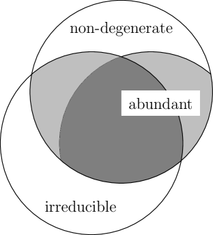
Figure 1.

With these clarifications made, we can illustrate the relation between the two varieties geometrically as sketched in Figure 2: Denote by $F_{n_{1},n_{2}}\bigl{(}\mathcal{K}(M)\bigr{)}$ the flag variety of inclusions $U_{1}\subset U_{2}\subset\mathcal{K}(M)$ of subspaces $U_{1}$ and $U_{2}$ in the space of Killing tensors with dimensions $\dim U_{1}=n_{1}=2n-1$ and $\dim U_{2}=n_{2}=\frac{1}{2}n(n+1)$. Forgetting either one of these two subspaces, we have the two projections

$$\pi_{i} :F_{n_{1},n_{2}}\bigl{(}\mathcal{K}(M)\bigr{)}\longrightarrow G_{n_{i}}\bigl{(}\mathcal{K}(M)\bigr{)} i =1,2$$

onto the corresponding Grassmannians. Denote by $\mathcal{I}\subseteq\mathcal{S}$ the set of irreducible non-degenerate superintegrable systems. In Section 6 we have shown that its image under the canonical map

$$\Phi_{1}:\mathcal{I}\longrightarrow G_{n_{1}}\bigl{(}\mathcal{K}(M)\bigr{)}$$

is a quasi-projective variety. In the same way, we can define a canonical map

$$\Phi_{2}:\mathcal{A}\longrightarrow G_{n_{2}}\bigl{(}\mathcal{K}(M)\bigr{)}$$

from the set $\mathcal{A}\subseteq\mathcal{S}$ of abundant non-degenerate superintegrable systems to the Grassmannian $G_{n_{2}}\bigl{(}\mathcal{K}(M)\bigr{)}$, by mapping such a system to the space spanned by all its linearly independent Killing tensors.

Figure 2.

As we are going to see shortly, the structure tensor $T_{ijk}$ of an abundant system can be obtained from its image under $\Phi_{2}$ by solving the prolongation equation (5.2) for $T_{ijk}$. The potential can then be recovered by integrating the prolongation (4.1). That is, an explicit knowledge of the set $\Phi_{2}(\mathcal{A})$ solves the classification problem for abundant non-degenerate superintegrable systems. This motivates the following definition.

Definition 7.18.

We call the subset

$$\Phi_{2}(\mathcal{A})\subset G_{\frac{n(n+1)}{2}}\bigl{(}\mathcal{K}(M)\bigr{)}$$

the classification space for abundant non-degenerate superintegrable systems.

Note that for abundant systems we have a fibre bundle

$$\Phi_{1}(\mathcal{A})\longrightarrow\Phi_{2}(\mathcal{A}),$$

whose fibres consist of superintegrable systems possessing the same structure tensor and are isomorphic to the Grassmannian $G_{n_{1}}(n_{2})$.

We are now ready to state our second main result.

Theorem 7.19.

The classification space for abundant non-degenerate superintegrable systems on a Riemannian manifold $M$ is a subvariety in the Grassmannian $G_{\frac{n(n+1)}{2}}\bigl{(}\mathcal{K}(M)\bigr{)}$ of $n(n+1)/2$-dimensional subspaces in the space $\mathcal{K}(M)$ of Killing tensors on $M$. It is isomorphic to the variety of cubic forms

$$\Psi_{ijk}x^{i}x^{j}x^{k}$$

on $\mathbb{R}^{n}$ satisfying

$$\young(j,k)\left(\Psi\indices{{}^{a}_{ij}}\Psi_{akl}+\frac{R}{n(n-1)}g_{ij}g_{kl}\right)=0.$$ (7.14)

Proof.

For a fixed point $x_{0}\in M$, let $Y$ be the variety of cubic forms on $T_{x_{0}}M\cong\mathbb{R}^{n}$ satisfying (7.14).

We construct the isomorphism $f:Y\to\Phi_{2}(\mathcal{A})$ from a map

$$\operatorname{Sym}^{3}T_{x_{0}}M\times\operatorname{Sym}^{2}T_{x_{0}}M\to\mathcal{K}(M),$$

sending a pair $(\Psi,S)$ to the Killing tensor $K\in\mathcal{K}(M)$ with

• $K_{ij}(x_{0})=S_{ij}$,

• $K_{ij,k}(x_{0})$ given by (5.2) and

• $K_{ij,kl}(x_{0})$ given by (5.6), with

• $T_{ijk}(x_{0})$ given by (7.6) with $B_{ijk}(x_{0})=\Psi$ and $C(x_{0})=0$ and

• $T_{ijk,l}(x_{0})$ given by (5.10).

This map is linear in $S$ and polynomial in $\Psi$ and hence defines a regular map $f:Y\to G_{n_{2}}(\mathcal{K}(M))$. Corollary 7.14 assures that its image lies in $\Phi_{2}(\mathcal{A})$.

The inverse of $f$ is a regular map $\Phi_{2}(\mathcal{A})\to Y$, constructed as follows. Consider a point $U_{2}\in\Phi_{2}(\mathcal{A})$, i.e. a subspace $U_{2}\subset\mathcal{K}(M)$ spanned by $n_{2}$ linearly independent Killing tensors $K^{(\alpha)}$ of an abundant system. Contracting $(i,j)$ in (5.2), one obtains

$$K^{ab}\tilde{T}_{abk}=K\indices{{}^{a}_{a,k}}$$ (7.15)

with

$$\tilde{T}_{ijk}=\frac{1}{3}\young(ij)\bigl{(}g_{kj}t_{i}-T_{kji}\bigr{)}.$$

The definition of $\tilde{T}_{ijk}$ implies

$$g^{ij}\tilde{T}_{ijk} =0 s_{i} :=g^{jk}\tilde{T}_{ijk}=\frac{n}{3}t_{k}.$$

Using (4.4a), we can express $T_{ijk}$ linearly in $\tilde{T}_{ijk}$ as

$$T_{kji}=\frac{3}{2}\left(\frac{n-2}{n(n-1)}s_{i}g_{jk}+\frac{1}{n-1}s_{j}g_{ik}-\tilde{T}_{ijk}\right).$$

Taking Equation (7.15) for each of the $K^{(\alpha)}$, we obtain a linear system of the form

$$AX=B,$$

where

• $A$ is the $n_{2}\!\times\!n_{2}$ -matrix whose rows contain the components $K_{ij}^{(\alpha)}$,

• $B$ is the $n_{2}\!\times\!n$ -matrix whose rows contain the components $g^{ab}K^{(\alpha)}_{ab,k}$ and

• $X$ the $n_{2}\!\times\!n$ -matrix containing the components $\tilde{T}_{ijk}$.

The matrix $A$ is invertible. Indeed, if the Killing tensors $K^{(\alpha)}$ are linearly dependent at some point $x$, then they are linearly dependent in $\mathcal{K}(M)$ by Proposition 5.5, which is a contradiction. Therefore the components $\tilde{T}_{ijk}$, given by

$$X=A^{-1}B=\frac{(\operatorname{Adj}A)B}{\det A},$$

are rational in $K^{(\alpha)}_{ij}$ and $K^{(\alpha)}_{ij,k}$. Since the Codazzi tensor $B_{ijk}$ is linear in $T_{ijk}$, which in turn is linear in $\tilde{T}_{ijk}$, the same is true for $B_{ijk}$. Note that derivatives and evaluation are linear operations, so that $K^{(\alpha)}_{ij}(x_{0})$ and $K^{(\alpha)}_{ij,k}(x_{0})$ are linear functions on $\mathcal{K}(M)$. Consequently, the components $B_{ijk}(x_{0})$ are rational functions on $\mathcal{K}(M)^{n_{2}}$ with non-vanishing denominator on the Stiefel manifold $V_{n_{2}}\bigl{(}\mathcal{K}(M)\bigr{)}$. Since the construction is independent of the choice of the basis $K^{(\alpha)}$ in the subspace $U_{2}$, these functions descend to regular functions on the Grassmannian $G_{n_{2}}(\mathcal{K}(M))$. This defines a regular map $G_{n_{2}}(\mathcal{K}(M))\to\operatorname{Sym}^{3}T_{x_{0}}M$, mapping the subspace spanned by the $n_{2}$ Killing tensors $K^{(\alpha)}$ to the cubic $\Psi_{ijk}=\frac{1}{3}B_{ijk}(x_{0})$. By Corollary 7.14 it restricts to a map $\Phi_{2}(\mathcal{A})\to Y$. ∎

8. Examples

Families of non-degenerate second-order superintegable systems
in arbitrary dimension $n\geqslant 3$

Euclidean geometry $g=\sum_{i}dx_{i}^{2}$	Complex $n$-sphere $g=-n(n-1)\,\sum_{i=1}^{n}\frac{dy_{i}^{2}}{y_{n}^{2}}=\sum_{i=0}^{n}dx_{i}^{2}$ (ambient coordinates $x_{i}$ on $\mathbb{R}^{n+1}\supset\mathbb{S}^{n}$)
Isotropic harmonic oscillator $V=\omega^{2}\,\sum_{i}x_{i}^{2}+\sum_{i}\alpha_{i}x_{i}$ $B=0$ mod gauge $\bar{t}=0$	—
Smorodinsky-Winternitz I	Smorodinsky-Winternitz I’
$V=\sum_{i=1}^{n}\left(\frac{a_{i}}{x_{i}^{2}}+\omega^{2}\,x_{i}^{2}\right)$	$V=-\frac{y_{n}^{2}}{n(n-1)}\sum_{i=1}^{n}\biggl{(}\frac{a_{i}}{y_{i}^{2}}+\omega^{2}y_{i}^{2}\biggr{)}$
$B=-\frac{3}{n-1}\,\sum_{i}(x_{i}^{2}\ln x_{i})$ mod gauge	$B=\frac{3n(n-1)}{2y_{n}^{2}}\sum_{i=1}^{n}(y_{i}^{2}\ln y_{i})$ mod gauge
$\bar{t}=-\frac{3}{n+2}\,\sum_{k}\ln x_{k}$	$\bar{t}=\frac{3}{n+2}\,\left((n+1)\ln x_{n}-\sum_{i\neq n}\ln x_{i}\right)$
Smorodinsky-Winternitz II	Smorodinsky-Winternitz II’
$V=\sum_{i\in J}(4\omega^{2}x_{i}^{2}+a_{i}x_{i})$ $+\sum_{i\in J^{c}}\biggl{(}\frac{a_{i}}{x_{i}^{2}}+\omega^{2}x_{i}^{2}\biggr{)}$	$V=-\frac{\,y_{n}^{2}}{n(n-1)}\Biggl{[}\sum_{i\in J}\Bigl{(}4\omega^{2}y_{i}^{2}+a_{i}y_{i}\Bigr{)}$ $+\sum_{i\in J^{c}}\biggl{(}\omega^{2}y_{i}^{2}+\frac{a_{i}}{y_{i}^{2}}\biggr{)}\Biggr{]}$
$B=-\frac{3}{n-1}\sum_{i\in J^{c}}x_{i}^{2}\ln x_{i}$ mod gauge	$B=\frac{3n(n-1)}{2y_{n}^{2}}\sum_{i\in J^{c}}y_{i}^{2}\ln y_{i}$ mod gauge
$\bar{t}=-\frac{3}{n+2}\,\sum_{i\in J^{c}}\ln x_{i}$	$\bar{t}=\frac{3}{n+2}\,\left((n+2)\ln y_{n}-\sum_{i\in J^{c}}\ln y_{i}\right)$
—	Generic system on the $n$-sphere $V=\sum_{i=0}^{n}\frac{a_{i}}{x_{i}^{2}}$ $B=-\frac{3}{2}\sum_{i=0}^{n}x_{i}^{2}\ln x_{i}$ mod gauge $\bar{t}=-\frac{3}{n+2}\,\sum_{i=0}^{n}\ln(x_{i})$

Table 2. Overview of examples discussed in the text. Examples in the same row are Stäckel equivalent. Note that the potential $V$ is stated up to an additive constant, and $B$ up to gauge terms. All examples are abundant with gauge choice $C=0$.

Arbitrary-dimensional families of superintegrable systems can be obtained by generalising low-dimensional examples, and subsequently through Bôcher contractions and Stäckel transforms. In the following we list some important families of superintegrable systems in arbitrary dimension, cf. Table 2. For each system we detail its potential $V$ (omitting the additive constant) and its structure function $B$ in a gauge where $C=0$ (all examples in the list are abundant in particular).

On flat space we use standard coordinates $x_{i}$. On the $n$-sphere, in order to make the similarity between the flat and the curved case apparent, we use local coordinates $y_{i}$ with

$$g=-n(n-1)\sum_{i=1}^{n}\frac{dy_{i}^{2}}{y_{n}^{2}},$$

except for the generic system, which we write in the coordinates $x_{i}$ of the ambient Euclidean space.

8.1. Isotropic harmonic oscillator.

$$V =\sum_{i=1}^{n}(\omega^{2}x_{i}^{2}+a_{i}x_{i}) B =0$$

This is the trivial case already mentioned in Example 3.6. Its structure tensor vanishes and therefore, up to gauge terms, all its structure functions vanish as well.

8.2. Smorodinsky-Winternitz I

$$V =\sum_{i=1}^{n}\biggl{(}\frac{a_{i}}{x_{i}^{2}}+\omega^{2}x_{i}^{2}\biggr{)} B =-\frac{3}{n-1}\sum_{i=1}^{n}x_{i}^{2}\ln x_{i}$$

This system was first described on flat space by Friš et al. [FMS⁺65] and is often called the “generic system on flat space”. For low dimensions, other labels have also been used in the literature such as $(0,11,0)$ in [KS19] or [E1] in [KKPM01]. The corresponding label in three dimensions is [I] in [KKM06a, KKM07c, Cap14].

This system has a Stäckel invariant counterpart on the $n$-sphere, known as [I’] in dimension three [KKM07c]:

$$V =-\frac{y_{n}^{2}}{n(n-1)}\sum_{i=1}^{n}\biggl{(}\frac{a_{i}}{y_{i}^{2}}+\omega^{2}y_{i}^{2}\biggr{)} B =\frac{3n(n-1)}{2y_{n}^{2}}\sum_{i=1}^{n}y_{i}^{2}\ln y_{i}$$

8.3. Smorodinsky-Winternitz II

$$V =\sum_{i\in J}(4\omega^{2}x_{i}^{2}+a_{i}x_{i})+\sum_{i\in J^{c}}\biggl{(}\frac{a_{i}}{x_{i}^{2}}+\omega^{2}x_{i}^{2}\biggr{)} B =-\frac{3}{n-1}\sum_{i\in J^{c}}x_{i}^{2}\ln x_{i}$$

In dimension $2$, this system is also denoted by $(0,1,0)$ [KS19] or [E2] in [KKPM01]. In dimension $3$, it is labeled [IV] [KKM06a]. This system formally appears as a superposition of the Smorodinski-Winternitz system I and the isotropic harmonic oscillator, defined by a partition of the index set,

$$\{1,2,\ldots,n\}=J\cup J^{c}.$$

This might be an indication for the existence of a composition of superintegrable systems similarly to the operad construction of separable systems on spheres [SV15].

The corresponding system on the $n$-sphere reads

$$V =-\frac{\,y_{n}^{2}}{n(n-1)}\Biggl{[}\sum_{i\in J}\Bigl{(}4\omega^{2}y_{i}^{2}+a_{i}y_{i}\Bigr{)}+\sum_{i\in J^{c}}\biggl{(}\omega^{2}y_{i}^{2}+\frac{a_{i}}{y_{i}^{2}}\biggr{)}\Biggr{]}$$

$$B =\frac{3n(n-1)}{2y_{n}^{2}}\sum_{i\in J^{c}}y_{i}^{2}\ln y_{i}$$

In low dimensions, the labels [S1] [KKPM01] and [IV’] [KKM06a, Cap14] have been used for this system.

8.4. The generic system on the $n$-sphere

$$V =\sum_{i=0}^{n}\frac{a_{i}}{x_{i}^{2}} B =-\frac{3}{2}\sum_{i=0}^{n}x_{i}^{2}\ln x_{i}$$

This system on the $n$-sphere, not to be confused with the generic system on flat space, is labelled [S9] for 2D in [KKPM01] and [VIII] in [KKM07c, KKM06a] for 3D. Its name and its significance result from the fact that in dimensions two and three any other non-degenerate second-order superintegrable system can be obtained from it via Stäckel transforms and contractions.

Note that the term “generic” has a precise meaning in our algebraic geometric context: it refers to a Zariski open subset in the classification space. We remark that if the latter turns out to be reducible, there might as well be several “generic” systems, as observed for the Euclidean plane [KS19].

References

- [ADS06] Maria A. Agrotis, Pantelis A. Damianou, and Christodoulos Sophocleous, The Toda lattice is super-integrable, Physica A: Statistical Mechanics and its Applications 365 (2006), no. 1, 235 – 243, Fundamental Problems of Modern Statistical Mechanics.
- [AS] Milton Abramowitz and Irene A. Stegun (eds.), Handbook of mathematical functions with formulas, graphs, and mathematical tables, Dover books on elementary and intermediate mathematics, XIV-1046 p. : FIG.
- [Ask85] R. Askey, Continuous Hahn polynomials, J. Phys. A 18 (1985), no. 16, L1017–L1019.
- [AW85] R. Askey and J. Wilson, Some basic hypergeometric orthogonal polynomials that generalize Jacobi polynomials, Mem. Amer. Math. Soc. 54 (1985), no. 319, iv+55.
- [Bat53] Harry Bateman, Higher transcendental functions, vol. I–III, McGraw-Hill, New York, 1953, https://authors.library.caltech.edu/43491/.
- [Bat54] by same author, Tables of integral transforms, vol. I–II, McGraw-Hill, New York, 1954, https://authors.library.caltech.edu/43489/.
- [BCG+13] R.L. Bryant, S.S. Chern, R.B. Gardner, H.L. Goldschmidt, and P.A. Griffiths, Exterior differential systems, Mathematical Sciences Research Institute Publications, Springer New York, 2013.
- [BCLO11] Ronald Boisvert, Charles W. Clark, Daniel Lozier, and Frank Olver, A special functions handbook for the digital age, Notices of the AMS (2011), 905–911.
- [BDK93] D. Bonatsos, C. Daskaloyannis, and K. Kokkotas, Quantum-algebraic description of quantum superintegrable systems in two dimensions, Phys. Rev. A (3) 48 (1993), no. 5, R3407–R3410.
- [BH09] Ángel Ballesteros and Francisco J Herranz, Maximal superintegrability of the generalized kepler–coulomb system onN-dimensional curved spaces, Journal of Physics A: Mathematical and Theoretical 42 (2009), no. 24, 245203.
- [BKM86] C. P. Boyer, E. G. Kalnins, and W. Miller, Jr., Stäckel-equivalent integrable hamiltonian systems, SIAM Journal on Mathematical Analysis 17 (1986), no. 4, 778–797.
- [Cap14] Joshua J. Capel, Classification of second-order conformally-superintegrable systems, Ph.D. thesis, PhD Thesis, School of Mathematics and Statistics, University of New South Wales, 2014.
- [CK14] J. J. Capel and J. M. Kress, Invariant classification of second-order conformally flat superintegrable systems, J. Phys. A 47 (2014), no. 49, 495202, 33.
- [CKP15] Joshua J. Capel, Jonathan M. Kress, and Sarah Post, Invariant classification and limits of maximally superintegrable systems in 3d, Symmetry, Integrability and Geometry: Methods and Applications (2015).
- [DLMF] NIST Digital Library of Mathematical Functions, http://dlmf.nist.gov/, Release 1.0.24 of 2019-09-15, F. W. J. Olver, A. B. Olde Daalhuis, D. W. Lozier, B. I. Schneider, R. F. Boisvert, C. W. Clark, B. R. Miller, B. V. Saunders, H. S. Cohl, and M. A. McClain, eds.
- [DT07] C. Daskaloyannis and Y. Tanoudis, Quantum superintegrable systems with quadratic integrals on a two dimensional manifold, J. Math. Phys. 48 (2007), no. 7, 072108, 22.
- [DTGVL05] Gema M. Diaz-Toca, Laureano Gonzalez-Vega, and Henri Lombardi, Generalizing Cramer’s rule: Solving uniformly linear systems of equations, SIAM Journal on Matrix Analysis and Applications 27 (2005), no. 3, 621–637.
- [DY06] C. Daskaloyannis and K. Ypsilantis, Unified treatment and classification of superintegrable systems with integrals quadratic in momenta on a two-dimensional manifold, J. Math. Phys. 47 (2006), no. 4, 042904, 38.
- [ERMS17] Mauricio A. Escobar Ruiz, Willard Miller, Jr., and Eyal Subag, Contractions of degenerate quadratic algebras, abstract and geometric, SIGMA Symmetry Integrability Geom. Methods Appl. 13 (2017), Paper No. 099, 32. MR 3740337
- [Fer81] Dirk Ferus, A remark on codazzi tensors in constant curvature spaces, Lecture Notes in Mathematics, vol. 838, p. 257, Springer-Verlag, 1981.
- [FH00] William Fulton and Joe Harris, Representation theory: A first course, springer study edition ed., Graduate Texts in Mathematics, no. 129, Springer-Verlag, 2000.
- [FMS+65] J. Friš, V. Mandrosov, Ya.A. Smorodinsky, M. Uhlíř, and P. Winternitz, On higher symmetries in quantum mechanics, Physics Letters 16 (1965), no. 3, 354 – 356.
- [Ful97] William Fulton, Young tableaux: With applications to representation theory and geometry, London Mathematical Society Student Texts, no. 35, Cambridge University Press, 1997.
- [GIVZ13] Vincent X Genest, Mourad E H Ismail, Luc Vinet, and Alexei Zhedanov, The Dunkl oscillator in the plane: I. Superintegrability, separated wavefunctions and overlap coefficients, Journal of Physics A: Mathematical and Theoretical 46 (2013), no. 14, 145201.
- [GL19] A. Rod Gover and Thomas Leistner, Invariant prolongation of the Killing tensor equation, Ann. Mat. Pura Appl. (4) 198 (2019), no. 1, 307–334. MR 3918632
- [Gol67] Hubert Goldschmidt, Integrability criteria for systems of nonlinear partial differential equations, J. Differential Geom. 1 (1967), no. 3-4, 269–307.
- [Gra04] Simon Gravel, Hamiltonians separable in cartesian coordinates and third-order integrals of motion, Journal of Mathematical Physics 45 (2004), 1003–1019.
- [GVZ14] Vincent X. Genest, Luc Vinet, and Alexei Zhedanov, Interbasis expansions for the isotropic 3D harmonic oscillator and bivariate Krawtchouk polynomials, J. Phys. A 47 (2014), no. 2, 025202, 13. MR 3150528
- [HGDR84] J. Hietarinta, B. Grammaticos, B. Dorizzi, and A. Ramani, Coupling-constant metamorphosis and duality between integrable hamiltonian systems, Phys. Rev. Lett. 53 (1984), 1707–1710.
- [HMPZ18] Md. Fazlul Hoque, Ian Marquette, Sarah Post, and Yao-Zhong Zhang, Algebraic calculations for spectrum of superintegrable system from exceptional orthogonal polynomials, Annals of Physics 391 (2018), 203 – 215.
- [IW53] E. Inönü and E.P. Wigner, On the contraction of groups and their representations, Proc. Nat. Acad. Sci. USA 39 (1953), 510–524.
- [Kal86] Ernest G. Kalnins, Separation of variables for Riemannian spaces of constant curvature, Pitman Monographs and Surveys in Pure and Applied Mathematics, vol. 28, Longman Scientific & Technical, Harlow, England, 1986.
- [KJS16a] Ernie G. Kalnins, Willard Miller Jr., and Eyal Subag, Bôcher contractions of conformally superintegrable Laplace equations, SIGMA 12 (2016), no. 038, 31 pages.
- [KJS16b] by same author, Laplace equations, conformal superintegrability and Bôcher contractions, Acta Polytechnica 56 (2016), no. 3, 214–223.
- [KK02] J. M. Kress and E. G. Kalnins, Multiseparability and superintegrability in three dimensions, Phys. Atomic Nuclei 65 (2002), no. 6, 1047–1051, Symposium on Integrable Systems (Dubna, 2000).
- [KKM05a] E. G. Kalnins, J. M. Kress, and W. Miller, Jr., Second-order superintegrable systems in conformally flat spaces. I. Two-dimensional classical structure theory, J. Math. Phys. 46 (2005), no. 5, 053509, 28.
- [KKM05b] by same author, Second order superintegrable systems in conformally flat spaces. II. The classical two-dimensional Stäckel transform, J. Math. Phys. 46 (2005), no. 5, 053510, 15.
- [KKM05c] by same author, Second order superintegrable systems in conformally flat spaces. III. Three-dimensional classical structure theory, J. Math. Phys. 46 (2005), no. 10, 103507, 28.
- [KKM06a] by same author, Second order superintegrable systems in conformally flat spaces. IV. The classical 3D Stäckel transform and 3D classification theory, J. Math. Phys. 47 (2006), no. 4, 043514, 26.
- [KKM06b] by same author, Second-order superintegrable systems in conformally flat spaces. V. Two- and three-dimensional quantum systems, J. Math. Phys. 47 (2006), no. 9, 093501, 25.
- [KKM07a] by same author, Fine structure for 3D second-order superintegrable systems: three-parameter potentials, J. Phys. A 40 (2007), no. 22, 5875–5892.
- [KKM07b] by same author, Nondegenerate 2D complex Euclidean superintegrable systems and algebraic varieties, J. Phys. A 40 (2007), no. 13, 3399–3411.
- [KKM07c] by same author, Nondegenerate three-dimensional complex Euclidean superintegrable systems and algebraic varieties, J. Math. Phys. 48 (2007), no. 11, 113518, 26.
- [KKM18] Ernest G Kalnins, Jonathan M Kress, and Willard Miller, Separation of variables and superintegrability, 2053-2563, IOP Publishing, 2018.
- [KKMP07] E. G. Kalnins, J. M. Kress, W. Miller, and G. S. Pogosyan, Nondegenerate superintegrable systems in n-dimensional euclidean spaces, Physics of Atomic Nuclei 70 (2007), no. 3, 545–553.
- [KKMP09] E. G. Kalnins, J. M. Kress, W. Miller, Jr., and S. Post, Structure theory for second order 2D superintegrable systems with 1-parameter potentials, SIGMA Symmetry Integrability Geom. Methods Appl. 5 (2009), 008, 24.
- [KKMW03] E. G. Kalnins, J. M. Kress, W. Miller, Jr., and P. Winternitz, Superintegrable systems in Darboux spaces, J. Math. Phys. 44 (2003), no. 12, 5811–5848.
- [KKPM01] E. G. Kalnins, J. M. Kress, G. S. Pogosyan, and W. Miller, Jr., Completeness of multiseparable superintegrability in two-dimensional constant curvature spaces, Journal of Physics A: Mathematical and General 34 (2001), 4705–4720.
- [KKW02] E. G. Kalnins, J. M. Kress, and P. Winternitz, Superintegrability in a two-dimensional space of nonconstant curvature, J. Math. Phys. 43 (2002), no. 2, 970–983.
- [KLV86] I.S. Krasil’ščik, V.V. Lychagin, and A.M. Vinogradov, Geometry of jet spaces and nonlinear partial differential equations, Advanced studies in contemporary mathematics, Gordon and Breach Science Publishers, 1986.
- [KM86] Ernest G. Kalnins and Willard Miller Jr., Separation of variables on -dimensional Riemannian manifolds. I. The -sphere and Euclidean -space , Journal of Mathematical Physics 27 (1986), no. 7, 1721–1736.
- [KMP00a] E. G. Kalnins, W. Miller, Jr., and G. S. Pogosyan, Completeness of multiseparable superintegrability in , J. Phys. A 33 (2000), no. 22, 4105–4120.
- [KMP00b] by same author, Completeness of multiseparable superintegrability on the complex 2-sphere, J. Phys. A 33 (2000), no. 38, 6791–6806.
- [KMP07] E. G. Kalnins, W. Miller, Jr., and S. Post, Wilson polynomials and the generic superintegrable system on the 2-sphere, J. Phys. A 40 (2007), no. 38, 11525–11538.
- [KMP11] Ernie G. Kalnins, Willard Miller, Jr., and Sarah Post, Two-variable Wilson polynomials and the generic superintegrable system on the 3-sphere, SIGMA Symmetry Integrability Geom. Methods Appl. 7 (2011), Paper 051, 26. MR 2804585
- [KMP13] E. G. Kalnins, W. Miller, Jr., and S. Post, Contractions of 2D 2nd order quantum superintegrable systems and the Askey scheme for hypergeometric orthogonal polynomials, SIGMA Symmetry Integrability Geom. Methods Appl. 9 (2013), 057, 28.
- [Koo09] T. H. Koornwinder, The Askey scheme as a four-manifold with corners, Ramanujan Journal. An International Journal Devoted to the Areas of Mathematics Influenced by Ramanujan 20 (2009), no. 3, 409–439.
- [Kre07] J. M. Kress, Equivalence of superintegrable systems in two dimensions, Physics of Atomic Nuclei 70 (2007), no. 3, 560–566.
- [KS19] Jonathan Kress and Konrad Schöbel, An algebraic geometric classification of superintegrable systems in the euclidean plane, Journal of Pure and Applied Algebra 223 (2019), no. 4, 1728–1752.
- [MPR20] Ian Marquette, Sarah Post, and Lisa Ritter, A fourth-order superintegrable system with a rational potential related to painlevé VI, Journal of Physics A: Mathematical and Theoretical 53 (2020), no. 50, 50LT01.
- [MPW13] W. Miller, Jr., S. Post, and P. Winternitz, Classical and quantum superintegrability with applications, J. Phys. A 46 (2013), no. 42, 423001, 97.
- [Nie79] Michael Martin Nieto, Hydrogen atom and relativistic pi-mesic atom in n-space dimensions, American Journal of Physics 47 (1979), no. 12, 1067–1072.
- [Pee06] Kasper Peeters, A field-theory motivated approach to symbolic computer algebra, Computer Physics Communications 176 (2006), no. 8, 550–558, arXiv:cs/0608005 [cs.SC].
- [Pee07] by same author, Introducing Cadabra: a symbolic computer algebra system for field theory problems, 2007, arXiv:hep-th/0701238.
- [Pos10] Sarah Post, Coupling constant metamorphosis, the stäckel transform and superintegrability, AIP Conference Proceedings 1323 (2010), no. 1, 265–274.
- [PP90] J. F. Plebański and M. Przanowski, The -dimensional classical Kepler’s problem “without integration”, Rev. Mexicana Fís. 36 (1990), no. 3, 465–470. MR 1070683
- [Ptory] Claudius Ptolemy, Almagest, vol. I, Alexandria, 2nd century.
- [PTV12] Sarah Post, Satoshi Tsujimoto, and Luc Vinet, Families of superintegrable hamiltonians constructed from exceptional polynomials, Journal of Physics A: Mathematical and Theoretical 45 (2012), no. 40, 405202.
- [RKWMS17] M. A. Escobar Ruiz, E. G. Kalnins, Jr. W. Miller, and E. Subag, Bôcher and abstract contractions of 2nd order quadratic algebras, SIGMA 13 (2017), no. 013, 38 pages.
- [Sch12] Konrad Schöbel, Algebraic integrability conditions for Killing tensors on constant sectional curvature manifolds, Journal of Geometry and Physics 62 (2012), no. 5, 1013–1037.
- [Sch14] by same author, The variety of integrable Killing tensors on the 3-sphere, SIGMA 10 (2014), no. 080, 48 pages, arxiv:1205.6227.
- [Sch15] by same author, An algebraic geometric approach to separation of variables, Research Series, Springer Spektrum, 2015.
- [Sch16] by same author, Are orthogonal separable coordinates really classified?, SIGMA 12 (2016), no. 041, 16 pages, arxiv:1510.09028.
- [SV15] Konrad Schöbel and Alexander P. Veselov, Separation coordinates, moduli spaces and Stasheff polytopes, Communications in Mathematical Physics 337 (2015), no. 3, 1255–1274.
- [Tem04] P. Tempesta, On superintegrable systems in : algebraic properties and symmetry preserving discretization, Superintegrability in classical and quantum systems, CRM Proc. Lecture Notes, vol. 37, Amer. Math. Soc., Providence, RI, 2004, pp. 223–239.
- [Wil07] E. J. Wilczynski, Projective differential geometry of curved surfaces. I, Trans. Amer. Math. Soc. 8 (1907), no. 2, 233–260. MR 1500783
- [Wil09] by same author, Projective differential geometry of curved surfaces. IV, Trans. Amer. Math. Soc. 10 (1909), no. 2, 176–200. MR 1500833
- [Win04] P. Winternitz, Superintegrable systems in classical and quantum mechanics, New trends in integrability and partial solvability, NATO Sci. Ser. II Math. Phys. Chem., vol. 132, Kluwer Acad. Publ., Dordrecht, 2004, pp. 281–297.
- [WMT] Stephen Wolfram, Oleg Marichev, and Michael Trott, The Mathematical Functions Site, online database, http://functions.wolfram.com/.
- [Woj83] S. Wojciechowski, Superintegrability of the calogero-moser system, Physics Letters A 95 (1983), no. 6, 279 – 281.
- [Wol98] Thomas Wolf, Structural equations for Killing tensors of arbitrary rank, Computer Physics Communications 115 (1998), no. 2–3, 316–329.