Shape Reconstruction by Learning Differentiable Surface Representations

Abstract

Generative models that produce point clouds have emerged as a powerful tool to represent 3D surfaces, and the best current ones rely on learning an ensemble of parametric representations. Unfortunately, they offer no control over the deformations of the surface patches that form the ensemble and thus fail to prevent them from either overlapping or collapsing into single points or lines. As a consequence, computing shape properties such as surface normals and curvatures becomes difficult and unreliable.

In this paper, we show that we can exploit the inherent differentiability of deep networks to leverage differential surface properties during training so as to prevent patch collapse and strongly reduce patch overlap. Furthermore, this lets us reliably compute quantities such as surface normals and curvatures. We will demonstrate on several tasks that this yields more accurate surface reconstructions than the state-of-the-art methods in terms of normals estimation and amount of collapsed and overlapped patches.

Figure 1: Our method allows for prediction of multi-patch representation where the patches are guaranteed not to collapse and to minimize the overlap. Thanks to explicit access to the differentiable surface properties, our method computes normals and curvature analytically for any predicted point of the modeled surface.

1 Introduction

Point clouds are becoming increasingly popular as a compact and expressive way to represent 3D surfaces because they can capture high frequency geometric details without requiring much memory. State-of-the-art methods rely on encoder/decoder architectures to create latent representations from input data and then decode them using one or more learned mappings from a 2D parameter space to the 3D surface. Each one of these mappings can be thought of as transforming a 2D rectangular patch into a set of 3D points lying on the surface to be modeled. FoldingNet [34] and AtlasNet [16] are among the best representatives of this approach, and the move from one single patch to multiple ones has proved effective to achieve higher accuracy.

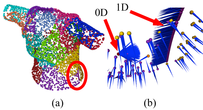
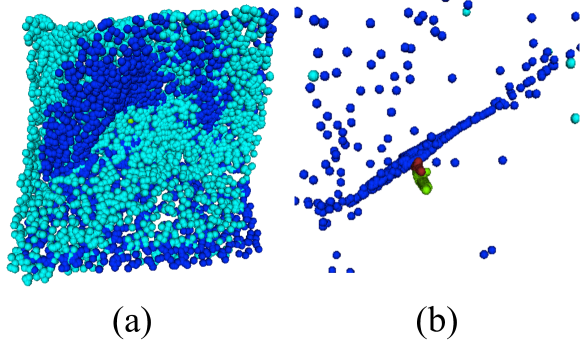
However, this increase in accuracy comes at a price. Nothing guarantees that each patch will represent a substantial portion of the target surface and some may in fact collapse, meaning that they generate a single point or a line instead of a surface-like cloud. Another potential problem is that the 3D clouds generated by different patches will overlap so that the same parts of the underlying surface are represented by several patches, thus resulting in potential inconsistencies across the patches and ineffectively using the decoder’s capacity. While these problems may not occur when the training data contains many diverse categories of objects, such as when using the whole of ShapeNet dataset [10], they become apparent in practical scenarios where one aims to model the shape of a specific surface, such as a piece of clothing, as shown in Fig. 1.

In this paper, we address these two issues by leveraging the observation that first and second derivatives of the decoder output can be used to compute the differential properties of the reconstructed surface, without having to triangulate it. In other words, we can compute exact surface properties analytically, rather than having to approximate these quantities using the point cloud or a mesh. This enables us to incorporate into our training loss function terms that prevent patch collapse and strongly reduce patch overlap.

In our experiments, we will show that being able to compute differential properties and to exploit them during training (1) fully prevents any type of patch collapse, (2) substantially reduces the amount of patch overlap (3) lets us predict surface normals with higher accuracy than SotA.

Our approach to exploiting differentiability is not tied to a specific architecture and we will show on several tasks that it yields not only state-of-the-art accuracy but but also a much better behaved surface representation whose differentiable properties can be estimated easily.

Our contribution is therefore a generic approach to leveraging 3D point cloud generating schemes so that the differential properties of the target surfaces are immediately available without further post-processing, which makes them usable by subsequent algorithms that require them to perform tasks such as shape-from-shading, texture mapping, surface normal estimation from range scans [2, 19], and detail-preserving re-meshing [8].

2 Related Work

Deep generative approaches for surface reconstruction.

Modern generative Deep Nets are very good at reconstructing 3D surfaces for tasks such as shape completion from incomplete data [11, 26, 30, 28], single-view shape reconstruction [16, 25, 6, 14], and auto-encoding point-clouds [16, 13]. They represent the surfaces in terms of voxels [33, 30, 15], triangular meshes [25, 6, 12], or point clouds [16, 13, 14]. The common denominator of all these methods is that they deliver precise shapes in terms of 3D locations but not necessarily in terms of differential surface properties, such as normals and curvature. The latter may be inaccurate and even nonsensical as will be shown in the experiment section.

Patch-based representations.

Among all these methods, FoldingNet [34] was the first to introduce the idea of learning a parametric mapping from a 2D patch to a 3D surface. It relies on a discrete sampling and follow-up methods introduced continuous multi-patch representations that are trained by minimizing the Chamfer distance [16, 13], a shape aware variant of the L2 distance [29], or are optimized to predict a single sample using Earth mover’s distance[32]. One of the biggest advantage of these approaches is that the learned mapping, being a continuous function, allows for arbitrary sampling resolution at test time. However, still none of these methods gives access to the differential surface properties. An exception is the approach of [21] that learns a parameterization for B-spline approximation but only works with 2D curves.

Using differential surface properties for training.

There are a few deep learning techniques that use differential surface properties in the form of either normal maps [6, 3] or their approximations computed on triangular meshes [17] but none that rely on 3D point clouds. Using differential surface properties still mostly belongs to the realm of non-deep learning methods, for example for shape from template [22, 5] or non-rigid structure-from-motion [1, 24], which are beyond the scope of this paper.

3 Multi Patch Representations

As discussed above, multi-patch representations [16, 32] are powerful tools for generating surfaces from latent representations. However, they suffer from a number of limitations that we discuss below and will address in Section 4.

3.1 Formalization

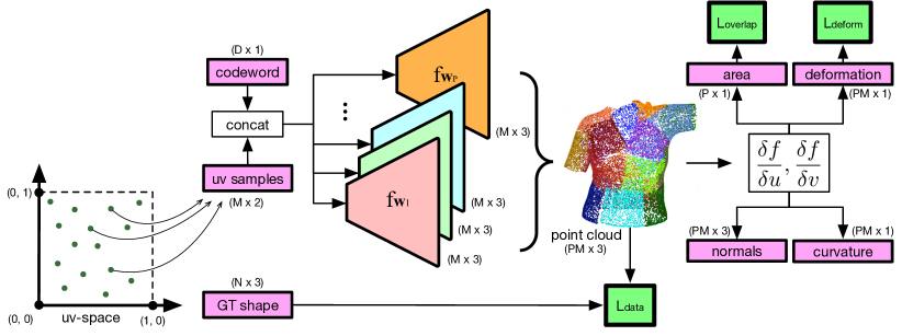
Let us consider a mapping $\mathcal{F}$ from a given low-dimensional latent vector $\mathbf{d}\in\mathbb{R}^{D}$ to a surface $\mathcal{S}$ in 3D space represented by a cloud of 3D points. In the multi-patch approach, the point cloud is taken to be the union of points generated by $K$ independent mappings $f_{\mathbf{w}_{k}}:~{}\mathbb{R}^{D}\times\mathcal{D}_{f}\rightarrow~{}\mathbb{R}^{3}$ for $1 \leq j\leq K$, where each $f_{\mathbf{w}_{k}}$ is a trainable network with parameters $\mathbf{w}_{k}$ and $\mathcal{D}_{f}=[c_{\text{min}},c_{\text{max}}]^{2}$ represents a square in $\mathbb{R}^{2}$. In other words, the $f_{\mathbf{w}_{k}}$ network takes as input a latent vector $\mathbf{d}$ and a 2D point in $\mathcal{D}_{f}$ and returns a 3D point.

Given a training set containing many 3D shapes, the $\mathbf{w}_{k}$ network weights are learned by minimizing a sum of chamfer-based losses, one for each 3D shape in a training batch, of the form

$$\begin{split}\mathcal{L}_{\text{CHD}}=&\frac{1}{KM}\sum_{k=1}^{K}\sum_{i=1}^{M}\min_{j}\left\lVert\mathbf{p}_{i}^{(k)}-\mathbf{q}_{j}\right\rVert^{2}+\\ &\frac{1}{N}\sum_{j=1}^{N}\min_{i,k}\left\lVert\mathbf{p}_{i}^{(k)}-\mathbf{q}_{j}\right\rVert^{2},\end{split}$$ (1)

where $M$ is the number of points predicted by each patch, $N$ is the number of GT points, $\mathbf{p}_{i}^{k}$ is the $i$-th 3D point predicted by $f_{\mathbf{w}_{k}}$, and $\mathbf{q}_{j}$ is the $j$-th GT point. The whole pipeline is depicted in Figure 4.

3.2 Limitations

Minimizing the loss function of Eq. 1 yields patches that jointly cover the whole surface but does not constrain how much deformation individual patches undergo or how they are positioned with respect to each other. In practice, this leads to two potential failure modes.

Figure 2: 2D representation of typical patch collapses. (a) 0D collapse, (b) 1D stretch collapse, (c) 1D skew collapse and (d) partial collapse.

Patch Collapse.

Some of the patches might collapse to undesirable configurations, such as those shown in Figure 2. This may not increase the total $\mathcal{L}_{\text{CHD}}$ value much when training is complete because the remaining, non-collapsed patches can compensate for the collapsed ones. However, collapsed patches still cause two main problems. First, their normals and curvature do not make sense anymore. Second, the $f_{\mathbf{w}_{j}}$ corresponding to a collapsed patch becomes useless, thus wasting the representational power of $\mathcal{F}$.

Patch Overlap.

Figure 3: Patch overlap. (a) Up to 3-fold overlap. (b) Configuration with small overlap.

Another drawback of this approach is that it provides no control over the relative spatial configuration of the patches. Thus, it does not prevent them from overlapping each other, as depicted by Figure 3. This is an undesirable behavior because the overlapping patches may yield surfaces that are not well aligned and, again, because some of the expressive power of $\mathcal{F}$ is wasted.

Figure 4: Schematic view of our approach. The input to the set of $K$ decoders $\{f_{\mathbf{w}_{k}}\}$ is a latent vector $\mathbf{d}$ (dubbed codeword) and a set of 2D points sampled from the domain ${\cal D}_{f}$ (dubbed uv-space). The decoders produce point clouds, which together represent the target surface. The derivatives of $f_{\mathbf{w}_{k}}$ w.r.t. the uv-space allow for the analytical computation of each patch’s area and deformation properties. The loss function used to train our model consists of a data term $\mathcal{L}_{\text{data}}$ using GT annotations and of terms $\mathcal{L}_{\text{ol}}$ and $\mathcal{L}_{\text{def}}$ which prevent patch overlap and patch collapse, respectively.

4 Accounting for Differential Properties

We have seen that multi-patch representations are powerful but are subject to patch collapse and overlap, both of which reduce their expressive power. We now show that by regularizing the differential properties of the reconstructed surfaces during training, we can eliminate patch collapse and mitigate patch overlap. We will demonstrate in Section 5 that this boosts the accuracy of normals and curvature.

In the remainder of this section, we first explain how we can compute online the differential properties of surfaces represented by a 3D point cloud. We then present our approach to using them during training.

4.1 Differential Surface Properties

Let $\mathbf{r}=[u,v]\in\mathcal{D}_{f}$, where $\mathcal{D}_{f}$ is the 2D domain over which $f_{\mathbf{w}_{k}}$ is defined, as explained at the beginning of Section 3.1. $\mathbf{p}=f_{\mathbf{w}_{k}}(\mathbf{r})$ is a point of surface $\mathcal{S}$. We can compute the differential properties of $\mathcal{S}$, including normals and curvatures, from the derivatives of $f_{\mathbf{w}_{k}}$ with respect to $u$ and $v$ as follows, given that $f_{\mathbf{w}_{k}}$ is a continuously differentiable function. For notational simplicity, we drop the subscript $\mathbf{w}_{k}$ from $f_{\mathbf{w}_{k}}$ in the remainder of this section.

Let $\mathbf{J}=\begin{bmatrix}\mathbf{f}_{u}&\mathbf{f}_{v}\end{bmatrix}$ be the Jacobian of $f$ at $\mathbf{p}$, where $\mathbf{f}_{u}=\frac{\partial f}{\partial u}$ and $\mathbf{f}_{v}=\frac{\partial f}{\partial v}$. The normal vector is

$$\mathbf{n}=\frac{\mathbf{f}_{u}\times\mathbf{f}_{v}}{\left\lVert\mathbf{f}_{u}\times\mathbf{f}_{v}\right\rVert}.$$ (2)

The curvature, area and deformation properties can be computed from the metric tensor

$$g=\mathbf{J}^{\top}\mathbf{J}=\begin{bmatrix}\mathbf{f}_{u}^{\top}\mathbf{f}_{u}&\mathbf{f}_{u}^{\top}\mathbf{f}_{v}\\ \mathbf{f}_{u}^{\top}\mathbf{f}_{v}&\mathbf{f}_{v}^{\top}\mathbf{f}_{v}\end{bmatrix}=\begin{bmatrix}E&F\\ F&G\end{bmatrix}.$$ (3)

The mean and Gaussian curvature are then

$$c_{\text{mean}} =-\frac{1}{2\det{g}}\mathbf{n}^{\top}\left[\frac{\partial^{2}f}{\partial u^{2}}G-2\frac{\partial^{2}f}{\partial u\partial v}F+\frac{\partial^{2}f}{\partial v^{2}}E\right],$$ (4)

$$c_{\text{gauss}} =\frac{\frac{\partial^{2}f}{\partial u^{2}}^{\top}\mathbf{n}\cdot\frac{\partial^{2}f}{\partial v^{2}}^{\top}\mathbf{n}-(\frac{\partial^{2}f}{\partial u\partial v}^{\top}\mathbf{n})^{2}}{EG-F^{2}}.$$ (5)

Furthermore, the area of the surface covered by the patch can be estimated as

$$A=\iint_{\mathcal{D}_{f}}{\sqrt{EG-F^{2}}dudv}.$$ (6)

Note that all these surface properties are computed analytically. Thus they are exact, differentiable, and do not require a triangulation. This is unlike traditional methods that approximate these quantities on a point cloud or a mesh.

4.2 Learning a Robust Mapping

Recall that our goal is to learn a mapping $\mathcal{F}$ from multiple 2D patches to a 3D point cloud. In particular, we seek to constrain the deformations modeled by $\mathcal{F}$ such that patch collapse is prevented but complex surfaces can still be represented accurately. We now discuss the deformation model that we rely on and then introduce the required training loss functions.

4.2.1 Deformation Model

Conformal mappings yield low distortions while retaining the capacity to model complex shapes. They are therefore widely used in computer graphics and computer vision, for example for texture mapping [9] and surface reconstruction [24]. For a surface to undergo conformal deformation, the metric tensor must be of the form

$$g_{\text{conf}}=s(\mathbf{r})\begin{bmatrix}1&0\\ 0&1\end{bmatrix},$$ (7)

where $s:\mathcal{D}_{f}\rightarrow\mathbb{R}$ returns a scale value for each position in the parameter space. Unfortunately, making the deformation conformal does not prevent patch collapse, even in a single-patch scenario, since partial collapse can still occur wherever $s(\mathbf{r}_{i})\sim 0$.

To address this, we propose to use fixed-scale conformal mappings whose metric tensors can be written as

$$g_{\text{fsconf}}=s\begin{bmatrix}1&0\\ 0&1\end{bmatrix},$$ (8)

where $s$ is an unknown global scale shared by all parameter space locations. Constraining $\mathcal{F}$ to be a fixed scale conformal mapping amounts to assuming that the target surface is patch-wise developable, which has proved to be a reasonable assumption in the domain of deformable surface reconstruction [5, 4, 23].

In a single patch scenario, $s\sim 0$ is not an option anymore when minimizing the loss of Eq. 1 because the resulting surface would be point-collapsed and thus could not cover the full target surface. However, collapses can still occur in the multi-patch case, and have to be prevented using appropriate loss terms, as discussed below.

4.2.2 Loss Functions

Here, we formulate the loss terms that should be added to the data loss $\mathcal{L}_{\text{CHD}}$ of Eq. 1 during training to ensure that the resulting $f_{\mathbf{w}_{k}}$ are fixed-scale conformal, as described above, without patch collapse, and with as little overlap as possible.

Enforcing Conformality.

We define

$$\mathcal{L}_{E} =\frac{1}{KM}\sum_{k=1}^{K}\sum_{i=1}^{M}\left(\frac{E_{i}^{(k)}-\mu_{E}}{A^{(k)}}\right)^{2},$$ (9)

$$\mathcal{L}_{G} =\frac{1}{KM}\sum_{k=1}^{K}\sum_{i=1}^{M}\left(\frac{G_{i}^{(k)}-\mu_{G}}{A^{(k)}}\right)^{2},$$ (10)

$$\mathcal{L}_{\text{sk}} =\frac{1}{KM}\sum_{k=1}^{K}\sum_{i=1}^{M}\left(\frac{F_{i}^{(k)}}{A^{(k)}}\right)^{2},$$ (11)

$$\mathcal{L}_{\text{str}} =\frac{1}{KM}\sum_{k=1}^{K}\sum_{i=1}^{M}\left(\frac{E_{i}^{(k)}-G_{i}^{(k)}}{A^{(k)}}\right)^{2},$$ (12)

where $M$ is the number of points sampled on each surface patch; $E$, $F$, and $G$ are defined in Eq. 3; $\mu_{E}~{}=~{}\frac{1}{KM}\sum_{k}\sum_{i}E_{i}^{(k)}$ and $\mu_{G}~{}=~{}\sum_{k}\sum_{i}G_{i}^{(k)}$; and $A^{(k)}$ is the area of a surface patch computed using Eq. 6. Note that we normalize these terms by $A^{(k)}$ to make them independent of the current surface patch area, which changes over the course of training.

Each one of these four losses controls the components of the metric tensor of Eq. 3, so that its off-diagonal terms are close to $0$ and its diagonal terms are equal as in Eq 8. Concretely, $\mathcal{L}_{\text{str}}$ prevents the 0D and 1D collapses shown in Fig. 2(a,b). $\mathcal{L}_{\text{sk}}$ prevents 1D skew collapse as depicted by Fig. 2(c) while $\mathcal{L}_{E}$ and $\mathcal{L}_{G}$ prevent partial ones depicted by Fig. 2(d). Finally, we express our complete deformation loss as

$$\mathcal{L}_{\text{def}}=\alpha_{E}\mathcal{L}_{E}+\alpha_{G}\mathcal{L}_{G}+\alpha_{\text{sk}}\mathcal{L}_{\text{sk}}+\alpha_{\text{str}}\mathcal{L}_{\text{str}}\;,$$ (13)

where $\alpha_{E},\alpha_{G},\alpha_{\text{sk}},\alpha_{\text{ol}}\in\mathbb{R}$ are hyperparameters.

Minimizing Overlaps.

Recall from Section 4.1, that we can compute the area $A^{(k)}$ covered by a patch $k$ using Eq. 6. We therefore introduce

$$\mathcal{L}_{\text{ol}}=\max\left(0,\sum_{k=1}^{K}\left(A^{(k)}\right)-\hat{A}\right)^{2}$$ (14)

to encourage the patches to jointly cover at most the area of the entire surface, where $\hat{A}$ is computed as the area of the GT mesh or of a triangulated GT depth map, depending on the task of interest. We estimate the patch area as $A^{(k)}=\frac{1}{M^{(k)}}\sum_{i=1}^{M^{(k)}}A^{(k)}_{i}$, where $M^{(k)}$ is the number of points sampled from the patch $k$ and $A^{(k)}_{i}$ is Eq. 6 computed for a single point.

Combined Loss Function.

We take our complete loss function to be

$$\mathcal{L}=\mathcal{L}_{\text{CHD}}+\alpha_{\text{def}}\mathcal{L}_{\text{def}}+\alpha_{\text{ol}}\mathcal{L}_{\text{ol}}\;,$$ (15)

with hyperparameters $\alpha_{\text{def}},\alpha_{\text{ol}}\in\mathbb{R}$. In practice, we use the weights of Eq. 13 to control the relative influence of the four terms of $\mathcal{L}_{\text{def}}$, and $\alpha_{\text{def}}$ and $\alpha_{\text{ol}}$ to control the overall magnitude of the deformation and overlap regularization term respectively.

4.2.3 Mapping Architecture

Figure 5: The use of the ReLU results in a piecewise linear mapping, which, as shown in red in (a), only poorly approximates the true surface normals (in black). As can be seen by comparing (b) and (c), the Softplus function approximates the ReLU behavior, while having smooth 1st and 2nd derivatives.

As in [16], we implement each mapping $f_{\mathbf{w}_{k}}$ as a multi-layer perceptron (MLP), with each MLP having its own set of weights. As we need $f_{\mathbf{w}_{k}}$ to be at least $C^{2}$-differentiable, we cannot use the popular ReLU activation function, which is $C^{2}$ only almost everywhere. Note that the ReLU function would also yield a piecewise linear mapping, which would be ill-suited to compute surface curvatures. Therefore, we use the Softplus function, which approximates the ReLU while having smooth 1st and the 2nd order derivatives, as shown in Figure 5.

5 Experiments

Our approach is generic and can thus be applied to different tasks relying on different architectures. We discuss them below, and then introduce the datasets and metrics we use for testing purposes. Finally, we present our results.

5.1 Tasks

We experimented with three popular surface reconstruction tasks, which we describe below, together with the architectures we used to tackle them.

Point Cloud Autoencoding (PCAE).

We rely on an AtlasNet [16] variant in which we slightly modified the decoder: The ReLU activations are replaced with Softplus for the reasons stated in Section 4.2.3 and the last activation is linear. We removed the batch normalization layers because they made our training unstable.

Shape completion (SC).

Given a partial 3D point cloud, such as a depth map, shape completion aims to predict a complete object shape. To this end, we use a U-Net [27] encoder that produces a latent representation $\mathbf{d}$ of size $2048$ and the FoldingNet [34] decoder with all the activations replaced with Softplus except the last one which is linear.

Single-View 3D Shape Reconstruction (SVR).

The goal of this task is to predict the shape of a surface observed in a single RGB image. To this end, we use an encoder implemented as a ResNet [18] with bottleneck modules and $44$ layers and a decoder implemented as a FoldingNet [34] variant similar to the one used for SC. For the sake of fair comparison with the SotA, we also experimented with a variant of AtlasNet [16] with the same modifications as in PCAE.
 
  In the remainder of this section, regardless of the task at hand, we will refer to our model which we train using $\mathcal{L}$ of Eq. 15 as OURS. For every experiment we report what values we used for the hyperparameters $\alpha_{\text{def}}$ and $\alpha_{\text{ol}}$ of Eq. 15. Unless stated otherwise, we set all the hyperparameters of Eq 13 to be equal to $1$.

5.2 Datasets

ShapeNet Core v2 [10] (SN).

This dataset consists of synthetic objects of multiple categories and has been widely used to gauge the performance of 3D shape reconstruction approaches. We use the same train/test split as in the AtlasNet paper [16].

Textureless deformable surfaces [6] (TDS).

This real-world dataset of deformable surfaces captured in various lighting conditions consists of sequences of RGB images and corresponding depth and normal maps of $5$ different objects. We selected the $2$ for which the most data samples are available, a piece of cloth and a T-Shirt imaged with a single light setup. We use $85\%$ of the samples for training, $5\%$ for validation, and $10\%$ for testing.

Female T-Shirts [17] (FTS).

This synthetic dataset comprises T-Shirts worn by $600$ different women in different poses. We randomly split the body shapes into training ($87\%$), validation ($8\%$) and testing ($5\%$) sets. We precomputed the mean and Gaussian curvature on the GT meshes using quadric fitting implemented in the graphics library libigl [20].

5.3 Metrics

We report our results in terms of the following metrics.

Chamfer Distance (CHD).

This distance is given in Eq. 1.

Mean ($\mathbf{m_{H}}$) and Gaussian ($\mathbf{m_{K}}$) Curvature.

The curvatures are given in Eq. 4 and 5.

Angular error ($\mathbf{m_{ae}}$).

To measure the accuracy of the computed normals, we define the mean angular error as $m_{ae}=\frac{1}{M}\sum_{i=1}^{M}\arccos{|\mathbf{n}_{i}\hat{\mathbf{n}_{i}}|}$, where $\mathbf{n}_{i}$ and $\hat{\mathbf{n}_{i}}$ are the unit length normals of a predicted point and its closest GT point. The absolute value is taken to make the metric invariant to the patch orientation, which neither our method nor the SotA approaches controls.

Number of collapsed patches ($\mathbf{m_{\text{col}}}$)

We assume a patch $k$ to be collapsed if $A^{(k)}<c_{A}\mu_{A}$, where $\mu_{A}=\sum_{k=1}^{K}A^{(k)}$ is the mean patch area and $c_{A}$ is a constant to be chosen. We define the patch collapse metric as $m_{\text{col}}=\frac{1}{S}\sum_{s=1}^{S}\sum_{k=1}^{K}\mathbb{I}_{\left[A_{s}^{(k)}<c_{A}\mu_{A}\right]}$, that is, an average number of collapsed patches over a dataset of size $S$. In all our experiments, we set $c_{A}=1e^{-3}$.

Amount of overlap ($\mathbf{m_{\text{olap}}^{(t)}}$).

For each ground-truth 3D point, we count the number of patches within a predefined threshold $t$ and take the average over all the points.

5.4 Normal and Curvature Estimates

As discussed in 3.2, collapsed patches can strongly affect the quality of the normals and curvatures we can recover from estimated surfaces. OURS for SC on FTS prevents the collapses from happening. To demonstrate this, we trained the network also without the deformation loss $\mathcal{L}_{\text{def}}$ term of Eq. 13, to which we refer as BASIC. We used the FTS dataset for all our experiments. For training we randomly sampled $8000$ GT points and the same number is predicted by OURS.

We set $\alpha_{\text{def}}=1e^{-3}$ and $\alpha_{\text{ol}}=0$, thus ignoring overlaps, in Eq. 15 and the number of patches to $25$. We report the results in Table 1 and Fig. 6 depicts typical collapse cases. Because there are no collapses for OURS, the resulting accuracy is improved, which validates our hypothesis that allowing patches to collapse wastes some of the networks descriptive power. Furthermore, the quality improvement of the computed normals is all the more significant. By contrast, not using the $\mathcal{L}_{\text{def}}$ makes the normals and curvatures, computed using Eq. 2, 4 and 5, useless, as illustrated by Fig. 6.

Table 1: Training with (OURS) and without $\mathcal{L}_{\text{def}}$ (BASIC) for SC on the FTS dataset. The CHD is multiplied by $1e3$ and the $m_{ae}$ is expressed in degrees. Note that computing the curvatures on the surface obtained with the model trained without $\mathcal{L}_{\text{def}}$ suffers from numerical instabilities, which prevented us from reporting $m_{H}$ value when not using $\mathcal{L}_{\text{def}}$.

Model	CHD	$\mathbf{m_{ae}}$	$\mathbf{m_{H}}$	$\mathbf{m_{K}}$	$\mathbf{m_{\text{col}}}$
BASIC	0.14	24.38	n/a	170e6	9
OURS	0.11	5.94	35.29	53e3	0

Figure 6: Typical cases of 0D and 1D collapses. (a) Predicted point cloud with different colors denoting the individual patches. The red ellipse focuses on a collapsed region. (b) Close up view of the 0D and 1D collapses and corresponding normals.

5.5 Number of Patches and Collapse

It could be argued that the patch collapse problems described above when not enforcing the regularization constraints are simply a consequence of using too many patches and that using fewer would cure the problem. We now show this not to be the case.

We trained OURS for SVR and, as before, we also trained BASIC, that is, no $\mathcal{L}_{\text{def}}$ term. We used the TDS dataset for all our experiments. For training, we sampled $3000$ points randomly from the GT depth map and the same number is predicted by our model. As before, we set $\alpha_{\text{def}}=1e^{-3}$ and $\alpha_{\text{ol}}=0$. In Table 2 we show that regardless of the number of patches, the collapses always occur when using BASIC and never when using OURS. While CHD is comparable for both models, the angular error is always lower for OURS.

Table 2: Training the model with (OURS) and without $\mathcal{L}_{\text{def}}$ (BASIC) for SVR on the TDS dataset. Note that the normals are much more accurate when using $\mathcal{L}_{\text{def}}$.

	Cloth				T-Shirt
Model	# patch.	CHD	$\mathbf{m_{ae}}$	$\mathbf{m_{\text{col}}}$	# patch.	CHD	$\mathbf{m_{ae}}$	$\mathbf{m_{\text{col}}}$
BASIC	2	0.36	30.32	1	2	0.48	48.32	1
OURS	2	0.33	20.90	0	2	0.51	20.35	0
BASIC	3	0.35	21.95	1	3	0.46	36.29	1
OURS	3	0.32	20.60	0	3	0.49	20.44	0
BASIC	4	0.37	28.77	2	4	0.41	22.95	1
OURS	4	0.39	21.08	0	4	0.42	20.77	0
BASIC	10	0.33	25.67	2.02	15	0.41	23.51	2
OURS	10	0.41	20.17	0	15	0.41	20.93	0

5.6 Comparison to the SotA on PCAE and SVR

Here we compare the predictions delivered by OURS against those delivered by AtlasNet [16] (AN) on two tasks, PCAE on the ShapeNet dataset and SVR on the TDS dataset. In both cases, our goal is not only to minimize CHD but also to minimize patch overlap. We again set $\alpha_{\text{def}}=1e^{-3}$ but now turn on the $\mathcal{L}_{\text{ol}}$ loss by setting $\alpha_{\text{ol}}=1e^{2}$.

Autoencoding on ShapeNet.

We retrained the original AN using the code provided by the authors and trained OURS on PCAE using the ShapeNet dataset separately on object categories airplane, chair, car, couch and cellphone. We used $25$ patches, $2500$ points randomly sampled from the GT point clouds and the same amount is predicted by OURS and AN. Since the ShapeNet objects often contain long thin parts (e.g. legs of a chair or wings of an airplane) we chose to allow patch stretching and set $\alpha_{\text{str}}$ of Eq. 13 to $0$. We trained both OURS and AN until convergence.

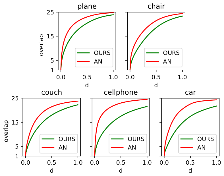
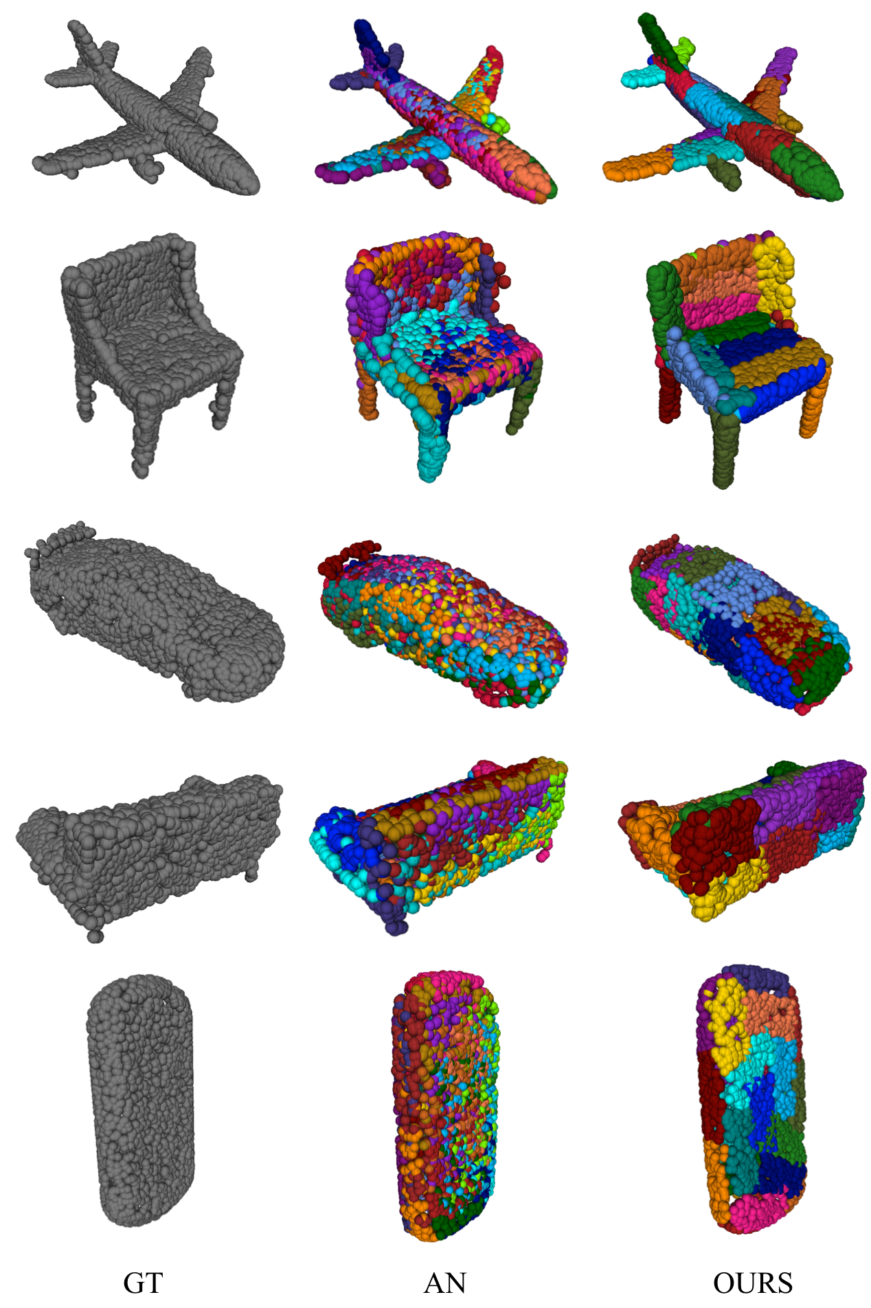
We report our results in Table 3. Note that OURS delivers comparable CHD precision while achieving significantly less overlap and higher normals accuracy as quantified by metrics $m_{\text{olap}}$ and $m_{ae}$. Fig. 7 depicts the mean overlap as a function of the neighborhood size threshold $t$ used to compute $m_{\text{olap}}^{(t)}$. Our approach consistently reduces the overlap, as illustrated by Fig. 8.

Table 3: OURS vs AN trained for PCAE. Both models were trained individually on 5 object categories from the ShapeNet dataset. While CHD is comparable for both methods, OURS delivers better normals and lower patch overlap.

obj.	method	CHD	$\mathbf{m_{ae}}$	$m_{\text{olap}}^{(0.01)}$	$m_{\text{olap}}^{(0.05)}$	$m_{\text{olap}}^{(0.1)}$	$\mathbf{m_{\text{col}}}$
plane	AN	1.07	21.26	5.90	12.08	15.39	0.006
	OURS	1.08	17.90	3.82	7.99	10.88	0.000
chair	AN	2.79	24.49	5.30	9.45	12.12	0.011
	OURS	2.82	23.06	2.85	5.78	8.09	0.000
car	AN	4.68	18.08	4.61	9.07	12.50	0.011
	OURS	3.34	17.75	2.50	4.85	7.26	0.000
couch	AN	2.10	16.83	3.74	8.07	11.67	0.000
	OURS	2.21	14.90	2.54	5.41	8.08	0.000
cellphone	AN	1.80	10.29	6.51	13.65	16.79	0.000
	OURS	1.82	9.64	2.75	6.13	8.69	0.000

SVR on TDS.

We ran two separate experiments on the T-Shirt and the Cloth. We use $4$ patches for the former as the object represents a simple rectangular shape and $14$ for the latter as the T-Shirt is more complex. We trained AN using the code provided by the authors. For both OURS and AN, we used $8000$ points randomly sampled from the GT and the same number is predicted by the networks. We trained both OURS and AN until convergence.

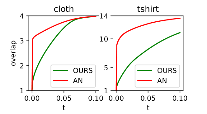
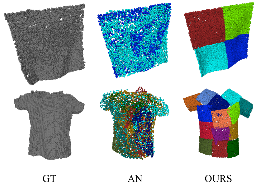
We report the results in Table 4. The results show the same trends as in the previous example, with a similar accuracy in terms of CHD but a higher normal accuracy and much less overlap for OURS. The qualitative results are depicted in Fig. 10 and the amount of overlap is quantified in Fig. 9. Note that in this case, AN suffers a number of patch collapses whereas OURS does not, which means that if the normals and curvature were needed for future processing our approach would be the better option. Besides the obvious 0D point collapses, the predictions of AN also suffer less visible but equally harmful partial collapses as demonstrated in Fig. 11.

Table 4: OURS vs AN on SVR for $\mathbf{2}$ objects from the TDS dataset. As before CHD is comparable for both methods, but OURS delivers better normals and less patch overlap.

object	method	CHD	$\mathbf{m_{ae}}$	$m_{\text{olap}}^{(0.001)}$	$m_{\text{olap}}^{(0.005)}$	$m_{\text{olap}}^{(0.05)}$	$\mathbf{m_{\text{col}}}$
cloth	AN	0.26	47.42	3.06	3.19	3.76	2
	OURS	0.28	20.06	1.37	1.75	3.53	0
tshirt	AN	0.35	42.12	8.95	10.03	12.64	7
	OURS	0.31	20.52	1.80	2.89	8.22	0

Figure 7: Patch overlap for OURS and AN trained for PCAE on the ShapeNet dataset. We plot $m_{\text{col}}^{(t)}$ as a function of $t$.

Figure 8: OURS vs AN trained for PCAE on the ShapeNet dataset. Each color denotes the points generated by one patch. Those generated by our approach are much better organized with far less overlap.

Figure 9: Patch overlap for OURS and AN trained for PCAE on the TDS dataset. We plot $m_{\text{col}}^{(t)}$ as a function of $t$.

Figure 10: OURS vs AN trained for SVR on the TDS dataset. Each color denotes the points generated by one patch. Those generated by our approach are much better organized with far less overlap and no collapsed patches.

Figure 11: Partial collapse. Even though the dark blue patch predicted by AN seems to be well developed (a), a zoomed in view reveals a partial collapse (b).

6 Conclusion

We have presented a novel and generic deep learning framework for 3D cloud point generation that makes it possible to compute analytically the differential properties of the surface the 3D points represent, without any need for post-processing. Our approach is inspired by the multi-patch approach of [16] and we have shown that we can use those differential properties during training to reduce the amount of patch overlap while delivering usable normals and curvatures, which the original approach does not do.

In future work, we will incorporate this framework in end-to-end trainable networks that require the differential properties to exploit the image information and to perform tasks such as shape-from-shading or texture mapping.

7 Supplementarty Material

We provide more details on the training and evaluation of Single-View 3D Shape Reconstruction (SVR) on the TDS dataset in Section 7.1; we perform an ablation study of the components of the deformation loss $\mathcal{L}_{\text{def}}$ in Section 7.2; and finally we analyze thoroughly the deformation properties of the predicted patches in Section 7.3.

7.1 Training and Evaluation of SVR on TDS

To evaluate the reconstruction quality of AN and OURS for SVR on the TDS dataset, some preprocessing and postprocessing steps are necessary.

The TDS dataset samples are centered around point $\mathbf{c}=\begin{bmatrix}0&0&1.1\end{bmatrix}^{\top}$, which is out of reach of the activation function tanh that AN uses in its last layer. Therefore, we translated all the data samples by $-\mathbf{c}$.

In [6], which introduced the TDS dataset, the authors align the predicted sample with its GT using Procrustes alignment [31] before evaluating the reconstruction quality. Since we do not have correspondences between the GT and predicted points, we used the Iterative Closest Point (ICP) [7] algorithm to align the two point clouds. This allows rigid body transformations only.

7.2 Deformation Loss Term Ablation Study

We have seen that the deformation loss term defined as $\mathcal{L}_{\text{def}}=\alpha_{E}\mathcal{L}_{E}+\alpha_{G}\mathcal{L}_{G}+\alpha_{\text{sk}}\mathcal{L}_{\text{sk}}+\alpha_{\text{str}}\mathcal{L}_{\text{str}}$ prevents the predicted patches from collapsing. Here we perform an ablation study of the individual components $\mathcal{L}_{E},\mathcal{L}_{G},\mathcal{L}_{\text{sk}}$ and $\mathcal{L}_{\text{str}}$ and show how each of them affects the resulting deformations that the patches undergo.

We carry out all the experiments on SVR using the cloth object from the TDS dataset and the same training/validation/testing splits as before. We employ OURS and the original loss function $\mathcal{L}=\mathcal{L}_{\text{CHD}}+\alpha_{\text{def}}\mathcal{L}_{\text{def}}+\alpha_{\text{ol}}\mathcal{L}_{\text{ol}}$ (with $\alpha_{\text{def}}=0.001$ and $\alpha_{\text{ol}}=100$, as before).

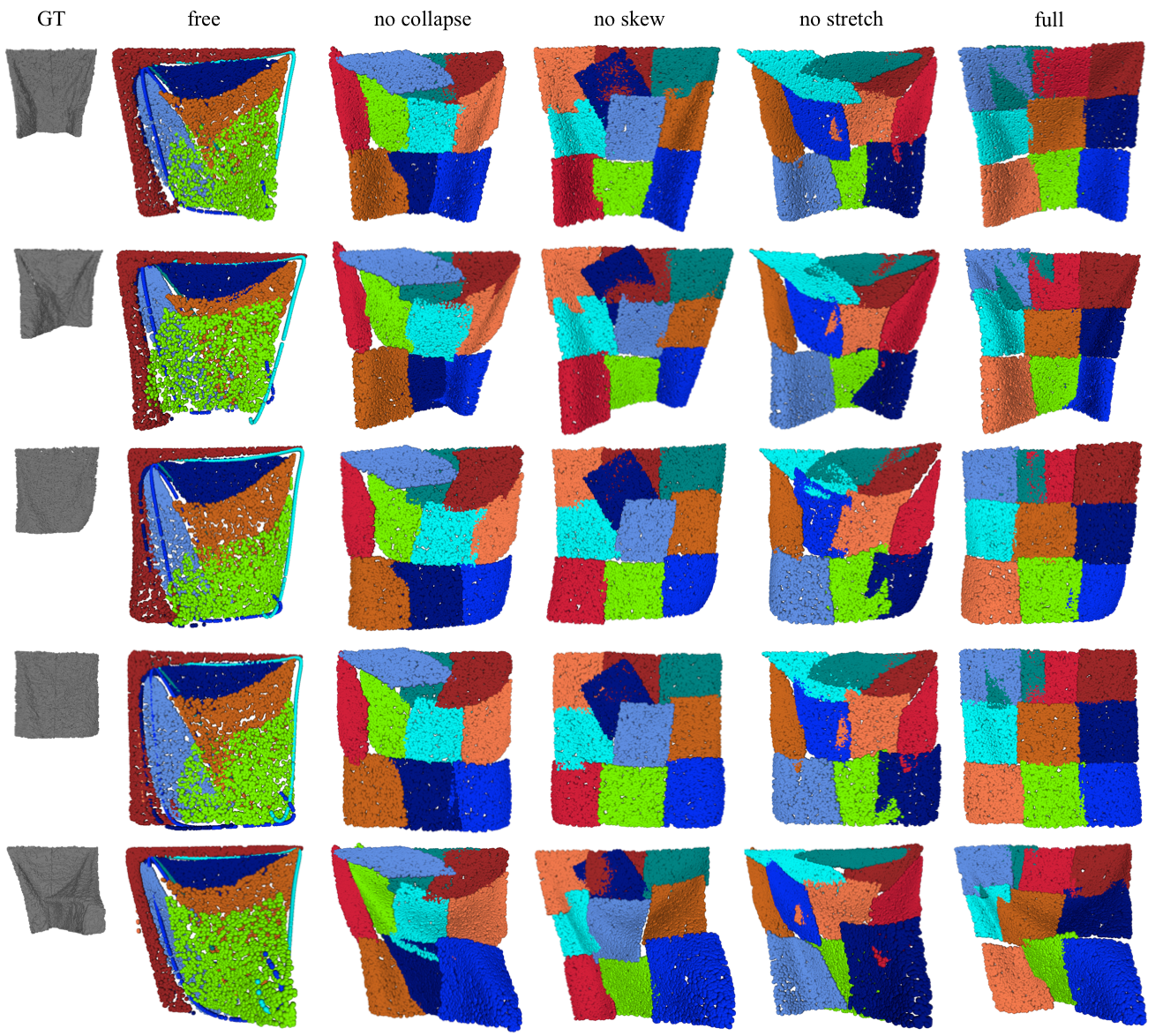
To identify the contributions of the components of $\mathcal{L}_{\text{def}}$, we switch them on or off by setting their corresponding hyperparameters $\alpha_{E},\alpha_{G},\alpha_{\text{sk}}$ and $\alpha_{\text{str}}$ to either $0$ or $1$, and for each configuration we train OURS from scratch until convergence. We list the individual configurations in Table 5.

Table 5: Configurations of the ablation study. The components of the $\mathcal{L}_{\text{def}}$ loss are either turned on or off using their corresponding hyperparameters.

Experiment	$\alpha_{E}$	$\alpha_{G}$	$\alpha_{\text{sk}}$	$\alpha_{\text{str}}$
free	0	0	0	0
no collapse	1	1	0	0
no skew	1	1	1	0
no stretch	1	1	0	1
full	1	1	1	1

Fig 12 depicts the qualitative results for all $5$ experiments on $5$ randomly selected test samples. We discuss the individual cases below:

Free:

The $\mathcal{L}_{\text{def}}$ term is completely switched off, which results in high distortion mappings and many 0D point collapses and 1D line collapses.

No collapse:

We only turn on the components $\mathcal{L}_{E}$ and $\mathcal{L}_{G}$, which by design prevent any collapse and encourage the amount of stretching along either of the axes to be uniform across the whole area of a patch. However, the patches still tend to undergo significant stretch along one axis (light red patch) and/or display a high amount of skew (light blue and light orange patch).

No skew:

Adding the $\mathcal{L}_{\text{sk}}$ component to $\mathcal{L}_{E}$ and $\mathcal{L}_{G}$ (but leaving out $\mathcal{L}_{\text{str}}$) prevents the patches from skewing, resulting in strictly orthogonal rectangular shapes. However, the patches tend to stretch along one axis (light blue and light red patch). If skew is needed to model the local geometry, the patches stay rectangular and rotate instead (dark blue patch).

No stretching:

Adding the $\mathcal{L}_{\text{str}}$ component to $\mathcal{L}_{E}$ and $\mathcal{L}_{G}$ (but leaving out $\mathcal{L}_{\text{sk}}$) results in a configuration where the patches prefer to undergo severe skew (cyan and dark green patch), but preserve their edge lengths.

All:

Using the full $\mathcal{L}_{\text{def}}$ term, with all its components turned on, results in strictly square patches with minimum skew or stretching.

Figure 12: Qualitative results of the ablation study. Each row depicts a randomly selected sample from the test set and each column corresponds to one experimental configuration. See the text for more details.

7.3 Distortion Analysis

In the previous section, we showed that the individual types of deformations that the patches may undergo—-stretching, skewing and in extreme cases collapse—-can be effectively controlled by suitable combination of the components of the loss term $\mathcal{L}_{\text{def}}$. In this section, we present a different perspective on the distortions which the patches undergo. We focus on a texture mapping task where we show that using the $\mathcal{L}_{\text{def}}$ to train a network helps learn mappings with much less distortion. Furthermore, we inspect each patch individually and analyze how the distortion distributes over its area.

7.3.1 Regularity of the Patches

We experiment on PCAE using the ShapeNet dataset, on which we train AN and OURS as in Section 5.6, i.e., using the full loss function $\mathcal{L}=\mathcal{L}_{\text{CHD}}+\alpha_{\text{def}}\mathcal{L}_{\text{def}}+\alpha_{\text{ol}}\mathcal{L}_{\text{ol}}$ with $\alpha_{\text{def}}=0.001$ and $\alpha_{\text{ol}}=100$ and with $\alpha_{E}=\alpha_{G}=\alpha_{\text{sk}}=1,\alpha_{\text{str}}=0$. Furthermore, we train one more model, OURS-strict, which is the same as OURS except that we set $\alpha_{\text{str}}=1$. In other words, OURS-strict uses the full $\mathcal{L}_{\text{def}}$ term where even stretching is penalized.

To put things in perspective, when considering the ablation study of Section 7.2, AN corresponds to the free configuration, OURS to the no skew configuration and OURS-strict to the full configuration.

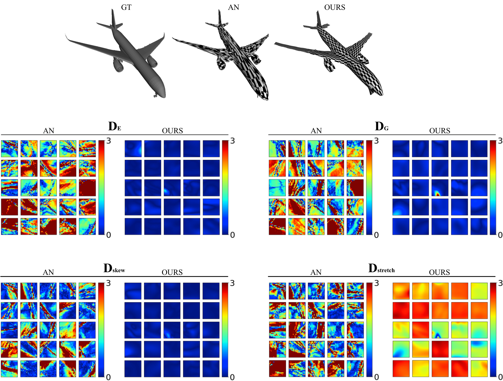
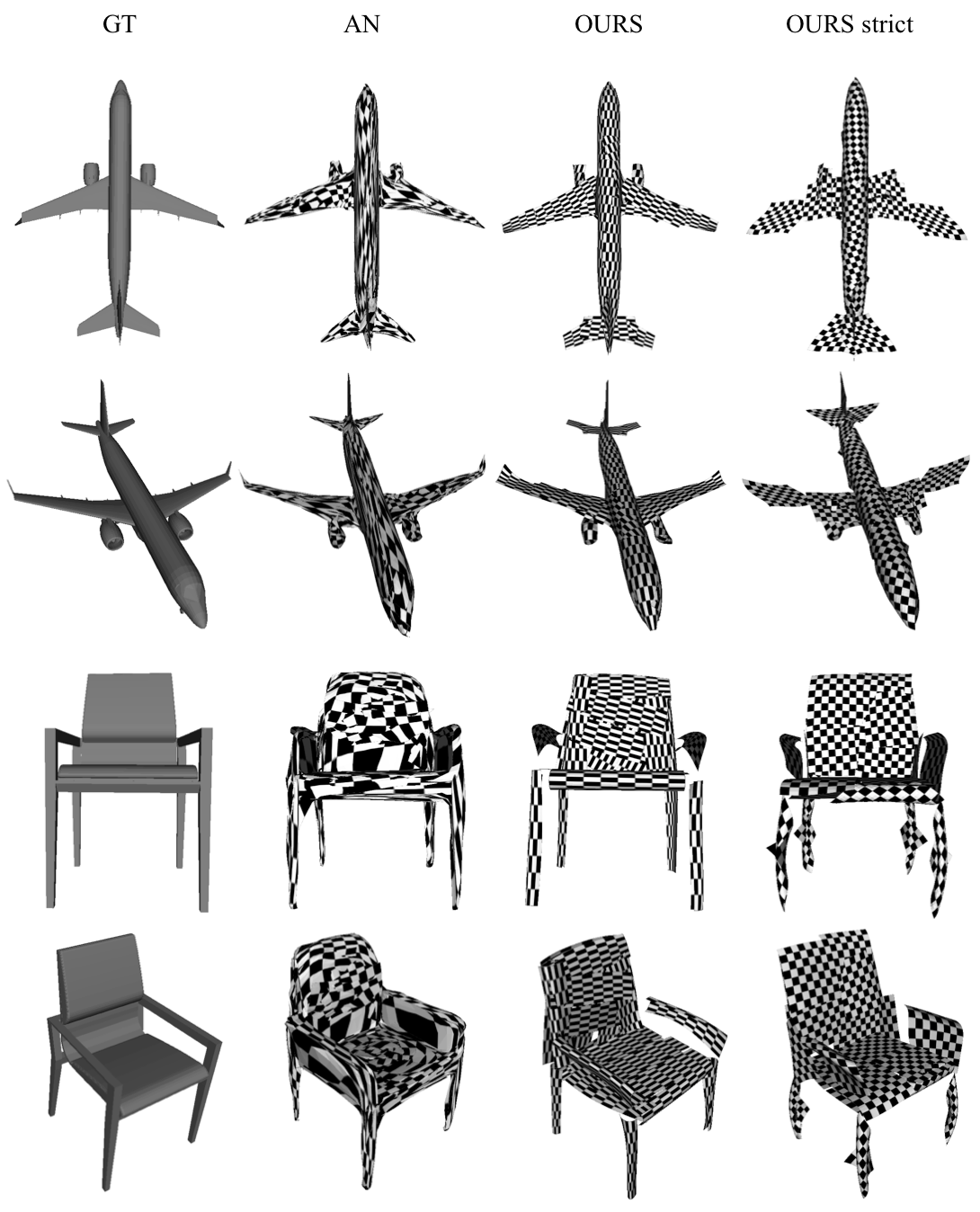
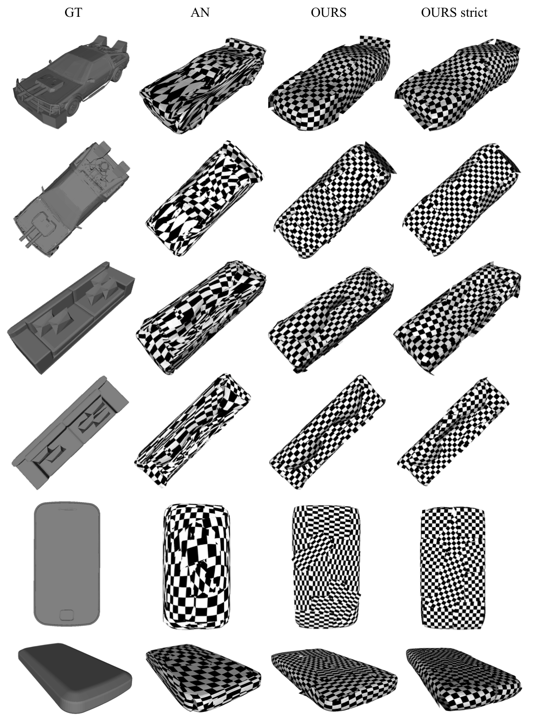
Figs. 13 and 14 depict qualitative reconstruction results for various objects from ShapeNet, where we map a regular checkerboard pattern texture to every patch. Note that while AN produces severely distorted patches, OURS introduce a truly regular pattern elongated along one axis (since stretching is not penalized) and OURS-strict delivers nearly isometric patches.

Note, however, the trade-off between the shape precision and regularity of the mapping (i.e., the amount of distortion). When considering the two extremes, AN delivers much higher precision than OURS-strict. On the other hand, OURS appears to be the best choice as it brings the best of both worlds — it delivers high precision reconstructions while maintaining very low distortion mappings.

Figure 13: Qualitative results of ShapeNet objects plane and chair reconstruction by AN, OURS and OURS-strict.

Figure 14: Qualitative results of ShapeNet objects car, couch and chair reconstruction by AN, OURS and OURS-strict.

7.3.2 Intra-patch Distortions

To obtain more detailed insights into how the patches deform, we randomly select a test data sample from the ShapeNet plane object category and analyze the individual types of deformations that each patch predicted by AN and OURS undergoes. We are interested in $4$ quantities $D_{E},D_{G},D_{\text{sk}},D_{\text{str}}$, which are proportional to the components $\mathcal{L}_{E},\mathcal{L}_{G},\mathcal{L}_{\text{sk}},\mathcal{L}_{\text{str}}$ of the deformation loss term $\mathcal{L}_{\text{def}}$.

Fig. 15 depicts the spatial distribution of the values coming from all these $4$ quantities over all $25$ patches predicted by AN and OURS. Note that while the patches predicted by AN are subject to all the deformation types and yield extremely high values, which change abruptly throughout each predicted patch, the patches predicted by OURS undergo very low distortions, which are mostly constant throughout the patches.

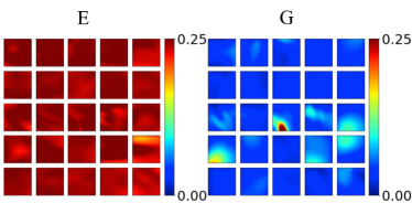
The exception is the $D_{\text{str}}$ quantity, which has high values for all the patches. This is due to the fact that OURS does not penalize stretching. This can be seen in Fig. 16, which depicts the distribution of the values of the terms $E$ and $G$ coming from the metrics tensor $g=\begin{bmatrix}E&F\\ F&G\end{bmatrix}$ across all the patches predicted by OURS. All the patches corresponding to $E$ yield high values while the ones corresponding to $G$ low values. This means that the patches prefer to stretch only along the u-axis in the 2D parametric UV space (recall that $E=\left\lVert\frac{\partial f_{\mathbf{w}}}{\partial u}\right\rVert^{2}$).

Figure 15: Spatial distribution of the quantities $D_{E},D_{G},D_{\text{sk}},D_{\text{str}}$ across all the 25 patches predicted by AN and OURS for a single test data sample from ShapeNet dataset.

Figure 16: Spatial distribution of metric tensor $g$ quantities $E$ and $G$ over all the 25 patches predicted by OURS on a single data sample from ShapeNet dataset.

References

- [1] A. Agudo, F. Moreno-Noguer, B. Calvo, and J. M. M. Montiel. Sequential Non-Rigid Structure from Motion Using Physical Priors. IEEE Transactions on Pattern Analysis and Machine Intelligence, 38(5):979–994, 2016.
- [2] H. Badino, D. Huber, Y. Park, and T. Kanade. Fast and Accurate Computation of Surface Normals from Range Images. In 2011 IEEE International Conference on Robotics and Automation, 2011.
- [3] A. Bansal, B. Russell, and A. Gupta. Marr Revisited: 2D-3D Model Alignment via Surface Normal Prediction. In Conference on Computer Vision and Pattern Recognition, 2016.
- [4] A. Bartoli, Y. Gérard, F. Chadebecq, and T. Collins. On Template-Based Reconstruction from a Single View: Analytical Solutions and Proofs of Well-Posedness for Developable, Isometric and Conformal Surfaces. In Conference on Computer Vision and Pattern Recognition, 2012.
- [5] A. Bartoli, Y. Gérard, F. Chadebecq, T. Collins, and D. Pizarro. Shape-From-Template. IEEE Transactions on Pattern Analysis and Machine Intelligence, 2015.
- [6] J. Bednarík, M. Salzmann, and P. Fua. Learning to Reconstruct Texture-Less Deformable Surfaces. In International Conference on 3D Vision, 2018.
- [7] P. Besl and N. Mckay. A Method for Registration of 3D Shapes. IEEE Transactions on Pattern Analysis and Machine Intelligence, 14(2):239–256, February 1992.
- [8] D. Bommes, B. Lévy, N. Pietroni, E. Puppo, C. Silva, M. Tarini, and D. Zorin. Quad-Mesh Generation and Processing: A Survey. Computer Graphics Forum, 32(6):51–76, September 2013.
- [9] Mario Botsch, Leif Kobbelt, Mark Pauly, Pierre Alliez, and Bruno Lévy. Polygon Mesh Processing. AK Peters / CRC Press, 2010.
- [10] A. Chang, T. Funkhouser, G. L, P. Hanrahan, Q. Huang, Z. Li, S. Savarese, M. Savva, S. Song, H. Su, J. Xiao, L. Yi, and F. Yu. Shapenet: An Information-Rich 3D Model Repository. In arXiv Preprint, 2015.
- [11] A. Dai, C. Qi, and M. Nießner. Shape Completion Using 3D-Encoder-Predictor CNNs and Shape Synthesis. In Conference on Computer Vision and Pattern Recognition, 2017.
- [12] R. Danerek, E. Dibra, C. öztireli, R. Ziegler, and M. Gross. Deepgarment : 3D Garment Shape Estimation from a Single Image. Eurographics, 2017.
- [13] T. Deprelle, T. Groueix, M. Fisher, V. G. Kim, B. C. Russell, and M. Aubry. Learning Elementary Structures for 3D Shape Generation and Matching. In Advances in Neural Information Processing Systems, 2019.
- [14] H. Fan, H. Su, and L. Guibas. A Point Set Generation Network for 3D Object Reconstruction from a Single Image. In Conference on Computer Vision and Pattern Recognition, 2017.
- [15] M. Firman, O.M. Aodha, S. Julier, and G.J. Brostow. Structured Completion of Unobserved Voxels from a Single Depth Image. In Conference on Computer Vision and Pattern Recognition, 2016.
- [16] T. Groueix, M. Fisher, V. Kim, B. Russell, and M. Aubry. Atlasnet: A Papier-Mâché Approach to Learning 3D Surface Generation. In Conference on Computer Vision and Pattern Recognition, 2018.
- [17] E. Gundogdu, V. Constantin, A. Seifoddini, M. Dang, M. Salzmann, and P. Fua. Garnet: A Two-Stream Network for Fast and Accurate 3D Cloth Draping. In International Conference on Computer Vision, 2019.
- [18] K. He, X. Zhang, S. Ren, and J. Sun. Deep Residual Learning for Image Recognition. In Conference on Computer Vision and Pattern Recognition, pages 770–778, 2016.
- [19] S. Holzer, R. B. Rusu, M. Dixon, S. Gedikli, and N. Navab. Adaptive Neighborhood Selection for Real-Time Surface Normal Estimation from Organized Point Cloud Data Using Integral Images. In International Conference on Intelligent Robots and Systems, 2012.
- [20] Alec Jacobson, Daniele Panozzo, et al. libigl: A simple C++ geometry processing library, 2018. https://libigl.github.io/.
- [21] P. Laube, M. O. Franz, and G. Umlauf. Deep Learning Parametrization for B-Spline Curve Approximation. In 3DV, 2018.
- [22] D. Ngo, J. Ostlund, and P. Fua. Template-Based Monocular 3D Shape Recovery Using Laplacian Meshes. IEEE Transactions on Pattern Analysis and Machine Intelligence, 38(1):172–187, 2016.
- [23] D. Ngo, S. Park, A. Jorstad, A. Crivellaro, C. Yoo, and P. Fua. Dense Image Registration and Deformable Surface Reconstruction in Presence of Occlusions and Minimal Texture. In International Conference on Computer Vision, 2015.
- [24] S. Parashar, D. Pizarro, and A. Bartoli. Local Deformable 3D Reconstruction with Cartan’s Connections. IEEE Transactions on Pattern Analysis and Machine Intelligence, 2019.
- [25] A. Pumarola, A. Agudo, L. Porzi, A. Sanfeliu, V. Lepetit, and F. Moreno-Noguer. Geometry-Aware Network for Non-Rigid Shape Prediction from a Single View. In Conference on Computer Vision and Pattern Recognition, June 2018.
- [26] J. Rock, T. Gupta, J. Thorsen, J. Gwak, D. Shin, and D. Hoiem. Completing 3D Object Shape from One Depth Image. In Conference on Computer Vision and Pattern Recognition, pages 2484–2493, 2015.
- [27] O. Ronneberger, P. Fischer, and T. Brox. U-Net: Convolutional Networks for Biomedical Image Segmentation. In Conference on Medical Image Computing and Computer Assisted Intervention, pages 234–241, 2015.
- [28] D. Shin, C. Fowlkes, and D. Hoiem. Pixels, Voxels, and Views: A Study of Shape Representations for Single View 3D Object Shape Prediction. In Conference on Computer Vision and Pattern Recognition, 2018.
- [29] Ayan Sinha, Asim Unmesh, Qi-Xing Huang, and Karthik Ramani. Surfnet: Generating 3d shape surfaces using deep residual networks. Conference on Computer Vision and Pattern Recognition, 2017.
- [30] A.A. Soltani, H. Huang, J. Wu, T. D. Kulkarni, and J.B. Tenenbaum. Synthesizing 3D Shapes via Modeling Multi-View Depth Maps and Silhouettes with Deep Generative Networks. In Conference on Computer Vision and Pattern Recognition, pages 2511–2519, 2017.
- [31] Mikkel B. Stegmann and David Delgado Gomez. A Brief Introduction to Statistical Shape Analysis. Technical report, University of Denmark, DTU, 2002.
- [32] Francis Williams, Teseo Schneider, Claudio T. Silva, Denis Zorin, Joan Bruna, and Daniele Panozzo. Deep geometric prior for surface reconstruction. Conference on Computer Vision and Pattern Recognition, 2019.
- [33] J. Wu, Y. Wang, T. Xue, X. Sun, W.T. Freeman, and J.B. Tenenbaum. MarrNet: 3D Shape Reconstruction via 2.5D Sketches. In Advances in Neural Information Processing Systems, 2017.
- [34] Y. Yang, C. Feng, Y. Shen, and D. Tian. FoldingNet: Point Cloud Auto-Encoder via Deep Grid Deformation. In Conference on Computer Vision and Pattern Recognition, June 2018.