Mechanism of Universal Conductance Fluctuations

Universal conductance fluctuations [1,2] are usually observed in the form of aperiodic oscillations in the magnetoresistance of thin wires as a function of the magnetic field $B$ [3] (Fig. 1). According to the theory [1,2], the conductance $G(B)$ at a given magnetic field $B$ undergoes fluctuations of the order of $e^{2}/h$ under the variation of the impurity configuration; fluctuations in $G(B)$ and $G(B+\Delta B)$ are statistically independent if $\Delta B$ exceeds a certain characteristic scale $\xi_{B}$. It is reasonable to expect that oscillations in $G(B)$ are completely random at scales exceeding $\xi_{B}$. Then, their Fourier analysis should reveal a white noise spectrum (i.e., frequency-independent plateau) at frequencies below $\xi_{B}^{-1}$.

Comparison with the results for 1D systems [4] suggests another scenario. A magnetic field perpendicular to a thin wire creates a quadratic potential along this wire [5], which effectively restricts the length of the system $L$; hence, the variation of the magnetic field is similar to the variation of $L$. The resistance $\rho$ of a one-dimensional system is a strongly fluctuating quantity and the form of its distribution function $P(\rho)$ strongly depends on first several moments. Indeed, the Fourier transform of $P(\rho)$ specifies the characteristic function

$${F}(t)=\left\langle e^{i\rho t}\right\rangle=\sum_{n=0}^{\infty}\frac{(it)^{n}}{n!}\left\langle\rho^{n}\right\rangle\,,$$

which is the generating function of the moments $\left\langle\rho^{n}\right\rangle$. If all moments of the distribution are known, the function ${F}(t)$ can be constructed using them, and the function $P(\rho)$ is then determined by the inverse Fourier transform. If an increase in the moments $\left\langle\rho^{n}\right\rangle$ with $n$ is not too fast, the contributions of higher moments are suppressed by a factor of $1/n!$, whereas first several moments are significant. These moments are oscillating functions of $L$,

$$\left\langle\rho\right\rangle=a_{1}(L)+b_{1}(L)\cos(\omega_{1}L+\varphi_{1}),$$

$$\left\langle\rho^{2}\right\rangle=a_{2}(L)+b_{2}(L)\cos(\omega_{2}L+\varphi_{2})+$$

$$+b_{3}(L)\cos(\omega_{3}L+\varphi_{3})\,,\quad\mbox{etc.,}$$

where $a_{k}(L)$ and $b_{k}(L)$ are monotonic functions. The reason is that the growth exponent for $\left\langle\rho^{n}\right\rangle$ is determined by the $(2n\!+\!1)$th order algebraic equation (see Appendix), one of whose root is always real, whereas the other roots are complex for energies in the allowed band. Consequently, there are $n$ pairs of complex conjugate roots, which ensure the presence of $n$ frequencies in oscillations of $\left\langle\rho^{n}\right\rangle$. The frequencies $\omega_{k}$ are usually incommensurate, but their incommensurability vanishes in the deep of the allowed band at weak disorder. According to this picture, oscillations in $G(B)$ shown in Fig. 1 are determined by the superposition of incommensurate harmonics and their Fourier spectrum should contain discrete frequencies. This picture is indirectly confirmed by the experimental data obtained in [6] and cited in [4], according to which the distribution function $P(\rho)$ is not stationary, but demonstrates systematic aperiodic variations.

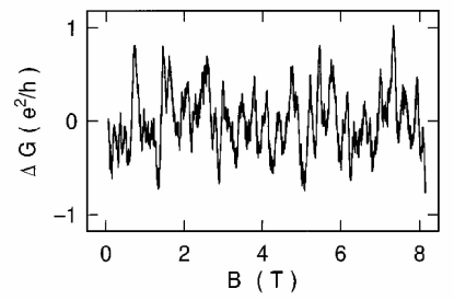
Figure 1: Magnetic field dependence of the conductance of the thin Au wire [3].

It is clear from the above that the Fourier analysis of the function $G(B)$ makes it possible to establish which of two scenarios is true. However, the dependence $G(B)$ shown in Fig. 1 cannot be used directly because a sharp cutoff of experimental data results in the appearance of slowly decaying oscillations in its Fourier transform and chaotization of the spectrum . To obtain explicit results, it is necessary to use an appropriate smoothing function.

Let the function $f(x)$ be the superposition of discrete harmonics and be real. Then,

$$f(x)=\sum_{k}A_{k}{\rm e}^{i\omega_{k}x}=\frac{1}{2}\sum_{k}\left[A_{k}{\rm e}^{i\omega_{k}x}+A_{k}^{*}{\rm e}^{-i\omega_{k}x}\right]\,,$$

where the frequencies $\omega_{k}$ can be considered as positive without loss of generality. Then, the Fourier transform of $f(x)$ has the form

$$F(\omega)=\pi\sum_{k}\left[A_{k}\delta(\omega+\omega_{k})+A_{k}^{*}\delta(\omega-\omega_{k})\right]\,,$$

and its modulus

$$|F(\omega)|=\pi\sum_{k}|A_{k}|\left[\delta(\omega+\omega_{k})+\delta(\omega-\omega_{k})\right]$$

depends only on the intensities of spectral lines and does not contain information on phase shifts in the corresponding harmonics. Since $|F(\omega)|$ is an even function, it is possible to consider only positive $\omega$ values and to omit the first delta function in Eq. (5).

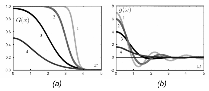
Figure 2: (a) Function $G(x)$ given by Eq. (9) and (b) its Fourier transform $g(\omega)$ at (1) $\mu=3.5$, $T=0.125$; (2) $\mu=3$, $T=0.25$; ( 3) $\mu=2$, $T=0.5$; and ( 4) $\mu=T\ln 2$, $T=0.8$.

Since the function $f(x)$ can be experimentally measured only in a certain finite $x$ range, we in practice have

$$f(x)=\frac{1}{2}\sum_{k}\left[A_{k}{\rm e}^{i\omega_{k}x}+A_{k}^{*}{\rm e}^{-i\omega_{k}x}\right]G(x)\,,$$

where the function $G(x)$ is unity within the working range and zero beyond it; further, it will be smoothed. Then, instead of Eq. (4), we obtain

$$F(\omega)=\frac{1}{2}\sum_{k}\left[A_{k}g(\omega+\omega_{k})+A_{k}^{*}g(\omega-\omega_{k})\right]\,,$$

where $g(\omega)$ is the Fourier transform of $G(x)$, which is real for even function $G(x)$. Thus, the restriction of the working range leads to the replacement of delta functions by spectral lines with finite widths. If discrete frequencies are well separated and the function $g(\omega)$ is strongly localized near zero, one can neglect the overlapping of functions $g(\omega\pm\omega_{k})$ and write at positive frequencies

$$|F(\omega)|^{2}\approx\frac{1}{4}\sum_{k}|A_{k}|^{2}g^{2}(\omega-\omega_{k})\,.$$

It is preferable to use the function $|F(\omega)|^{2}$ (so-called power spectral density [7]) because the integral of this function over all frequencies is equal to the integral of $f^{2}(x)$ over all $x$ values. Consequently, change in the spectrum of $f(x)$ at fixed rms fluctuations results in the redistribution of intensities between different frequencies at the conservation of the total spectral power.

It is easy to see that, to obtain a clear picture in the case of a discrete spectrum, it is necessary to have a possibly narrower shape of spectral lines determined by $g(\omega)$, which can be achieved by the appropriate choice of the function $G(x)$. The general strategy is determined by the properties of integrals of rapidly oscillating functions [8]. If the function $f(x)$ has discontinuity, its Fourier transform decreases at high frequencies as $1/\omega$; if the $n$th derivative is discontinuous, then $F(\omega)\sim\omega^{-n-1}$. The Fourier transform of a smooth function $f(x)$ is calculated by shifting the contour of integration to a complex plane and is determined by the nearest singularity or saddle point, which leads to the dependence $F(\omega)\sim\exp(-\alpha\omega)$. If the regular function is obtained by means of a weak smoothing of a singularity, the $\alpha$ value is small and the exponential is manifested only at very high frequencies, whereas the behavior corresponding to the singularity holds in the remaining region. In our case, it is necessary to smooth the discontinuity of $G(x)$. It should be clear that weak smoothing is inefficient, while strong smoothing leads to small values of $G(x)$ near the boundaries of the working range and to loss of experimental information; so, a reasonable compromise is required.

Let $G(x)$ be the $x$-symmetrized Fermi function

$$G(x)=\frac{1}{1+{\rm e}^{(x-\mu)/T}+{\rm e}^{(-x-\mu)/T}}=$$

$$=\frac{1}{1+2{\rm e}^{-\mu/T}{\rm cosh}(x/T)}\,,$$

whose Fourier transform is given by the integral

$$g(\omega)=\int\limits_{-\infty}^{\infty}\frac{{\rm e}^{i\omega x}\,dx}{b\,{\rm cosh}\beta x+c}=\frac{2\pi}{b\beta{\rm sinh}x_{0}}\frac{\sin(\omega x_{0}/\beta)}{{\rm sinh}(\omega\pi/\beta)}\,,$$

$$\qquad x_{0}={\rm arccosh}(c/b)\,.$$

If $x=B-\mu_{0}$ is chosen in our case, experimental data correspond to the interval $|x|\leq\mu_{0}$ with $\mu_{0}=4$ (in units of tesla). We accepted $\mu=\mu_{0}-4T$, which ensures the small value $G(\mu_{0})\approx 0.02$ at boundaries of the interval. As clear from Fig. 2, the behavior $g(\omega)=2\sin{\mu\omega}/\omega$ characteristic of the sharp cutoff prevails at small $T$ values (lines 1 and 2). It seems reasonable to choose $\mu=2$ and $T=0.5$ (line 3); in this case, 50% of experimental data are effectively used, while the lineshape is approximately the same as in the case of $\mu=T\ln{2}$, where $x_{0}=0$, $g(\omega)=2\pi T^{2}\omega/{\rm sinh}{\pi T\omega}$ and oscillations disappear completely (line 4).

The results of processing experimental data (Fig. 1) with the indicated smoothing function are shown in Fig. 3. The spectrum obviously consists of discrete lines, which confirms the second scenario given in beginning . However, the spectrum in the range $\omega\mathbin{\lower 3.0pt\hbox{$\hbox to0.0pt{\raise 5.0pt\hbox{$\char 60\relax$}\hss}\mathchar 29208\relax$}}2\pi/\xi_{B}$ (where $\xi_{B}$ was estimated as the average distance between neighboring maxima or minima in Fig. 1)  is similar to discrete white noise: in a rough approximation, the lines are equidistant and their intensities are more or less the same. Since the sum over frequencies is often approximated by an integral, discrete white noise does not differ in many properties from continuous white noise. Let, for example,

$$F(\omega)=\pi\sum_{k}\left[A_{k}\delta(\omega+\omega_{k})+A_{k}^{*}\delta(\omega-\omega_{k})\right]H(\omega)\,,$$

where the frequencies $\omega_{k}$ are equidistant ($\omega_{k+1}-\omega_{k}=\Delta$), the amplitudes $A_{k}$ are the same in modulus ($|A_{k}|=A$) and have completely random phases, while $H(\omega)$ is an even function restricting the spectrum to the range $|\omega|\mathbin{\lower 3.0pt\hbox{$\hbox to0.0pt{\raise 5.0pt\hbox{$\char 60\relax$}\hss}\mathchar 29208\relax$}}\Omega$. Then, determining $f(x)$ by means of the inverse Fourier transform, we obtain the correlation function

$$\langle f(x)f(x^{\prime})\rangle=\frac{1}{2}\sum_{k}A^{2}H^{2}(\omega_{k}){\rm e}^{i\omega_{k}(x-x^{\prime})}\approx$$

$$\approx\frac{1}{2}A^{2}\Delta h(x-x^{\prime})\,,$$

where $h(x)$ is the Fourier transform of $H^{2}(\omega)$. If the function $H(\omega)$ is smooth, $h(x)$ decreases exponentially at a scale of $\Omega^{-1}$ in agreement with the diagrammatic results obtained in [1,2].

In conclusion, the results obtained in this work reconcile two alternative scenarios described at the beginning. On the one hand, the spectrum is discrete, confirming the second scenario, where aperiodic conductance oscillations are due to the superposition of incommensurate harmonics. On the other hand, the spectrum as a whole resembles discrete white noise, which is close in properties to continuous white noise. Universal conductance fluctuations are observed in a lot of works (see [9, 10] and references therein), and it would be interesting to process the corresponding experimental data in the spirit of the present paper.

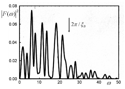
Figure 3: Fourier analysis of the experimental data shown in Fig. 1 with the smoothing function (9) at $\mu=2$, $T=0.5$.

Appendix. Derivation of Eq. (2)

Let us consider the one-dimensional Anderson model specified by the discrete Schr$\ddot{o}$dinger equation

$$\Psi_{n+1}+\Psi_{n-1}+V_{n}\Psi_{n}=E\Psi_{n}\,,$$

where $E$ is the energy measured from the center of the band, $V_{n}$ are independent random variables with zero mean and variance $W^{2}$, while the hopping integral is taken to be unity. Rewriting Eq. $(A.1)$ in the form

$$\left(\begin{array}[]{cc}\!\!\Psi_{n+1}\!\!\\ \!\!\Psi_{n}\!\!\end{array}\right)\,=\left(\begin{array}[]{cc}\!E-V_{n}&-1\!\\ \!1&0\!\end{array}\right)\,\left(\begin{array}[]{cc}\!\!\Psi_{n}\!\!\\ \!\!\Psi_{n-1}\!\!\end{array}\right)\,,$$

and performing $n$ iterations, one can easily obtain

$$\left(\begin{array}[]{cc}\Psi_{n+1}\\ \Psi_{n}\end{array}\right)\,=\left(\begin{array}[]{cc}\tau_{11}&\tau_{12}\\ \tau_{21}&\tau_{22}\end{array}\right)\,\left(\begin{array}[]{cc}\Psi_{1}\\ \Psi_{0}\end{array}\right)\,.$$

Here, the matrix ${\tau}=||\tau_{ij}||$ is the product of $n$ matrices of the form $(A.2)$ and satisfies an obvious recurrence relation, which can be represented in terms of matrix elements,

$$y_{n+1}=(E-V_{n})y_{n}+z_{n}\,,\qquad z_{n+1}=-y_{n}\,,$$

where $y_{n}=\tau^{(n-1)}_{12}$, $z_{n}=\tau^{(n-1)}_{11}$ or $y_{n}=\tau^{(n-1)}_{22}$, $z_{n}=\tau^{(n-1)}_{21}$. It is substantial that $y^{(n-1)}$ and $z^{(n-1)}$ do not contain the quantity $V_{n}$ and can be averaged independently of it. Setting $w^{(1)}_{n}=\langle y_{n}^{2}\rangle$, $w^{(2)}_{n}=\langle y_{n}z_{n}\rangle$, $w^{(3)}_{n}=\langle z_{n}^{2}\rangle$ for the second moments, one can easily come to the equation

$$\left(\begin{array}[]{ccc}w^{(1)}_{n+1}\\ w^{(2)}_{n+1}\\ w^{(3)}_{n+1}\end{array}\right)\,=\left(\begin{array}[]{ccc}E^{2}+W^{2}&2E&\,\,\,1\\ -E&-1&\,\,\,0\\ 1&0&\,\,\,0\end{array}\right)\,\left(\begin{array}[]{ccc}w^{(1)}_{n}\\ w^{(2)}_{n}\\ w^{(3)}_{n}\end{array}\right)\,,$$

Its solution is exponential, $w^{(i)}_{n}\sim\lambda^{n}$, where $\lambda$ is an eigenvalue of the matrix. Setting $\lambda=1+x$, it is easy to obtain an equation for $x$, which has the following form in the limit of the continuous Schr$\ddot{o}$dinger equation:

$$x\left(x^{2}+4{\cal E}\right)=2W^{2}$$

where $\cal E$ is the energy measured from the band edge. The equation for the growth exponent of the fourth moments can be obtained similarly:

$$x\left(x^{2}+{4\cal E}\right)\left(x^{2}+16{\cal E}\right)=42W^{2}x^{2}+96W^{2}{\cal E}\,.$$

The structure of equations for arbitrary $2n$th moments can be established using argumentation presented in Section 4 in [4], where a slightly different formalism was used. Deep in the allowed and forbidden bands, only diagonal elements can be retained in matrices (43) and (47) in [4] and their analogs for higher moments. As a result, we arrive at the equation

$$\prod_{k=0}^{2n}\left[x+(n\!-\!k)\delta-B_{n}^{k}\epsilon^{2}\right]=O(\epsilon^{4})\,,$$

where $\epsilon^{2}=W^{2}/4{\cal E}$, $\delta^{2}=-{\cal E}$, $B_{n}^{k}=n(2n\!-\!1)+3k(k\!-\!2n)$. A similar equation near the band edge

$$x^{2n+1}=\sum\limits_{k=0}^{k_{max}}C_{k}W^{2k}x^{2n+1-3k}\,,\quad k_{max}=\left[\frac{2n+1}{3}\right]$$

follows from observation that all terms of the equation have the same order of magnitude at $x\sim\delta\sim\epsilon^{2}$ and only combinations $\delta^{2n}\epsilon^{2m}$ with $n\geq m$ are allowed, among which only $\delta^{2n}\epsilon^{2n}\sim W^{2n}$ remain finite at $\delta\to 0$.

Landauer resistance $\rho$ is determined by a quadratic form of the matrix elements $\tau_{ij}$ [4]. Consequently, growth exponents for $\langle\rho^{n}\rangle$ coincide with those for the $2n$th moments of $\tau_{ij}$. An expression for $\langle\rho^{n}\rangle$ contains a linear combination of the corresponding exponents, which leads to Eq. (2) if the complex-valued exponents are taken into account.

References

- [1] P. A. Lee, A. D. Stone, Phys. Rev. Lett. 55, 1622 (1985); P. A. Lee, A. D. Stone, H.Fukuyama, Phys. Rev. B 35, 1039 (1987).
- [2] B. L. Altshuler, JETP Lett. 41, 648 (1985); B. L. Altshuler, D. E. Khmelnitskii, JETP Lett. 42, 359 (1985).
- [3] S. Washburn, R. A. Webb, Adv. Phys. 35, 375 (1986).
- [4] I. M. Suslov, J. Exp. Theor. Phys. 129, 877 (2019).
- [5] L. D. Landau, E. M. Lifshitz, Quantum Mechanics, Pergamon, 1977.
- [6] D. Mailly, M. Sanquer, J. Phys. (France) I 2, 357 (1992).
- [7] W. H. Press, B. P. Flannery, S. A. Teukolsky, W. T. Wetterling, Numerical Recipes in Fortran, Cambridge University Press, 1992.
- [8] A. B. Migdal, Qualitative Methods in Quantum Theory, Nauka, Moscow, 1975.
- [9] M. A. Aamir, et al, Phys. Rev. Lett. 121(13), 136806 (2018).
- [10] S. Islam, et al, Phys. Rev. B 97, 241412R (2018).
- [11]