Gravitational waveforms of binary neutron star inspirals using post-Newtonian tidal splicing

Abstract

The tidal deformations of neutron stars within an inspiraling compact binary alter the orbital dynamics, imprinting a signature on the gravitational wave signal. Modeling this signal could be done with numerical-relativity simulations, but these are too computationally expensive for many applications. Analytic post-Newtonian treatments are limited by unknown higher-order nontidal terms. This paper further builds upon the “tidal splicing” model in which post-Newtonian tidal terms are “spliced” onto numerical relativity simulations of black-hole binaries. We improve on previous treatments of tidal splicing by including spherical harmonic modes beyond the (2,2) mode, expanding the post-Newtonian expressions for tidal effects to 2.5 order, including dynamical tide corrections, and adding a partial treatment of the spin-tidal dynamics. Furthermore, instead of numerical relativity simulations, we use the spin-aligned binary black hole (BBH) surrogate model “NRHybSur3dq8” to provide the BBH waveforms that are input into the tidal slicing procedure. This allows us to construct spin-aligned, inspiraling TaylorT2 and TaylorT4 splicing waveform models that can be evaluated quickly. These models are tested against existing binary neutron star and black hole–neutron star simulations. We implement the TaylorT2 splicing model as an extension to “NRHybSur3dq8,” creating a model that we call “NRHybSur3dq8Tidal.”

I Introduction

In August 2017, the network of interferometers consisting of Advanced LIGO Aasi et al. (2015) and VIRGO Acernese et al. (2015) first observed the gravitational radiation from the inspiral and merger of a binary neutron star (BNS) Abbott et al. (2017), opening the door to exploring extremely compact objects other than binary black holes (BBH). Coincident detection with the electromagnetic observational counterpart GRB 170817A Abbott et al. (2017), showed that these systems are the progenitors of short gamma-ray bursts, and herald the start of multimessenger astronomy. Additionally, this detection served as a probe of the neutron star equation of state (EOS) Abbott et al. (2017); Radice et al. (2018), and provided constraints on the gravitational wave speed Abbott et al. (2017). As the detectors’ sensitivities improve, observing more such systems will further constrain the governing physics Del Pozzo et al. (2013); Kumar et al. (2017). However, capturing all of the information encoded in the measured signals requires detailed, accurate templates that precisely describe waveforms from BNS or black hole–neutron star (BHNS) systems.

A common approach to generate BHNS and BNS waveforms is to create analytic and phenomenological models that capture the behavior of BHNS and BNS systems, often in the form of additional corrections to BBH waveform models. Within the post-Newtonian (PN) formalism, Ref Vines et al. (2011) first computed the leading-order tidal effects on the orbital evolution, characterized by the static quadrupolar tidal deformability, $\bar{\lambda}_{2}$. However, recent work suggests that the choice of the BBH model used as the background for tidal corrections can impact parameter estimation Chakravarti et al. (2019); Samajdar and Dietrich (2018), suggesting that errors in PN waveforms for BNS and BHNS systems might be dominated by unknown higher-order vacuum terms rather than tidal terms. Within the frequency domain, work has gone into mitigating biases caused by this problem through partially expanding the nonspinning point-mass equations to higher-orders Messina et al. (2019).

An alternative to the PN formalism is to implement tidal corrections as an extension to the effective one-body (EOB) formalism Damour and Nagar (2010). Current tidal EOB models include the time domain model SEOBNRv4T Hinderer et al. (2016); Steinhoff et al. (2016), whereby the calibrated EOB model SEOBNRv4 Bohé et al. (2017) is extended by including additional static higher-order effects Bini et al. (2012); Baiotti et al. (2011); Steinhoff et al. (2016); Dietrich and Hinderer (2017). Another distinct EOB model, TEOBResumS Nagar et al. (2018, 2019), also includes spin aligned as well as self-spin effects through next-to-next-to leading order, and a postmerger description informed by black-hole perturbation theory and NR BBH waveforms.

Additional models have been constructed by calibrating to numerical simulations of BNS and BHNS binaries. The LEA+ model Kumar et al. (2017) is a frequency domain waveform model calibrated to a series of BHNS simulations with mass ratios of $q>2$ Lackey et al. (2014) as an enhancement to the SEOBNRv2 model Taracchini et al. (2014). While LEA+ is a full waveform model, it is valid only over the limited parameter space of the simulations used to calibrate it, i.e., $q>2$.

The frequency domain models SEOBNRv4_ROM_NRTidal, PhenomD_NRTidal, and PhenomPv2_NRTidal Dietrich et al. (2019a) are built by combining the BBH models SEOBNRv4_ROM Bohé et al. (2017), PhenomD Husa et al. (2016); Khan et al. (2016), and PhenomPv2 Schmidt et al. (2012, 2015) with the NRTidal model Dietrich et al. (2017). NRTidal is a phenomenological fit of BNS/BHNS simulation data to PN-like coefficients. While these models cover a wide range of BNS parameter space, the fits are calibrated to a limited number of waveforms and seem to overestimate the tidal effects during the inspiral Dietrich et al. (2019a), though improvements to these models are expected to eliminate this problem Dietrich et al. (2019b).

The most accurate means of obtaining BNS and BHNS waveform templates would be to run full numerical simulations. Running simulations that incorporate the relevant matter physics for BHNS/BNS is a field of active development Foucart et al. (2013); Lackey et al. (2014); Lovelace et al. (2013); Kawaguchi et al. (2015); Haas et al. (2016); Hinderer et al. (2016); Dietrich et al. (2017, 2018); Foucart et al. (2019); Kiuchi et al. (2020). However, the range of possible systems spans not just the masses and spins of the components, but also includes all allowable EOSs. This would require a large number of simulations to populate such a high dimensional parameter space. Furthermore, the large computational cost of such simulations makes them impractical for parameter estimation purposes.

On the other hand, numerical simulations of BBH systems have made great strides over recent years, and there are now public repositories of hundreds of simulations for binaries with a variety of different initial masses and spins Aylott et al. (2009); Ajith et al. (2012); Hinder et al. (2014); Mroué et al. (2013); Jani et al. (2016); Healy et al. (2017, 2019); Huerta et al. (2019); Boyle et al. (2019). Furthermore, surrogate models now allow interpolation of numerical-relativity waveforms to desired values of initial masses and spins Field et al. (2014); Pürrer (2014); Blackman et al. (2015, 2017a, 2017b); Varma et al. (2019a, b). Reference Varma et al. (2019a) showed that surrogate models can robustly generate faithful representations of binary black hole systems with spin magnitudes $\chi<0.8$ and masses low enough to be valid for BNS systems ($M\geq 2.25M_{\odot}$).

We build on a hybrid method called “tidal splicing” Barkett et al. (2016), which computes inspiral waveforms for BNS and BHNS by combining the accuracy of numerical BBH simulations with the efficiency of PN models for tidally deformable systems. This method does so by decomposing the numerical BBH waveform in a manner akin to the PN formalism and using this decomposition to replace all orders of the vacuum terms in the analytic PN expansion with their numerical equivalents. We combine these vacuum terms with the analytic tidal PN terms to build up a waveform that models the inspiral of a BNS/BHNS.

In this paper, we continue the development of tidal splicing beyond Ref. Barkett et al. (2016) by extending the method to spinning systems and spherical harmonic modes beyond the (2,2) mode. Using results from newly available EOB models that incorporate higher PN effects Bini et al. (2012); Baiotti et al. (2011); Steinhoff et al. (2016); Dietrich and Hinderer (2017), we also extend the known higher-order tidal effects from EOB to the time domain PN approximants. Previous explorations of tidal splicing Barkett et al. (2016) were based on particular individual numerical relativity BBH simulations, and therefore could be tested only for the masses and spins of those simulations. Here, instead of using numerical relativity simulations directly, we will use the hybridized surrogate model ‘NRHybSur3dq8’ Varma et al. (2019a) as our BBH base.

We organize this paper as follows: in Sec II we summarize the current existing work on time domain tidal waveforms in the PN framework; in Sec III we discuss how we partially extend the PN tidal approximants to 2.5PN order and how we correct the dynamical tide effects for spinning NS; in Sec IV we explain our method of tidal splicing; and in Sec V we compare tidal splicing with some recent BHNS and BNS simulations.

Except where otherwise noted, we shall use the subscripts $A,B$ to refer to the individual NS or BH objects, the subscripts $\ell=2,3,\ldots$ refer usually to the specific polar mode of the tidal effect in consideration (i.e., 2=quadrupolar, 3=octopolar,…), while the $\ell,m$ superscripts will typically correspond to the spin-weighted spherical harmonic modes ${}_{-2}Y^{\ell m}$ of the waveform. We chose units of $G=c=1$.

II Post-Newtonian Theory

The PN approximation describes the binary’s orbital behavior as series expansions that are valid in the slow-moving, weak-field regime. The expansion parameter is the characteristic velocity of the inspiraling objects, $v$ (another common parameter is $x=v^{2}$). We denote an expansion term of order $\mathcal{O}(v^{n})$ by the label $\frac{n}{2}$PN (e.g. 2.5PN corresponds to $v^{5}$ beyond leading order). A more detailed summary of PN theory as it pertains to point-particle systems can be found in Blanchet (2014).

We start with a quasicircular binary system of a pair of compact objects with component masses $m_{A}$ and $m_{B}$, with total mass $M$, and spins of dimensionless magnitude $\chi_{A}$ and $\chi_{B}$ aligned with the orbital angular momentum. Here $\chi_{A}=S_{A}/m_{A}^{2}$, where $S_{A}$ is the spin angular momentum. We define the mass ratio $q$ as the larger mass over the smaller mass, $m_{A}/m_{B}$, so that $q\geq 1$. For convenience, we also define the mass fraction $X_{A}=m_{A}/M$, and symmetric mass ratio $\nu=X_{A}X_{B}$.

When the objects are not simply point particles, but extended objects like neutron stars, each object responds to the changing tidal fields. The leading tidal effects are the result of the deformation of the NS due to the tidal field generated by the other object in the binary. This effect is characterized by the dimensionless $\ell$-polar tidal deformability parameter, $\bar{\lambda}_{\ell}$. Other commonly used parameters are dimensionful tidal parameter $\lambda_{\ell}$ or the tidal love number $k_{\ell}$, and are related to $\bar{\lambda}_{\ell}$ by the NS radius $R_{A}$ or compactness $C_{A}=m_{A}/R_{A}$ according to

$$\bar{\lambda}_{\ell A}= \frac{2}{(2\ell-1)!!}\frac{k_{\ell A}}{C_{A}^{2\ell+1}}=\frac{\lambda_{\ell A}}{m_{A}^{2\ell+1}}.$$ (1)

As each object in the binary can have its own deformability, we add the subscript $A,B$ to specify the particular object.

In the following, we will often separate the PN expressions into two parts: “BBH terms,” the terms that describe a BBH inspiral, and “tidal terms,” the terms that describe corrections due to one or more of the objects being something other than a BH. This will be important for tidal splicing, for which we replace the BBH terms with numerical relativity (or a surrogate model thereof) but we use the PN expressions for the tidal terms. The tidal deformability $\bar{\lambda}_{\text{BH}}$ of black holes is generally treated as vanishing but is somewhat difficult to define Fang and Lovelace (2005); here we will set $\bar{\lambda}_{\text{BH}}=0$, so all terms that depend on $\bar{\lambda}_{\ell}$ are tidal terms. The BBH terms are identical to point-particle terms up to 4PN for nonspinning BHs and 2.5PN (with the exception of 2PN quadrupole moment terms) for spinning BHs Alvi (2001). We include the 2PN correction for spinning BHs in Sec. III.1.

II.1 Orbital evolution

Two equations govern the evolution of the quasicircular binary system in PN theory. The first relates the orbital phase $\phi$ to $v$ by a correspondence with the orbital frequency, $\omega$,

$$\omega=\frac{d\phi}{dt}=\frac{v^{3}}{M}.$$ (2)

The other equation is the energy balance equation as the emission of gravitational radiation drives the adiabatic evolution by bleeding away the orbital energy, $E(v)$. If the energy flux is given by $F(v)$, then this energy balance equation is

$$\frac{dE(v)}{dt}=-F(v).$$ (3)

The quadrupolar tidal deformability $\bar{\lambda}_{2}$ enters $E(v)$ and $F(v)$ first at 0PN as a $\mathcal{O}(v^{10})$ term , and through 1PN corrections at $\mathcal{O}(v^{12})$ Flanagan and Hinderer (2008); Vines et al. (2011). While normally such high-order effects would be neglected, the relatively large size of $\bar{\lambda}_{2}\sim\mathcal{O}(1000)$ suggest the tidal deformations impact the waveform earlier in the inspiral than expected by their formal PN order.

Reference Vines et al. (2011) provides the energy and flux expansions to 1PN,

$$E(v)= -\frac{\nu v^{2}}{2}\bigg{[}1+\left(-\frac{3}{4}-\frac{\nu}{12}\right)v^{2}+\mathcal{O}(v^{3})$$

$$+ \bar{\lambda}_{2A}v^{10}X_{A}^{4}\bigg{(}9(-1+X_{A})+\frac{11}{2}\left(-3+X_{A}\right.$$

$$- \left.X_{A}^{2}+3X_{A}^{3}\right)v^{2}+\mathcal{O}(v^{3})\bigg{)}+(A\rightarrow B)\bigg{]},$$ (4)

$$F(v)= \frac{32\nu^{2}v^{10}}{5}\bigg{[}1+\left(-\frac{1247}{336}-\frac{35}{12}\nu\right)v^{2}+\mathcal{O}(v^{3})$$

$$+ \bar{\lambda}_{2A}v^{10}X_{A}^{4}\bigg{(}6(3-2X_{A})+\frac{1}{28}\left(-704-1803X_{A}\right.$$

$$+ \left.4501X_{A}^{2}-2170X_{A}^{3}\right)v^{2}+\mathcal{O}(v^{3})\bigg{)}+(A\rightarrow B)\bigg{]}.$$ (5)

II.2 TaylorT approximants

We can now insert the energy and flux expressions into the orbital evolution, Eq. (2), and energy balance, Eq. (3), equations and solve these equations to describe the binary’s evolution. These equations are expanded in powers of $v$, and then truncated at a particular order. There are many choices of how to do this truncation, and these choices give rise to different families of PN approximants. All these families agree to the same formal PN order but have different higher-order terms in $v$. The two approximants that we will examine here are usually referred to as TaylorT4 and TaylorT2.

Because the tidal terms are formally proportional to at least $v^{10}$, naively truncating an expansion at a given power of $v$ would eliminate these terms until we reached $v^{10}$, where the point-particle terms are unknown. To ensure that tidal terms are included, and in light of the fact that $\bar{\lambda}_{2}$ is large, we handle the leading tidal terms as if they were the same order as the leading PN terms: $\mathcal{O}(1)\sim\mathcal{O}(\bar{\lambda}_{2}v^{10})$ Vines et al. (2011). (See Appendix E for further discussion regarding this correspondence in PN orders.) In the expansions below we then keep all terms through 1PN beyond leading-order effects.

II.2.1 TaylorT4

The TaylorT4 Boyle et al. (2007) method generates the orbital evolution by rewriting the energy balance equation as

$$\frac{dv}{dt}=-\frac{F(v)}{M\frac{dE(v)}{dv}},$$ (6)

then expanding the ratio on the right-hand side as a power series in $v$ and truncating at the appropriate order, so that

$$\frac{dv}{dt}=\mathcal{F}_{\text{BBH}}(v)+\mathcal{F}_{\text{Tid}}(v).$$ (7)

Here, we have broken the series into two parts: the terms corresponding to a BBH system in $\mathcal{F}_{\text{BBH}}$ (i.e., $\bar{\lambda}_{2}=0$) and the terms corresponding to the tidal correction in $\mathcal{F}_{\text{Tid}}$. We do not reproduce $\mathcal{F}_{\text{BBH}}$ here (as it is not needed for our methods), but $\mathcal{F}_{\text{Tid}}$ to 1PN order is Vines et al. (2011),

$$\mathcal{F}_{\text{Tid}}(v)= \frac{32\nu v^{9}}{5M}\bigg{[}\bar{\lambda}_{2A}X_{A}^{4}v^{10}\bigg{(}72-66X_{A}+\bigg{(}\frac{4421}{56}$$

$$- \frac{12263X_{A}}{56}+\frac{1893X_{A}^{2}}{4}-\frac{661X_{A}^{3}}{2}\bigg{)}v^{2}\bigg{)}$$

$$+ (A\rightarrow B)\bigg{]}.$$ (8)

The TaylorT4 method computes the quantity $v(t)$ by integrating Eq. (7), and then computes the orbital phase by integrating

$$\frac{d\phi}{dt}=v^{3}/M.$$ (9)

The two constants arising from integrating both equations correspond to the inherent freedom to choose the initial time and phase of the waveform.

II.2.2 TaylorT2

The TaylorT2 Damour et al. (2001) expansion begins at the same point as TaylorT4 with the PN energy equation and definition of $v$, except the equations are rearranged to get a pair of integral expressions parametric in $v$,

$$t(v)= t_{0}+M\int\frac{\frac{dE(v)}{dv}}{F(v)}dv,$$ (10)

$$\phi(v)= \phi_{0}+\int v^{3}\frac{\frac{dE(v)}{dv}}{F(v)}dv.$$ (11)

The integration constants $t_{0}$ and $\phi_{0}$ are both freely specifiable, and can be used to set the initial time and phase of the resulting waveform.

The above integrands are expanded as a power series, truncated to the appropriate order, and then integrated to get series expressions for both the time and the phase, which we break into a part corresponding to a BBH system and a part comprised of all the additional tidal effects,

$$t(v)= t_{0}+\mathcal{T}_{\text{BBH}}(v)+\mathcal{T}_{\text{Tid}}(v),$$ (12)

$$\phi(v)= \phi_{0}+\mathcal{P}_{\text{BBH}}(v)+\mathcal{P}_{\text{Tid}}(v).$$ (13)

As before, we do not reproduce expressions for $\mathcal{T}_{\text{BBH}}$ or $\mathcal{P}_{\text{BBH}}$, but the 1PN tidal terms are

$$\mathcal{T}_{\text{Tid}}(v)= -\frac{5M}{256\nu v^{8}}\bigg{[}\bar{\lambda}_{2A}X_{A}^{4}v^{10}\bigg{(}288-264X_{A}$$

$$+ \left(\frac{3179}{4}-\frac{919X_{A}}{4}-\frac{1143X_{A}^{2}}{2}+65X_{A}^{3}\right)v^{2}\bigg{)}$$

$$+ (A\rightarrow B)\bigg{]},$$ (14)

$$\mathcal{P}_{\text{Tid}}(v)= -\frac{1}{32\nu v^{5}}\bigg{[}\bar{\lambda}_{2A}X_{A}^{4}v^{10}\bigg{(}72-66X_{A}$$

$$+ \left(\frac{15895}{56}-\frac{4595X_{A}}{56}-\frac{5715X_{A}^{2}}{28}+\frac{325X_{A}^{3}}{14}\right)v^{2}\bigg{)}$$

$$+ (A\rightarrow B)\bigg{]}.$$ (15)

II.3 BBH strain modes

The gravitational radiation emission pattern for distant observers can be represented via a decomposition into spin-weighted spherical harmonics. Following the PN formalism used in Blanchet et al. (2008), we express the strain from compact objects inspiraling in quasicircular orbits as

$$h^{\ell m}_{\text{BBH}}(v)=\frac{2\nu v^{2}M}{r}\sqrt{\frac{16\pi}{5}}H^{\ell m}(v)e^{-im\Psi(v)},$$ (16)

where $r$ is the distance from the source to the detector. The various terms of $H^{\ell m}(v)$ are complex series expansions of the individual modes and are distinct from the series expansions for the energy and flux from above Blanchet et al. (2008). $\Psi(v)$ is the tail-distorted orbital phase variable Blanchet and Schäfer (1993); Arun et al. (2004)

$$\Psi(v)=\phi(v)-2M\omega\ln\left(\frac{\omega}{\omega_{0}}\right).$$ (17)

The constant $\omega_{0}$ is the reference frequency, often chosen to be the frequency the waveform enters the detector’s frequency band.

We will now rewrite Eq. (16) in a simpler and more convenient form. The first simplification arises because $\phi(v)$ is proportional to $v^{-5}$ to leading order, and because $\omega$ is proportional to $v^{3}$. This means that the correction in Eq. (17) is of 4PN order (i.e., $v^{8}$ beyond leading order), higher order than we consider in this paper, so we neglect it and set $\Psi(v)=\phi(v)$.

The second simplification is to rewrite $H^{\ell m}(v)$ in Eq. (16), which is complex, in terms of real quantities. We do this by treating the imaginary part of $H^{\ell m}(v)$ as a phase correction as is done in Kidder (2008). Thus we write

$$h^{\ell m}_{\text{BBH}}(v)=A^{\ell m}_{\text{BBH}}(v)e^{i\left(\psi^{\ell m}_{\text{BBH}}(v)-m\phi(v)\right)},$$ (18)

where $A^{\ell m}_{\text{BBH}}(v)$ and $\psi^{\ell m}_{\text{BBH}}(v)$ are real. This is the expression we will use for the waveform amplitudes in subsequent sections.

We make one further simplification for the special case of the $(2,2)$ mode: for that mode, $\psi^{2,2}_{\text{BBH}}$ can be neglected. To see why, we examine the expression for $H^{22}(v)$ Blanchet et al. (2008) and find that the first imaginary terms enter at 2.5PN order. We then can write

$$H^{22}(v)e^{-2i\phi(v)}= A^{22}_{\text{BBH}}(v)(1+iv^{5}\delta+\mathcal{O}(v^{6}))e^{-2i\phi(v)}$$

$$\approx A^{22}_{\text{BBH}}(v)e^{iv^{5}\delta}e^{-2i\phi(v)},$$ (19)

where $\delta$ is the imaginary 2.5PN coefficient of $H^{22}(v)$. Because $\phi(v)$ is proportional to $v^{-5}$ to leading order, $\psi^{2,2}_{\text{BBH}}=v^{5}\delta$ is a 5PN phase correction (i.e., a correction to $\phi(v)$ that is $v^{10}$ beyond leading order), so we set $\psi^{2,2}_{\text{BBH}}=0$. Therefore

$$h^{22}_{\text{BBH}}(v)=A^{22}_{\text{BBH}}(v)e^{-2i\phi(v)}.$$ (20)

We will see later that in the tidal splicing procedure that replaces BBH terms with numerical relativity, Eq. (20) allows us to extract $\phi(v)$ as the phase of the (2,2) mode.

II.4 Tidal correction to strain

Reference Baiotti et al. (2011) computed the leading-order PN tidal corrections to the strain modes [these are explicitly written out in the form we use here in Eqs. (A14)-(A17) of Damour et al. (2012)]. There are no corrections to the phase of the individual modes at leading order, [i.e., $\psi^{\ell m}_{\text{Tid}}(v)=0$], so the strain modes for systems with tidally deformed objects are then

$$h^{\ell m}_{\text{Tid}}(t)=\left(A^{\ell m}_{\text{BBH}}(v)+A^{\ell m}_{\text{Tid}}(v)\right)e^{i\left(\psi^{\ell m}_{\text{BBH}}(v)-m\phi(v)\right)}.$$ (21)

The additive corrections to the strain amplitudes are then given by

$$A^{22}_{\text{Tid}}(v)= \Bigg{|}24\sqrt{\frac{\pi}{5}}v^{12}\bar{\lambda}_{2A}X_{A}^{5}\left(3-5X_{A}+2X_{A}^{2}\right)$$

$$\times \left(1+\alpha^{22}_{2A}v^{2}+\alpha^{22}_{4A}v^{4}\right)+(A\rightarrow B)\Bigg{|},$$

$$A^{21}_{\text{Tid}}(v)= \Bigg{|}8\sqrt{\frac{\pi}{5}}v^{13}\bar{\lambda}_{2A}X_{A}^{5}\left(\frac{9}{2}-15X_{A}+\frac{33X_{A}^{2}}{2}-6X_{A}^{3}\right)$$

$$\times \left(1+\alpha^{21}_{2A}v^{2}\right)-(A\rightarrow B)\Bigg{|},$$

$$A^{33}_{\text{Tid}}(v)= \Bigg{|}108\sqrt{\frac{3\pi}{14}}v^{13}\bar{\lambda}_{2A}X_{A}^{5}\left(1-2X_{A}+X_{A}^{2}\right)$$

$$\times \left(1+\alpha^{33}_{2A}v^{2}\right)-(A\rightarrow B)\Bigg{|},$$

$$A^{31}_{\text{Tid}}(v)= \Bigg{|}12\sqrt{\frac{\pi}{70}}v^{13}\bar{\lambda}_{2A}X_{A}^{5}\left(1-2X_{A}+X_{A}^{2}\right)$$

$$\times \left(1+\alpha^{31}_{2A}v^{2}\right)-(A\rightarrow B)\Bigg{|},$$ (22)

where $\alpha^{\ell m}_{i}$ are coefficients that depend on the masses. The term $\alpha^{22}_{2}$ is

$$\alpha^{22}_{2A}=\frac{-202+560X_{A}-340X_{A}^{2}+45X_{A}^{3}}{42(3-2X_{A})},$$ (23)

while the rest of the $\alpha^{\ell m}_{i}$ are currently not known. The corrections arising from $A^{\ell m}_{\text{Tid}}$ not listed in Eq. (22) enter at higher PN orders and so we ignore them here.

For $m=$ odd modes, note that the $(A\rightarrow B)$ terms in Eqs. (22) appear with an overall minus sign. This can be understood by considering that for identical objects $A$ and $B$, the $m=$odd modes must vanish because of symmetry under an azimuthal rotation by $\pi$.

II.5 Dynamical tides

The tidal corrections considered so far are based on a tidal deformability parameter, which describes the deformation of a stationary object in the presence of a stationary tidal field. For dynamical objects in a binary system, this amounts to treating the tidal deformation as proportional to the instantaneous tidal field of the companion. However, the objects also have internal $f$-modes described by the resonant frequencies $\omega_{f\ell}$. In late inspiral, as the orbital frequency approaches $\omega_{f\ell}$, it is no longer appropriate to treat tides as stationary, and dynamical tidal effects must be considered. Reference Steinhoff et al. (2016); Hinderer et al. (2016) analyzed how these dynamical tides affect the orbital motion for nonspinning systems. The approximate solution they derive treats the dynamical tidal deformabilities as frequency-dependent scalings of their static values. We summarize their results here.

In effect, the dynamical tides serve primarily to amplify the static deformability during the evolution, peaking when the orbital frequency is on resonance with one of the object’s internal $f$-modes, with frequency $\omega_{f\ell A}$. We shall also make use of the dimensionless $f$-mode resonance frequency,

$$\bar{\omega}_{f\ell A}= M\omega_{f\ell A}.$$ (24)

Note that our choice of defining $\bar{\omega}_{f\ell A}$ by scaling it as the binary’s total mass $M$, rather than the object mass $m_{A}$ as other works often use, is for our convenience when comparing with the dimensionless orbital frequency, $\bar{\omega}=M\omega$.

In the nonspinning case, we denote the characteristic parameter governing the resonance as

$$\gamma_{\ell A}=\frac{\ell\omega}{\omega_{f\ell A}}=\frac{\ell v^{3}}{\bar{\omega}_{f\ell A}}.$$ (25)

This parameter characterizes how close the system is to resonance.

Dynamical tidal effects result in a multiplicative correction factor for the deformability. There are two such correction factors: one that appears in the orbital evolution equations and one that appears in the strain amplitudes.

For the orbital phase evolution, Ref Steinhoff et al. (2016) expressed the effective enhancement factor $\kappa_{\ell A}(v)$ on the static deformability of object $A$ by

$$\kappa_{\ell A}(v)= a_{\ell}+b_{\ell}\left[\frac{1}{1-\gamma_{\ell A}^{2}}+\frac{4}{3\sqrt{\epsilon_{\ell}}\hat{t}_{\ell}\gamma_{\ell A}^{2}}+\sqrt{\frac{\pi}{3\epsilon_{\ell}}}\frac{\mathcal{Q}_{\ell}}{\gamma_{\ell A}^{2}}\right],$$ (26)

where

$$\epsilon_{\ell}= \frac{256\nu\omega_{f\ell A}^{5/3}}{5\ell^{5/3}},$$

$$\hat{t}_{\ell}= \frac{8}{5\sqrt{\epsilon_{\ell}}}\left(1-\gamma_{\ell A}^{-5/3}\right),$$

$$\mathcal{Q}_{\ell}= \cos\left(\frac{3\hat{t}_{\ell}}{8}\right)\left[1+2\text{F}_{\text{S}}\left(\frac{\sqrt{3}}{2\sqrt{\pi}}\hat{t}_{\ell}\right)\right]$$

$$- \sin\left(\frac{3\hat{t}_{\ell}}{8}\right)\left[1+2\text{F}_{\text{C}}\left(\frac{\sqrt{3}}{2\sqrt{\pi}}\hat{t}_{\ell}\right)\right],$$ (27)

with $\text{F}_{\text{S}}$ and $\text{F}_{\text{C}}$ as the Fresnel sine and cosine integrals. The coefficients $(a_{\ell},b_{\ell})$ are given by $(a_{2},b_{2})=(1/4,3/4)$ and $(a_{3},b_{3})=(3/8,5/8)$. The PN orbital evolution equations, Eqs. (8), (14), and (15), can be modified to incorporate the dynamical tides by taking $\bar{\lambda}_{\ell A}\rightarrow\bar{\lambda}_{\ell A}\kappa_{\ell A}(v)$.

The correction to the strain amplitudes is computed in Ref. Dietrich and Hinderer (2017):

$$\hat{\kappa}_{2A}(v)=\frac{(\kappa_{2A}(v)-1)\omega_{f2A}^{2}+6(1-X_{A})\kappa_{2A}\omega^{2}}{(9-6X_{A})\omega^{2}}.$$ (28)

As in the case of the deformability amplification for the orbital evolution, the deformability amplification for the dynamical strain can be incorporated into Eq. (22) by the substitution $\bar{\lambda}_{2A}\rightarrow\bar{\lambda}_{2A}\hat{\kappa}_{2A}(v)$.

Note that these dynamical tide corrections do not produce proper power series expansions of $v$, because the Fresnel integrals do not have a well-defined power series expansion about $v=0$ (even though those terms vanish as $v\rightarrow 0$, they also oscillate infinitely fast). So including $\kappa_{\ell A}(v)$ and $\hat{\kappa}_{2A}(v)$ into the evolution and strain formula means the tidal effects cannot be represented to a formal PN order. While this is not a problem for the actual generation of the waveforms, it does mean that the differences between the different families of PN approximants no longer diverge at a well-defined PN order.

III Additional tidal corrections

III.1 Partial 2.5PN Tidal Terms

The static tidal corrections to the orbital evolution discussed so far have been those derived from Eqs. (4) and (5), which are 1PN order expressions computed by Ref. Vines et al. (2011). Since then, higher-order corrections have been computed, but only within the EOB formalism and not for standard PN approximants. These higher-order terms include not only nonspinning $\bar{\lambda}_{2}$ tidal corrections to the energy (through the EOB Hamiltonian) up through 2.5PN order, but also corrections according to the static octopolar deformability $\bar{\lambda}_{3}$ Bini et al. (2012) through 2.5PN order. These 2.5PN tidal effects are already included both for SEOBNRv4T Hinderer et al. (2016); Steinhoff et al. (2016), and for the frequency domain approximant TaylorF2 Damour et al. (2012). We use the EOB results to obtain the time domain Taylor approximants here.

The details of how to convert the $\bar{\lambda}_{2}$ and $\bar{\lambda}_{3}$ 2.5PN tidal terms from the EOB Hamiltonian to corrections to Eq. (4) are given in Appendix A. That computation yields

$$E_{\bar{\lambda}_{2}}(v)= -\frac{\nu v^{2}}{2}\bigg{[}\bar{\lambda}_{2A}v^{10}X_{A}^{4}\bigg{(}9(-1+X_{A})$$

$$+ \frac{11}{2}\left(-3+X_{A}-X_{A}^{2}+3X_{A}^{3}\right)v^{2}+\frac{13}{2}\bigg{(}-\frac{51}{4}$$

$$- \frac{15}{4}X_{A}+\frac{361}{42}X_{A}^{2}+\frac{47}{21}X_{A}^{3}+\frac{47}{12}X_{A}^{4}+\frac{7}{4}X_{A}^{5}\bigg{)}v^{4}$$

$$+ \mathcal{O}(v^{6})\bigg{)}+(A\rightarrow B)\bigg{]},$$ (29)

$$E_{\bar{\lambda}_{3}}(v)= -\frac{\nu v^{2}}{2}\bigg{[}\bar{\lambda}_{3A}v^{14}X_{A}^{6}\bigg{(}(-65+65X_{A})$$

$$+ \left(\frac{75}{2}-\frac{875}{2}X_{A}+\frac{475}{2}X_{A}^{2}+\frac{325}{2}X_{A}^{3}\right)v^{2}$$

$$+ \bigg{(}-\frac{6205}{24}-\frac{4165}{8}X_{A}+\frac{425}{36}X_{A}^{2}-\frac{1955}{4}X_{A}^{3}$$

$$+ \frac{26095}{24}X_{A}^{4}+\frac{12155}{72}X_{A}^{5}\bigg{)}v^{4}+\mathcal{O}(v^{6})\bigg{)}$$

$$+ (A\rightarrow B)\bigg{]}.$$ (30)

From these expressions we can see that the leading-order octopolar deformability terms enter at $\mathcal{O}(v^{14})$. Numerically, $\bar{\lambda}_{3}$ is typically larger than $\bar{\lambda}_{2}$, with $\bar{\lambda}_{3}\sim\mathcal{O}(1000-10000)$. Thus, as we did for $\bar{\lambda}_{2}$, we treat the leading-order $\bar{\lambda}_{3}$ terms as being the same formal order as the leading-order PN terms, i.e., $\mathcal{O}(1)\sim\mathcal{O}(\bar{\lambda}_{2}v^{10})\sim\mathcal{O}(\bar{\lambda}_{3}v^{14})$. Terms for both deformabilities are computed up to 2.5PN order.

Unfortunately, unlike the energy, the fluxes are not known to 2.5PN order. We shall introduce undefined coefficients for the missing terms, $\alpha_{4},\beta_{0},\beta_{2},\beta_{4}$ so that we may expand the PN expressions to a consistent order. We write the flux terms as

$$F_{\bar{\lambda}_{2}}(v)= \frac{32\nu^{2}v^{10}}{5}\bigg{[}\bar{\lambda}_{2A}v^{10}X_{A}^{4}\bigg{(}6(3-2X_{A})$$

$$+ \frac{1}{28}\left(-704-1803X_{A}+4501X_{A}^{2}-2170X_{A}^{3}\right)v^{2}$$

$$+ \alpha_{4}v^{4}+\mathcal{O}(v^{6})\bigg{)}+(A\rightarrow B)\bigg{]},$$ (31)

$$F_{\bar{\lambda}_{3}}(v)= \frac{32\nu^{2}v^{10}}{5}\bigg{[}\bar{\lambda}_{3A}v^{14}X_{A}^{6}\bigg{(}\beta_{0}+\beta_{2}v^{2}+\beta_{4}v^{4}$$

$$+ \mathcal{O}(v^{6})\bigg{)}+(A\rightarrow B)\bigg{]}.$$ (32)

We keep track of the undefined coefficients $\alpha_{4},\beta_{0},\beta_{2},\beta_{4}$ for the purposes of completeness; when the value of those coefficients are computed in some future work, those values can simply be substituted into the flux expression and the Taylor expansions of the orbital evolution below. For our results in Sec. V, we set these coefficients to zero.

For aligned spin systems, there will also be terms corresponding to spin-tidal terms, interactions in the Hamiltonian between object spins and the tidal deformations of the NS. The spin-tidal connection terms are not included in our expansions because of discrepancies in the literature regarding the calculation of the leading-order 1.5PN coefficients; a discussion of those coefficients, including how to add them when those discrepancies are resolved, can be found in Appendix D.

Because we have added tidal terms up to 2.5PN order, for a consistent expansion we also introduce nontidal 2.5PN spin-orbit, spin-spin, and rotationally induced quadrupolar moment effects Jaranowski and Schäfer (1999); de Andrade et al. (2001); Blanchet and Faye (2001); Damour et al. (2001); Blanchet et al. (2002, 2004, 2006); Kidder (1995); Will and Wiseman (1996); Poisson (1998) to both the orbital energy and the flux expressions. The nontidal parts of these expressions are:

$$E_{\text{BBH}}(v)= -\frac{\nu v^{2}}{2}\bigg{[}1+\left(-\frac{3}{4}-\frac{\nu}{12}\right)v^{2}+\left(2\chi_{A}X_{A}\left(1+\frac{X_{A}}{3}\right)-2\chi_{B}X_{B}\left(1+\frac{X_{B}}{3}\right)\right)v^{3}$$

$$+ \left(\frac{1}{8}\left(-27+19\nu-\frac{\nu^{2}}{3}\right)+2\chi_{A}\chi_{B}\nu-(\bar{Q}_{A}+1)\chi_{A}^{2}X_{A}^{2}-(\bar{Q}_{B}+1)\chi_{B}^{2}X_{B}^{2}\right)v^{4}$$

$$+ \left(\chi_{A}X_{A}\left(3+\frac{5X_{A}}{3}+\frac{29X_{A}^{2}}{9}+\frac{X_{A}^{3}}{9}\right)+\chi_{B}X_{B}\left(3+\frac{5X_{B}}{3}+\frac{29X_{B}^{2}}{9}+\frac{X_{B}^{3}}{9}\right)\right)v^{5}+\mathcal{O}(v^{6})\bigg{]},$$ (33)

$$F_{\text{BBH}}(v)= \frac{32\nu^{2}v^{10}}{5}\bigg{[}1+\left(-\frac{1247}{336}-\frac{35}{12}\nu\right)v^{2}+\left(4\pi+\chi_{A}X_{A}\left(-\frac{5}{4}-\frac{3X_{A}}{2}\right)+\chi_{B}X_{B}\left(-\frac{5}{4}-\frac{3X_{B}}{2}\right)\right)v^{3}$$

$$+ \left(\left(-\frac{44711}{9072}+\frac{9271\nu}{504}+\frac{65\nu^{2}}{18}\right)+\frac{31}{8}\chi_{A}\chi_{B}\nu+\left(\frac{33}{16}+2\bar{Q}_{A}\right)\chi_{A}^{2}X_{A}^{2}+\left(\frac{33}{16}+2\bar{Q}_{B}\right)\chi_{B}^{2}X_{B}^{2}\right)v^{4}$$

$$+ \left(\left(\frac{-8191}{672}-\frac{583\nu}{25}\right)\pi+\chi_{A}X_{A}\left(-\frac{13}{16}+\frac{63X_{A}}{8}-\frac{73X_{A}^{2}}{36}-\frac{157X_{A}^{3}}{18}\right)\right.$$

$$+ \left.\chi_{B}X_{B}\left(-\frac{13}{16}+\frac{63X_{B}}{8}-\frac{73X_{B}^{2}}{36}-\frac{157X_{B}^{3}}{18}\right)\right)v^{5}+\mathcal{O}(v^{6})\bigg{]}.$$ (34)

In the above expressions, $\bar{Q}_{A}$ is the dimensionless quadrupole moment, which is unity for black holes, $\bar{Q}_{\text{BH}}=1$, and is related to the dimensionful quadrupole moment $Q_{A}$ by

$$\bar{Q}_{A}= -\frac{Q_{A}}{m_{A}^{3}\chi_{A}^{2}}.$$ (35)

Therefore the full 2.5PN energy and flux expressions (replacing the 1PN versions given by Eqs. (4) and (5)) are simply

$$E(v)= E_{\text{BBH}}(v)+E_{\bar{\lambda}_{2}}(v)+E_{\bar{\lambda}_{3}}(v),$$ (36)

$$F(v)= F_{\text{BBH}}(v)+F_{\bar{\lambda}_{2}}(v)+F_{\bar{\lambda}_{3}}(v).$$ (37)

At this point, we can repeat the expansion procedure from Secs. II.2.1 and II.2.2 to generate the TaylorT4 and TaylorT2 approximants. Again, we treat terms such as $\mathcal{O}(1)\sim\mathcal{O}(\bar{\lambda}_{2}v^{10})\sim\mathcal{O}(\bar{\lambda}_{3}v^{14})$ as leading order and expand through 2.5PN order.

III.1.1 TaylorT4

With the 2.5PN expressions for the energy and flux, we can now recompute the TaylorT4 approximant from Eq. (7) up to 2.5PN order. As before, the terms in $dv/dt$ corresponding to a BBH system ($\bar{\lambda}_{2}=\bar{\lambda}_{3}=0,\bar{Q}=1$) are denoted $\mathcal{F}_{\text{BBH}}(v)$ (which we do not reproduce here), and the terms describing tidal corrections are denoted $\mathcal{F}_{\text{Tid}}(v)$. Here

$$\mathcal{F}_{\text{Tid}}(v)= \frac{32\nu v^{9}}{5M}\Bigg{[}\left(5(\bar{Q}_{A}-1)\chi_{A}^{2}X_{A}^{2}\right)v^{4}$$

$$+ \bar{\lambda}_{2A}X_{A}^{4}v^{10}\left(\sum^{5}_{i=0}\mathcal{F}_{2A,i}v^{i}\right)$$

$$+ \bar{\lambda}_{3A}X_{A}^{6}v^{14}\left(\sum^{5}_{i=0}\mathcal{F}_{3A,i}v^{i}\right)+\left(A\leftrightarrow B\right)\Bigg{]}.$$ (38)

The coefficients $\mathcal{F}_{2A,i}$ and $\mathcal{F}_{3A,i}$ are given in Appendix B, Eq. (70).

The $\bar{\lambda}_{2}\times\chi_{A,B}$ and $\bar{\lambda}_{3}\times\chi_{A,B}$ cross terms appearing in Eqs. (38) and (70) are not due to spin-tidal interaction terms in the Hamiltonian, but instead are a consequence of the series expansion power counting. To properly account for how $\bar{Q}_{A}$ appears in these equations, recall that the part of the quadrupole moment $v^{4}$ term corresponding to the BH ($\bar{Q}_{BH}=1$) is already included in $\mathcal{F}_{\text{BBH}}(v)$. Then the only part of $\bar{Q}_{A}$ that will appear as a $v^{4}$ tidal term in the expansion is the part not already accounted for by $\mathcal{F}_{\text{BBH}}(v)$, i.e., $\bar{Q}_{\text{Tid}}=\bar{Q}_{A}-\bar{Q}_{\text{BH}}=\bar{Q}_{A}-1$. However, $\mathcal{F}_{\text{BBH}}(v)$ does not have any terms corresponding to the $\bar{\lambda}_{2,3}\times\bar{Q}_{A}$ cross terms that appear in Eq. (70), so the entire quadrupole moment must be included in those terms, i.e., $\bar{Q}_{A}$, not $(\bar{Q}_{A}-1)$.

III.1.2 TaylorT2

Similarly for TaylorT2, the updated time and phase expressions corresponding to Eqs. (14) and (15) are

$$\mathcal{T}_{\text{Tid}}(v)= -\frac{5M}{256\nu v^{8}}\Bigg{[}-\left(10(\bar{Q}_{A}-1)\chi_{A}^{2}X_{A}^{2}\right)v^{4}$$

$$+ \bar{\lambda}_{2A}X_{A}^{4}v^{10}\left(\sum^{5}_{i=0}\mathcal{T}_{2A,i}v^{i}\right)$$

$$+ \bar{\lambda}_{3A}X_{A}^{6}v^{14}\left(\sum^{5}_{i=0}\mathcal{T}_{3A,i}v^{i}\right)+\left(A\leftrightarrow B\right)\Bigg{]},$$ (39)

$$\mathcal{P}_{\text{Tid}}(v)= -\frac{1}{32\nu v^{5}}\Bigg{[}-\left(25(\bar{Q}_{A}-1)\chi_{A}^{2}X_{A}^{2}\right)v^{4}$$

$$+ \bar{\lambda}_{2A}X_{A}^{4}v^{10}\left(\sum^{5}_{i=0}\mathcal{P}_{2A,i}v^{i}\right)$$

$$+ \bar{\lambda}_{3A}X_{A}^{6}v^{14}\left(\sum^{5}_{i=0}\mathcal{P}_{3A,i}v^{i}\right)+\left(A\leftrightarrow B\right)\Bigg{]}.$$ (40)

The individual coefficients $\mathcal{T}_{2A,i},\mathcal{T}_{3A,i},\mathcal{P}_{2A,i},\mathcal{P}_{3A,i}$ are given in Appendix B, Eqs. (71) and (72). The discussion regarding the $\bar{\lambda}_{2,3}\times\chi_{A,B}$ and $\bar{Q}_{A}$ terms given above for TaylorT4 hold true here as well.

III.2 Spinning dynamical tides

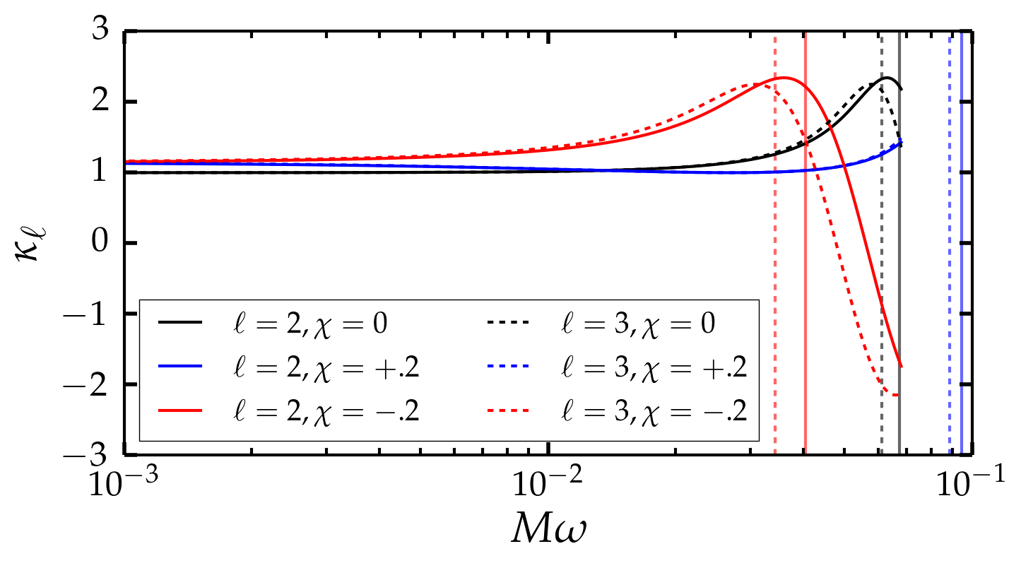
Figure 1: The dynamical tide amplification $\kappa_{\ell}$ from Eq. (26) modified by Eq. (43), as a function of orbital frequency, for the nonspinning case (black) and the spin aligned/antialigned (blue/red) cases for both $\ell=2$ (solid curves) and $\ell=3$ (dashed curves) tidal deformabilities. The vertical lines represent the resonance frequencies of both modes in every case. The parameters correspond to an NS with $\bar{\lambda}_{2}\approx 800$ in an equal mass system with total mass $2.8M_{\odot}$. For this NS, a spin magnitude of $|\chi_{\text{NS}}|=0.2$ corresponds to a rotational frequency of $f_{\text{NS}}\approx 312$Hz.

The dynamical tidal corrections discussed earlier in Sec. II.5 do not take into account the spin of the NS. The dynamical tides are caused by the changing tidal field due to the orbital motion interacting with the internal $f$-modes of the deformable object. So when the object is also spinning, its internal modes will effectively experience a driving frequency equal to the orbital frequency shifted by the object’s rotational frequency. We characterize this frequency shift by making a slight correction to the characteristic parameter $\gamma_{\ell A}$ in Eq. (25).

Given an aligned or antialigned spin of $\chi_{A}$ and a moment of inertia $I_{A}$, then we can compute the rotation frequency of the deformable object as

$$\bar{\omega}_{A}=M\omega_{A}=\frac{\chi_{A}}{X_{A}\bar{I}_{A}},$$ (41)

where the dimensionless moment of inertia is

$$\bar{I}_{A}= \frac{I_{A}}{m_{A}^{3}}.$$ (42)

Thus, the effective orbital frequency the resonant modes will experience is simply the difference between the orbital frequency and the rotational frequency of the object. With that in mind, we rewrite $\gamma_{\ell A}$ as

$$\gamma_{\ell A}=\left|\frac{\ell\left(v^{3}-\bar{\omega}_{A}\right)}{\bar{\omega}_{f\ell A}}\right|.$$ (43)

We take the absolute value because Eq. (25) is undefined for negative values of $\gamma_{\ell A}$, which can occur at low orbital frequencies with aligned spin objects. This corresponds to saying that the resonance modes of the object only care about the magnitude of the frequency of the changing tidal field. Within Eq. (28), we also need to make the change $\omega\rightarrow\left|v^{3}-\bar{\omega}_{A}\right|/M$.

To show how spin affects the profile of the dynamical tide correction, in Fig 1 we plot the profile of $\kappa_{\ell}$ from Eq. (26) as a function of orbital frequency. We assume an NS with $\bar{\lambda}_{2}\approx 800$ in an equal mass system and use the universal relations (see Table 2) to compute the other relevant tidal parameters. We compare the nonspinning NS against both aligned and antialigned spinning NS with magnitude $|\chi_{\text{NS}}|=0.2$, which corresponds to a rotational frequency of $f_{\text{NS}}\approx 312$Hz. The upper frequency termination point is at an orbital frequency of $M\omega_{\text{ISCO}}=6^{-3/2}$, which has been used as an approximate BNS inspiral termination criterion Bernuzzi et al. (2014).

From Fig 1 we can see that aligned spins push the resonance peak later in the inspiral while antialigned spins move the peak to smaller frequencies. In fact, with large enough aligned spins it is possible that the peak of the resonance is never reached before the system enters the merger/ringdown phase.

At low frequencies, the nonspinning system behaves the same as for static tides ($\kappa_{\ell}=1$). However, this is not true for the spinning systems, both of which asymptote to a slightly different value. Physically, these differences are due to the deformations of the object experiencing a driving frequency not from the orbital frequency (which is vanishingly small), but from its own rotation along its axis. We expect this difference to result in a negligible contribution to the waveform as the relative size of the tidal effects already vanishes [$\mathcal{O}(v^{10})$] at low frequencies. For the aligned spin object, note that there is a point in the evolution where the rotational and orbital frequencies match and the effective dynamical tidal field vanishes.

One concern is that for antialigned spins, $\kappa_{\ell}$ becomes negative before $M\omega_{\text{ISCO}}$. We recognize that Eq. (26) is derived assuming that the driving frequency is not much larger than the resonance peak Steinhoff et al. (2016). While for nonspinning systems and spin aligned systems the resonance peak occurs near the end of the inspiral or after merger/ringdown and is thus within the range of validity, that condition does not necessarily apply in the antialigned case. If the antialigned spin is large enough, as seems to be the case in Fig 1, the resonance frequency occurs early enough in the evolution that this approximate formalism potentially breaks down while still in the inspiral, necessitating a more delicate handling of the dynamical tides.

Until such a formalism is developed for antialigned NS spins, we instead assume for antialigned spin that the object is nonspinning (i.e., we set $\omega_{A}=0$) for the purposes of Eqs. (26) and (28); the aligned spin case will use Eq. (43) as expected.

IV Tidal Splicing

Putting together the results of the previous sections, we can write the PN equations of motion in the form

$$\frac{d\phi}{dt}= \frac{v^{3}}{M},$$ (44)

$$\frac{dv}{dt}= \mathcal{F}_{\text{BBH}}(v)+\mathcal{F}_{\text{Tid}}(v),$$ (45)

$$h^{\ell m}(t)= \left(A^{\ell m}_{\text{BBH}}(v)+A^{\ell m}_{\text{Tid}}(v)\right)e^{i(\psi^{\ell m}_{\text{BBH}}(v)-m\phi)},$$ (46)

where we have expressed the equations within the TaylorT4 framework. The expression for $\mathcal{F}_{\text{Tid}}(v)$ is given by Eq. (38), while $A^{\ell m}_{\text{BBH}}(v)$ and $\psi^{\ell m}_{\text{BBH}}(v)$ can be extracted from the expansions of Eq. (16) given in Blanchet et al. (2008) using the procedure we describe in Sec II.3. However, $\mathcal{F}_{\text{BBH}}(v)$, $A^{\ell m}_{\text{BBH}}(v)$ and $\psi^{\ell m}_{\text{BBH}}(v)$ are all unimportant for our purposes and so we do not present those formulas here.

Equivalently, the PN equations of motion can be written within the TaylorT2 framework as

$$t(v)= t_{0}+\mathcal{T}_{\text{BBH}}(v)+\mathcal{T}_{\text{Tid}}(v),$$ (47)

$$\phi(v)= \phi_{0}+\mathcal{P}_{\text{BBH}}(v)+\mathcal{P}_{\text{Tid}}(v),$$ (48)

$$h^{\ell m}(t)= \left(A^{\ell m}_{\text{BBH}}(v)+A^{\ell m}_{\text{Tid}}(v)\right)e^{i(\psi^{\ell m}_{\text{BBH}}(v)-m\phi)}.$$ (49)

The expression for $\mathcal{T}_{\text{Tid}}(v)$ and $\mathcal{P}_{\text{Tid}}(v)$ are given by Eqs. (39) and (40).

Consider the case of a BBH system. In principle, if we knew the PN expansions for the expressions of $\mathcal{F}_{\text{BBH}}$ (or $\mathcal{P}_{\text{BBH}}$ and $\mathcal{T}_{\text{BBH}}$), $A^{\ell m}_{\text{BBH}}$ and $\psi^{\ell m}_{\text{BBH}}$ up through arbitrarily large order, then we could perfectly reproduce the gravitational waveforms of those inspiraling systems. But unfortunately these terms are known only to a limited order.

However, numerical simulations of BBH systems are able to accurately solve the full Einstein equations. Thus, if we can represent these numerical waveforms in a form akin to the systems of equations in either Eqs. (44)-(46) or Eqs. (48) and (49) (with vanishing tidal terms), they would provide perfect representations of the PN expressions up to the numerical resolution error. This is the main idea of tidal splicing: We use numerical relativity BBH waveforms to effectively obtain the functions $\mathcal{F}_{\text{BBH}}(v)$,$\mathcal{P}_{\text{BBH}}(v)$, $\mathcal{T}_{\text{BBH}}(v)$, $A^{\ell m}_{\text{BBH}}(v)$, and $\psi^{\ell m}_{\text{BBH}}(v)$ to all orders in $v$. Then we add the analytic expressions for the tidal terms described above, and we integrate the PN equations of motion to generate waveforms corresponding to the inspirals of BHNS and BNS systems.

IV.1 Decomposition of NR waveforms

We start with a numerical BBH waveform corresponding to a system with a particular mass ratio $q$ and spins $\chi_{A}$ and $\chi_{B}$. The spins are assumed here to be aligned or antialigned with the orbital angular momentum. We decompose the $(2,2)$ mode of the BBH waveform in the form

$$h^{22}_{\text{NR}}(t)=A^{22}_{\text{NR}}(t)e^{-2i\phi_{\text{NR}}(t)},$$ (50)

where $A^{22}_{\text{NR}}(t)$ is real. This is the same decomposition as Eq. (20), so we interpret $\phi_{\text{NR}}(t)$ as the NR orbital phase. We then compute the effective PN expansion parameter $v_{\text{NR}}$ using Eq. (9):

$$v_{\text{NR}}(t)=\sqrt[3]{M\frac{d\phi_{\text{NR}}(t)}{dt}}.$$ (51)

Because the numerical waveform is known at a finite set of time samples, we use a sixth order finite difference scheme to compute the $d/dt$ derivatives numerically.

With the orbital phase and effective PN parameters in hand, we decompose each mode from the waveform into an amplitude and phase,

$$h^{\ell m}_{\text{NR}}(t)=A^{\ell m}_{\text{NR}}(t)e^{i\Phi^{\ell m}_{\text{NR}}(t)}.$$ (52)

Comparing with the expression for strain from Eq. (18), we break up the phase as

$$\Phi^{\ell m}_{\text{NR}}(t)=\psi^{\ell m}_{\text{NR}}(t)-m\phi_{\text{NR}}(t).$$ (53)

Since we know $\phi_{\text{NR}}$ we can compute $\psi^{\ell m}_{\text{NR}}$ from the total phase by rearranging Eq. (53),

$$\psi^{\ell m}_{\text{NR}}(t)=\Phi^{\ell m}_{\text{NR}}(t)+m\phi_{\text{NR}}(t).$$ (54)

Up to this point, we have been treating $t_{\text{NR}}$ as the independent variable for the purposes of decomposition. Since the PN formalism considers the frequency expansion parameter $v$ as the independent variable, we invert $v_{\text{NR}}(t)$ to get $t_{\text{NR}}(v)$ as a function of $v$. This inversion is straightforward numerically, since we have a finite number of time samples $t_{\text{NR}}$. Thus we can represent all of the individual parts of our waveform as functions of $v$, e.g., $\phi_{\text{NR}}(t_{\text{NR}}(v))=\phi_{\text{NR}}(v)$. Then we can write the strain for each mode in the form corresponding to Eq. (18):

$$h^{\ell m}_{\text{NR}}(v)= A^{\ell m}_{\text{NR}}(v)e^{i(\psi^{\ell m}_{\text{NR}}(v)-m\phi_{\text{NR}}(v))}.$$ (55)

We now have numerical equivalents for the various PN expansions for BBH systems; these are correct up to an arbitrary PN order and limited only by the errors from the simulations themselves.

IV.2 Tidal parameters

With the numerical decomposition in hand, we will need the tidal parameters for the particular BHNS or BNS system under consideration. A review of the different tidal effects explored in the previous section show there are six different parameters that characterize the tidal behavior of each object: the dimensionless quadrupolar and octopolar tidal deformabilities $\bar{\lambda}_{2}$ and $\bar{\lambda}_{3}$, their corresponding $f$-mode resonance frequencies $\omega_{f2}$ and $\omega_{f3}$, the dimensionless rotationally induced quadrupole moment $\bar{Q}$, and the dimensionless moment of inertia $\bar{I}$. For our model, we choose only $\bar{\lambda}_{2}$, and we compute the values of the other parameters from $\bar{\lambda}_{2}$ using the universal relations, which are approximate relations between $\bar{\lambda}_{2}$ and the other tidal parameters; the details are given in Appendix C. The choice of $\bar{\lambda}_{2}$ depends on the physical properties of the deformable object in consideration. Once we have chosen $\bar{\lambda}_{2}$ (and thus the other parameters via the universal relations), the next step in tidal splicing is the recomputation of the orbital evolution.

IV.3 Splicing of the orbital evolution equations

The details of how to specifically splice the PN tidal information into the orbital evolution depends on the specific Taylor expansion considered. We shall discuss the details of tidal splicing with TaylorT4 and TaylorT2. This method can also be performed for TaylorT3 Damour et al. (2001) which involves expanding about an intermediate dimensionless time variable. However, TaylorT3 is known to do a poor job in general of reproducing the results of BBH numerical simulations even in the equal mass, nonspinning case Boyle et al. (2007); Buonanno et al. (2009), so we ignore that method here. We also ignore TaylorT1 Damour et al. (2001) because we do not know how to compute the BBH contribution to the PN energy and flux separately using only the BBH waveform. While Ref. Barkett et al. (2016) discussed tidal splicing under a TaylorF2 Damour et al. (2000) framework, in this paper we only examine time domain approximants.

IV.3.1 TaylorT4 splicing

Splicing with TaylorT4, originally introduced within  Barkett et al. (2016), begins by examining how the tidal terms manifest in the TaylorT4 framework. The evolution of the PN parameter as seen in Eq. (45) for a BBH system is

$$\frac{dv}{dt}= \mathcal{F}_{\text{BBH}}(v).$$ (56)

With $t_{\text{NR}}(v)$ in hand from the simulation, we can compute a numerically accurate version of $\mathcal{F}_{\text{BBH}}(v)$ which we shall call $\mathcal{F}_{\text{NR}}(v)$,

$$\mathcal{F}_{\text{NR}}(v)=\left(\frac{dt_{\text{NR}}(v)}{dv}\right)^{-1}$$ (57)

The tidal terms, $\mathcal{F}_{\text{Tid}}(v_{\text{NR}})$, represent the sum of the additional tidal effects in the evolution and we compute them according to Eq. (70). We incorporate the dynamical tides by scaling the deformabilities according to Eq. (26), i.e., $\bar{\lambda}_{\ell}\rightarrow\bar{\lambda}_{\ell}\kappa_{\ell}(v)$.

We introduce a new spliced time coordinate, $t_{\text{Spl}}(v)$, which we compute by integrating the differential equation

$$\frac{dt_{\text{Spl}}}{dv}= \frac{1}{\mathcal{F}_{\text{NR}}(v)+\mathcal{F}_{\text{Tid}}(v)},$$ (58)

which is the inverse of Eq. (45). Once we have $t_{\text{Spl}}$, we find the orbital phase of this new waveform by integrating Eq. (44):

$$\phi_{\text{Spl}}(v)= \frac{1}{M}\int v(t_{\text{Spl}})^{3}dt_{\text{Spl}}.$$ (59)

We use Simpson’s method for integration. We choose the integration constants in Eqs. (58) and (59) to align the waveform to the numerical waveform at the initial time.

IV.3.2 TaylorT2 splicing

For BBH systems Eqs. (47) and (48) take the form

$$t(v)= t_{0}+\mathcal{T}_{\text{BBH}}(v),$$

$$\phi(v)= \phi_{0}+\mathcal{P}_{\text{BBH}}(v).$$ (60)

The constants $t_{0}$ and $\phi_{0}$ correspond simply to the starting time and phase of the waveform. Our numerically corrected versions of $\mathcal{T}_{\text{BBH}}$ and $\mathcal{P}_{\text{BBH}}$ are simply

$$\mathcal{T}_{\text{NR}}(v)= t_{\text{NR}}(v),$$

$$\mathcal{P}_{\text{NR}}(v)= \phi_{\text{NR}}(v).$$ (61)

We compute $\mathcal{T}_{\text{Tid}}(v)$ according to Eq. (71) and $\mathcal{P}_{\text{Tid}}(v)$ according to Eq. (72), incorporating the dynamical tides by making the frequency dependent adjustment to $\bar{\lambda}_{\ell}$ from Eq. (26).

The spliced waveform’s time $t_{\text{Spl}}$ and phase $\phi_{\text{Spl}}$ are then given by examining Eqs. (47) and (48) and making the appropriate substitutions,

$$t_{\text{Spl}}(v)= t_{0}+t_{\text{NR}}(v)+\mathcal{T}_{\text{Tid}}(v),$$

$$\phi_{\text{Spl}}(v)= \phi_{0}+\phi_{\text{NR}}(v)+\mathcal{P}_{\text{Tid}}(v).$$ (62)

We use the freedom inherent in choosing $t_{0}$ and $\phi_{0}$ to align the spliced waveform to the numerical waveform at the initial time

As the waveform nears the merger phase of the evolution, the effect from $\mathcal{T}_{\text{Tid}}(v)$ might grow larger than that of $t_{\text{NR}}(v)$. This may cause $t_{\text{Spl}}(v)$ to become nonmonotonic at some $v$; if this happens, we end the waveform at that value of $v$.

IV.4 Waveform reconstruction

Once $t_{\text{Spl}}(v)$ and $\phi_{\text{Spl}}(v)$ are computed, then the final step is reconstructing the spliced waveform from Eqs. (46) or (49) (which are the same equation). For $A^{\ell m}_{\text{BBH}}(v)$ and $\psi^{\ell m}_{\text{BBH}}(v)$ we use $A^{\ell m}_{\text{NR}}(v)$ and $\psi^{\ell m}_{\text{NR}}(v)$ computed from Eq. (55). For $A^{\ell m}_{\text{Tid}}(v)$ we use the expressions in Eq. (22), with the dynamical tides accounted for by the replacement rule $\bar{\lambda}_{2}\rightarrow\bar{\lambda}_{2A}\hat{\kappa}_{2A}(v)$ from Eq. (28). We thus arrive at the final formula for the spliced waveform modes:

$$h^{\ell m}_{\text{Spl}}\left(v\right)= \left(A^{\ell m}_{\text{NR}}(v)+A^{\ell m}_{\text{Tid}}(v)\right)e^{i(\psi^{\ell m}_{\text{NR}}(v)-m\phi_{\text{Spl}}(v))}.$$ (63)

To get a time-domain waveform, we invert the function $t_{\text{Spl}}(v)$. Because $v$ is known only at discrete values, we interpolate the amplitudes and phases of the waveforms onto a set of uniformly spaced values of $t_{\text{Spl}}$ using a cubic spline.

V Results

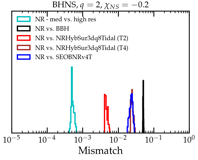
Figure 2: Distribution of mismatches across sky locations for the $q=2$, $\chi_{NS}=-0.2$ BHNS simulation. The cyan histogram show mismatches between waveforms from the highest two resolutions of the simulation, whereas all other histograms shows mismatches between the highest resolution waveform of the simulation versus the labeled waveform model. The BBH waveform model is the surrogate NRHybSur3dq8.

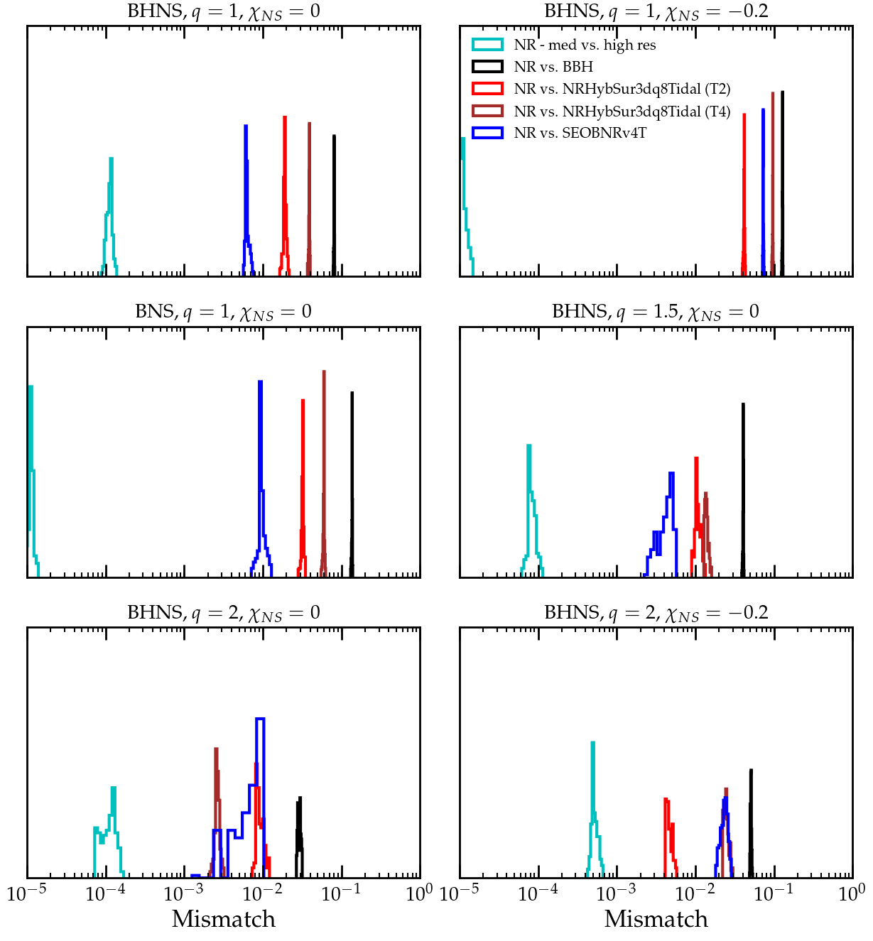
Figure 3: Distribution of mismatches across sky locations between the highest resolution waveform of the simulation versus the labeled waveform model for all six numerical simulations we consider.

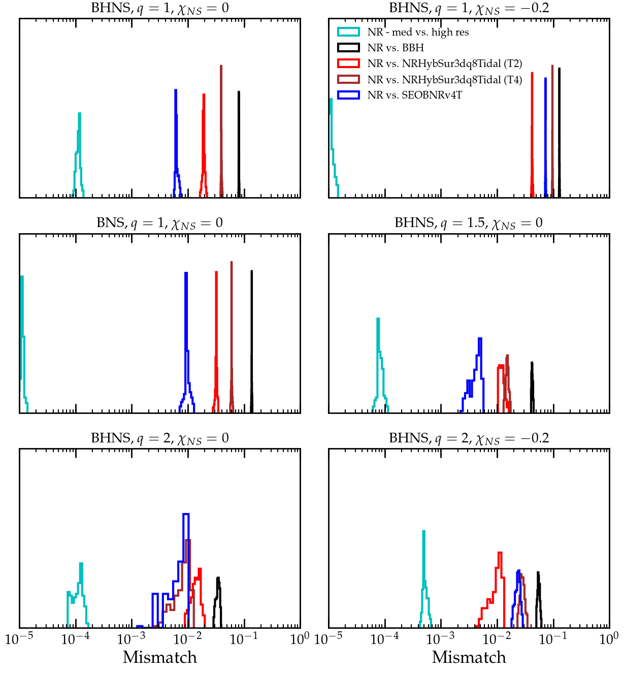
Figure 4: Distribution of mismatches across sky locations between the highest resolution waveform of the simulation versus the labeled waveform model for all six numerical simulations we consider, except that the BBH and tidally spliced waveforms are generated with only the (2,2) mode. See Sec. V.4 for discussion of higher-order modes.

V.1 Models for comparison

To measure the accuracy of the tidal splicing method, we compare our spliced waveforms against numerical simulations of BHNS/BNS inspirals. In particular, we use some of the recent numerical simulations from Foucart et al. (2019). In all simulations we compare against, the NSs were generated according to an EOS of $\Gamma=2$ polytrope with a mass $M_{\text{ADM}}=1.4M_{\odot}$ and compactness of $C_{\text{NS}}=0.1444$ so that the quadrupolar tidal deformability is $\bar{\lambda}_{2}\sim 800$. Comparing against one specific EOS at a single NS mass is a small slice of the full possible BHNS/BNS parameter space, but should give some idea for how well tidal splicing can perform. See Table 1 for the full list of the simulations we consider here. In particular, there are 1 BNS and 5 BHNS runs, and two of the BHNS runs have a small antialigned spin on the NS while the rest of the runs have zero spins.

We generated our tidally spliced waveforms for each of these cases using the hybridized surrogate model ‘NRHybSur3dq8’ Varma et al. (2019a) to compute the underlying BBH signal and making use of the universal relations to obtain the other tidal parameters from $\bar{\lambda}_{2}$; the details are given in Appendix C. The TaylorT2 splicing model has also been implemented as a tidal extension of “NRHybSur3dq8” under the name “NRHybSur3dq8Tidal”.

Type	$q$	$\chi_{\text{NS}}$	$f_{0}$ [Hz]	$f_{1}$ [Hz]	$N^{22}_{\text{cyc}}$
BHNS	1	0	218	578	19.9
BNS	1	0	211	629	20.8
BHNS	1	-0.2	217	505	17.0
BHNS	1.5	0	154	537	28.9
BHNS	2	0	156	505	21.0
BHNS	2	-0.2	156	485	19.8

Table 1: List of parameters for numerical simulations from Ref. Foucart et al. (2019) considered in this paper, namely the mass ratio $q$, the dimensionless spin of the neutron star $\chi_{\text{NS}}$, the lower and upper orbital frequency cutoffs of the waveforms $f_{0}$ and $f_{1}$, and the number of cycles in the (2,2) mode of the waveform between the cutoff frequencies.

To provide an additional point of comparison, we also test another waveform model, SEOBNRv4T, which is the time domain model SEOBNRv4 Bohé et al. (2017) augmented with most of the same effects we have used here, including higher-order corrections to the static tides in the EOB potential  Bini et al. (2012), strain corrections Baiotti et al. (2011), and dynamical tides (without the resonance frequency correction for spinning NSs) Hinderer et al. (2016). These effects correspond to our Eq. (66), Eq. (22), and Eqs. (26) and (28). This comparison is meant to serve as a proof of concept of tidal splicing against a similar model rather than a comprehensive survey of all models; we leave a more detailed comparison with other state-of-the-art models like TEOBResumS, LEA+, and the various extensions of the NRTidal model for future work.

V.2 Waveforms

The numerical waveforms we compare against include all modes through $\ell=5$, while the surrogate and spliced waveforms model only the modes [(2, 0), (2, 1), (2, 2), (3, 2), (3, 0), (3, 1), (3, 3), (4, 2), (4, 3), (4, 4), (5, 5)], and SEOBNRv4T models only the (2,2) mode. Since all systems we consider have spins parallel to the orbital angular momentum, we need only $m\geq 0$ modes; the $m<0$ modes are obtained from symmetry. The strain measured along a particular direction in the sky can then be written as

$$h_{+}(\iota,\varphi_{0})-ih_{\times}(\iota,\varphi_{0})=\sum_{\ell m}{h_{\ell m}}~{}_{-2}Y_{\ell m}(\iota,\varphi_{0})$$ (64)

Here ${}_{-2}Y_{\ell m}$ are spin-weighted spherical harmonics, and the angles $(\iota,\varphi_{0})$ are defined so that $\iota$ is the inclination angle between the binary angular momentum and the line of sight to the observer while $\varphi_{0}$ is the binary orbital phase when it enters the detector sensitivity band.

We choose the beginning of the waveform to be at a time after the initial burst of junk radiation, $t=200M$. That time also sets the starting orbital frequency of the waveform (chosen as half the time derivative of the phase of the (2,2) mode). To prevent the starting frequency $f_{\text{Initial}}$ from being contaminated by residual junk radiation in the imperfect BHNS/BNS initial data, we use a quadratic fit of the simulations’ frequency against time over the interval $t\in(200M,700M)$ to estimate the precise starting frequency. We window the waveform with a Planck-Taper window McKechan et al. (2010) over that early $500M$ region of the waveform. We label the orbital frequency at the end of this window as $f_{0}$; this frequency will serve as the initial frequency considered in our mismatches below.

At late times, we set the upper frequency cutoff $\omega_{\text{Cutoff}}$ by the frequency attained by the simulation at its peak power, and window the waveform (again with Planck-Taper) over the times from $f_{1}=0.85f_{\text{Cutoff}}$ to $f_{\text{Cutoff}}$. This gives us an inspiraling waveform from orbital frequency $f_{0}$ to $f_{1}$. The other waveforms we generated from $f_{\text{Initial}}$ to $f_{\text{Cutoff}}$ and windowed in a similar manner. In Table 1, we also list the number of cycles $N^{22}_{\text{cyc}}$ in the (2,2) mode of the numerical simulation within the listed orbital frequency bounds. While this is not necessarily a large frequency range to be making our comparisons, it is during the late inspiral where we expect the tidal effects to make the strongest contributions to the binary’s evolution.

After we transform all of the waveforms into the frequency domain, we calculate the mismatches with the numerical waveforms. To evaluate the mismatch, we optimize over time, orbital phase, and polarization angle shifts between the waveforms, following the procedure of Appendix D of Blackman et al. (2017a). We assume a flat noise spectrum. The starting and ending frequencies of the windowed waveforms, as given in Table 1, bound the frequency range for the mismatch computations. The mismatch between each of the models and the numerical simulation is then computed across 363 uniformly distributed sky locations.

We also attempted to evaluate a pair of frequency domain tidal waveform models, SEOBNRv4ROM_NRTidal and IMRPhenomD_NRTidal, but found mismatches between those models and the numerical simulations that we believed to be artificially large, near that of the BBH waveform. This is likely a consequence of having short numerical waveforms, which require windowing over a relatively short time interval, whereas the frequency-domain waveforms are not windowed. Note that all time-domain waveforms here are windowed in the same way, so systematic errors introduced by windowing should be the same for all of them. We have excluded the frequency domain waveforms from the results below.

V.3 Mismatch comparison: All modes

In Fig 2, we plot a histogram of mismatches against the numerical waveform across sky locations for a $q=2$, $\chi_{\text{NS}}=-0.2$ BHNS system. We do not normalize the vertical axis since the exact heights of the histograms are dependent on the binning choice; the locations of the histogram peaks correspond to how well the model does while the spread measures how dependent the model is on the sky location.

We estimate the numerical simulation error during the inspiral by the mismatch between simulations at the two highest numerical resolutions (cyan). Although this estimate is only a rough measure of the simulation error, and is possibly optimistic, the size of this mismatch suggests that the numerical error is smaller than the effects we are examining. Recall that we are not including merger and ringdown; the numerical error for the merger and postmerger evolution is expected to be much larger. The mismatch between the BHNS system and the surrogate BBH waveform (black) measures the strength of the tidal effects in the system, showing how poorly the waveforms will perform if tidal effects are neglected entirely.

As expected, both of the tidal splicing methods we try here, TaylorT4 (magenta) and TaylorT2 (red), improve upon the BBH waveform, as does the SEOBNRv4T model (blue). In this particular case, both the TaylorT4 and the SEOBNRv4T models show moderate improvements compared with the BBH waveform, accounting for some of the NSBH tidal effects, while the TaylorT2 model has mismatches about an order of magnitude smaller.

In Fig 3, we display the mismatch histograms across all simulations we consider. In all cases, the estimated numerical error of the inspiral is smaller than any of the mismatches from the waveforms considered here, and the size of the tidal effects behaves qualitatively as expected (i.e., more extreme mass ratios have smaller tidal effects, a spinning NS has larger tidal effects, …). The hierarchy between the TaylorT2 splicing, TaylorT4 splicing, and SEOBNRv4T changes across the parameter space, with each model performing the best in at least one of the cases.

In the case of low mass ratio ($q=1,1.5$), nonspinning BHNS and BNS (top left, middle left, and middle right), SEOBNRv4T has the lowest mismatches, followed by TaylorT2 splicing, and then TaylorT4 splicing. Across this region of the parameter space, there is very little change in behavior of the mismatches, with the BNS mismatches slightly larger, presumably because the tidal effects are at least twice as large (since both objects in the binary are being deformed rather than one). For nonspinning neutron stars, increasing the BHNS mass ratio from $q=1$ (top left) to $q=1.5$ (middle right) to $q=2$ (bottom left) shows relative improvement in the spliced waveforms, until in the $q=2$ case, the TaylorT4 splicing model has the smallest mismatches. The distribution of mismatches for SEOBNRv4T widens significantly with the increasing mass ratio, likely at least in part because of the growing significance of modes beyond (2,2), as we will discuss below.

The most significant change to the mismatches arises in the case of the spinning NS ($q=1$ top right; $q=2$ bottom right), where TaylorT2 splicing performs appreciably better than the other two models. In both cases, the mismatches of the waveforms worsen significantly compared to the corresponding nonspinning cases. At best, the effects included here only account for some of the changes the spinning NS has on the evolution of the system and on the gravitational radiation. Remaining errors in the tidal-splicing waveform models may be due to the missing spin-tidal terms (see Appendix D), the inaccurate handling of the dynamical tides in the case of antialigned NS, or some other unaccounted tidal effect. Further work will need to be done in order to properly capture the full behavior of systems with spinning NSs.

V.4 Mismatch comparison: (2,$\pm$2) Modes

The nonquadrupole modes are expected to become more important for systems with large mass ratios $q$ and/or large inclination angles $\iota$ Varma and Ajith (2017). In order to characterize how much of the disparity between the spliced and SEOBNRv4T waveforms is due to the inclusion of higher-order modes in the spliced models, we recompute the mismatches after restricting the BBH and spliced waveforms to only the $(2,\pm 2)$ modes (see Fig 4). The numerical simulations still utilize all the same modes as before.

For the nonspinning $q=1$ BHNS and BNS systems, there is very little change in the mismatches of the spliced waveforms when excluding the higher-order modes from the splicing model. This is expected, as a majority of the power in those waveforms is concentrated in the $(2,2)$ mode so leaving out the other modes produces a negligible effect. Thus the change in the histograms between Figs 3 and 4 for these systems is smaller than the width of the histograms. This also holds true for the equal mass spinning system and the $q=1.5$ system.

For the $q=2$ waveforms, restricting the splicing models to the $(2,\pm 2)$ modes leads to noticeably wider mismatch distributions. In the nonspinning case, the TaylorT4 splicing profile is similar to that of SEOBNRv4T, suggesting that much of the discrepancy between those two models in the bottom left panel of Fig.3 arises from the inclusion of higher-order modes. In the spinning case, while the TaylorT2 splicing waveform is wider than before, it still performs better than the other waveforms.

VI Conclusions

We have demonstrated how tidal splicing combines the accuracy of numerical BBH systems with the cheap computation of PN tidal formulas to generate waveforms corresponding to inspiraling BHNS and BNS systems. We expanded the tidal terms of the TaylorT2 and TaylorT4 PN approximants up to 2.5PN order and incorporated dynamical corrections to the approximants in order to improve our model. We also included a partial expansion of aligned spin-tidal corrections, though these additions are not complete to the same order as the nonspinning tidal effects. The tidal splicing method is now able to generate waveforms not only for the (2,2) mode, but for all modes supplied by the underlying BBH waveform. In particular, we applied tidal splicing to a surrogate model that spans the spin-aligned region of the BBH parameter space of interest to BNS and BHNS systems.

We measure the accuracy of tidal splicing against a series of inspiraling BNS and BHNS numerical simulations, and against the results of the SEOBNRv4T model. These simulations include systems with a mass ratio from $q=1$ to $q=2$ and both nonspinning and antialigned spin NSs. Across all cases, the tidally spliced waveforms capture an appreciable fraction of the tidal effects in the system. In different regions of the parameter space, different models perform best, with TaylorT4 splicing best in the $q=2$, nonspinning case, TaylorT2 splicing best in the spinning cases, and SEOBNRv4T best in the low mass ratio, nonspinning cases. We implement a model we call “NRHybSur3dq8Tidal”, which uses TaylorT2 splicing to extend the “NRHybSur3dq8” surrogate model for inspiraling tidal systems.

The accuracy of tidal splicing during the inspiral is limited in principle by the analytic tidal information fed into it, so the most natural extension of tidal splicing is through the inclusion of additional PN effects. As higher-order terms are computed, they can be appended to the TaylorT2 and TaylorT4 expressions. Adding more complete spin-tidal couplings and corrections to the dynamical tides would be particularly useful as the mismatches between the current spliced waveforms against the numerical simulations are worse for a spinning NS than for a nonspinning NS.

The current splicing method generates waveforms for only the inspiral portion of the signal, with no prescription for the merger and ringdown portions. Completing the full waveform will require developing a formalism for splicing BBH merger/ringdown signals, hybridizing the end portion with numerical results, or some other method. This is complicated by the fact that for BNS there are multiple possible final states (i.e., direct collapse to BH, long-lived hypermassive NS, …), each of which can imprint a unique signature on the merger/ringdown signal. We leave these possible improvements to future work.

Appendix A The 2.5PN Tidal Energy

Within the EOB framework, the energy terms associated with the quadrupolar and octopolar static deformations are known to 2PN Bini et al. (2012). We can convert these terms to an equivalent expression for the energy within the PN framework. For circular orbits, the full Hamiltonian is

$$H_{\text{EOB}}(u,J)= M\sqrt{1+2\nu\left(-1+\sqrt{\mathcal{A}(u)\left(1+\frac{J^{2}u^{2}}{m_{1}^{2}m_{2}^{2}}\right)}\right)},$$ (65)

where $u=M/r$ is the dimensionless inverse EOB radial coordinate, $J$ is the orbital angular momentum, and $\mathcal{A}(u)$ is the nonspinning radial PN potential, known through 2PN.

This $\mathcal{A}(u)$ is given in Bini et al. (2012), which we reproduce here for completeness,

$$\mathcal{A}(u)= \mathcal{A}_{\text{BBH}}(u)+\mathcal{A}_{\bar{\lambda}_{2}}(u)+\mathcal{A}_{\bar{\lambda}_{3}}(u),$$

$$\mathcal{A}_{\text{BBH}}(u)= 1-2u+2\nu u^{3}+\mathcal{O}(u^{4}),$$

$$\mathcal{A}_{\bar{\lambda}_{2}}(u)= 3\bar{\lambda}_{2A}X_{A}^{4}(1-X_{A})u^{5}\left(u+u^{2}\left(\frac{5}{2}X_{A}\right)+u^{3}\left(\frac{337}{28}X_{A}^{2}+\frac{1}{8}X_{A}+3\right)+\mathcal{O}(u^{4})\right)+(A\rightarrow B),$$

$$\mathcal{A}_{\bar{\lambda}_{3}}(u)= 3\bar{\lambda}_{3A}x_{A}^{6}(1-X_{A})u^{7}\left(u+u^{2}\left(\frac{15}{2}X_{A}-2\right)+u^{3}\left(\frac{110}{2}X_{A}^{2}-\frac{311}{24}X_{A}+\frac{8}{3}\right)+\mathcal{O}(u^{4})\right)+(A\rightarrow B).$$ (66)

The first unknown terms in $\mathcal{A}(u)$ are of order $\mathcal{O}(u^{3})$ beyond the leading order $1-2u$ Newtonian term, which corresponds to $\mathcal{O}(v^{6})$ beyond leading-order, or 3PN order. Since the tidal effects only enter at full PN orders, this potential is valid until to the first unknown terms at 3PN, i.e., up through 2.5PN.

To relate the EOB Hamiltonian to the PN energy expansions, we relate the EOB radial variable $u$ to the PN expansion variable $v$ via the orbital phase $\phi_{\text{orb}}$. Namely, $\phi_{\text{orb}}$ is both the conjugate variable of $p_{\phi}=J$, and one of the PN evolution equations as defined in Eq. (2). Therefore we establish the relationship between the EOB and PN energy equations with

$$\frac{\partial\phi_{\text{orb}}}{\partial t}= \frac{\partial H_{\text{EOB}}(u,J)}{\partial J}=\frac{v^{3}}{M}.$$ (67)

Because we are considering circular orbits, the radial conjugate variable $p_{u}$ is constant over the orbit, or $p_{u}=-\partial H_{\text{EOB}}(u,J)/\partial u=0$, which reduces to

$$0=\frac{\partial}{\partial u}\left(\mathcal{A}(u)\left(1+\frac{J^{2}u^{2}}{m_{1}^{2}m_{2}^{2}}\right)\right),$$ (68)

providing a relation between $J$ and $u$ Bini et al. (2012),

$$J^{2}=-\left(\frac{\partial\mathcal{A}(u)}{\partial u}\right)\bigg{/}\left(\frac{\partial\left(u^{2}\mathcal{A}(u)\right)}{\partial u}\right).$$ (69)

We can substitute this expression into Eq. (67), reducing the expression to a formula connecting $u$ and $v$, which we then expand to obtain $u$ as a power series of $v$. We then insert that expansion into the EOB Hamiltonian Eq, (65). By expressing the EOB Hamiltonian in powers of $v$, we obtain the PN energy formula given in Eq. (30), which is complete up through 2.5PN order.

Appendix B The 2.5PN Tidal Expressions

B.1 TaylorT4

Here we explicitly provide the full PN coefficients for the tidal terms in the TaylorT4 expansion in Eq. (38):

$$\mathcal{F}_{\text{Tid}}(v)= \frac{32\nu v^{9}}{5M}\left[\left(5(\bar{Q}_{A}-1)\chi_{A}^{2}X_{A}^{2}\right)v^{4}+\bar{\lambda}_{2A}X_{A}^{4}v^{10}\left(\sum^{5}_{i=0}\mathcal{F}_{2A,i}v^{i}\right)+\bar{\lambda}_{3A}X_{A}^{6}v^{14}\left(\sum^{5}_{i=0}\mathcal{F}_{3A,i}v^{i}\right)+\left(A\leftrightarrow B\right)\right],$$

$$\mathcal{F}_{2A,0}= 72-66X_{A},$$

$$\mathcal{F}_{2A,2}= \frac{4421}{56}-\frac{12263X_{A}}{56}+\frac{1893X_{A}^{2}}{4}-\frac{661X_{A}^{3}}{2},$$

$$\mathcal{F}_{2A,3}= 216\pi-216\pi X_{A}+\left(-\frac{1395X_{A}}{2}+\frac{753X_{A}^{2}}{2}+281X_{A}^{3}\right)\chi_{A}+\left(-\frac{1977}{2}+2228X_{A}-\frac{3041X_{A}^{2}}{2}+281X_{A}^{3}\right)\chi_{B},$$

$$\mathcal{F}_{2A,4}= \frac{130225}{96}+\alpha_{4}-\frac{853193X_{A}}{672}+\frac{664637X_{A}^{2}}{672}-\frac{249689X_{A}^{3}}{224}+\frac{5139X_{A}^{4}}{8}-\frac{12931X_{A}^{5}}{24}$$

$$+ \left(\frac{3915X_{A}^{2}}{8}-\frac{3771X_{A}^{3}}{8}+\bar{Q}_{A}\left(486X_{A}^{2}-468X_{A}^{3}\right)\right)\chi_{A}^{2}+\left(\frac{3861X_{A}}{4}-\frac{3789X_{A}^{2}}{2}+\frac{3717X_{A}^{3}}{4}\right)\chi_{A}\chi_{B}$$

$$+ \left(\frac{3915}{8}-\frac{11601X_{A}}{8}+\frac{11457X_{A}^{2}}{8}-\frac{3771X_{A}^{3}}{8}+\bar{Q}_{B}\left(486-1440X_{A}+1422X_{A}^{2}-468X_{A}^{3}\right)\right)\chi_{B}^{2},$$

$$\mathcal{F}_{2A,5}= \frac{50601\pi}{112}-\frac{154957\pi X_{A}}{112}+\frac{5267\pi X_{A}^{2}}{2}-\frac{6807\pi X_{A}^{3}}{4}$$

$$+ \left(-\frac{48145X_{A}}{14}+\frac{236779X_{A}^{2}}{84}-\frac{650371X_{A}^{3}}{168}+\frac{21111X_{A}^{4}}{8}+\frac{19277X_{A}^{5}}{12}\right)\chi_{A}$$

$$+ \left(-\frac{570401}{84}+\frac{849409X_{A}}{42}-\frac{4606397X_{A}^{2}}{168}+\frac{319379X_{A}^{3}}{14}-\frac{250409X_{A}^{4}}{24}+\frac{19277X_{A}^{5}}{12}\right)\chi_{B},$$

$$\mathcal{F}_{3A,0}= 520-520X_{A}+\beta_{0},$$

$$\mathcal{F}_{3A,2}= -\frac{14855}{21}+\frac{3\beta_{0}}{2}+\beta_{2}+X_{A}\left(\frac{62245}{21}+\frac{\beta_{0}}{6}\right)+\frac{X_{A}^{2}}{6}(3295-\beta_{0})-\frac{16835X_{A}^{3}}{6},$$

$$\mathcal{F}_{3A,3}= 2080\pi-2080\pi X_{A}+\left(-5X_{A}(1170+\beta_{0})-\frac{5}{3}X_{A}^{2}(-2002+\beta_{0})+\frac{7540X_{A}^{3}}{3}\right)\chi_{A}$$

$$+ \left(-\frac{10}{3}(2509+2\beta_{0})+X_{A}\left(19240+\frac{25\beta_{0}}{3}\right)-\frac{5}{3}X_{A}^{2}(8034+\beta_{0})+\frac{7540X_{A}^{3}}{3}\right)\chi_{B},$$

$$\mathcal{F}_{3A,4}= \frac{154460615}{18144}+\frac{99\beta_{0}}{8}+\frac{3\beta_{2}}{2}+\beta_{4}+X_{A}\left(-\frac{84699635}{18144}-\frac{53\beta_{0}}{8}+\frac{\beta_{2}}{6}\right)+X_{A}^{2}\left(-\frac{2405675}{672}+\frac{61\beta_{0}}{9}-\frac{\beta_{2}}{6}\right)$$

$$+ X_{A}^{3}\left(\frac{3298825}{224}-\frac{11\beta_{0}}{36}\right)+X_{A}^{4}\left(-7980+\frac{11\beta_{0}}{72}\right)-\frac{56095X_{A}^{5}}{8}$$

$$+ \left(X_{A}^{2}\left(\frac{8385}{2}+3\beta_{0}\right)-\frac{8385X_{A}^{3}}{2}+\bar{Q}_{A}\left(X_{A}^{2}(4160+3\beta_{0})-4160X_{A}^{3}\right)\right)\chi_{A}^{2}$$

$$+ \left(X_{A}(8255+6\beta_{0})-2X_{A}^{2}(8255+3\beta_{0})+8255X_{A}^{3}\right)\chi_{A}\chi_{B}$$

$$+ \bigg{[}\frac{8385}{2}+3\beta_{0}-\frac{3}{2}X_{A}(8385+4\beta_{0})+X_{A}^{2}\left(\frac{25155}{2}+3\beta_{0}\right)-\frac{8385X_{A}^{3}}{2}$$

$$+ \bar{Q}_{B}\left(4160+3\beta_{0}-6X_{A}(2080+\beta_{0})+3X_{A}^{2}(4160+\beta_{0})-4160X_{A}^{3}\right)\bigg{]}\chi_{B}^{2},$$

$$\mathcal{F}_{3A,5}= -\frac{121655\pi}{84}+\frac{328435\pi X_{A}}{84}+\frac{45980\pi X_{A}^{2}}{3}-\frac{53365\pi X_{A}^{3}}{3}$$

$$+ \bigg{[}X_{A}\left(-\frac{2284265}{168}-\frac{51\beta_{0}}{2}-5\beta_{2}\right)-\frac{5}{504}X_{A}^{2}(1874947+1260\beta_{0}+168\beta_{2})+X_{A}^{3}\left(-\frac{1280165}{56}-\frac{61\beta_{0}}{6}\right)$$

$$+ X_{A}^{4}\left(\frac{2816635}{72}+\frac{\beta_{0}}{6}\right)+\frac{573755X_{A}^{5}}{36}\bigg{]}\chi_{A}$$

$$+ \bigg{[}-\frac{5}{504}(3565057+672\beta_{2})-48\beta_{0}+X_{A}\left(\frac{9267085}{126}+\frac{241\beta_{0}}{3}+\frac{25\beta_{2}}{3}\right)$$

$$+ X_{A}^{2}\left(-42\beta_{0}-\frac{5}{252}(4784305+84\beta_{2})\right)+X_{A}^{3}\left(\frac{31907395}{252}+\frac{19\beta_{0}}{2}\right)+X_{A}^{4}\left(-\frac{6178195}{72}+\frac{\beta_{0}}{6}\right)+\frac{573755X_{A}^{5}}{36}\bigg{]}\chi_{B}.$$ (70)

Note that $\mathcal{F}_{2A,0}$ and $\mathcal{F}_{2A,2}$ reproduce the TaylorT4 coefficients from the quadrupolar deformability first computed in Ref Vines et al. (2011).

B.2 TaylorT2

Here we explicitly provide the full PN coefficients for the tidal terms in the TaylorT2 expansion in Eqs. (39) and (40). For the correction to the time, we find

$$\mathcal{T}_{\text{Tid}}(v)= -\frac{5M}{256\nu v^{8}}\left[-\left(10(\bar{Q}_{A}-1)\chi_{A}^{2}X_{A}^{2}\right)v^{4}+\bar{\lambda}_{2A}X_{A}^{4}v^{10}\left(\sum^{5}_{i=0}\mathcal{T}_{2A,i}v^{i}\right)+\bar{\lambda}_{3A}X_{A}^{6}v^{14}\left(\sum^{5}_{i=0}\mathcal{T}_{3A,i}v^{i}\right)+\left(A\leftrightarrow B\right)\right],$$

$$\mathcal{T}_{2A,0}= 288-264X_{A},$$

$$\mathcal{T}_{2A,2}= \frac{3179}{4}-\frac{919X_{A}}{4}-\frac{1143X_{A}^{2}}{2}+65X_{A}^{3},$$

$$\mathcal{T}_{2A,3}= -576\pi+\frac{2496\pi X_{A}}{5}+\left(324X_{A}+12X_{A}^{2}-\frac{1096X_{A}^{3}}{5}\right)\chi_{A}+\left(588-\frac{6616X_{A}}{5}+\frac{4772X_{A}^{2}}{5}-\frac{1096X_{A}^{3}}{5}\right)\chi_{B},$$

$$\mathcal{T}_{2A,4}= \frac{70312133}{21168}+\frac{4\alpha_{4}}{3}-\frac{147794303X_{A}}{127008}-\frac{20905X_{A}^{2}}{28}-\frac{432193X_{A}^{3}}{504}-\frac{5848X_{A}^{4}}{9}+\frac{857X_{A}^{5}}{3}$$

$$+ \left(-\frac{639X_{A}^{2}}{2}+\frac{525X_{A}^{3}}{2}+\bar{Q}_{A}\left(-312X_{A}^{2}+256X_{A}^{3}\right)\right)\chi_{A}^{2}+\left(-609X_{A}+1108X_{A}^{2}-499X_{A}^{3}\right)\chi_{A}\chi_{B}$$

$$+ \left(-\frac{639}{2}+\frac{1803X_{A}}{2}-\frac{1689X_{A}^{2}}{2}+\frac{525X_{A}^{3}}{2}+\bar{Q}_{B}\left(-312+880X_{A}-824X_{A}^{2}+256X_{A}^{3}\right)\right)\chi_{B}^{2},$$

$$\mathcal{T}_{2A,5}= -\frac{241295\pi}{98}+\frac{216921\pi X_{A}}{98}-\frac{7528\pi X_{A}^{2}}{7}+\frac{7142\pi X_{A}^{3}}{7}$$

$$+ \left(\frac{101949X_{A}}{49}+\frac{48875X_{A}^{2}}{294}-\frac{78373X_{A}^{3}}{147}-\frac{3417X_{A}^{4}}{7}-\frac{2574X_{A}^{5}}{7}\right)\chi_{A}$$

$$+ \left(\frac{637447}{147}-\frac{1026647X_{A}}{98}+\frac{931999X_{A}^{2}}{98}-\frac{713938X_{A}^{3}}{147}+\frac{12977X_{A}^{4}}{7}-\frac{2574X_{A}^{5}}{7}\right)\chi_{B},$$

$$\mathcal{T}_{3A,0}= \frac{4}{3}(520+\beta_{0})-\frac{2080X_{A}}{3},$$

$$\mathcal{T}_{3A,2}= \frac{33440}{21}+\frac{995\beta_{0}}{168}+\beta_{2}+\left(\frac{24670}{7}+\frac{17\beta_{0}}{3}\right)X_{A}-\frac{17}{6}(1825+2\beta_{0})X_{A}^{2}+\frac{325X_{A}^{3}}{6},$$

$$\mathcal{T}_{3A,3}= -\frac{64}{9}(260+\beta_{0})\pi+\frac{16640\pi X_{A}}{9}+\left(\frac{20}{9}(260+3\beta_{0})X_{A}+\frac{16}{27}(195+7\beta_{0})X_{A}^{2}-\frac{2080X_{A}^{3}}{3}\right)\chi_{A}$$

$$+ \left(\frac{4}{27}(8580+73\beta_{0})-\frac{4}{27}\left(21840+101\beta_{0}\right)X_{A}+\frac{16}{27}(4485+7\beta_{0})X_{A}^{2}-\frac{2080X_{A}^{3}}{3}\right)\chi_{B},$$

$$\mathcal{T}_{3A,4}= \frac{35111473}{3969}+\frac{6080015\beta_{0}}{254016}+\frac{199\beta_{2}}{42}+\frac{4\beta_{4}}{5}+\left(\frac{68598877}{7938}+\frac{16999\beta_{0}}{840}+\frac{68\beta_{2}}{15}\right)X_{A}$$

$$+ \frac{(7215185-16319\beta_{0}-11424\beta_{2})X_{A}^{2}}{2520}+\left(-\frac{154907}{8}-\frac{2477\beta_{0}}{90}\right)X_{A}^{3}+\left(-\frac{3040}{3}+\frac{2477\beta_{0}}{180}\right)X_{A}^{4}+\frac{455X_{A}^{5}}{18}$$

$$+ \left(\left(-858-\frac{57\beta_{0}}{10}\right)X_{A}^{2}+858X_{A}^{3}+\bar{Q}_{A}\left(\left(-832-\frac{28}{5}\beta_{0}\right)X_{A}^{2}+832X_{A}^{3}\right)\right)\chi_{A}^{2}$$

$$+ \left(\left(-1612-11\beta_{0}\right)X_{A}+\left(3224+11\beta_{0}\right)X_{A}^{2}-1612X_{A}^{3}\right)\chi_{A}\chi_{B}$$

$$+ \left[-858-\frac{57\beta_{0}}{10}+\left(2574+\frac{57}{5}\beta_{0}\right)X_{A}+\left(-2574-\frac{57\beta_{0}}{10}\right)X_{A}^{2}+858X_{A}^{3}\right.$$

$$~{}~{}~{}+\left.\bar{Q}_{B}\left(-832-\frac{28\beta_{0}}{5}+\left(2496+\frac{56\beta_{0}}{5}\right)X_{A}-\frac{4}{5}(3120+7\beta_{0})X_{A}^{2}+832X_{A}^{3}\right)\right]\chi_{B}^{2},$$

$$\mathcal{T}_{3A,5}= -\frac{1}{462}(2604260+17705\beta_{0}+2688\beta_{2})\pi+-\frac{2}{231}(516675+1687\beta_{0})\pi X_{A}+\frac{2}{33}(90640+241\beta_{0})\pi X_{A}^{2}+\frac{152360\pi X_{A}^{3}}{33}$$

$$+ \left[\frac{1}{924}(3242620+49273\beta_{0}+5040\beta_{2})X_{A}+\frac{(4691970+82637\beta_{0}+4704\beta_{2})X_{A}^{2}}{1386}+\frac{1}{693}(-221335+91\beta_{0})X_{A}^{3}\right.$$

$$~{}~{}~{}-\left.\frac{5}{99}(98807+254\beta_{0})X_{A}^{4}-\frac{156910X_{A}^{5}}{99}\right]\chi_{A}$$

$$+ \left[\frac{23393100+277897\beta_{0}+24528\beta_{2}}{2772}+\frac{(-44089360-337219\beta_{0}-33936\beta_{2})X_{A}}{2772}\right.$$

$$~{}~{}~{}\left.+\frac{(9394160-23497\beta_{0}+4704\beta_{2})X_{A}^{2}}{1386}+\left(-\frac{272870}{231}+\frac{563\beta_{0}}{11}\right)X_{A}^{3}-\frac{5}{99}(-68399+254\beta_{0})X_{A}^{4}-\frac{156910X_{A}^{5}}{99}\right]\chi_{B},$$ (71)

and for the correction to the phase we find

$$\mathcal{P}_{\text{Tid}}(v)= -\frac{1}{32\nu v^{5}}\left[-\left(25(\bar{Q}_{A}-1)\chi_{A}^{2}X_{A}^{2}\right)v^{4}+\bar{\lambda}_{2A}X_{A}^{4}v^{10}\left(\sum^{5}_{i=0}\mathcal{P}_{2A,i}v^{i}\right)+\bar{\lambda}_{3A}X_{A}^{6}v^{14}\left(\sum^{5}_{i=0}\mathcal{P}_{3A,i}v^{i}\right)+\left(A\leftrightarrow B\right)\right],$$

$$\mathcal{P}_{2A,0}= 72-66X_{A},$$

$$\mathcal{P}_{2A,2}= \frac{15895}{56}-\frac{4595X_{A}}{56}-\frac{5715X_{A}^{2}}{28}+\frac{325X_{A}^{3}}{14},$$

$$\mathcal{P}_{2A,3}= -225\pi+195\pi X_{A}+\left(\frac{2025X_{A}}{16}+\frac{75X_{A}^{2}}{16}-\frac{685X_{A}^{3}}{8}\right)\chi_{A}+\left(\frac{3675}{16}-\frac{4135X_{A}}{8}+\frac{5965X_{A}^{2}}{16}-\frac{685X_{A}^{3}}{8}\right)\chi_{B},$$

$$\mathcal{P}_{2A,4}= \frac{351560665}{254016}+\frac{5\alpha_{4}}{9}-\frac{738971515X_{A}}{1524096}-\frac{104525X_{A}^{2}}{336}-\frac{2160965X_{A}^{3}}{6048}-\frac{7310X_{A}^{4}}{27}+\frac{4285X_{A}^{5}}{36}$$

$$+ \left(-\frac{1065X_{A}^{2}}{8}+\frac{875X_{A}^{3}}{8}+\bar{Q}_{A}\left(-130X_{A}^{2}+\frac{320X_{A}^{3}}{3}\right)\right)\chi_{A}^{2}+\left(-\frac{1015X_{A}}{4}+\frac{1385X_{A}^{2}}{3}-\frac{2495X_{A}^{3}}{12}\right)\chi_{A}\chi_{B}$$

$$+ \left(-\frac{1065}{8}+\frac{3005X_{A}}{8}-\frac{2815X_{A}^{2}}{8}+\frac{875X_{A}^{3}}{8}+\bar{Q}_{B}\left(-130+\frac{1100X_{A}}{3}-\frac{1030X_{A}^{2}}{3}+\frac{320X_{A}^{3}}{3}\right)\right)\chi_{B}^{2},$$

$$\mathcal{P}_{2A,5}= -\frac{241295\pi}{224}+\frac{216921\pi X_{A}}{224}-\frac{941\pi X_{A}^{2}}{2}+\frac{3571\pi X_{A}^{3}}{8}$$

$$+ \left(\frac{101949X_{A}}{112}+\frac{48875X_{A}^{2}}{672}-\frac{78373X_{A}^{3}}{336}-\frac{3417X_{A}^{4}}{16}-\frac{1287X_{A}^{5}}{8}\right)\chi_{A}$$

$$+ \left(\frac{637447}{336}-\frac{1026647X_{A}}{224}+\frac{931999X_{A}^{2}}{224}-\frac{356969X_{A}^{3}}{168}+\frac{12977X_{A}^{4}}{16}-\frac{1287X_{A}^{5}}{8}\right)\chi_{B},$$

$$\mathcal{P}_{3A,0}= \frac{5}{9}(520+\beta_{0})-\frac{2600X_{A}}{9},$$

$$\mathcal{P}_{3A,2}= \frac{5(267520+995\beta_{0}+168\beta_{2})}{1848}+\left(\frac{123350}{77}+\frac{85\beta_{0}}{33}\right)X_{A}-\frac{85}{66}(1825+2\beta_{0})X_{A}^{2}+\frac{1625X_{A}^{3}}{66},$$

$$\mathcal{P}_{3A,3}= -\frac{10}{3}(260+\beta_{0})\pi+\frac{2600\pi X_{A}}{3}+\left(\frac{25}{24}(260+3\beta_{0})X_{A}+\frac{5}{18}(195+7\beta_{0})X_{A}^{2}-325X_{A}^{3}\right)\chi_{A}$$

$$+ \left(\frac{5}{72}(8580+73\beta_{0})-\frac{5}{72}\left(21840+101\beta_{0}\right)X_{A}+\frac{5}{18}(4485+7\beta_{0})X_{A}^{2}-325X_{A}^{3}\right)\chi_{B},$$

$$\mathcal{P}_{3A,4}= \frac{25(2247134272+6080015\beta_{0}+1203552\beta_{2})}{13208832}+\frac{5\beta_{4}}{13}+\left(\frac{1714971925}{412776}+\frac{84995\beta_{0}}{8736}+\frac{85\beta_{2}}{39}\right)X_{A}$$

$$- \frac{5(-7215185+16319\beta_{0}+11424\beta_{2})X_{A}^{2}}{26208}-\frac{5(6970815+9908\beta_{0})X_{A}^{3}}{3744}+\frac{5(-182400+2477\beta_{0})X_{A}^{4}}{1872}+\frac{875X_{A}^{5}}{72}$$

$$+ \left(\left(-\frac{825}{2}-\frac{285\beta_{0}}{104}\right)X_{A}^{2}+\frac{825X_{A}^{3}}{2}+\bar{Q}_{A}\left(\left(-400-\frac{35\beta_{0}}{13}\right)X_{A}^{2}+400X_{A}^{3}\right)\right)\chi_{A}^{2}$$

$$+ \left(\left(-775-\frac{275\beta_{0}}{52}\right)X_{A}+\left(1550+\frac{275\beta_{0}}{52}\right)X_{A}^{2}-775X_{A}^{3}\right)\chi_{A}\chi_{B}$$

$$+ \left[-\frac{825}{2}-\frac{285\beta_{0}}{104}+\frac{15}{52}(4290+19\beta_{0})X_{A}+\left(\frac{-2475}{2}-\frac{285\beta_{0}}{104}\right)X_{A}^{2}+\frac{825X_{A}^{3}}{2}\right.$$

$$~{}~{}~{}+\left.\bar{Q}_{B}\left(-400-\frac{35\beta_{0}}{13}+\left(1200+\frac{70\beta_{0}}{13}\right)X_{A}+\left(-1200-\frac{35\beta_{0}}{13}\right)X_{A}^{2}+400X_{A}^{3}\right)\right]\chi_{B}^{2},$$

$$\mathcal{P}_{3A,5}= -\frac{5(2604260+17705\beta_{0}+2688\beta_{2})\pi}{4704}-\frac{5(516675+1687\beta_{0})\pi X_{A}}{1176}+\frac{5}{168}(90640+241\beta_{0})\pi X_{A}^{2}+\frac{95225\pi X_{A}^{3}}{42}$$

$$+ \left[\frac{5(3242620+49273\beta_{0}+5040\beta_{2})X_{A}}{9408}+\frac{5(4691970+82637\beta_{0}+4704\beta_{2})X_{A}^{2}}{14112}+\frac{5(-221335+91\beta_{0})X_{A}^{3}}{7056}\right.$$

$$~{}~{}~{}-\left.\frac{25(98807+254\beta_{0})X_{A}^{4}}{1008}-\frac{392275X_{A}^{5}}{504}\right]\chi_{A}$$

$$+ \left[\frac{5(23393100+277897\beta_{0}+24528\beta_{2})}{28224}-\frac{5(44089360+337219\beta_{0}+33936\beta_{2})X_{A}}{28224}\right.$$

$$~{}~{}~{}+\left.\frac{5(9394160-23497\beta_{0}+4704\beta_{2})X_{A}^{2}}{14112}+\frac{5(-272870+11823\beta_{0})X_{A}^{3}}{2352}-\frac{25(-68399+254\beta_{0})X_{A}^{4}}{1008}-\frac{392275X_{A}^{5}}{504}\right]\chi_{B}.$$ (72)

Appendix C Model Parameters

$x$	$y$	$a_{0}$	$a_{1}$	$a_{2}$	$a_{3}$	$a_{4}$	Ref
$\bar{\lambda}_{2}$	$\ln\bar{Q}$	0.194	0.0936	0.0474	$-4.21\times 10^{-3}$	$1.23\times 10^{-4}$	Yagi and Yunes (2013a, b)
$\bar{\lambda}_{2}$	$\ln\bar{I}$	1.47	0.0817	0.0149	$2.87\times 10^{-4}$	$-3.64\times 10^{-5}$	Yagi and Yunes (2013a, b)
$\bar{\lambda}_{2}$	$\ln\bar{\lambda}_{3}$	$-1.15$	1.18	$-0.0251$	$-1.31\times 10^{-3}$	$2.52\times 10^{-5}$	Yagi (2014)
$\bar{\lambda}_{2}$	$X_{A}\bar{\omega}_{f2}$	0.1820	$-6.836\times 10^{-3}$	$-4.196\times 10^{-3}$	$5.215\times 10^{-4}$	$-1.857\times 10^{-5}$	Chan et al. (2014)
$\bar{\lambda}_{3}$	$X_{A}\bar{\omega}_{f3}$	0.2245	$-0.01500$	$-1.412\times 10^{-3}$	$1.832\times 10^{-4}$	$-5.561\times 10^{-6}$	Chan et al. (2014)

Table 2: Universal relations relating the static dimensionless deformability to various other dimensionless tidal parameters using Eq (73).

To serve as our underlying proxy for numerical BBH waveforms, we use the hybridized surrogate model “NRHybSur3dq8” Varma et al. (2019a). This model accurately captures the behavior of nonprecessing BBH systems for mass ratios up to $q=8$ with component spins $\chi\leq 0.8$ and including all of the following modes: [(2, 0), (2, 1), (2, 2), (3, 2), (3, 0), (3, 1), (3, 3), (4, 2), (4, 3), (4, 4), (5, 5)]. This region of parameter space spans the corresponding space of BNS and BHNS systems because the expected breakup spin for a neutron star is $\chi\sim 0.7$, and the tidal effects rapidly diminish for mass ratios significantly larger than unity (the leading-order tidal term in the Taylor expansions goes as $X_{A}^{4}$).

The tidal effects of each object are dependent on the object’s mass and the choice of EOS. There are currently six tidal parameters that enter into our model: the quadrupole and octopole static tidal deformabilities $\bar{\lambda}_{2}$ and $\bar{\lambda}_{3}$, their corresponding $f$-mode resonant frequencies $\bar{\omega}_{f2}$ and $\bar{\omega}_{f3}$, the dimensionless rotationally induced quadrupole moment $\bar{Q}$, and the dimensionless moment of inertia $\bar{I}$. (In Appendix D, we also briefly discuss how to include the four spin-tidal deformability parameters though they currently are not a part of our model.)

While in general, all of these parameters depend on the specific details of the object’s mass and EOS, recent analysis of these numbers show that the various parameters follow a series of universal relations that can accurately approximate their values given just $\bar{\lambda}_{2}$. The universal relations we use here all follow the same form Yagi and Yunes (2013a, b),

$$y= \sum_{i=0}^{4}a_{i}(\ln x)^{i},$$ (73)

where $x$ and $y$ are the two tidal parameters, and $a_{i}$ are the numerically fitted coefficients relating them (see Table 2). Thus, the properties of the NS of different theoretical EOS could be represented by how that EOS traces out the curve of allowable $\bar{\lambda}_{2}$ as a function of the mass of the NS. The extra factor of $X_{A}$ that appears as part of the dimensionless resonance frequencies $\bar{\omega}_{f\ell}$ in Table 2 arises because Ref. Chan et al. (2014) defines their dimensionless resonance frequency as $m_{A}\omega_{f\ell}$ whereas we use $\bar{\omega}_{f\ell}=M\omega_{f\ell}$.

Utilizing these universal relations reduces the effective parameter space of the tidal information from 12 (6 for each object) to just the static quadrupolar tidal deformability for each object, since all tidal parameters are derived simply from the choice of $\bar{\lambda}_{2}$. All together our spliced waveforms effectively fill a six-dimensional (6D) parameter space: $(q,M,\chi_{A},\chi_{B},\bar{\lambda}_{2A},\bar{\lambda}_{2B})$.

Equations (32) and (22) contain various currently unknown higher-order coefficients ($\alpha_{4}$ from the quadropolar tidal flux, $\beta_{0},\beta_{2},\beta_{4}$ from the octopolar tidal flux, and $\alpha^{22}_{4},\alpha^{21}_{2},\alpha^{33}_{2},\alpha^{31}_{2}$ from the tidal strain amplitude corrections) We set these coefficents to zero. Further study is needed in order to characterize the error associated with such a choice. In the case of the strain amplification corrections, we expect missing coefficients to be subdominant contributions to the signal according to Ref Damour et al. (2012).

Appendix D Spin-Tidal Connection Terms

In the expressions above, there are a number of terms that scale as $\bar{\lambda}_{2A}\chi_{A}$, so one might be tempted to view them as connections between the object’s tidal deformation and spin. Tracing back to the original energy and flux expressions, we know that instead these terms arise naturally as a consequence of power counting in the series expansion, and are merely cross terms between the tidal and spin-orbit or spin-spin effects.

Two different groups, Refs Abdelsalhin et al. (2018); Landry (2018), derived the first spin-tidal connection terms in the PN expansion. However, their two results are not consistent with each other, so we do not include either within our current splicing model. We do look at each paper and summarize how to implement either of these effects within our framework so that when this discrepancy is resolved, tidal splicing can be updated to include these terms.

The leading-order spin-tidal terms all enter at the $v^{13}$ order. There are four related effects that all enter at this order, each with its own dimensionless tidal deformability coefficient: $\bar{\lambda}_{23}$, the mass quadrupole tidal deformation arising due to the gravitomagnetic octopole tidal field; $\bar{\lambda}_{32}$, the mass octopole tidal deformation arising due to the gravitomagnetic quadrupole tidal field; $\bar{\sigma}_{23}$, the current quadrupole tidal deformation arising due to the gravitoelectric octopole tidal field; and $\bar{\sigma}_{32}$, the current octopole tidal deformation arising due to the gravitoelectric quadrupole tidal field.

To obtain the TaylorT terms, we examine leading-order terms in the PN energy and flux, and find

$$E_{\text{ST}}= -\frac{\nu v^{2}}{2}\left(1+v^{13}\chi_{A}X_{A}^{6}\sum_{i}\epsilon_{iA}\bar{\Lambda}_{iA}+(A\rightarrow B)\right),$$ (74)

$$F_{\text{ST}}= \frac{32\nu^{2}v^{10}}{5}\left(1+v^{13}\chi_{A}X_{A}^{6}\sum_{i}\rho_{iA}\bar{\Lambda}_{iA}+(A\rightarrow B)\right),$$ (75)

where the sums are over each of the ST parameters $\bar{\Lambda}_{iA}=(\bar{\lambda}_{23A},\bar{\lambda}_{32A},\bar{\sigma}_{23A},\bar{\sigma}_{32A})$, with energy coefficients $\epsilon_{iA}$ and flux coefficients $\rho_{iA}$ that are functions only of the mass fraction of the object $X_{A}$. In principle, we would need to include these energy and flux corrections into the full energy and flux equations, Eqs. (30) and (32).

We can expand Eqs. (74) and (75) in both the TaylorT4 and TaylorT2 manners yielding

$$\mathcal{F}_{\text{ST}}(v)= \frac{32\nu v^{9}}{5M}\left[v^{13}\chi_{A}X_{A}^{6}\sum_{i}\left(-\frac{15}{2}\epsilon_{iA}+\rho_{iA}\right)\bar{\Lambda}_{iA}\right],$$

$$\mathcal{T}_{\text{ST}}(v)= -\frac{5M}{256\nu v^{8}}\left[v^{13}\chi_{A}X_{A}^{6}\sum_{i}\left(-12\epsilon_{iA}+\frac{8}{5}\rho_{iA}\right)\bar{\Lambda}_{iA}\right],$$

$$\mathcal{P}_{\text{ST}}(v)= -\frac{1}{32\nu v^{5}}\left[v^{13}\chi_{A}X_{A}^{6}\sum_{i}\left(-\frac{75}{16}\epsilon_{iA}+\frac{5}{8}\rho_{iA}\right)\bar{\Lambda}_{iA}\right].$$ (76)

We can linearly add these expressions to the full tidal PN expressions $\mathcal{F}_{\text{Tid}}(v),\mathcal{T}_{\text{Tid}}(v)$, and $\mathcal{P}_{\text{Tid}}(v)$, respectively.

We now compare the energy and flux coefficients $\epsilon_{iA}$ and $\rho_{iA}$ as computed by Refs. Abdelsalhin et al. (2018); Landry (2018). In no particular order, we first examine Landry (2018), beginning with the correspondence between their (dimensionful) definitions of the deformability parameters,

$$\bar{\lambda}_{23}= m_{A}^{-6}\hat{\lambda}_{2},$$

$$\bar{\lambda}_{32}= m_{A}^{-6}\hat{\lambda}_{3},$$

$$\bar{\sigma}_{23}= -m_{A}^{-6}\hat{\sigma}_{2},$$

$$\bar{\sigma}_{32}= -m_{A}^{-6}\hat{\sigma}_{3},$$ (77)

where the parameters of Ref. Landry (2018) are hatted. From this we can write their energy and flux coefficients by reading off from Eqs. (28) and (30) of Landry (2018),

$$\epsilon_{iA}= \frac{44(1-X_{A})}{7X_{A}}\left(18,-2,-4,3\right),$$

$$\rho_{iA}= \left(144-\frac{204}{X_{A}},-16+\frac{16}{X_{A}},-38+\frac{113}{3X_{A}},24-\frac{24}{X_{A}}\right).$$ (78)

Repeating this same setup but with Abdelsalhin et al. (2018), we find the correspondence between their definitions and ours as

$$\bar{\lambda}_{23}= \frac{M^{2}}{m_{A}^{6}}\lambda_{23},$$

$$\bar{\lambda}_{32}= \frac{M^{2}}{m_{A}^{6}}\lambda_{32},$$

$$\bar{\sigma}_{23}= \frac{M^{2}}{m_{A}^{6}}\sigma_{23},$$

$$\bar{\sigma}_{32}= \frac{M^{2}}{m_{A}^{6}}\sigma_{32},$$ (79)

where the parameters of Ref. Abdelsalhin et al. (2018) are unbarred. Using their Eqs. (90) and (95),

$$\epsilon_{iA}= \frac{1-X_{A}}{X_{A}}\left(96,-32,-32,24\right),$$

$$\rho_{iA}= \left(96-\frac{136}{X_{A}},-32+\frac{32}{X_{A}},-38+\frac{113}{3X_{A}},24-\frac{24}{X_{A}}\right).$$ (80)

Appendix E $\bar{\lambda}_{2}\times\bar{\lambda}_{2}$ Self-Cross Terms

In the tidal PN formulations in this paper, the leading-order tidal terms are considered to be the same effective PN order as the Newtonian-order vacuum terms. Or in other words, we view $\mathcal{O}(\bar{\lambda}_{2}v^{10})\sim\mathcal{O}(1)$, so terms like $\bar{\lambda}_{2}v^{10}$ are treated as 0PN order, terms like $\bar{\lambda}_{2}v^{12}$ are treated as 1PN order, and so on, for the purposes of truncating the PN series. This means that terms like $\bar{\lambda}_{2}^{2}v^{20}$, $\bar{\lambda}_{2}^{3}v^{30}$, and so on can also in principle be considered 0PN order. So when multiplying or dividing PN series (for example, when dividing the two series on the right-hand side of Eq. (6)) and then truncating the series to a consistent PN order, the question arises as to whether one should eliminate terms of order $\mathcal{O}(\bar{\lambda}_{2}^{2}v^{20})$, $O(\bar{\lambda}_{2}^{3}v^{30})$, and so on. In this paper we do eliminate such terms, and we justify this choice in this appendix.

Note that the higher-order terms in question are not nonlinear static tidal terms (where the deformed tidal field of one object perturbs the tidal deformation of the other object) despite their appearance as such. These $\bar{\lambda}_{2}\times\bar{\lambda}_{2}$ terms are simply linear cross terms, such as the terms that go as $\bar{\lambda}_{2}\times\chi_{A,B}$ in Eqs. (70), (71), and (72), which are cross terms between spin-orbit and tidal contributions as opposed to spin-tidal effects.

Now while $v\rightarrow 0$, the assumption that $\mathcal{O}(\bar{\lambda}_{2}v^{10})\sim\mathcal{O}(1)$ is numerically not true, and instead we have $\mathcal{O}(\bar{\lambda}_{2}v^{10})\ll\mathcal{O}(1)$, so one could argue to neglect $\bar{\lambda}_{2}\times\bar{\lambda}_{2}$ terms. But as the binary approaches merger, and $v$ is no longer small, then we cannot assume $\mathcal{O}(\bar{\lambda}_{2}v^{10})\ll\mathcal{O}(1)$ holds true without further exploration.

To facilitate this discussion, we examine truncated versions of the PN energy and flux equations keeping just the leading-order BBH and tidal terms,

$$E(v)= -\frac{\nu v^{2}}{2}\left(1+9\bar{\lambda}_{2A}v^{10}X_{A}^{4}(-1+X_{A})\right.$$

$$+ \left.9\bar{\lambda}_{2B}v^{10}X_{B}^{4}(-1+X_{B})+\mathcal{O}(v)+\mathcal{O}(\bar{\lambda}_{2}v^{11})\right),$$

$$F(v)= \frac{32\nu^{2}v^{10}}{5}\left(1+6\bar{\lambda}_{2A}v^{10}X_{A}^{4}(3-2X_{A})\right.$$

$$+ \left.6\bar{\lambda}_{2B}v^{10}X_{B}^{4}(3-2X_{B})+\mathcal{O}(v)+\mathcal{O}(\bar{\lambda}_{2}v^{11})\right).$$

We now perform the PN series expansion in both the TaylorT4 and the TaylorT2 manners as in the rest of this paper, except we retain the next higher-order tidal cross terms,

$$\mathcal{F}_{\bar{\lambda}_{2}\times\bar{\lambda}_{2}}(v)= \frac{32\nu v^{9}}{5M}\left[1+v^{10}\left(\bar{\lambda}_{2A}X_{A}^{4}(72-66X_{A})+\bar{\lambda}_{2B}X_{B}^{4}(72-66X_{B})\right)+324v^{20}\left(\bar{\lambda}_{2A}^{2}X_{A}^{8}\left(12-23X_{A}+11X_{A}^{2}\right)\right.\right.$$

$$+ \left.\left.\bar{\lambda}_{2A}\bar{\lambda}_{2B}X_{A}^{4}X_{B}^{4}\left(24-23(X_{A}+X_{B})+22X_{A}X_{B}\right)+\bar{\lambda}_{2B}^{2}X_{B}^{8}\left(12-23X_{B}+11X_{B}^{2}\right)\right)\right.$$

$$+ \left.\mathcal{O}(v)+\mathcal{O}(\lambda_{2}v^{11})+\mathcal{O}(\lambda_{2}^{3}v^{30})\right],$$

$$\mathcal{T}_{\bar{\lambda}_{2}\times\bar{\lambda}_{2}}(v)= -\frac{5M}{256\nu v^{8}}\left[1+v^{10}\left(\bar{\lambda}_{2A}X_{A}^{4}(288-264X_{A})+\bar{\lambda}_{2B}X_{B}^{4}(288-264X_{B})\right)+24v^{20}\left(\bar{\lambda}_{2A}^{2}X_{A}^{8}\left(-36+57X_{A}-22X_{A}^{2}\right)\right.\right.$$

$$+ \left.\left.\bar{\lambda}_{2A}\bar{\lambda}_{2B}X_{A}^{4}X_{B}^{4}(-72+57(X_{A}+X_{B})-44X_{A}X_{B})+\bar{\lambda}_{2B}^{2}X_{B}^{8}(-36+57X_{B}-22X_{B}^{2})\right)\right.$$

$$+ \left.\mathcal{O}(v)+\mathcal{O}(\lambda_{2}v^{11})+\mathcal{O}(\lambda_{2}^{3}v^{30})\right],$$

$$\mathcal{P}_{\bar{\lambda}_{2}\times\bar{\lambda}_{2}}(v)= -\frac{1}{32\nu v^{5}}\left[1+v^{10}\left(\bar{\lambda}_{2A}X_{A}^{4}(72-66X_{A})+\bar{\lambda}_{2B}X_{B}^{4}(72-66X_{B})\right)+12v^{20}\left(\bar{\lambda}_{2A}^{2}X_{A}^{8}\left(-36+57X_{A}-22X_{A}^{2}\right)\right.\right.$$

$$+ \left.\left.\bar{\lambda}_{2A}\bar{\lambda}_{2B}X_{A}^{4}X_{B}^{4}(-72+57(X_{A}+X_{B})-44X_{A}X_{B})+\bar{\lambda}_{2B}^{2}X_{B}^{8}(-36+57X_{B}-22X_{B}^{2})\right)\right.$$

$$+ \left.\mathcal{O}(v)+\mathcal{O}(\lambda_{2}v^{11})+\mathcal{O}(\lambda_{2}^{3}v^{30})\right].$$ (82)

Compare with Eqs. (8),  (14), and (15), or with the equations in Appendix B.

	$\bar{\omega}_{\text{ISCO}}$	$\bar{\lambda}_{2}v_{\text{ISCO}}^{10}$	$\bar{\lambda}_{2}v_{\text{ISCO}}^{15}$	$\bar{\lambda}_{2}^{2}v_{\text{ISCO}}^{20}$	$\bar{\omega}_{\text{test}}$	$\bar{\lambda}_{2}v_{\text{test}}^{10}$	$\bar{\lambda}_{2}v_{\text{test}}^{15}$	$\bar{\lambda}_{2}^{2}v_{\text{test}}^{20}$
$\mathcal{F}_{\text{Tid}}(v)$	$6^{-3/2}$	0.313465	0.0588958	0.0680262	$6^{-3/2}/5$	$1.46652\times 10^{-3}$	$1.88467\times 10^{-5}$	$1.48894\times 10^{-6}$
$\mathcal{T}_{\text{Tid}}(v)$	$6^{-3/2}$	1.25386	$-0.4286$	$-0.0201559$	$6^{-3/2}/5$	$5.86608\times 10^{-3}$	$-1.37152\times 10^{-4}$	$-4.41166\times 10^{-7}$
$\mathcal{P}_{\text{Tid}}(v)$	$6^{-3/2}$	0.313465	$-0.187513$	$-0.0100779$	$6^{-3/2}/5$	$1.46652\times 10^{-3}$	$-6.0004\times 10^{-5}$	$-2.20583\times 10^{-7}$

Table 3: Magnitudes of the PN tidal self-cross terms from Eq. (82), assuming a fiducial system where $q=1,\chi_{A}=\chi_{B}=0,\bar{\lambda}_{2A}=1000,\bar{\lambda}_{2B}=0$, evaluated at two points in the inspiral, $\bar{\omega}_{\text{ISCO}}=6^{-3/2}$ and $\bar{\omega}_{\text{test}}=\bar{\omega}_{\text{ISCO}}/5$.

Because these cross terms will most strongly influence the waveform during the final stages of the inspirals, we estimate the size of the self-cross terms by comparing the magnitude of the various terms here at two different frequencies $\bar{\omega}_{\text{ISCO}}=6^{-3/2}$ and $\bar{\omega}_{\text{test}}=\bar{\omega}_{\text{ISCO}}/5$. We assume a fiducial binary system where $q=1,\chi_{A}=\chi_{B}=0,\bar{\lambda}_{2A}=1000,\bar{\lambda}_{2B}=0$. The results are displayed in Table 3. The columns labeled $\bar{\lambda}_{2}v^{10}$ and $\bar{\lambda}_{2}^{2}v^{20}$ in Table 3 correspond to the terms in Eqs (82). The columns labeled $\bar{\lambda}_{2}v^{15}$ correspond to the 2.5PN order $\bar{\lambda}_{2}$ terms [$\mathcal{F}_{2A,5}$ from Eq.(70), $\mathcal{T}_{2A,5}$ from Eq.(71), and $\mathcal{P}_{2A,5}$ from Eq.(72)], which serve as an error bound estimate arising from the unknown quadrupolar tidal terms. If the self-cross terms are larger than these, or near the size of the leading-order tidal terms, then we should not neglect the self-cross terms.

At the end of the waveform (i.e., at $\bar{\omega}_{\text{ISCO}}$), in the TaylorT4 case, the size of the self-cross terms is an appreciable fraction of the $\bar{\lambda}_{2}v^{10}$ term and the same size as the $\bar{\lambda}_{2}v^{15}$ term. This is also true in TaylorT2, but to a lesser extent, as the self-cross terms there are a factor of a few smaller. However, looking just a bit earlier in the inspiral we find that the self-cross terms drop off until they are distinctly smaller than even $\bar{\lambda}_{2}v^{15}$. Our general conclusion is that we are fine neglecting the self-cross terms for the time being, but as more tidal terms are introduced, we will eventually need to include these terms, especially to get the last orbits of the inspiral before the start of merger/ringdown.

This entire argument generalizes to the octopolar static tides, where the equivalent assumption is $\mathcal{O}(1)\sim\mathcal{O}(\bar{\lambda}_{3}v^{14})\sim\mathcal{O}(\bar{\lambda}_{3}^{2}v^{28})$, yet the octopolar effects are suppressed compared to the quadrupolar static tides. All of the arguments in favor of neglecting the $\mathcal{O}(\bar{\lambda}_{2}^{2}v^{20})$ terms should apply even more strongly to $\mathcal{O}(\bar{\lambda}_{3}^{2}v^{28})$, and so we ignore the $\mathcal{O}(\bar{\lambda}_{3}^{2}v^{28})$ terms as well.

References

- Aasi et al. (2015) J. Aasi et al. (LIGO Scientific Collaboration), Class. Quantum Grav. 32, 074001 (2015), arXiv:1411.4547 [gr-qc] .
- Acernese et al. (2015) F. Acernese et al. (Virgo Collaboration), Class. Quantum Grav. 32, 024001 (2015), arXiv:1408.3978 [gr-qc] .
- Abbott et al. (2017) B. P. Abbott et al. (Virgo, LIGO Scientific), Phys. Rev. Lett. 119, 161101 (2017), arXiv:1710.05832 [gr-qc] .
- Abbott et al. (2017) B. P. Abbott, R. Abbott, T. D. Abbott, F. Acernese, K. Ackley, C. Adams, T. Adams, P. Addesso, R. X. Adhikari, V. B. Adya, and et al., ”Astrophys. J. Lett.” 848, L13 (2017), arXiv:1710.05834 [astro-ph.HE] .
- Radice et al. (2018) D. Radice, A. Perego, F. Zappa, and S. Bernuzzi, The Astrophysical Journal Letters 852, L29 (2018), arXiv:1711.03647 [astro-ph.HE] .
- Del Pozzo et al. (2013) W. Del Pozzo, T. G. F. Li, M. Agathos, C. Van Den Broeck, and S. Vitale, Phys. Rev. Lett. 111, 071101 (2013), arXiv:1307.8338 [gr-qc] .
- Kumar et al. (2017) P. Kumar, M. Pürrer, and H. P. Pfeiffer, Phys. Rev. D95, 044039 (2017), arXiv:1610.06155 [gr-qc] .
- Vines et al. (2011) J. Vines, É. É. Flanagan, and T. Hinderer, Phys. Rev. D 83, 084051 (2011), arXiv:1101.1673 [gr-qc] .
- Chakravarti et al. (2019) K. Chakravarti et al., Phys. Rev. D99, 024049 (2019), arXiv:1809.04349 [gr-qc] .
- Samajdar and Dietrich (2018) A. Samajdar and T. Dietrich, Phys. Rev. D 98, 124030 (2018), arXiv:1810.03936 [gr-qc] .
- Messina et al. (2019) F. Messina, R. Dudi, A. Nagar, and S. Bernuzzi, Phys. Rev. D 99, 124051 (2019), arXiv:1904.09558 [gr-qc] .
- Damour and Nagar (2010) T. Damour and A. Nagar, Phys. Rev. D 81, 084016 (2010), arXiv:0911.5041 [gr-qc] .
- Hinderer et al. (2016) T. Hinderer et al., Phys. Rev. Lett. 116, 181101 (2016), arXiv:1602.00599 [gr-qc] .
- Steinhoff et al. (2016) J. Steinhoff, T. Hinderer, A. Buonanno, and A. Taracchini, Phys. Rev. D94, 104028 (2016), arXiv:1608.01907 [gr-qc] .
- Bohé et al. (2017) A. Bohé, L. Shao, A. Taracchini, A. Buonanno, S. Babak, I. W. Harry, I. Hinder, S. Ossokine, M. Pürrer, V. Raymond, T. Chu, H. Fong, P. Kumar, H. P. Pfeiffer, M. Boyle, D. A. Hemberger, L. E. Kidder, G. Lovelace, M. A. Scheel, and B. Szilágyi, Phys. Rev. D 95, 044028 (2017), arXiv:1611.03703 [gr-qc] .
- Bini et al. (2012) D. Bini, T. Damour, and G. Faye, Phys. Rev. D 85, 124034 (2012), arXiv:1202.3565 [gr-qc] .
- Baiotti et al. (2011) L. Baiotti, T. Damour, B. Giacomazzo, A. Nagar, and L. Rezzolla, Phys. Rev. D 84, 024017 (2011), arXiv:1103.3874 [gr-qc] .
- Dietrich and Hinderer (2017) T. Dietrich and T. Hinderer, Phys. Rev. D 95, 124006 (2017), arXiv:1702.02053 [gr-qc] .
- Nagar et al. (2018) A. Nagar et al., Phys. Rev. D 98, 104052 (2018), arXiv:1806.01772 [gr-qc] .
- Nagar et al. (2019) A. Nagar, F. Messina, P. Rettegno, D. Bini, T. Damour, A. Geralico, S. Akcay, and S. Bernuzzi, Phys. Rev. D 99, 044007 (2019), arXiv:1812.07923 [gr-qc] .
- Lackey et al. (2014) B. D. Lackey, K. Kyutoku, M. Shibata, P. R. Brady, and J. L. Friedman, Phys. Rev. D 89, 043009 (2014), arXiv:1303.6298 [gr-qc] .
- Taracchini et al. (2014) A. Taracchini et al., Phys. Rev. D89, 061502 (2014), arXiv:1311.2544 [gr-qc] .
- Dietrich et al. (2019a) T. Dietrich, S. Khan, R. Dudi, S. J. Kapadia, P. Kumar, A. Nagar, F. Ohme, F. Pannarale, A. Samajdar, S. Bernuzzi, G. Carullo, W. Del Pozzo, M. Haney, C. Markakis, M. Pürrer, G. Riemenschneider, Y. E. Setyawati, K. W. Tsang, and C. Van Den Broeck, Phys. Rev. D 99, 024029 (2019a), arXiv:1804.02235 [gr-qc] .
- Husa et al. (2016) S. Husa, S. Khan, M. Hannam, M. Pürrer, F. Ohme, X. Jiménez Forteza, and A. Bohé, Phys. Rev. D93, 044006 (2016), arXiv:1508.07250 [gr-qc] .
- Khan et al. (2016) S. Khan, S. Husa, M. Hannam, F. Ohme, M. Pürrer, X. Jiménez Forteza, and A. Bohé, Phys. Rev. D93, 044007 (2016), arXiv:1508.07253 [gr-qc] .
- Schmidt et al. (2012) P. Schmidt, M. Hannam, and S. Husa, Phys. Rev. D 86, 104063 (2012), arXiv:1207.3088 [gr-qc] .
- Schmidt et al. (2015) P. Schmidt, F. Ohme, and M. Hannam, Phys. Rev. D 91, 024043 (2015), arXiv:1408.1810 [gr-qc] .
- Dietrich et al. (2017) T. Dietrich, S. Bernuzzi, and W. Tichy, Phys. Rev. D96, 121501 (2017), arXiv:1706.02969 [gr-qc] .
- Dietrich et al. (2019b) T. Dietrich, A. Samajdar, S. Khan, N. K. Johnson-McDaniel, R. Dudi, and W. Tichy, Phys. Rev. D 100, 044003 (2019b), arXiv:1905.06011 [gr-qc] .
- Foucart et al. (2013) F. Foucart, L. Buchman, M. D. Duez, M. Grudich, L. E. Kidder, I. MacDonald, A. Mroue, H. P. Pfeiffer, M. A. Scheel, and B. Szilágyi, Phys. Rev. D 88, 064017 (2013), arXiv:1307.7685 [gr-qc] .
- Lovelace et al. (2013) G. Lovelace, M. D. Duez, F. Foucart, L. E. Kidder, H. P. Pfeiffer, M. A. Scheel, and B. Szilágyi, Class. Quantum Grav. 30, 135004 (2013), arXiv:1302.6297 [gr-qc] .
- Kawaguchi et al. (2015) K. Kawaguchi, K. Kyutoku, H. Nakano, H. Okawa, M. Shibata, and K. Taniguchi, Phys. Rev. D 92, 024014 (2015), arXiv:1506.05473 [astro-ph.HE] .
- Haas et al. (2016) R. Haas, C. D. Ott, B. Szilágyi, J. D. Kaplan, J. Lippuner, M. A. Scheel, K. Barkett, C. D. Muhlberger, T. Dietrich, M. D. Duez, F. Foucart, H. P. Pfeiffer, L. E. Kidder, and S. A. Teukolsky, Phys. Rev. D D93, 124062 (2016), arXiv:1604.00782 [gr-qc] .
- Hinderer et al. (2016) T. Hinderer, A. Taracchini, F. Foucart, A. Buonanno, J. Steinhoff, M. Duez, L. E. Kidder, H. P. Pfeiffer, M. A. Scheel, B. Szilágyi, K. Hotokezaka, K. Kyutoku, M. Shibata, and C. W. Carpenter, Phys. Rev. Lett. 116, 181101 (2016), arXiv:1602.00599 [gr-qc] .
- Dietrich et al. (2018) T. Dietrich, D. Radice, S. Bernuzzi, F. Zappa, A. Perego, B. Brügmann, S. V. Chaurasia, R. Dudi, W. Tichy, and M. Ujevic, Class. Quant. Grav. 35, 24LT01 (2018), arXiv:1806.01625 [gr-qc] .
- Foucart et al. (2019) F. Foucart et al., Phys. Rev. D99, 044008 (2019), arXiv:1812.06988 [gr-qc] .
- Kiuchi et al. (2020) K. Kiuchi, K. Kawaguchi, K. Kyutoku, Y. Sekiguchi, and M. Shibata, Phys. Rev. D 101, 084006 (2020), arXiv:1907.03790 [astro-ph.HE] .
- Aylott et al. (2009) B. Aylott et al., Class. Quantum Grav. 26, 114008 (2009), arXiv:0905.4227 [gr-qc] .
- Ajith et al. (2012) P. Ajith et al., Class. Quant. Grav. 29, 124001 (2012), [Erratum: Class. Quant. Grav.30,199401(2013)], arXiv:1201.5319 [gr-qc] .
- Hinder et al. (2014) I. Hinder et al. (The NRAR Collaboration), Class. Quantum Grav. 31, 025012 (2014), arXiv:1307.5307 [gr-qc] .
- Mroué et al. (2013) A. H. Mroué, M. A. Scheel, B. Szilágyi, H. P. Pfeiffer, M. Boyle, D. A. Hemberger, L. E. Kidder, G. Lovelace, S. Ossokine, N. W. Taylor, A. Zenginoğlu, L. T. Buchman, T. Chu, E. Foley, M. Giesler, R. Owen, and S. A. Teukolsky, Phys. Rev. Lett. 111, 241104 (2013), arXiv:1304.6077 [gr-qc] .
- Jani et al. (2016) K. Jani, J. Healy, J. A. Clark, L. London, P. Laguna, and D. Shoemaker, Class. Quant. Grav. 33, 204001 (2016), arXiv:1605.03204 [gr-qc] .
- Healy et al. (2017) J. Healy, C. O. Lousto, Y. Zlochower, and M. Campanelli, Classical and Quantum Gravity 34, 224001 (2017), arXiv:1703.03423 [gr-qc] .
- Healy et al. (2019) J. Healy, C. O. Lousto, J. Lange, R. O’Shaughnessy, Y. Zlochower, and M. Campanelli, Phys. Rev. D 100, 024021 (2019), arXiv:1901.02553 [gr-qc] .
- Huerta et al. (2019) E. A. Huerta, R. Haas, S. Habib, A. Gupta, A. Rebei, V. Chavva, D. Johnson, S. Rosofsky, E. Wessel, B. Agarwal, D. Luo, and W. Ren, Phys. Rev. D 100, 064003 (2019), arXiv:1901.07038 [gr-qc] .
- Boyle et al. (2019) M. Boyle et al., Class. Quantum Grav. 36, 195006 (2019), arXiv:1904.04831 [gr-qc] .
- Field et al. (2014) S. E. Field, C. R. Galley, J. S. Hesthaven, J. Kaye, and M. Tiglio, Phys. Rev. X 4, 031006 (2014), arXiv:1308.3565 [gr-qc] .
- Pürrer (2014) M. Pürrer, Class. Quantum Grav. 31, 195010 (2014), arXiv:1402.4146 [gr-qc] .
- Blackman et al. (2015) J. Blackman, S. E. Field, C. R. Galley, B. Szilágyi, M. A. Scheel, M. Tiglio, and D. A. Hemberger, Phys. Rev. Lett. 115, 121102 (2015), arXiv:1502.07758 [gr-qc] .
- Blackman et al. (2017a) J. Blackman, S. E. Field, M. A. Scheel, C. R. Galley, D. A. Hemberger, P. Schmidt, and R. Smith, Phys. Rev. D95, 104023 (2017a), arXiv:1701.00550 [gr-qc] .
- Blackman et al. (2017b) J. Blackman, S. E. Field, M. A. Scheel, C. R. Galley, C. D. Ott, M. Boyle, L. E. Kidder, H. P. Pfeiffer, and B. Szilágyi, Phys. Rev. D96, 024058 (2017b), arXiv:1705.07089 [gr-qc] .
- Varma et al. (2019a) V. Varma, S. E. Field, M. A. Scheel, J. Blackman, L. E. Kidder, and H. P. Pfeiffer, Phys. Rev. D99, 064045 (2019a), arXiv:1812.07865 [gr-qc] .
- Varma et al. (2019b) V. Varma, S. E. Field, M. A. Scheel, J. Blackman, D. Gerosa, L. C. Stein, L. E. Kidder, and H. P. Pfeiffer, Phys. Rev. Research 1, 033015 (2019b), arXiv:1905.09300 [gr-qc] .
- Barkett et al. (2016) K. Barkett, M. A. Scheel, R. Haas, C. D. Ott, S. Bernuzzi, D. A. Brown, B. Szilágyi, J. D. Kaplan, J. Lippuner, C. D. Muhlberger, F. Foucart, and M. D. Duez, Phys. Rev. D 93, 044064 (2016), arXiv:1509.05782 [gr-qc] .
- Blanchet (2014) L. Blanchet, Living Rev. Rel. 17, 2 (2014), arXiv:1310.1528 [gr-qc] .
- Fang and Lovelace (2005) H. Fang and G. Lovelace, Phys. Rev. D 72, 124016 (2005).
- Alvi (2001) K. Alvi, Phys. Rev. D 64, 104020 (2001).
- Flanagan and Hinderer (2008) É. É. Flanagan and T. Hinderer, Phys. Rev. D 77, 021502 (2008), arXiv:0709.1915 .
- Boyle et al. (2007) M. Boyle, D. A. Brown, L. E. Kidder, A. H. Mroue, H. P. Pfeiffer, M. A. Scheel, G. B. Cook, and S. A. Teukolsky, Phys. Rev. D76, 124038 (2007), arXiv:0710.0158 [gr-qc] .
- Damour et al. (2001) T. Damour, B. R. Iyer, and B. Sathyaprakash, Phys. Rev. D 63, 044023 (2001), arXiv:gr-qc/0010009 [gr-qc] .
- Blanchet et al. (2008) L. Blanchet, G. Faye, B. R. Iyer, and S. Sinha, Class. Quantum Grav. 25, 165003 (2008), arXiv:0802.1249 [gr-qc] .
- Blanchet and Schäfer (1993) L. Blanchet and G. Schäfer, Class. Quantum Grav. 10, 2699 (1993).
- Arun et al. (2004) K. G. Arun, L. Blanchet, B. R. Iyer, and M. S. S. Qusailah, Class. Quantum Grav. 21, 3771 (2004), arXiv:gr-qc/0404085 .
- Kidder (2008) L. E. Kidder, Phys. Rev. D 77, 044016 (2008), arXiv:0710.0614 [gr-qc] .
- Damour et al. (2012) T. Damour, A. Nagar, and L. Villain, Phys. Rev. D 85, 123007 (2012), arXiv:1203.4352 [gr-qc] .
- Jaranowski and Schäfer (1999) P. Jaranowski and G. Schäfer, Phys. Rev. D 60, 124003 (1999).
- de Andrade et al. (2001) V. C. de Andrade, L. Blanchet, and G. Faye, Class. Quantum Grav. 18, 753 (2001), arXiv:gr-qc/0011063 [gr-qc] .
- Blanchet and Faye (2001) L. Blanchet and G. Faye, Phys. Rev. D63, 062005 (2001), arXiv:gr-qc/0007051 [gr-qc] .
- Damour et al. (2001) T. Damour, P. Jaranowski, and G. Schäfer, Physics Letters B 513, 147 (2001), arXiv:gr-qc/0105038 .
- Blanchet et al. (2002) L. Blanchet, G. Faye, B. R. Iyer, and B. Joguet, Phys. Rev. D 65, 061501 (2002), erratum: Blanchet et al. (2005), arXiv:gr-qc/0105099 [gr-qc] .
- Blanchet et al. (2004) L. Blanchet, T. Damour, G. Esposito-Farese, and B. R. Iyer, Phys. Rev. Lett. 93, 091101 (2004), arXiv:gr-qc/0406012 [gr-qc] .
- Blanchet et al. (2006) L. Blanchet, A. Buonanno, and G. Faye, Phys. Rev. D 74, 104034 (2006).
- Kidder (1995) L. E. Kidder, Phys. Rev. D52, 821 (1995), arXiv:gr-qc/9506022 .
- Will and Wiseman (1996) C. M. Will and A. G. Wiseman, Phys. Rev. D54, 4813 (1996), arXiv:gr-qc/9608012 [gr-qc] .
- Poisson (1998) E. Poisson, Phys. Rev. D57, 5287 (1998), arXiv:gr-qc/9709032 .
- Bernuzzi et al. (2014) S. Bernuzzi, A. Nagar, S. Balmelli, T. Dietrich, and M. Ujevic, Phys. Rev. Lett. 112, 201101 (2014), arXiv:1402.6244 [gr-qc] .
- Buonanno et al. (2009) A. Buonanno, B. Iyer, E. Ochsner, Y. Pan, and B. S. Sathyaprakash, Phys. Rev. D80, 084043 (2009), arXiv:0907.0700 [gr-qc] .
- Damour et al. (2000) T. Damour, B. R. Iyer, and B. S. Sathyaprakash, Phys. Rev. D 62, 084036 (2000).
- McKechan et al. (2010) D. McKechan, C. Robinson, and B. Sathyaprakash, Class. Quantum Grav. 27, 084020 (2010), arXiv:1003.2939 [gr-qc] .
- Varma and Ajith (2017) V. Varma and P. Ajith, Phys. Rev. D96, 124024 (2017), arXiv:1612.05608 [gr-qc] .
- Yagi and Yunes (2013a) K. Yagi and N. Yunes, Phys. Rev. D 88, 023009 (2013a), arXiv:1303.1528 [gr-qc] .
- Yagi and Yunes (2013b) K. Yagi and N. Yunes, Science 341, 365 (2013b), arXiv:1302.4499 [gr-qc] .
- Yagi (2014) K. Yagi, Phys. Rev. D 89, 043011 (2014), errata: Yagi (2017),Yagi (2018), arXiv:1311.0872 [gr-qc] .
- Chan et al. (2014) T. K. Chan, Y.-H. Sham, P. T. Leung, and L.-M. Lin, Phys. Rev. D 90, 124023 (2014), arXiv:1408.3789 [gr-qc] .
- Abdelsalhin et al. (2018) T. Abdelsalhin, L. Gualtieri, and P. Pani, Phys. Rev. D 98, 104046 (2018), arXiv:1805.01487 [gr-qc] .
- Landry (2018) P. Landry, (2018), arXiv:1805.01882 [gr-qc] .
- Blanchet et al. (2005) L. Blanchet, G. Faye, B. R. Iyer, and B. Joguet, Phys. Rev. D 71, 129902 (2005).
- Yagi (2017) K. Yagi, Phys. Rev. D 96, 129904 (2017).
- Yagi (2018) K. Yagi, Phys. Rev. D 97, 129901 (2018).