Nonlinear force-free configurations in cylindrical geometry

Abstract

We find a new family of solutions for force-free magnetic structures in cylindrical geometry. These solutions have radial power-law dependance and are periodic but non-harmonic in azimuthal direction; they generalize the vacuum $z$-independent potential fields to current-carrying configurations.

1 Introduction

Force-free magnetic configurations, satisfying condition ${\bf B}=\kappa{\bf J}$, where ${\bf B}$ is magnetic field  and ${\bf J}$ is current density, are examples of magnetic structures that may represent the final stages of magnetic relaxation, or can be used as building block of plasma models (Lundquist, 1951; Woltier, 1958; Taylor, 1974; Priest & Forbes, 2000).

Particular linear examples of force-free equilibria, with spatially constant $\kappa$, were considered by Chandrasekhar & Kendall (1957). The most often-used configurations are Lundquist fields in cylindrical geometry (Lundquist, 1951) and spheromaks in spherical geometry (Bellan, 2000).

Using the self-similar assumption Lynden-Bell & Boily (1994) found non-linear self-similar solutions in spherical geometry. Their model of axially symmetric twisted configurations has been widely used in astrophysical and space applications ( Thompson et al., 2002; Shibata & Magara, 2011). In the spirit of Lynden-Bell & Boily (1994), in this paper we construct similar non-linear magnetic configurations in cylindrical geometry.

2 Self-similar configuration in cylindrical geometry

Shafranov (1966) and Grad (1967) formulated what is known as the Grad-Shafranov equation, separating complicated magnetic configuration in the set of nested/foliated flux surfaces, given by the condition that flux function $P$ is constant on the surface, and the encompassed current flow. Let us look for force-free equilibria that are independent of coordinate $z$. The two Euler potentials $\alpha$ and $\beta$ (or, equivalently, the related Clebsh variables) are

$$\alpha=z\mbox{}$$

$$\beta=P(r,\phi)$$ (1)

while the magnetic field can be written as

$${\bf B}=\nabla P\times\nabla z+g(P)\nabla z$$ (2)

where $g$ is some function.

Next we introduce a self-similar anzats

$$P(r,\phi)=r^{-l}f(\phi)\mbox{}$$

$$g(P)={\cal C}|P|^{p}\mbox{}$$

$${\bf B}=\nabla P\times\nabla z+{\cal C}|P|^{p}\nabla z=\{f^{\prime},lf,{\cal C}|f|^{p}\}r^{-(l+1)}$$ (3)

Absolute value of $|P|$ in the non-linear term ensures that magnetic field is real ($f(\phi)$ can become negative). Below any appearance of $f$ to non-integer power is to be understood to involve $\sqrt{f^{2}}=|f|$.

By dimensionality

$$p=1+1/l$$ (4)

Equation for $f$ becomes

$$lf^{\prime\prime}+l^{3}f+{\cal C}^{2}(1+l)f^{(2+l)/l}=0$$ (5)

(note that the component $B_{z}$ enters here as $B_{z}^{2}$. This justifies the use of $|P|$.)

For vacuum fields ${\cal C}=0$ the above relations reproduce

$$P\propto r^{-m}\sin(m\phi)\mbox{}$$

$$B_{r}\propto r^{-(1+m)}f^{\prime}\mbox{}$$

$$B_{\phi}\propto mr^{-(1+m)}f$$ (6)

with integer $m$.

The first integral is

$$f^{\prime,2}+l^{2}f^{2}+{\cal C}^{2}|f|^{2(1+l)/l}=H_{0},$$ (7)

By redefining $f\rightarrow\sqrt{H_{0}}f$ and ${\cal C}\rightarrow{\cal C}H_{0}^{-1/(2l)}$ the parameter $H_{0}$ can be set to unity,

$$f^{\prime,2}+l^{2}f^{2}+{\cal C}^{2}|f|^{2(1+l)/l}=1.$$ (8)

Equation (8) is the main equation describing non-linear force-free structures in cylindrical geometry. It depends on one parameter - the current strength ${\cal C}$. For a given ${\cal C}$ the value of $l$ is then determined as an eigenvalue problem by requiring periodicity in $\phi$, as we describe next.

We can solve for $f$ in quadratures:

$$\phi=\int\left(\sqrt{1-l^{2}f-{\cal C}^{2}|f|^{2(1+l)/l}}\right)^{-1}df$$ (9)

(so that the integration constant in Eq. (8) is just a phase $\phi$ where $f=0$).

Periodicity in $\phi$ requires

$$\int_{0}^{f_{max}}\left(\sqrt{1-l^{2}f-{\cal C}^{2}|f|^{2(1+l)/l}}\right)^{-1}df=\frac{\pi}{2m}$$ (10)

where $m=1,2..$ is an integer azimuthal number (see a comment after Eq. (16) why odd solutions, $\propto 2m+1$ in the denominator, are discarded), The value of $f_{max}$ satisfies

$$1-m^{2}f_{max}-{\cal C}^{2}f_{max}^{2(1+l)/l}=0$$ (11)

For given ${\cal C}$ the relations (10)- (11) constitute an eigenvalue problem on $l$. (For vacuum no current case ${\cal C}=0$ this reduces to $l=m$, an integer - checkmark.) In practice, we follow the following procedure: for each $m=1,2..$ we assume some $l$ and find ${\cal C}$ using relations (10)- (11). Thus, for each $m$ there is a continuous relation ${\cal C}(l)$. (Physically, of course, it is the current ${\cal C}$ the determines the radial index $l$.)

Results are plotted in Figs 2-3. In Fig. 2 we plot a particular solution for $l=1$ and $m=2$. The flux functions forms a ”petal” patter in azimuthal angle with number of ”petals” equal $2m$. There is a corresponding axial, unidirectional magnetic field $B_{z}$.

In Fig. 1 we plot the curves $l({\cal{C}})$ for various $m=2,4,6,8,10$. Each curve starts at a point $\{{\cal{C}}=0,l=2m\}$. For non-zero current ${\cal{C}}>0$ the radial dependence becomes more shallow, $l<2m$.

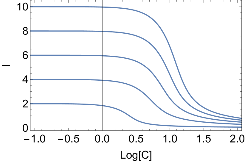
Figure 1: Dependence of the radial index $l$ on the current parameter ${\cal C}$ for various harmonics $m=2,4,6,8,10$.

In Fig. 3 we plot values of $\cal{C}$ as a function of azimuthal number $m$ for different values of $l=0.25...2$. Dashed lines are for convenience only, they connect points corresponding to the same radial parameter $l$.

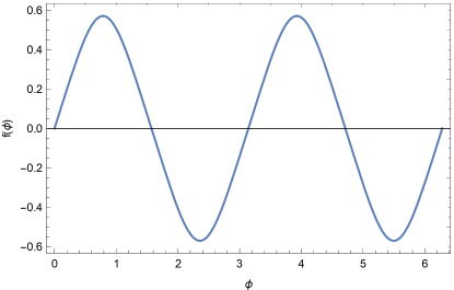
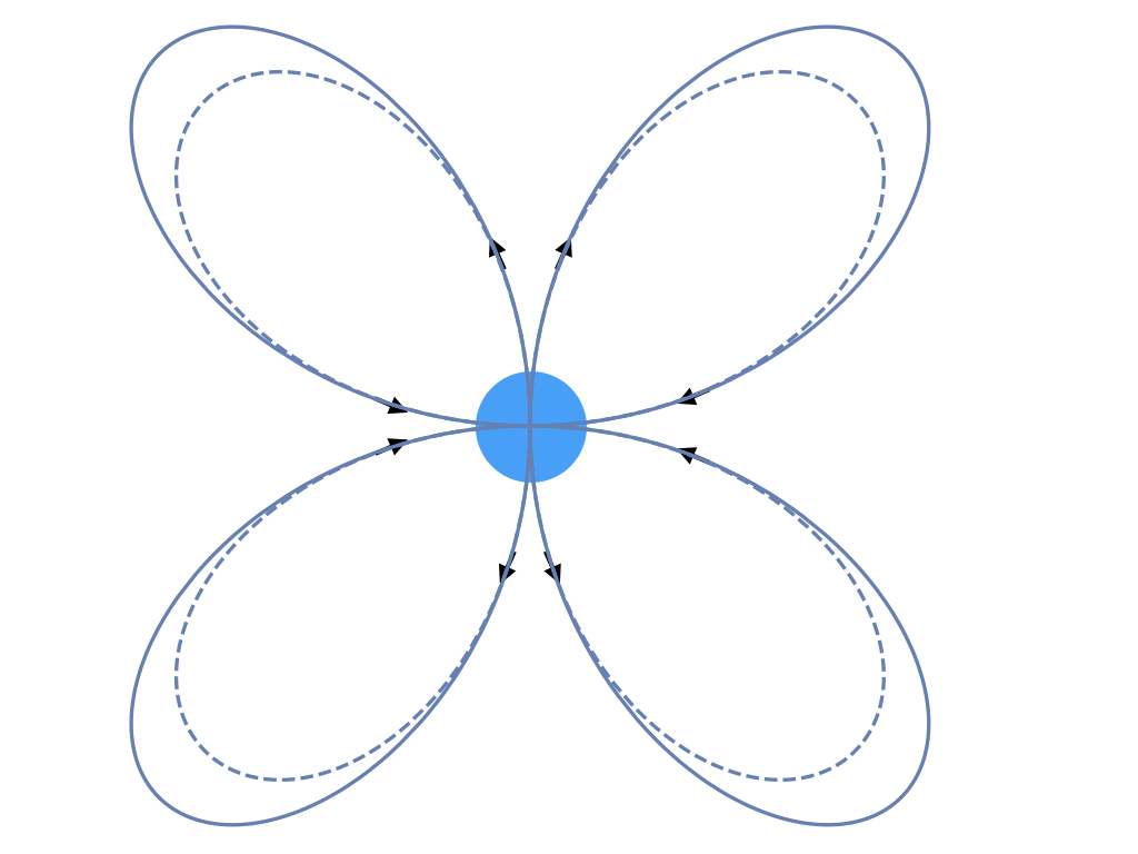
Figure 2: Left panel: example of solution $f(\phi)$ for $l=1$, $m=2$. In this case ${\cal C}=2.517$. Right panel: structure of poloidal field. (Due to the assumed self-similar radial structure the solutions do not extend to $r=0$). Dashed line is the corresponding vacuum case, Eq. 6.

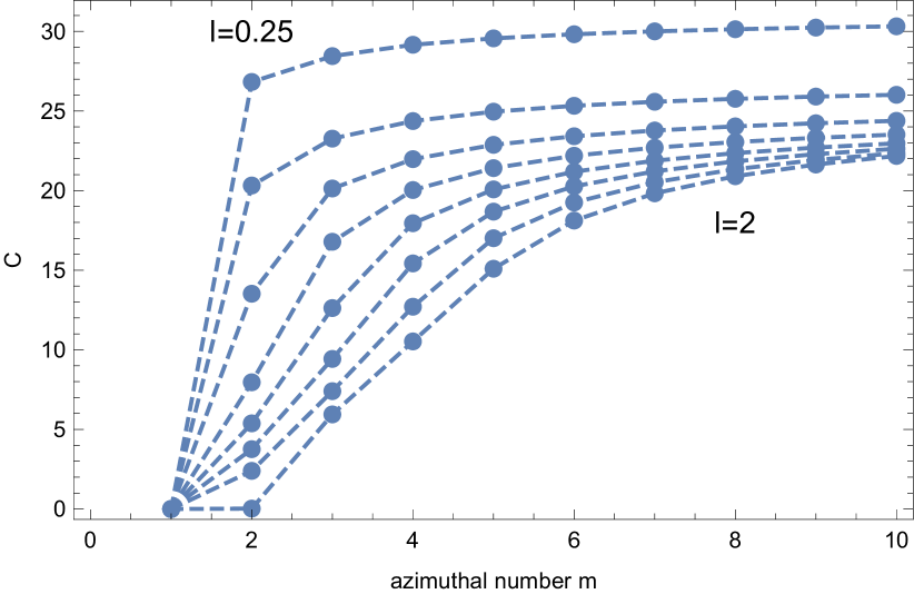
Figure 3: Values of $\cal{C}$ as a function of azimuthal number $m$ for different values of $l=0.25...2$ (in steps of $0.25$). Top curves correspond to smaller $l$.

3 Analysis of the solutions

In a formulation of force-free fields in the form

$${\rm curl\,}{\bf B}=\kappa{\bf B}$$ (12)

the value of $\kappa$ is

$$\kappa={\cal C}\frac{1+l}{lr}f^{1/l}$$ (13)

It is constant on flux surfaces $P$, Eq. 3.

The current density (we incorporate factors of $4\pi/c$ into definition of magnetic field)

$$j_{r}={\cal C}\frac{1+ll}{l}r^{-(l+2)}\partial_{\phi}\left(|f|\right)^{(1+l)/l}\mbox{}$$

$$j_{\phi}={\cal C}(l+1)r^{-(l+2)}\left(|f|\right)^{(1+l)/l}\mbox{}$$

$$j_{\phi}=r^{-(l+2)}\left(f^{\prime\prime}+l^{2}\right)=-{\cal C}^{2}\frac{1+ll}{l}r^{-(l+2)}\left(|f|\right)^{(2+l)/l}$$ (14)

The total axial current is

$$I_{z}=\int_{r_{0}}^{\infty}rdr\int_{0}^{2\pi}d\phi j_{z}=-\frac{r_{0}^{-l}}{l}\int_{0}^{2\pi}d\phi\left(f^{\prime\prime}+l^{2}f\right).$$ (15)

where $r_{0}$ is the inner boundary. The total axial current vanishes if two conditions are satisfied

$$\int_{0}^{2\pi}fd\phi=0\mbox{}$$

$$f^{\prime}(2\pi)=f^{\prime}(0)$$ (16)

All the solutions considered here satisfy these conditions: the second one requires even azimuthal numbers, $2m$. Generally, there is a larger family of self-similar force-free equilibria with non-zero total axial current.

There is non-zero toroidal current

$$j_{\phi}={\cal C}(l+1)r^{-2-l}|f|^{(1+l)/l}\mbox{}$$

$$\int_{0}^{2\pi}d\phi j_{\phi}\neq 0$$ (17)

The radial current density integrated over $\phi$ satisfies

$$j_{r}\propto\int_{0}^{2\pi}d\phi\partial_{\phi}\left(|f|\right)^{(1+l)/l}=\left.\left(|f|\right)^{(1+l)/l}\right|_{0}^{2\pi}=0$$ (18)

4 Discussion

In this paper we make analytical progress with the highly nonlinear problem[s] of magnetohydrodynamics (Lynden-Bell & Boily, 1994). We find a class of non-linear self-similar force-free equilibria in cylindrical geometry. The solutions we find all connect to the vacuum case, in which case the flux function is $P_{vac}\propto r^{-m}\sin(m\phi)$. Structures with vanishing total axial current require even values of $m$ (hence $m\rightarrow 2m$). For non-zero distributed current with the current parameter ${\cal C}$ the radial dependence changes to $r^{-l}$, with $l<2m$, while remaining periodic in $\phi$ at $2m$. Solutions for a given $m$ resemble vacuum solutions $\propto\sin(2m\phi)$, but they are not exactly harmonic in the nonlinear case.

For very large currents the solutions asymptote to $l\approx 0$, but never reach this limit. The case $l=0$ corresponds to $B_{r}\propto 1/r$. Mathematically, this is the analogue of split monopole case in the spherical geometry - split monopole case can be achieved in spherical geometry (with corresponding anti-monopole in the opposite hemisphere), but is not possible in the cylindrical geometry.

References

- Bellan (2000) Bellan, P. M. 2000 Spheromaks: a practical application of magnetohydrodynamic dynamos and plasma self-organization. Spheromaks: a practical application of magnetohydrodynamic dynamos and plasma self-organization/ Paul M. Bellan. London: Imperial College Press; River Edge, NJ: Distributed by World Scientific Pub. Co., c2000.
- Chandrasekhar & Kendall (1957) Chandrasekhar, S. & Kendall, P. C. 1957 On Force-Free Magnetic Fields. ApJ 126, 457–+.
- Grad (1967) Grad, H. 1967 Toroidal Containment of a Plasma. Physics of Fluids 10 (1), 137–154.
- Lundquist (1951) Lundquist, S. 1951 On the Stability of Magneto-Hydrostatic Fields. Phys. Rev. 83, 307–311.
- Lynden-Bell & Boily (1994) Lynden-Bell, D. & Boily, C. 1994 Self-Similar Solutions up to Flashpoint in Highly Wound Magnetostatics. MNRAS 267, 146.
- Priest & Forbes (2000) Priest, E. & Forbes, T. 2000 Magnetic Reconnection.
- Shafranov (1966) Shafranov, V. D. 1966 Plasma Equilibrium in a Magnetic Field. Reviews of Plasma Physics 2, 103–+.
- Shibata & Magara (2011) Shibata, K. & Magara, T. 2011 Solar Flares: Magnetohydrodynamic Processes. Living Reviews in Solar Physics 8 (1), 6.
- Taylor (1974) Taylor, J. B. 1974 Relaxation of Toroidal Plasma and Generation of Reverse Magnetic Fields. Phys. Rev. Lett. 33, 1139–1141.
- Thompson et al. (2002) Thompson, C., Lyutikov, M. & Kulkarni, S. R. 2002 Electrodynamics of Magnetars: Implications for the Persistent X-Ray Emission and Spin-down of the Soft Gamma Repeaters and Anomalous X-Ray Pulsars. ApJ 574 (1), 332–355, arXiv: astro-ph/0110677.
- Woltier (1958) Woltier, L. 1958 Proc. Nat. Acad. Sci. 44, 489.