Constrained Linear Data-feature Mapping
for Image Classification

Abstract

In this paper, we propose a constrained linear data-feature mapping model as an interpretable mathematical model for image classification using convolutional neural network (CNN) such as the ResNet. From this viewpoint, we establish the detailed connections in a technical level between the traditional iterative schemes for constrained linear system and the architecture for the basic blocks of ResNet. Under these connections, we propose some natural modifications of ResNet type models which will have less parameters but still maintain almost the same accuracy as these corresponding original models. Some numerical experiments are shown to demonstrate the validity of this constrained learning data-feature mapping assumption.

1 Introduction

This paper is devoted to providing some mathematical insight of deep convolutional neural network models that have been successfully applied in many machine learning and artificial intelligence areas such as computer vision, natural language precessing and reinforcement learning [24]. Important examples of CNN include the LeNet-5 model of LeCun et al. in 1998 [25], the AlexNet of Hinton et el in 2012 [22], Residual Network (ResNet) of K. He et al in 2015 [13] and Pre-act ResNet in 2016 [14], and other variants of CNN in [32, 37, 17]. Among these different CNNs, ResNet and pre-act ResNet models are of special theoretical and practical interests. It has been an active research topic on theoretical understanding or explanation of why and how ResNet work well, and how to design better residual type architectures based on certain empirical observations and formal interpretation, see [41, 23, 6, 38, 43, 36, 17]. For example, a dynamical system viewpoint was discussed in [28, 2] to explain the rational for skip connections in ResNets.

In this paper, we propose a generic mathematical model behind the residual blocks in ResNet to understand how ResNet model works. The core of our model is the following assumption: there is a data-feature mapping

$$A\ast u=f,$$ (1.1)

where $f$ is the data such as images we see and $u$ represents a feature tensor such that

$$u\geq 0.$$ (1.2)

Feature extraction is then viewed as an iterative procedure (c.f. [39]) to solve (1.1):

$$u^{i}=u^{i-1}+B^{i}\ast(f-A\ast u^{i-1}),\quad i=1:\nu.$$ (1.3)

Using, for example, the special activation function $\sigma(x)={\rm ReLU}(x):=\max\{0,x\}$, the above iterative process can be naturally modified to preserve the constraint (1.2):

$$u^{i}=u^{i-1}+\sigma\circ B^{i}\ast\sigma(f-A\ast u^{i-1}),\quad i=1:\nu.$$ (1.4)

Introducing the residual

$$r^{i}=f-A\ast u^{i},$$ (1.5)

the iterative process (1.4) can be written as

$$r^{i}=r^{i-1}-A\ast\sigma\circ B^{i}\ast\sigma(r^{i-1}),\quad i=1:\nu.$$ (1.6)

This above process represent one major modified pre-act ResNet to be studied in this paper and it can be directly compared with the following process representing a core component of pre-act ResNet [14]:

$$r^{i}=r^{i-1}-A^{i}\ast\sigma\circ B^{i}\ast\sigma(r^{i-1}),\quad i=1:\nu.$$ (1.7)

At least two observations can be made by comparing (1.6) with (1.7): (1) The $A^{i}$ in the pre-act ResNet (1.7) depends on $i$, whereas the $A$ in the modified pre-act ResNet (1.6) does not depend on $i$. (2) The classic ResNet such as (1.7) can be related to iterative methods for solving systems of equations. These two observations represent the key ideas of this paper.

Furthermore, by involving the multigrid [39, 10] idea about how to restrict the residuals, we have a natural explanation for pooling operation in pre-act ResNet. This helps us establish a complete connection between pre-act ResNet and MgNet which is proposed in [11]. We will provide some numerical evidences to demonstrate that our constrained linear model (1.1) and (1.2) with the nonlinear iterative solvers (1.4) or (1.6) provide a good interpretation and improvement of ResNet. Our main contributions can be summarized as: (1) Propose and develop the constrained linear data-feature mapping assumption as an interpretable model for ResNet models. (2) Propose some natural modifications of ResNet type models based on this interpretation and demonstrate their efficiency on some standard datasets. (3) Provide both theoretical and numerical validation of the special schemes of linear data-feature mapping and nonlinear solver.

1.1 Related works

The data-feature mapping is first proposed in [11], which establish the connection between ResNet type CNNs and multigrid methods. Under this assumption, [11] proposes a new architecture, known as MgNet, by applying the iterative scheme to a constrained linear model (1.1) and (1.2). Before MgNet, ideas and techniques from multigrid methods have been used for the development of efficient CNNs. The authors in ResNet [13] first took the multigrid methods as the evidence to support their so-called residual representation interpretation for ResNet. Besides this, [20, 8, 42] adopt the multi-resolution ideas to enhance the performance of their networks. Furthermore, a CNN model whose structure is similar to the V-cycle multigrid is proposed to deal with volumetric medical image segmentation and biomedical image segmentation in [30, 29]. There are also some literature about applying deep learning techniques into multigrid or numerical PDEs such as [19, 16].

Considering the connections of CNN models and methods in computational mathematics, researchers also propose the dynamic system or optimization perspective  [8, 4, 1, 28, 2]. One key reason why people propose the viewpoint of dynamic systems is that the iterative scheme $x^{i}=x^{i-1}+f(x^{i-1})$ in pre-act ResNet resemble the forward Euler scheme in numerical dynamic systems. Following this idea, [33, 27] interpreted the date flow in ResNet as the solution of transport equation following the characteristic line. Furthermore, [28] interpreted some different CNN models with residual block like PloyNet [43], FractalNet [23] and RevNet [6] as some special discretization schemes for ordinary differential equations (ODEs). Ignoring the specific discretization methods, [2] proposes a family of CNNs based on any black box solvers for ODEs. Some CNN architectures are further designed based on the iterative schemes of optimization algorithms like [7, 35, 26]. The aforementioned works share a common philosophy that many optimization algorithms can be considered as certain discretization schemes for some special ODEs [15].

2 ResNet and Pre-act ResNet with Mathematical Formula

Let us first use the Figure 1 to demonstrate the connection and difference between classical CNN, ResNet [13] and pre-act ResNet [14].

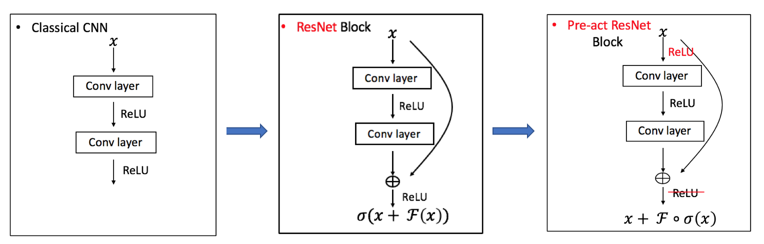
Figure 1: Comparison of classical CNN, ResNet and pre-act ResNet

Here we use the notation that $\sigma(x)={\rm ReLU}(x):=\max\{0,x\}$ as the standard ReLU activation function. For ResNet and pre-act ResNet with basic block, $\mathcal{F}(x)=A\ast\sigma\circ B\ast x$ where $A$ and $B$ are $3\times 3$ convolutions with multichannel, zero padding and stride one and “$\circ$” means composition. Our goal here is to investigate the interpretable mathematical model behind these models. To do that, let us first try to write these CNN models with specific mathematical formulas.

Pre-act ResNet

Different from the general researches by using diagram to identify these CNN architectures, we use some exact mathematical formula to write CNN models. One main component in the pre-act ResNet [14] without the last fully connected and soft-max layers, it can be written as in Algorithm 1.

Algorithm 1 $h=\text{pre-act ResNet}(f;J,\nu_{1},\cdots,\nu_{J})$

1:  Initialization: $r^{1,0}=f_{\rm in}(f)$.

2:  for $\ell=1:J$ do

3:     for $i=1:\nu_{\ell}$ do

4:        Basic Block:

$$r^{\ell,i}=r^{\ell,i-1}+A^{\ell,i}\ast\sigma\circ B^{\ell,i}\ast\sigma(r^{\ell,i-1}).$$ (2.1)

5:     end for

6:     Pooling(Restriction):

$$r^{\ell+1,0}=R_{\ell}^{\ell+1}\ast_{2}r^{\ell,\nu_{\ell}}+A^{\ell+1,0}\circ\sigma\circ B^{\ell+1,0}\ast_{2}\sigma(r^{\ell,\nu_{\ell}}).$$ (2.2)

7:  end for

8:  Final average pooling layer: $h=R_{\rm ave}(r^{L,\nu_{\ell}})$.

Here $f_{\rm in}(\cdot)$ may depend on different data set and problems such as $f_{\rm in}(f)=\sigma\circ\theta^{0}\ast f$ for CIFAR [21] and $f_{\rm in}(f)=R_{\rm max}\circ\sigma\circ\theta^{0}\ast f$ for ImageNet [3] as in [14]. In addition $r^{\ell,i}=r^{\ell,i-1}+A^{\ell,i}\ast\sigma\circ B^{\ell,i}\ast\sigma(r^{i-1})$ is often called the basic ResNet block. Here, $A^{\ell,i}$ with $i\geq 0$ and $B^{\ell,i}$ with $i\geq 1$ are general $3\times 3$ convolutions with zero padding and stride 1. In pooling block, $\ast_{2}$ means convolution with stride 2 and $B^{\ell,0}$ is taken as the $3\times 3$ kernel with same output channel dimension of $R_{\ell}^{\ell+1}$ which is taken as $1\times 1$ kernel and called as projection operator in [14]. During two consecutive pooling blocks, index $\ell$ means the fixed resolution or we $\ell$-th grid level as in multigrid methods. Finally, $R_{\rm ave}$ ($R_{\rm max}$) means average (max) pooling with different strides which is also dependent on datasets and problems.

ResNet

The original ResNet, developed earlier in [13], shares almost the same scheme with pre-act ResNet but with a different order of convolution and activation function. For ResNet model, these basic block and pooling are defined by:

$$r^{\ell,i} =\sigma\left(r^{\ell,i-1}+A^{\ell,i}\ast\sigma\circ B^{\ell,i}\ast r^{\ell,i-1}\right),$$ (2.3)

$$r^{\ell+1,0} =\sigma\left(R_{\ell}^{\ell+1}\ast_{2}r^{\ell,\nu_{\ell}}+A^{\ell+1,0}\ast\sigma\circ B^{\ell+1,0}\ast_{2}r^{\ell,\nu_{\ell}}\right),$$ (2.4)

for $i=1:\nu_{\ell}$.

3 Constrained Linear Data-feature Mapping

In this section, we will establish a new understanding of pre-act ResNet by involving the idea that the pre-act ResNet block is an iterative scheme for solving some hidden model in each grid. We adopt this assumption into these ResNet type models and get some modified models with a special parameter sharing scheme.

3.1 Constrained linear data-feature mapping and iterative methods

The main point here is the introduction of the so-called data and feature space for CNN, which is analogous to the function space and its duality in the theory of multigrid methods [40]. Namely, following [11] we introduce the next data-feature mapping model in every grid level follows:

$$A^{\ell}\ast u^{\ell}=f^{\ell},$$ (3.1)

where $f^{\ell}$ and $u^{\ell}$ belong to the data and feature space at $\ell$-th grid. We now make the following two important observations for this data-feature mapping:

• The mapping in (3.1) is linear, more specifically it is just a convolution with multichannel, zero padding and stride one as in pre-act ResNet.

• In each level, namely between two consecutive pooling, there is only one data-feature mapping, or we say that $A^{\ell}$ only depends on $\ell$, but not on number of layers.

We note that this the assumption that these linear data-feature mapping depend only on the grid level $\ell$ is motivated from a basic property of multigrid methods [39, 10, 40].

Besides (3.1), we introducing an important constrained condition in feature space that

$$u^{\ell,i}\geq 0.$$ (3.2)

The rationality of this constraint in feature space can be interpreted as follows. First of all, from the real neural system, the real neurons will only be active if the electric signal is greater than certain thresholding value. Namely, we can think that human brains can only see features with certain threshold. On the other hand, the “shift” invariant property of feature space in CNNs, namely, $u+a$ will not change the classification results. This means that $u+a$ should have the same classification result with $u$. That is to say, we may assume that $u\geq 0$ to reduce some redundancy of $u$.

Based on these assumptions above, what we need to do next is to solve the data-feature mapping equation in (3.1). We will adopt some classical iterative methods [39] in scientific computing to solve the system (3.1) and obtain that

$$u^{\ell,i}=u^{\ell,i-1}+B^{\ell,i}\ast(f^{\ell}-A^{\ell}\ast u^{\ell,i-1}),~{}i=1:\nu_{\ell},$$ (3.3)

where $u^{\ell}\approx u^{\ell,\nu_{\ell}}$. For more details about iterative methods in numerical analysis, we refer to [39, 9, 5]. To preserve (3.2), we naturally use the ReLU activation function $\sigma$ to modify (3.3) as follows

$$u^{\ell,i}=u^{\ell,i-1}+\sigma\circ B^{\ell,i}\ast\sigma(f^{\ell}-A^{\ell}\ast u^{\ell,i-1}),\quad i=1:\nu_{\ell}.$$ (3.4)

Because of the linearity of convolution in data-feature mapping, if we consider the residual $r^{\ell,j}=f^{\ell}-A^{\ell}\ast u^{\ell,j}$, (3.4) leads to the next iterative forms for residuals

$$r^{\ell,i}=r^{\ell,i-1}-A^{\ell}\ast\sigma\circ B^{\ell,i}\ast\sigma(r^{\ell,i-1}).$$ (3.5)

This is the same as (2.3) under the constraint $A^{\ell,i}=A^{\ell}$ in pre-act ResNet.

We summarize the above derivation in the following simple theorem.

Theorem 1.

Under the assumption that there is only one linear data-feature mapping in each grid $\ell$, i.e. $A^{\ell,i}=A^{\ell}$, the iterative form in feature space as in (3.3) is equivalent to (3.5) if $A^{\ell}$ is invertible where $r^{\ell,i}=f^{\ell}-A^{\ell}\ast u^{\ell,i}$.

3.2 Modified pre-act ResNet and ResNet

In this subsection we will propose some modified ResNet and pre-act ResNet models based on the assumption of the constrained linear data-feature mapping behind these models. While the scheme in (3.5) is closely related to the original pre-act ResNet,there is a major difference with an extra constraint that $A^{\ell,i}=A^{\ell}$. As a result, we obtain these next modified pre-act ResNet first as

Modified Pre-act ResNet (Pre-act ResNet-$A^{\ell}$-$B^{\ell,i}$)

$$r^{\ell,i}=r^{\ell,i-1}+A^{\ell}\ast\sigma\circ B^{\ell,i}\ast\sigma(r^{\ell,i-1}).$$ (3.6)

Here, we make a small modification of the sign before $A^{\ell}$ in formula since the linearity of convolution. As we discussed before, the modified pre-act ResNet model is derived from the constrained linear data-feature mapping by using a special iterative scheme. Although we cannot get these connections in ResNet directly, formally we can just make the modification from $A^{\ell,i}$ to $A^{\ell}$ into (2.1) to obtain the corresponding modified ResNet models as follows,

Modified ResNet (ResNet-$A^{\ell}$-$B^{\ell,i}$)

$$r^{\ell,i}=\sigma\left(r^{\ell,i-1}+A^{\ell}\ast\sigma\circ B^{\ell,i}\ast r^{\ell,i-1}\right).$$ (3.7)

A unified but simple diagram ignoring the activation functions for these modified pre-act ResNet and ResNet with this structure can be shown as in Figure 2.

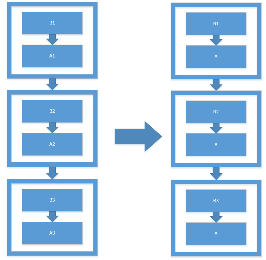
Figure 2: Diagram of modified (pre-act) ResNet basic blocks.

4 Linear versus nonlinear data-feature mapping

In this section, we will try to investigate the rationality for the constrained linear data-feature mapping. We will show that linear data-feature mapping model is adequate by comparing with some special nonlinear models on the data-feature mapping.

4.1 Nonlinear data-feature mapping and iterative methods

One of the most important assumptions above is that the data-feature mapping (3.1) could be a linear model and there should be only one model in each grid. To demonstrate that this linear model is adequate for image classification, we compare it with the following nonlinear data-feature mapping:

$$\mathcal{A}^{\ell}(u^{\ell})=f^{\ell},$$ (4.1)

where $\mathcal{A}^{\ell}$ can be chosen for some special nonlinear forms, such as $A^{\ell}\ast\sigma$, $\sigma\circ A^{\ell}\ast$, and $\sigma\circ A^{\ell}\ast\sigma$. Then we have the next iterative feature extraction scheme:

$$u^{\ell,i}=u^{\ell,i-1}+\mathcal{B}^{\ell,i}(f^{\ell}-\mathcal{A}^{\ell}(u^{\ell,i-1})),~{}i=1:\nu_{\ell},$$ (4.2)

where $\mathcal{B}^{\ell,i}$ can also take some special nonlinear forms. Here we note that, because of the nonlinearity of $\mathcal{A}^{\ell}$, we cannot got the iterative scheme about the residuals for (4.2). Namely, we can only do iteration in the feature space. Thus, we propose the next feature based ResNet (FB-ResNet) in Algorithm 2, which consists of the iteration of features as in (4.2) and a special pooling (4.4).

Algorithm 2 $u^{J,\ell_{J}}=\text{ FB-ResNet}(f;J,\nu_{1},\cdots,\nu_{J})$

1:  Initialization: $f^{1}=f_{\rm in}(f)$, $u^{1,0}=0$

2:  for $\ell=1:J$ do

3:     for $i=1:\nu_{\ell}$ do

4:        Feature extraction (smoothing):

$$u^{\ell,i}=u^{\ell,i-1}+\mathcal{B}^{\ell,i}\left({f^{\ell}-\mathcal{A}^{\ell}(u^{\ell,i-1})}\right).$$ (4.3)

5:     end for

6:     Pooling (interpolation and restriction):

$$u^{\ell+1,0} =\Pi_{\ell}^{\ell+1}\ast_{2}u^{\ell,\nu_{\ell}}$$ (4.4)

$$f^{\ell+1} =R^{\ell+1}_{\ell}\ast_{2}(f^{\ell}-\mathcal{A}^{\ell}(u^{\ell,\nu_{\ell}})+\mathcal{A}^{\ell+1}(u^{\ell+1,0}).$$

7:  end for

Here (4.4) are understood as different interpolation and restriction operators because of the difference of the feature and data space. However, in really implementation there are all implemented by $3\times 3$ convolution with stride 2 as $\Pi_{\ell}^{\ell+1}\ast_{2}$ and $R^{\ell+1}_{\ell}\ast_{2}$. We note that the idea to use the feature as the iterative unit is also proposed in MgNet [11]. More detailed discuss about the relation and comparison between typical pooling operation such as (2.2) and restriction in (4.4) could be found in Section 1 in the supplementary materials.

4.2 Numerical comparisons

To investigate the optimality of the linear assumption of $\mathcal{A}^{\ell}$, us first assume that we still keep the linearity assumption about $\mathcal{A}^{\ell}$ with the iterative method (4.2). Then we can have the next iterative scheme for residuals $r^{\ell,i}=f^{\ell}-\mathcal{A}^{\ell}(u^{\ell,i})$ as:

$$r^{\ell,i}=r^{\ell,i-1}-\mathcal{A}^{\ell}\mathcal{B}^{\ell,i}(r^{\ell,i-1}).$$ (4.5)

If we take the following specific settings: $\mathcal{A}^{\ell}(u)=A^{\ell}\ast u$ and $\mathcal{B}^{\ell,i}(r)=\sigma\circ B^{\ell,i}\ast\sigma(r)$. The iterative scheme for residuals will becomes

$$r^{\ell,i}=r^{\ell,i-1}-A^{\ell}\ast\sigma\circ B^{\ell,i}\ast\sigma(r^{\ell,i-1}),$$ (4.6)

which is exact the modified pre-act ResNet scheme as we discussed before.

Thus, we try some numerical experiments with “symmetric” forms for different linear or nonlinear forms for both $\mathcal{A}^{\ell}$ and $\mathcal{B}^{\ell,i}$ as:

$$K\ast,~{}K\ast\sigma,~{}\sigma\circ K\ast,~{}\text{and}~{}\sigma\circ K\ast\sigma,$$ (4.7)

where $K$ is a $3\times 3$ convolution kernel with multichannel, zero padding and stride one. These models can also be understood with the similar idea in pre-act ResNet, which are obtained by moving these activation functions and convolutions around in ResNet. In some sense, this is another important reason that why we propose the FB-ResNet as it is in feature space. Otherwise, it will be too close to the method in developing pre-act ResNet as in [14] if we still take its iterative scheme for residual form. The next table shows the numerical results with different combinations of linear or nonlinear schemes for $\mathcal{A}^{\ell}$ and $\mathcal{B}^{\ell,i}$.

Table 1: TOP-1 accuracy of models from Algorithm 2 with different linear or non-linear schemes of $\mathcal{A}$ and $\mathcal{B}$ on CIFAR10.

Schemes of $\mathcal{A}$ and $\mathcal{B}^{\ell,i}$	Accuracy
$\mathcal{A}^{\ell}=A^{\ell}\ast$,  $\mathcal{B}^{\ell,i}=B^{\ell,i}\ast$	70.96
$\mathcal{A}^{\ell}=A^{\ell}\ast$,  $\mathcal{B}^{\ell,i}=\sigma\circ B^{\ell,i}\ast$	92.82
$\mathcal{A}^{\ell}=A\ast$,  $\mathcal{B}^{\ell,i}=B^{\ell,i}\ast\sigma$	93.01
$\mathcal{A}^{\ell}=A^{\ell}\ast$,  $\mathcal{B}^{\ell,i}=\sigma\circ B^{\ell,i}\ast\sigma$	93.49
$\mathcal{A}^{\ell}=A^{\ell}\ast\sigma$,  $\mathcal{B}^{\ell,i}$ = $B^{\ell,i}\ast$	92.64
$\mathcal{A}^{\ell}=A^{\ell}\ast\sigma$,  $\mathcal{B}^{\ell,i}=\sigma\circ B^{\ell,i}\ast$	92.54
$\mathcal{A}^{\ell}=A^{\ell}\ast\sigma$,  $\mathcal{B}^{\ell,i}=B^{\ell,i}\ast\sigma$	93.46
$\mathcal{A}^{\ell}=A^{\ell}\ast\sigma$,  $\mathcal{B}^{\ell,i}=\sigma\circ B^{\ell,i}\ast\sigma$	93.15
$\mathcal{A}^{\ell}=\sigma\circ A^{\ell}\ast$,  $\mathcal{B}^{\ell,i}$ = $B^{\ell,i}\ast$	91.91
$\mathcal{A}^{\ell}=\sigma\circ A^{\ell}\ast$,  $\mathcal{B}^{\ell,i}=\sigma\circ B^{\ell,i}\ast$	92.14
$\mathcal{A}^{\ell}=\sigma\circ A^{\ell}\ast$,  $\mathcal{B}^{\ell,i}=B^{\ell,i}\ast\sigma$	93.37
$\mathcal{A}^{\ell}=\sigma\circ A^{\ell}\ast$,  $\mathcal{B}^{\ell,i}=\sigma\circ B^{\ell,i}\ast\sigma$	93.17
$\mathcal{A}^{\ell}=\sigma\circ A^{\ell}\ast\sigma$,  $\mathcal{B}^{\ell,i}$ = $B^{\ell,i}\ast$	92.70
$\mathcal{A}^{\ell}=\sigma\circ A^{\ell}\ast\sigma$,  $\mathcal{B}^{\ell,i}=\sigma\circ B^{\ell,i}\ast$	93.23
$\mathcal{A}^{\ell}=\sigma\circ A^{\ell}\ast\sigma$,  $\mathcal{B}^{\ell,i}=B^{\ell,i}\ast\sigma$	93.37
$\mathcal{A}^{\ell}=\sigma\circ A^{\ell}\ast\sigma$,  $\mathcal{B}^{\ell,i}=\sigma\circ B^{\ell,i}\ast\sigma$	93.40

From the results in Table 1, we show that the original assumption about the linearity of $\mathcal{A}^{\ell}$ and the special non-linear form of $\mathcal{B}^{\ell,i}$ is the most rational and accurate scheme which is also consistent with the theoretical concern and numerical results as in this paper.

5 Experiments

Our numerical experiments indicate that fixing the linear data-feature mapping in each grids only bring little negative or sometimes good effects than the standard ResNet and pre-act ResNet, which demonstrate the rational of the constrained data-feature mapping model.

5.1 Datasets, models and training details

Datasets

We evaluate our methods on the following widely used datasets: MNIST [25] , CIFAR datasets [21](CIFAR10, CIFAR100) and ImageNet [3]. We follow a typical or default way to split these datasets into training and validation data sets with standard data augmentation scheme which is widely used for these datasets [31, 13, 14, 17].

Models implementation

In our experiments, the structure of classical ResNet or pre-act ResNet models are implemented with the same structure as in the sample codes in PyTorch or Torchvision. As for our modified models, we implement them after some modifications of these standard codes. Following the strategy in [13, 14], we adopt Bath Normalization [18] but no Dropout [34].

Training details

We adopt the SGD training algorithm with momentum of $0.9$ and the weight initialization strategy as in [12]. We also adopt weight decay, which are $0.0001$ for ResNet18 type models and $0.001$ for ResNet34 type models. We take minibatch size to be 128, 128, 256 for MNIST, CIFAR and ImageNet, respectively. We start with a learning rate of 0.1, divide it by 10 every 30 epochs, and terminate training at 60 epochs for MNIST and 120 epochs for CIFAR. On ImageNet, we start with a learning rate of 0.1, divide it by 10 every 40 epochs, and terminate training at 120 epochs.

5.2 Classification accuracy on dataset for modified models

This modified pre-act ResNet can also be understood as a special parameter sharing form on $A^{\ell,i}$. With the similar idea, we want to prove that the linear model real makes sense not because of the redundancy of CNNs. Thus, we also put this parameter sharing scheme to $B^{\ell,i}$ or both $A^{\ell,i}$ and $B^{\ell,i}$ for pre-act ResNet.

Pre-acc ResNet-$A^{\ell,i}$-$B^{\ell}$:

$r^{\ell,i}=r^{\ell,i-1}+A^{\ell,i}\ast\sigma\circ B^{\ell}\ast\sigma(r^{\ell,i-1}),\quad i=1:\nu_{\ell}.$

Pre-acc ResNet-$A^{\ell}$-$B^{\ell}$:

$r^{\ell,i}=r^{\ell,i-1}+A^{\ell}\ast\sigma\circ B^{\ell}\ast\sigma(r^{\ell,i-1}),\quad i=1:\nu_{\ell}.$

The corresponding architectures for ResNet is defined in the same fashion. Because of the special role for $B^{\ell,0}$, we only share $B^{\ell,i}$ for $i=1:\nu_{\ell}$. For simplicity and consistency, we denote the classical ResNet and pre-act ResNet as ResNet-$A^{\ell,i}$-$B^{\ell,i}$ and pre-act ResNet-$A^{\ell,i}$-$B^{\ell,i}$.

Table 2: The TOP-1 accuracy and number of parameters of ResNet-18, pre-act ResNet-18 and their modified models on MNIST.

Model	Accuracy	# Parameters
ResNet18-$A^{\ell,i}$-$B^{\ell,i}$	99.56	11M
ResNet18-$A^{\ell}$-$B^{\ell,i}$	99.58	8.0M
pre-act ResNet18-$A^{\ell,i}$-$B^{\ell,i}$	99.61	11M
pre-act ResNet18-$A^{\ell}$-$B^{\ell,i}$	99.64	8.0M

Table 3: The TOP-1 accuracy and number of parameters for ResNet, pre-act ResNet and their variants of modified versions on CIFAR10 and CIFAR100.

Model	CIFAR10	CIFAR100	# Parameters
ResNet18-$A^{\ell,i}$-$B^{\ell,i}$	93.45	74.45	11M
ResNet18-$A^{\ell}$-$B^{\ell,i}$	93.54	74.46	8.1M
ResNet18-$A^{\ell,i}$-$B^{\ell}$	93.35	72.78	9.7M
ResNet18-$A^{\ell}$-$B^{\ell}$	93.32	72.56	6.6M
pre-act ResNet18-$A^{\ell,i}$-$B^{\ell,i}$	93.75	74.33	11M
pre-act ResNet18-$A^{\ell}$-$B^{\ell,i}$	93.83	74.51	8.1M
pre-act ResNet18-$A^{\ell,i}$-$B^{\ell}$	93.80	72.67	9.7M
pre-act ResNet18-$A^{\ell}$-$B^{\ell}$	93.45	72.81	6.6M
ResNet34-$A^{\ell,i}$-$B^{\ell,i}$	94.71	77.20	21M
ResNet34-$A^{\ell}$-$B^{\ell,i}$	94.84	77.24	13M
ResNet34-$A^{\ell,i}$-$B^{\ell}$	93.94	75.31	15M
ResNet34-$A^{\ell}$-$B^{\ell}$	93.79	74.79	6.7M
pre-act ResNet34-$A^{\ell,i}$-$B^{\ell,i}$	94.76	77.25	21M
pre-act ResNet34-$A^{\ell}$-$B^{\ell,i}$	94.84	77.40	13M
pre-act ResNet34-$A^{\ell,i}$-$B^{\ell}$	93.94	75.36	15M
pre-act ResNet34-$A^{\ell}$-$B^{\ell}$	93.75	75.82	6.7M

Table 4: The TOP-1 accuracy and number of parameters for ResNet, pre-act ResNet and their variants of modified versions on ImageNet.

Model	Accuracy	# Parameters
ResNet18-$A^{\ell,i}$-$B^{\ell,i}$	70.23	11.7M
ResNet18-$A^{\ell}$-$B^{\ell,i}$	69.45	8.6M
pre-act ResNet18-$A^{\ell,i}$-$B^{\ell,i}$	70.46	11.7M
pre-act ResNet18-$A^{\ell}$-$B^{\ell,i}$	69.78	8.6M

From these numerical results, we have the next two important observations: (1) The modified ResNet and pre-act ResNet models achieve almost the same accuracy to the original models on different datasets as shown in Tables 2, 3 and 4. (2) Only models with $A^{\ell}$ type can keep the accuracy, which is consistent with our analysis of the constrained linear data-mapping. Any models formally modified by changing $B^{\ell,i}$ to $B^{\ell}$ have lower accuracy, especially on CIFAR100. These observations indicate that constrained data-feature mapping together with the relevant iterative methods can provide mathematical insights of the ResNet and pre-act ResNet models.

6 Discussion and Conclusion

In this paper, we propose a constrained linear data-feature mapping model behind CNN models for image classification such as ResNet. Under this assumption, we carefully study the connections between the traditional iterative method with nonlinear constraint and the basic block scheme in pre-act ResNet model, and make an explanation for pre-act ResNet in a technical level. Comparing with other existing works that discuss the connection between dynamic systems and ResNet, the constrained data-feature mapping model goes beyond formal or qualitative comparisons and identifies key model components with much more details. Furthermore, we hope that how and why ResNet type models work can be mathematically understood in a similar fashion as for classical iterative methods in scientific computing which has a much more mature and better developed theory. Some numerical experiments are verified in this paper which indicate the rational and efficiency for the constrained learning data-feature mapping model.

We hope our attempt about the connection of CNNs and classical iterative methods can open a new door to the mathematical understanding, analysis and improvements of CNNs with some special structures. These results presented in this paper have demonstrated the great potential of this model from both theoretical and empirical viewpoints. Obviously many aspects of classical iterative methods with constraint should be further explored and expect to be much improved. For example, we are trying to establish the connection of DenseNet and the the so-called multi-step iterative methods in numerical linear algebra [9, 5].

Appendix

A Comparison between pooling block of ResNet and restriction in multigrid

So far, we investigate the basic iterative block for pre-act ResNet from the data-feature mapping perspective. We now try to involve the pooling block into this framework by introducing the multi-scale structure as in multigrid [39, 10]. We will now make comparison between the pooling block in pre-act ResNet with the standard restriction in multigrid for residual. Here, we first introduce the pooling block in modified pre-act ResNet as

$$\tilde{r}^{\ell+1,0}=\tilde{R}_{\ell}^{\ell+1}\ast_{2}r^{\ell,\nu_{\ell}}+\tilde{A}^{\ell+1}\ast\sigma\circ\tilde{B}^{\ell+1,0}\ast_{2}\sigma(r^{\ell,\nu_{\ell}}).$$ (6.1)

While, using the pooling of residual in multigrid, we have

$$r^{\ell+1,0}=R_{\ell}^{\ell+1}\ast_{2}(f^{\ell}-A^{\ell}(u^{\ell,\nu_{\ell}}))=R_{\ell}^{\ell+1}\ast_{2}r^{\ell,\nu_{\ell}}.$$ (6.2)

Take this into feature extraction, we have

$$r^{\ell+1,1}=r^{\ell+1,0}+A^{\ell+1}\ast\sigma\circ B^{\ell+1,1}\ast\sigma(r^{\ell+1,0}).$$ (6.3)

This means that

$$r^{\ell+1,1}=R_{\ell}^{\ell+1}\ast_{2}r^{\ell,\nu_{\ell}}+A^{\ell+1}\circ\sigma\circ B^{\ell+1,1}\ast\sigma(R_{\ell}^{\ell+1}\ast_{2}r^{\ell,\nu_{\ell}}).$$ (6.4)

By taking $\tilde{R}_{\ell}^{\ell+1}=R_{\ell}^{\ell+1}$ and $\tilde{A}^{\ell+1}=A^{\ell+1}$, we have

$$\tilde{r}^{\ell+1,0}=R_{\ell}^{\ell+1}\ast_{2}r^{\ell,\nu_{\ell}}+A^{\ell+1}\ast\sigma\circ\tilde{B}^{\ell+1,0}\ast_{2}\sigma(r^{\ell,\nu_{\ell}}).$$ (6.5)

Thus, the difference between $\tilde{r}^{\ell+1,0}$ and $r^{\ell+1,1}$ is noted in the difference of

$$\tilde{B}^{\ell+1,0}\ast_{2}\sigma(r^{\ell,\nu_{\ell}})~{}~{}\text{and}~{}~{}B^{\ell+1,1}\ast\sigma(R_{\ell}^{\ell+1}\ast_{2}r^{\ell,\nu_{\ell}}).$$ (6.6)

Here let us ignore the nonlinear activation and rewrite the convolution with stride $2$ as

$$\tilde{B}^{\ell+1,0}\ast_{2}r^{\ell,\nu_{\ell}}=S(\tilde{B}^{\ell+1,0}\ast r^{\ell,\nu_{\ell}}),$$ (6.7)

where $S$ means sub-sampling such as $[S(r)]_{i,j}=r_{2i-1,2j-1}$. Thus the difference in (6.6) becomes

$$S(\tilde{B}^{\ell+1,0}\ast r^{\ell,\nu_{\ell}})~{}\text{and}~{}B^{\ell+1,1}\ast R_{\ell}^{\ell+1}\ast S(r^{\ell,\nu_{\ell}}),$$ (6.8)

because of the fact that $R_{\ell}^{\ell+1}$ chooses $1\times 1$ kernel in pre-act ResNet. Let use consider that $r^{\ell,\nu_{\ell}}\in\mathbb{R}^{n_{\ell}\times n_{\ell}\times 1}$ and $[r^{\ell,\nu_{\ell}}]_{i,j}=0$ expect for $[r^{\ell,\nu_{\ell}}]_{2,2}=1$, then $S(r^{\ell,\nu_{\ell}})={\bm{0}}\in\mathbb{R}^{\frac{n_{\ell}}{2}\times\frac{n_{\ell}}{2}\times 1}$. However, we may learn some special $\tilde{B}^{\ell+1,0}$ such that $S(\tilde{B}^{\ell+1,0}\ast r^{\ell,\nu_{\ell}})\neq\bm{0}$ which can capture the one pixel feature. From this point of view, we may say that the pooling block (6.1) in pre-act ResNet makes sense to prevent loosing of small scale information. Thus, we will choose the pooling block in (6.1) to be the pooling block of modified ResNet ,pre-act ResNet or other models without special statements.

References

- [1] B. Chang, L. Meng, E. Haber, F. Tung, and D. Begert. Multi-level residual networks from dynamical systems view. arXiv preprint arXiv:1710.10348, 2017.
- [2] T. Q. Chen, Y. Rubanova, J. Bettencourt, and D. K. Duvenaud. Neural ordinary differential equations. In Advances in neural information processing systems, pages 6571–6583, 2018.
- [3] J. Deng, W. Dong, R. Socher, L.-J. Li, K. Li, and L. Fei-Fei. Imagenet: A large-scale hierarchical image database. In 2009 IEEE conference on computer vision and pattern recognition, pages 248–255. Ieee, 2009.
- [4] W. E. A proposal on machine learning via dynamical systems. Communications in Mathematics and Statistics, 5(1):1–11, 2017.
- [5] G. H. Golub and C. F. Van Loan. Matrix computations, volume 3. JHU press, 2012.
- [6] A. N. Gomez, M. Ren, R. Urtasun, and R. B. Grosse. The reversible residual network: Backpropagation without storing activations. In Advances in Neural Information Processing Systems, pages 2214–2224, 2017.
- [7] K. Gregor and Y. LeCun. Learning fast approximations of sparse coding. In Proceedings of the 27th International Conference on International Conference on Machine Learning, pages 399–406. Omnipress, 2010.
- [8] E. Haber, L. Ruthotto, and E. Holtham. Learning across scales-a multiscale method for convolution neural networks. arXiv preprint arXiv:1703.02009, 2017.
- [9] W. Hackbusch. Iterative solution of large sparse systems of equations, volume 95. Springer, 1994.
- [10] W. Hackbusch. Multi-grid methods and applications, volume 4. Springer Science & Business Media, 2013.
- [11] J. He and J. Xu. Mgnet: A unified framework of multigrid and convolutional neural network. Science China Mathematics, pages 1–24, 2019.
- [12] K. He, X. Zhang, S. Ren, and J. Sun. Delving deep into rectifiers: Surpassing human-level performance on imagenet classification. In Proceedings of the IEEE international conference on computer vision, pages 1026–1034, 2015.
- [13] K. He, X. Zhang, S. Ren, and J. Sun. Deep residual learning for image recognition. In Proceedings of the IEEE Conference on Computer Vision and Pattern Recognition, pages 770–778, 2016.
- [14] K. He, X. Zhang, S. Ren, and J. Sun. Identity mappings in deep residual networks. In European Conference on Computer Vision, pages 630–645. Springer, 2016.
- [15] U. Helmke and J. B. Moore. Optimization and dynamical systems. Springer Science & Business Media, 2012.
- [16] J.-T. Hsieh, S. Zhao, S. Eismann, L. Mirabella, and S. Ermon. Learning neural pde solvers with convergence guarantees. ICLR 2019, 2018.
- [17] G. Huang, Z. Liu, L. Van Der Maaten, and K. Q. Weinberger. Densely connected convolutional networks. In CVPR, volume 1, page 3, 2017.
- [18] S. Ioffe and C. Szegedy. Batch normalization: Accelerating deep network training by reducing internal covariate shift. arXiv preprint arXiv:1502.03167, 2015.
- [19] A. Katrutsa, T. Daulbaev, and I. Oseledets. Deep multigrid: learning prolongation and restriction matrices. arXiv preprint arXiv:1711.03825, 2017.
- [20] T.-W. Ke, M. Maire, and X. Y. Stella. Multigrid neural architectures. arXiv preprint arXiv:1611.07661, 2016.
- [21] A. Krizhevsky and G. Hinton. Learning multiple layers of features from tiny images. Technical report, Citeseer, 2009.
- [22] A. Krizhevsky, I. Sutskever, and G. E. Hinton. Imagenet classification with deep convolutional neural networks. In International Conference on Neural Information Processing Systems, pages 1097–1105, 2012.
- [23] G. Larsson, M. Maire, and G. Shakhnarovich. Fractalnet: Ultra-deep neural networks without residuals. arXiv preprint arXiv:1605.07648, 2016.
- [24] Y. LeCun, Y. Bengio, and G. Hinton. Deep learning. nature, 521(7553):436, 2015.
- [25] Y. LeCun, L. Bottou, Y. Bengio, and P. Haffner. Gradient-based learning applied to document recognition. Proceedings of the IEEE, 86(11):2278–2324, 1998.
- [26] H. Li, Y. Yang, D. Chen, and Z. Lin. Optimization algorithm inspired deep neural network structure design. arXiv preprint arXiv:1810.01638, 2018.
- [27] Z. Li and Z. Shi. A flow model of neural networks. arXiv preprint arXiv:1708.06257v2, 2017.
- [28] Y. Lu, A. Zhong, Q. Li, and B. Dong. Beyond finite layer neural networks: Bridging deep architectures and numerical differential equations. In Proceedings of the 35th International Conference on Machine Learning, volume 80. PMLR, 2018.
- [29] F. Milletari, N. Navab, and S. A. Ahmadi. V-net: Fully convolutional neural networks for volumetric medical image segmentation. In 2016 Fourth International Conference on 3D Vision (3DV), pages 565–571, Oct 2016.
- [30] O. Ronneberger, P. Fischer, and T. Brox. U-net: Convolutional networks for biomedical image segmentation. In International Conference on Medical Image Computing and Computer-Assisted Intervention, pages 234–241. Springer, 2015.
- [31] P. Sermanet, S. Chintala, and Y. LeCun. Convolutional neural networks applied to house numbers digit classification. In 2012 21st International Conference on Pattern Recognition (ICPR 2012), pages 3288–3291. IEEE, 2012.
- [32] K. Simonyan and A. Zisserman. Very deep convolutional networks for large-scale image recognition. Computer Science, 2014.
- [33] S. Sonoda and N. Murata. Double continuum limit of deep neural networks. In ICML Workshop Principled Approaches to Deep Learning, 2017.
- [34] N. Srivastava, G. Hinton, A. Krizhevsky, I. Sutskever, and R. Salakhutdinov. Dropout: a simple way to prevent neural networks from overfitting. The journal of machine learning research, 15(1):1929–1958, 2014.
- [35] J. Sun, H. Li, Z. Xu, et al. Deep admm-net for compressive sensing mri. In Advances in neural information processing systems, pages 10–18, 2016.
- [36] C. Szegedy, S. Ioffe, V. Vanhoucke, and A. A. Alemi. Inception-v4, inception-resnet and the impact of residual connections on learning. In Thirty-First AAAI Conference on Artificial Intelligence, 2017.
- [37] C. Szegedy, W. Liu, Y. Jia, P. Sermanet, S. Reed, D. Anguelov, D. Erhan, V. Vanhoucke, and A. Rabinovich. Going deeper with convolutions. In Proceedings of the IEEE conference on computer vision and pattern recognition, pages 1–9, 2015.
- [38] S. Xie, R. Girshick, P. Dollár, Z. Tu, and K. He. Aggregated residual transformations for deep neural networks. In Computer Vision and Pattern Recognition (CVPR), 2017 IEEE Conference on, pages 5987–5995. IEEE, 2017.
- [39] J. Xu. Iterative methods by space decomposition and subspace correction. SIAM Review, 34(4):581–613, 1992.
- [40] J. Xu and L. Zikatanov. Algebraic multigrid methods. Acta Numerica, 26:591–721, 2017.
- [41] S. Zagoruyko and N. Komodakis. Wide residual networks. In British Machine Vision Conference, pages 87.1–87.12, 2016.
- [42] L. Zhang, Z. Tan, J. Song, J. Chen, C. Bao, and K. Ma. Scan: A scalable neural networks framework towards compact and efficient models. arXiv preprint arXiv:1906.03951, 2019.
- [43] X. Zhang, Z. Li, C. C. Loy, and D. Lin. Polynet: A pursuit of structural diversity in very deep networks. In Computer Vision and Pattern Recognition (CVPR), 2017 IEEE Conference on, pages 3900–3908. IEEE, 2017.