Visualizing Point Cloud Classifiers by Curvature Smoothing
Abstract
Recently, several networks that operate directly on point clouds have been proposed. There is significant utility in understanding their mechanisms to classify point clouds, which can potentially help diagnosing these networks and designing better architectures. In this paper, we propose a novel approach to visualize features important to the point cloud classifiers. Our approach is based on smoothing curved areas on a point cloud. After prominent features were smoothed, the resulting point cloud can be evaluated on the network to assess whether the feature is important to the classifier. A technical contribution of the paper is an approximated curvature smoothing algorithm, which can smoothly transition from the original point cloud to one of constant curvature, such as a uniform sphere. Based on the smoothing algorithm, we propose PCI-GOS (Point Cloud Integrated-Gradients Optimized Saliency), a visualization technique that can automatically find the minimal saliency map that covers the most important features on a shape. Experiment results revealed insights into different point cloud classifiers. The code is available at https://github.com/arthurhero/PC-IGOS 111This work was done while Zhongang Qi was a Postdoctoral Scholar at Oregon State University
1 Introduction
Recently, direct deep learning on unstructured 3-D point clouds has gained significant interest. Many interesting point cloud networks have been proposed. PointNet++ [20] utilizes max-pooling followed by multi-layer perceptron. PointConv [30] realizes a convolution operation on point clouds efficiently. Other works such as [29, 25, 32, 3, 14, 8, 27] all have their own merits. As with 2-D image classifiers, we are curious about what these models have actually learned. Such explanations would help us gain more insights, diagnose the networks, and potentially design better network structures and data augmentation pipelines.
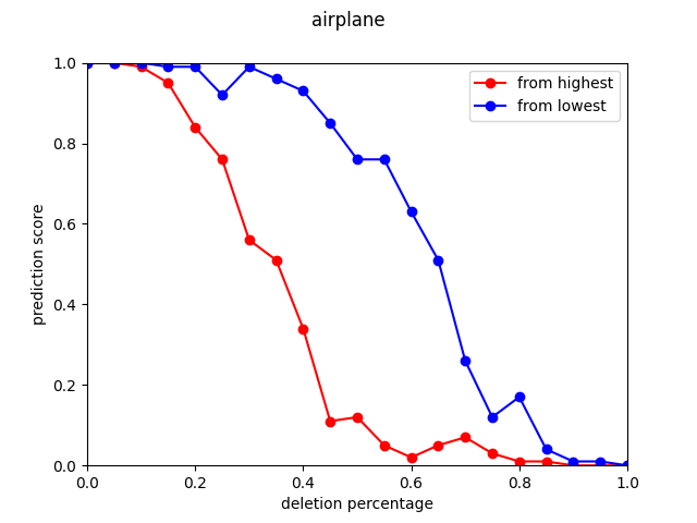
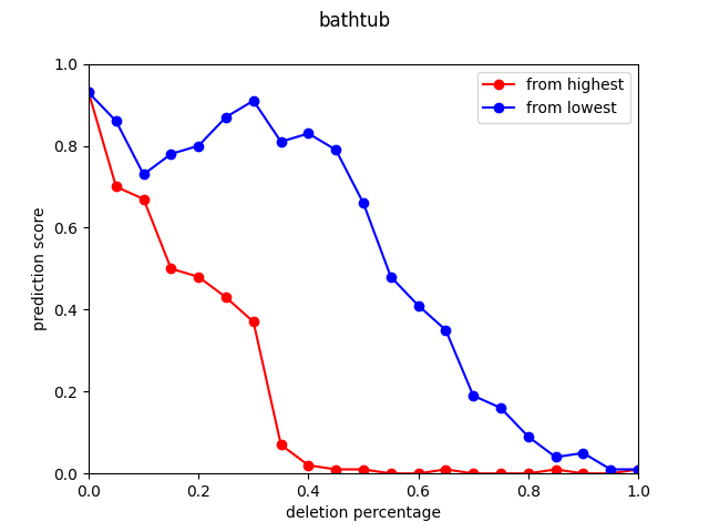
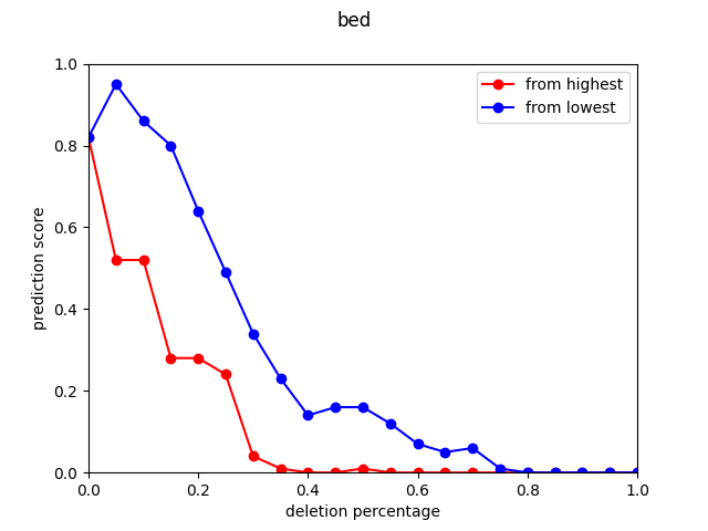
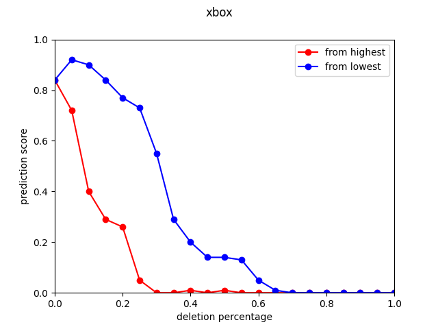
In this work, we are interested in looking for the most important features on a shape for the classifiers. Following the deletion and insertion metric proposed by [19], we should expect the predicted score to drop quickly when we “cover up” those important features, and to rise quickly when we gradually “reveal” only those important features. We want to design an algorithm that can automatically learn the minimal saliency map as in [9].
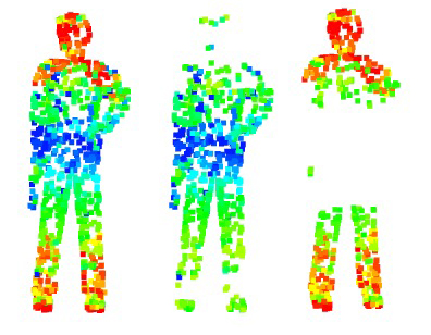
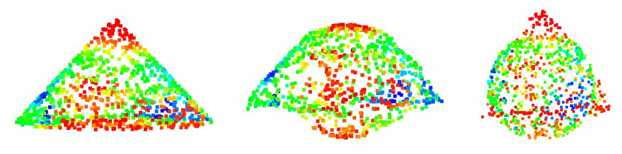
In order to apply a saliency map on a shape, we need an operator that can gradually “cover up” and “reveal” parts of a point cloud. For 2-D images we can simply apply different levels of Gaussian blur to the pixels. However in 3-D, no matter how we move the points, they will always be part of the point cloud, and thus contributing to the underlying shape. With the key observation that sharp features like edges and corners on a shape are reflected by abnormal curvatures on the underlying surface, we propose a novel, diffusion-based smoothing algorithm that can gradually smooth out curvatures on a point cloud. For instance, if the underlying surface is closed, then our algorithm will gradually morph the shape into a sphere.
With the smoothing method, we propose PCI-GOS (“point-cloud I-GOS”), a 3-D heatmap visualization algorithm. This extends the I-GOS algorithm [21] on 2D images to generate a saliency map that highlights points which are important for classifiers. We experiment our approach on PointConv [30], a state-of-the-art point cloud network. We compare our results on the ModelNet40 dataset with several baselines including Zheng et al. [34], a gradient-based visualization technique optimized for direct point deletion.
2 Related Work
Classifier visualization Using heatmaps to visualize networks has attracted much research effort these years. There are two main categories of approaches: gradient-based and perturbation-based. Gradient-based approaches utilizes the gradients of the output score w.r.t. the input as the standard of measuring input contribution [23, 33, 24, 4, 22, 26]. Perturbation-based methods, on the other hand, perturb the input and examine which parts of the input have the largest influence on the output. Object detectors in CNNs [35], Real Time Image Saliency [6], Meaningful Perturbation [9], RISE [19] and I-GOS [21] belong to this family.
As far as we know, [34] is the only prior work we know that attempts to visualize point cloud networks. [34] uses a gradient-based approach and calculates the gradients of the output score with respect to the straight line from median to the input points and regards those gradients as saliency.
3-D shape morphology There has been active research in smoothing and fairing 3-D structures. For mesh smoothing, [28] has proposed a method based on diffusion, and proved it to serve as a low-pass filter and is anti-shrinkage. However, as [7] pointed out, this diffusion method is flawed due to its unrealistic assumption about meshes. [7] proposed a scheme based on curvature flow, where a local “curvature normal” is computed at each vertex and the diffusion is based on it. Meshes are easier to smooth than point clouds because they provide readily estimated planes that can be used to compute curvature. Noise-removal schemes that directly operate on point clouds were proposed in [1] and [18]. Most of these methods are based on moving least-squares [13] with local plane/surface fitting. However, the goals of these approaches are mainly removing noises, rather than gradually morphing the shape to one with constant curvature as in our goal.
3 Methods
Throughout this paper we work on a point cloud with points, denoted as , where is a 3-tuple of coordinates. Denote a neighborhood of as and as the size of the neighborhood. Let represent the operator taking a vector and making it a diagonal matrix, be the identity matrix, and be the vector of all s.
3.1 Smoothing Point Clouds
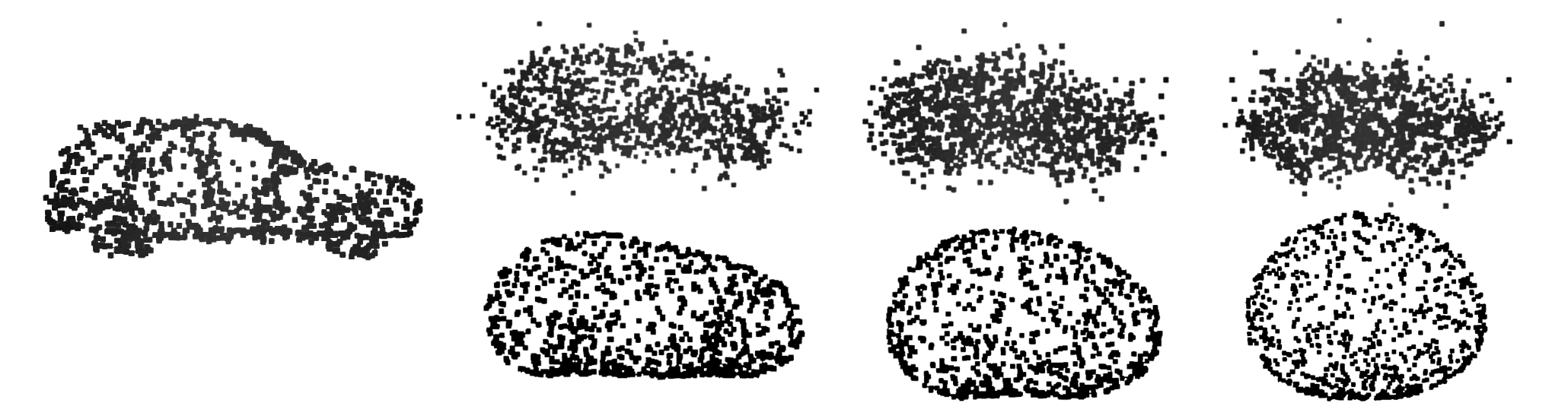
Our goal is to smoothly morph a point cloud into a feature-less shape. We regard “curvature” on the surface as features here, since edges and corners are all areas of large curvatures on the surface that are distinct from their surroundings. Hence, we want the curvature on the entire point cloud to be constant or has little variance. Assuming the underlying manifold is closed, this goal is equivalent to morphing the shape into a sphere.
3.1.1 Taubin Smoothing
Our idea is inspired by Taubin smoothing [28], a classical technique for meshes. In Taubin smoothing, the local Laplacian at a vertex is linearly approximated using the umbrella operator:
| (1) |
This approximation assumes unit-length edges and equal angles between two adjacent edges around a vertex [7]. has a matrix form where is the Laplacian matrix, assuming is the -nearest neighbor graph adjacency matrix in and is the diagonal degree matrix of each point (here means the matrix multiplication between and an all-one matrix. has constant s on its diagonal). Each vertex is then updated using the following scheme,
| (2) |
where and . The first equation in Eq.(2) refers to a diffusion operator equivalent to , so that once this operation is carried out multiple times, most of the eigenvalues of become close to zero and henceforth the points become more evenly distributed. Furthermore, [28] proposed to add a step to prevent shrinkage, so that the volume enclosed by the underlying manifold does not decrease. An intuition behind Taubin smoothing is that the first equation in Eq. (2) attenuates the high frequencies and the second one magnifies the remaining low frequencies.

3.1.2 Our algorithm
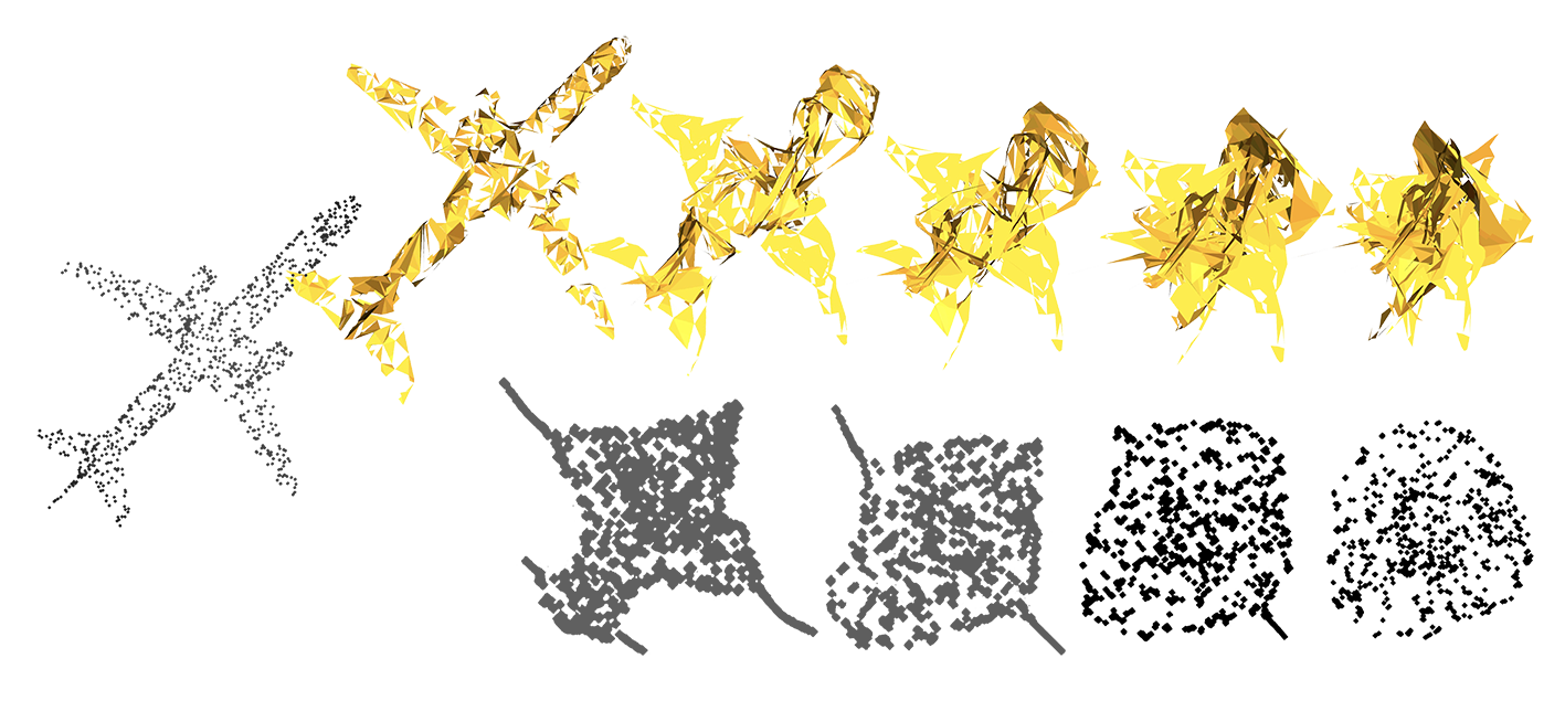
Based on the above diffusion formulation and with suitable parameter choices, Taubin smoothing should be able to smooth using any self-adjoint compact operator beyond the Laplacian operator [36]. [7] as an example smooths on the curvature normal operator on meshes. In this paper, we approximate the mean curvature at a point by calculating its distance to a plane locally fitted to its neighborhood. Fitting such a plane allows us to be more robust to noisy input point clouds (Fig. 9). Afterwards, we gradually filter out high frequency changes in curvature on the underlying surface of the point cloud. If the underlying shape is a closed manifold, our algorithm will be able to smooth it approximately into a sphere, where curvature is constant everywhere.
To fit a local plane for each point , we minimize the least-squares error:
| (3) |
Let denote the position of after being projected onto (i.e. ). Then is the vector pointing from the point to the plane . Note that the direction of is just the surface normal at . However, we hold that the distance to the plane is an approximation to the mean curvature, and coincides with the curvature under some simplifying assumption.
Theorem 1.
Let be a point in point cloud. Let be the plane fitted to the neighbors of . Let be the projection of on . Assuming ’s neighbors distribute evenly and densely on a ring surrounding , then the curvature normal at can be approximated by the expression , where is the distance from to any of its neighbor.
See the supplementary material for the proof.
With that result, we can accommodate the smoothing algorithm from [28] as follows:
| (4) |
where , and refers to the projection of on a new plane fitted for . Thus instead of moving the point toward the mean of its neighbors, we move it directly toward the locally fitted plane. We call the first equation in Eq. 4 the “erosion” round, and the second one the “dilation” round.
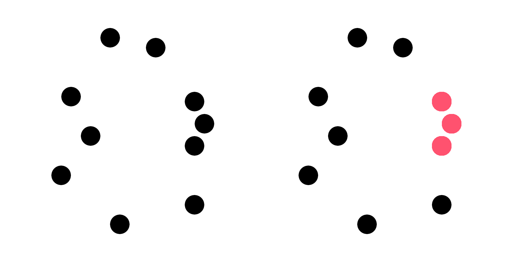
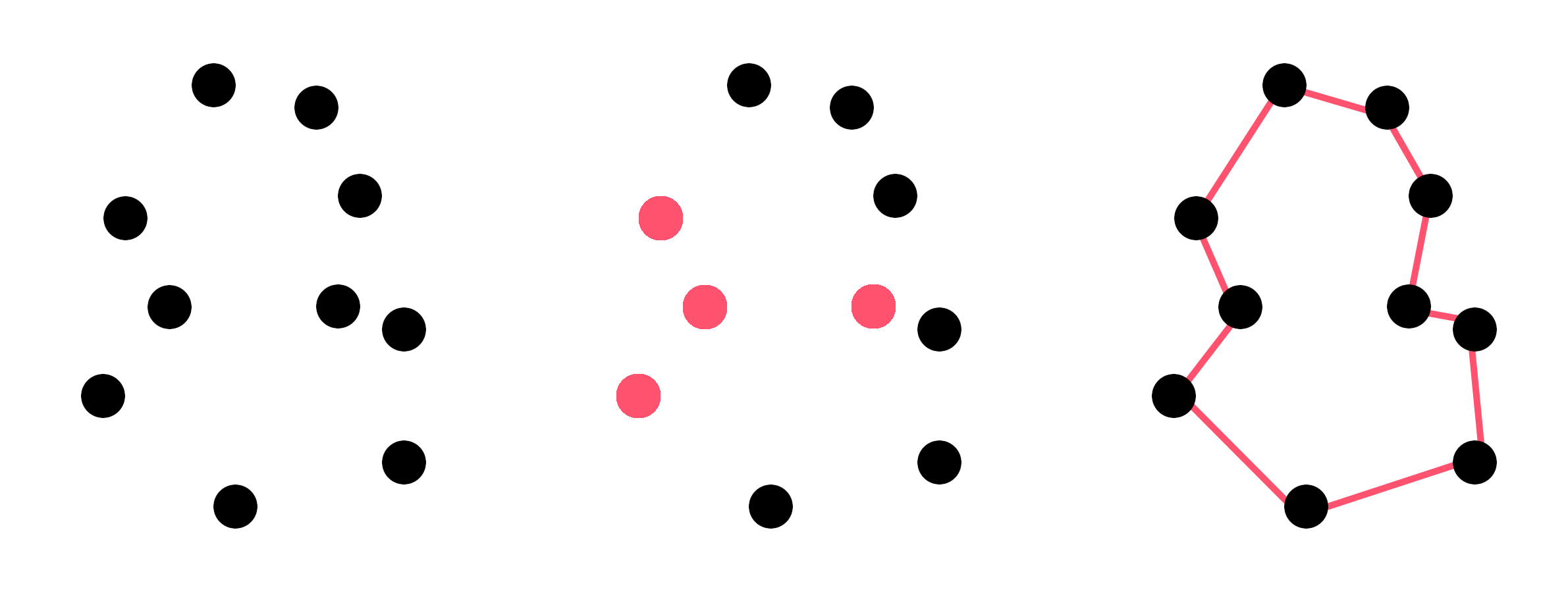
To deal with degenerate cases where the point cloud is already on a plane, we further extend the algorithm to a 2-D case (Fig. 5). Here the goal is to filter out high frequency changes in curvature on the boundary, transforming the plane to a disk. In this case, assuming all the neighborhood points are on the plane, we fit a line for by minimizing the least-squares error:
| (5) |
where each is the projection of to the plane . Let be the projection of on line . We update in the same fashion as in the 3-D case:
| (6) |
Denote the final 2D coordinates as , we convert it back to 3-D by calculating . In reality, due to noises, many points are not exactly on a plane. We project them to their local planes first, and then calculate the -coordinates from their projected location . Note that we still shift the point from its original location , not its projected location . In actual implementation, the 2-D version is used together with the 3-D version and is always run first. For example, in an “erosion” round, we run the first equation in Eq. (6), then the first equation in Eq. (4); in a “dilation” round, we run the second equation in Eq. (6), then the second equation in Eq. (4). Empirically this seems to generalize well on both planar and non-planar surfaces, we believe the reason is that on non-planar surfaces the line fitting usually falls close to the point itself, hence the planar version hardly moves any point at all. By utilizing both of them at every iteration, we avoid introducing an extra threshold to decide whether a neighborhood is on a plane.
3.2 Visualizing Point Cloud Classifiers
Our goal is to find the most important points that decide the output of a classifier. Following the idea of “mask” from [9], we achieve this goal by finding such a mask that the classification score is minimized when the mask is applied to the point cloud, and the score is maximized when the reverse of the mask is applied. Inspired by [26] and [21], we use an integrated loss to train our mask.
Let mask be of the same size as the point cloud , initialized with all zeros. Mask values are always between , where means no smoothing and means fully smoothing. Let our baseline point cloud be the fully smoothed point cloud (e.g. sphere) and let our baseline mask be , so that when applied to the shape, the shape becomes . The idea of an integrated mask is that we gradually morph to , which is a global minimum for the classification score loss, and collect the classification score loss along the path:
| (7) |
and
| (8) |
where represents the classifier on the class , denotes the reverse of the mask and represents the action of applying the mask to the point cloud. indicates the classification score should plunge as crucial features are gradually deleted ( to ) and indicates the classification score should increase significantly as crucial features are gradually inserted. The benefit of integrated gradients is that they are more likely pointing to a global optimum for the unconstrained problem of only minimizing the classification loss of a single mask, so that the optimization can evade local optima and achieve better performance. In practice, we approximate the integration process in the above equations by dividing it into 20 steps and average through the 20 losses.
However, with classification loss only, the algorithm might as well return the baseline mask . In order to identify the most important set of points, we must constrain the sum of mask values by using an loss .
Altogether, our mask is trained using the following losses
| (9) |
One difficulty of this algorithm is how to implement as a differentiable masking operation. In 2-D images, we can simply use a weighted (by ) average of the actual pixel value and the baseline pixel value. However, in point clouds, if we directly push a point toward its corresponding baseline position, undesirable (out-of-distribution) sharp structure might appear.
Ideally, we want to run more smoothing iterations on points with higher mask value. Unfortunately, the smoothing process is not parametrized by mask values.
In practice, we construct a differentiable by precomputing 10 intermediate shapes with increasing level of smoothness. Since the smoothing method we introduced is iterative, we simply run the algorithm for iterations and capture the shape after each iterations. We approximate the ideal mask smoothing operation by combining the 10 shapes:
| (10) |
where is a point with a mask value , refers to the -th point cloud in our sequence of precomputed smoothed shapes ( refers to and refers to the original shape), and refers to the position of the -th point in the -th point cloud. Here, we are using a Gaussian kernel to assign weights to each level of the masks. The closer and , the higher the weight. For example, when the mask value at is nearly transparent, will be low, and thus masks with lower smoothing level will gain greater weights. After obtaining the masked shape, we apply the point cloud classifier to get the classification score for the losses, and then calculate the gradients.
Under our algorithm, the mask converges quickly (we typically only need 30 optimization steps for each shape), and the resulting masks only make small changes to the original point clouds with a large impact on the prediction score, and are interpretable by human (as shown in Fig. 3). Finally, we output the mask as our saliency map.
4 Experiments
We have conducted two types of experiments. First, we compare our smoothing algorithm against several baselines to validate its smoothing capability. Second, we visualize point cloud classifiers using PCI-GOS, compared it with baselines as well as another visualization technique proposed by [34], and performed several ablation studies. All experiments are conducted on the test split of the ModelNet40 dataset, with the classifier trained on the training split. Each shape contains 1024 randomly sampled points, and only location information. Parameters of our smoothing algorithm are: , grows from 20 to 60. We run 80 iterations on each shape (one iteration one “erosion” one “dilation”).
4.1 Point cloud smoothing
Since there were few prior work that aim at morphing point clouds into spheres, we compare against several other plausible baselines. First note that directly applying Gaussian blur to point coordinates is not a valid baseline, because Gaussian blur tends to smooth the coordinate values, which results in pushing neighboring points to all have the same coordinates, leading to a skeleton effect. We compare against three baselines:
Meshing, then smoothing. This idea converts the point cloud to a mesh and then applies mesh-based smoothing techniques such as [7] to the result. For our goals, we chose [17] as an algorithm that does not change the number of points and maintains a 1-1 correspondence with the original point cloud. Due to the noisiness and sparsity of the point cloud, the meshing result is often not ideal.
Directly applying mesh smoothing techniques to points. Instead of explicit meshing, we construct an implicit mesh by assuming a point is connected to all its neighbors. Then, we directly apply mesh smoothing techniques to the point cloud. However, the uneven distribution of points in a point cloud quite often distorts the result.
Fitting a quadratic surface. We fit a quadratic surface to the local neighborhood instead of a plane. A quadratic surface allows analytic computation of the curvature, which is in principle a better approximation than the plane. We implemented the closed-form quadratic fitting algorithm following [11]. However, quadratic surfaces have a large degree of freedom and thus even a tiny noise can render an overfitting quadratic type or direction.
| Smooth level | 1 | 2 | 3 | 4 | 5 | 6 | 7 | 8 | 9 | 10 | |
|---|---|---|---|---|---|---|---|---|---|---|---|
| Mesh | CSD | 0.10 | 0.10 | 0.11 | 0.12 | 0.13 | 0.14 | 0.16 | 0.17 | 0.19 | 0.20 |
| MR | 0.82 | 0.82 | 0.82 | 0.82 | 0.82 | 0.83 | 0.86 | 0.85 | 0.83 | 0.83 | |
| DDS | 0.40 | 0.67 | 0.62 | 0.63 | 0.60 | 0.58 | 0.48 | 0.38 | 0.40 | 0.30 | |
| Taubin | CSD | 0.10 | 0.11 | 0.11 | 0.11 | 0.11 | 0.11 | 0.10 | 0.10 | 0.09 | 0.09 |
| MR | 0.83 | 0.84 | 0.83 | 0.87 | 0.88 | 0.86 | 0.86 | 0.86 | 0.75 | 0.73 | |
| DDS | 0.90 | 0.92 | 0.74 | 0.87 | 0.83 | 0.81 | 0.69 | 0.74 | 0.43 | 0.66 | |
| Quad | CSD | 0.11 | 0.12 | 0.12 | 0.12 | 0.12 | 0.12 | 0.13 | 0.13 | 0.13 | 0.13 |
| MR | 0.79 | 0.80 | 0.81 | 0.81 | 0.83 | 0.83 | 0.83 | 0.84 | 0.83 | 0.83 | |
| DDS | 0.76 | 0.83 | 0.84 | 0.89 | 0.82 | 0.89 | 0.92 | 0.92 | 0.88 | 0.94 | |
| Ours | CSD | 0.08 | 0.07 | 0.07 | 0.06 | 0.06 | 0.06 | 0.06 | 0.06 | 0.06 | 0.05 |
| MR | 0.85 | 0.87 | 0.88 | 0.89 | 0.91 | 0.92 | 0.94 | 0.94 | 0.95 | 0.95 | |
| DDS | 0.60 | 0.75 | 0.68 | 0.72 | 0.64 | 0.66 | 0.59 | 0.60 | 0.56 | 0.58 | |
| mask-only | ig-only | Zheng et al. | Ours | Zheng et al.[34] | Ours | |
|---|---|---|---|---|---|---|
| Curvature Del./Ins. | Point Del./Ins. | |||||
| Deletion | 0.2514 | 0.2812 | 0.2597 | 0.2214 | 0.2793 | 0.4073 |
| Insertion | 0.2917 | 0.3970 | 0.4219 | 0.4502 | 0.4976 | 0.5215 |
| w/o | w/o | msize=1024 | full | |
|---|---|---|---|---|
| Deletion | 0.2226 | 0.1965 | 0.2463 | 0.2214 |
| Insertion | 0.4419 | 0.3610 | 0.4109 | 0.4502 |
For a quantitative comparison against these baselines, we propose three metrics to evaluate our smoothing algorithm: curvature standard deviation (CSD), min-max ratio (MR) and density distribution similarity (DDS). The first two ensure that the final shape is feature-less as desired, and the last one ensures that the morphing process does not bring abrupt changes to the point cloud. Please refer to supplementary materials for more explanation about these metrics. Ten intermediate point clouds with increasing level of blurriness are sampled.
From the experiment results, all baseline algorithms fail to eliminate large curvatures on the surface. All of them fail to improve MR at all, which means the final shape is not sphere-like as desired. Only our algorithm succeeds in both removing features from the surface and keeping the morphing process smooth.
4.2 Classifier visualization
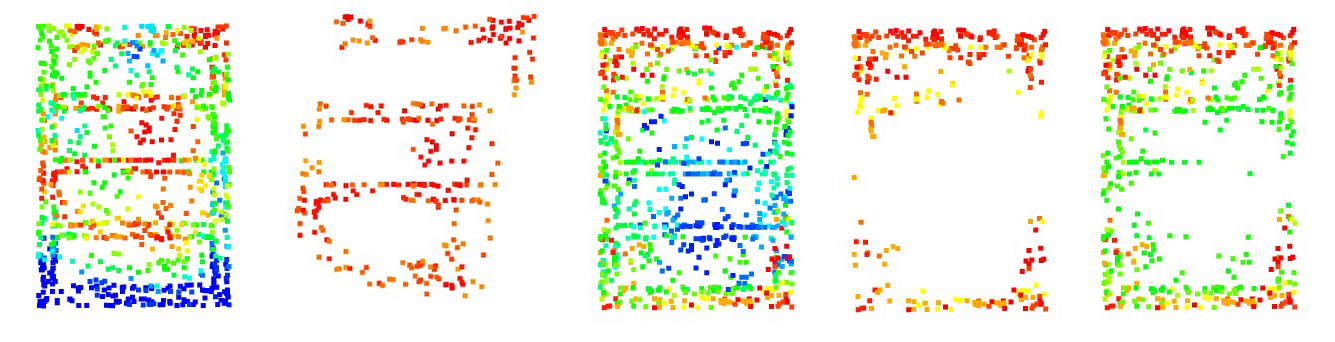
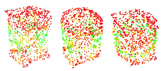
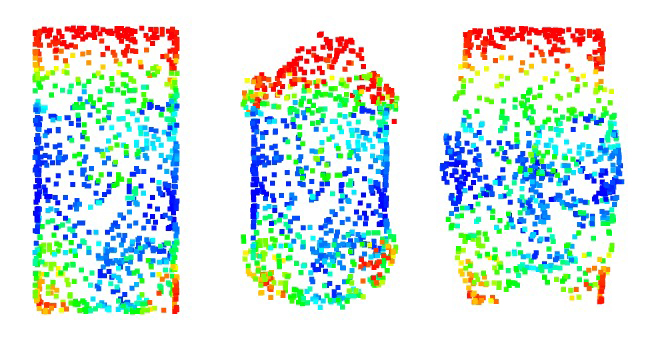
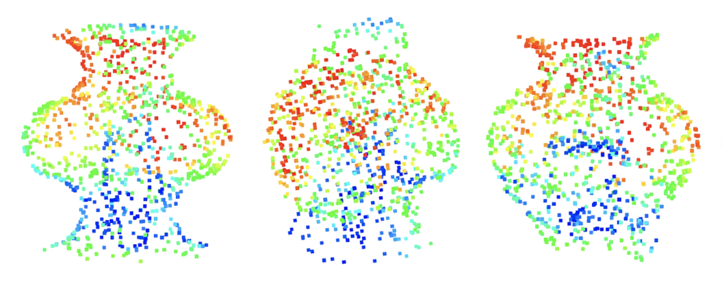
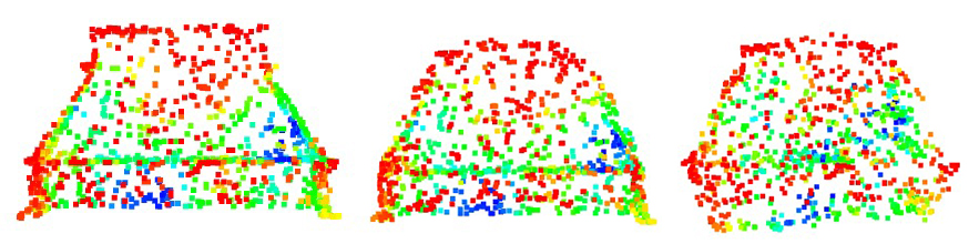
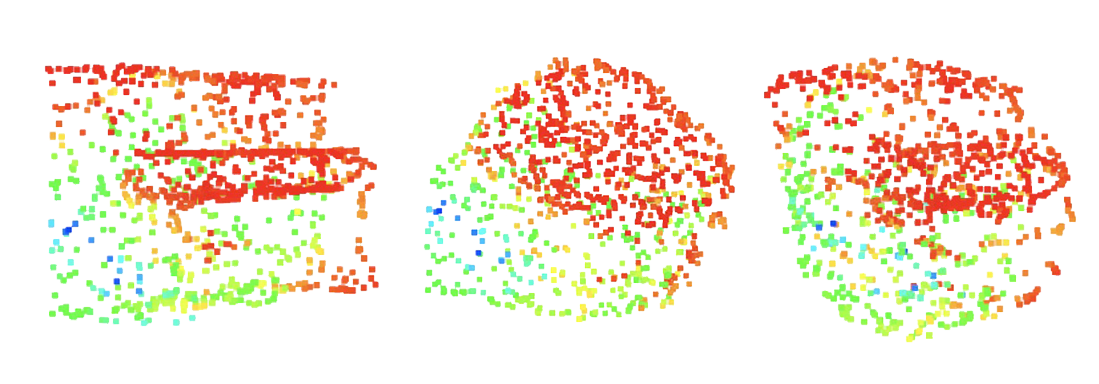
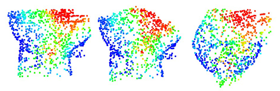
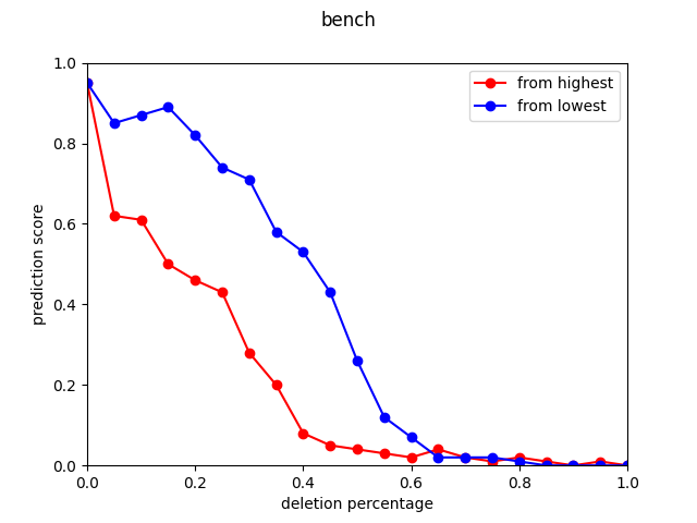
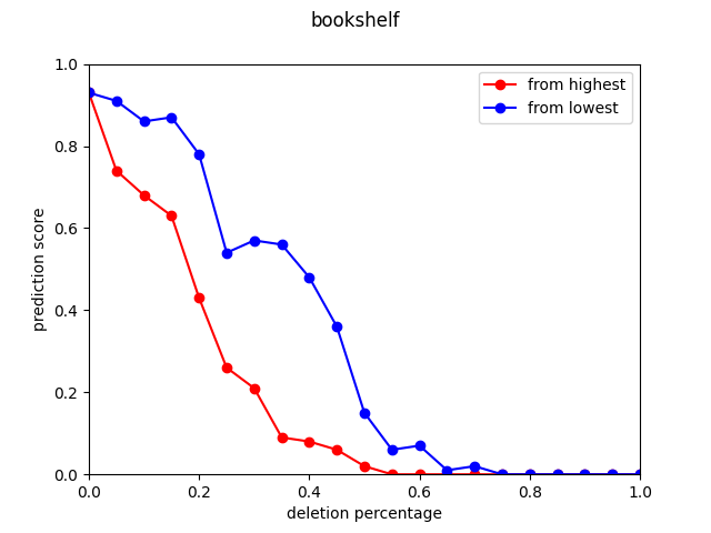
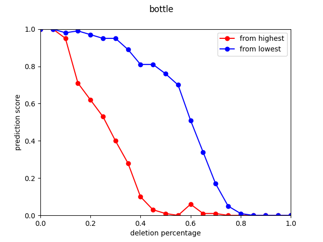
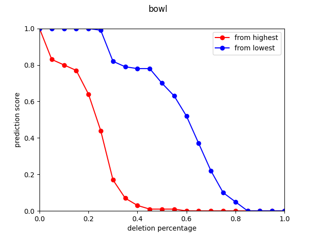
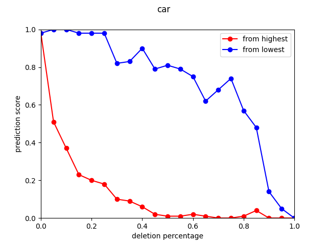
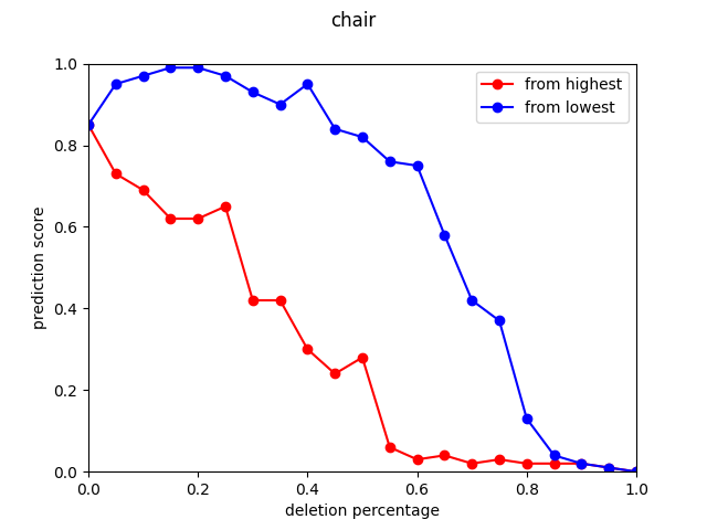
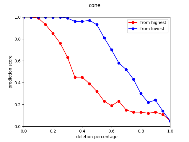
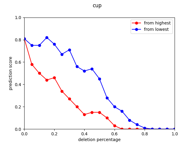
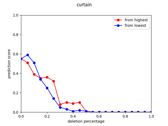
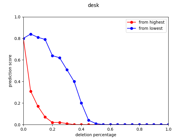
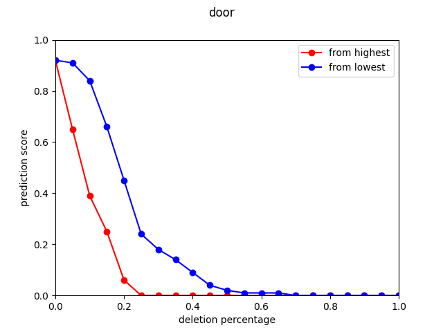
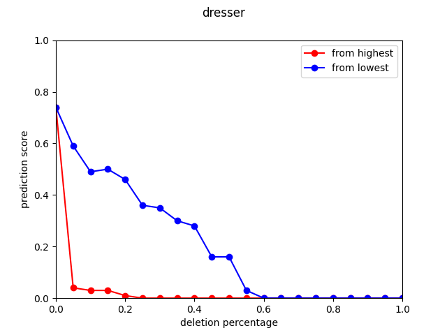
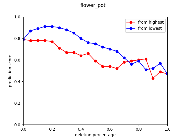
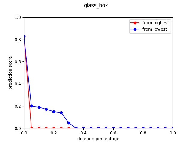
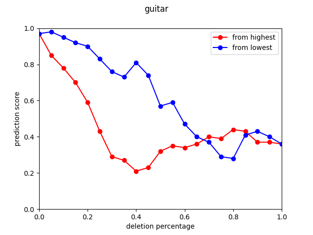
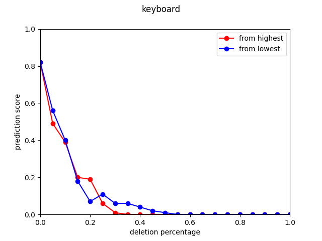
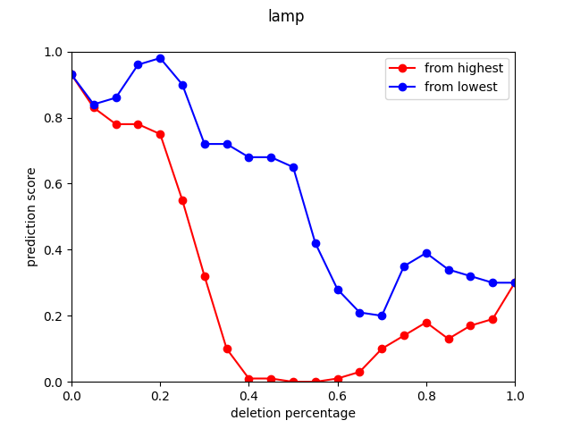
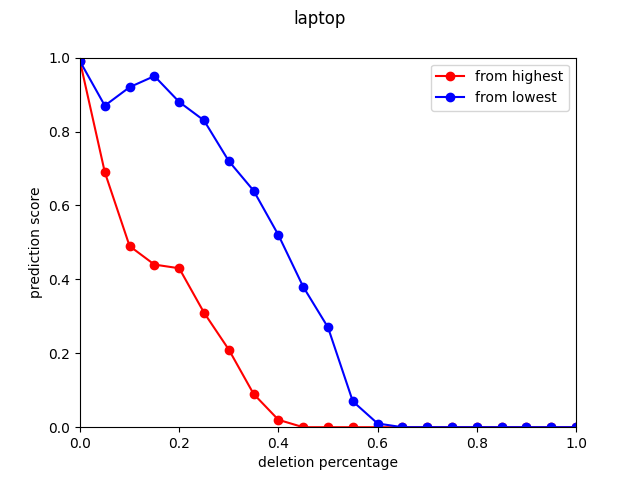
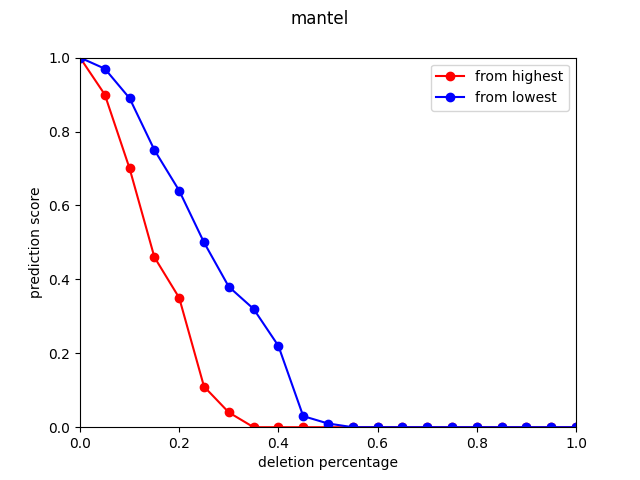
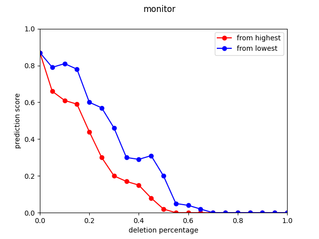
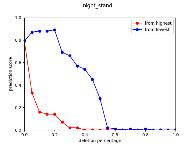
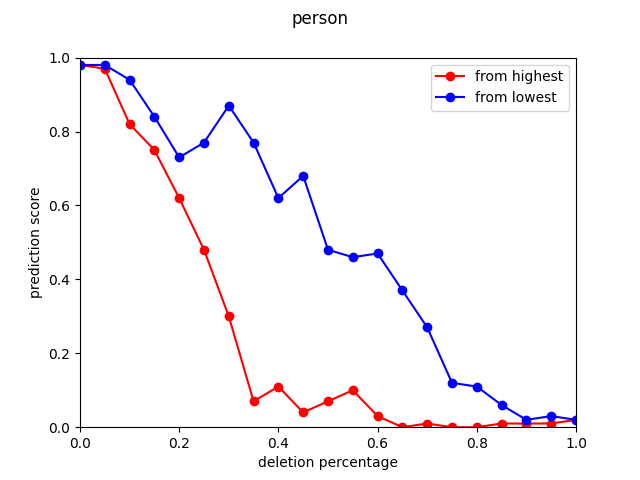
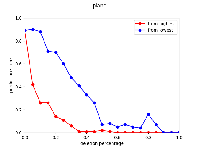
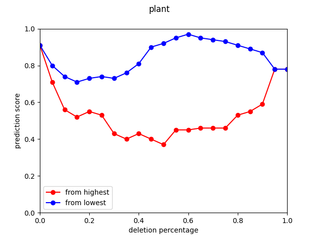
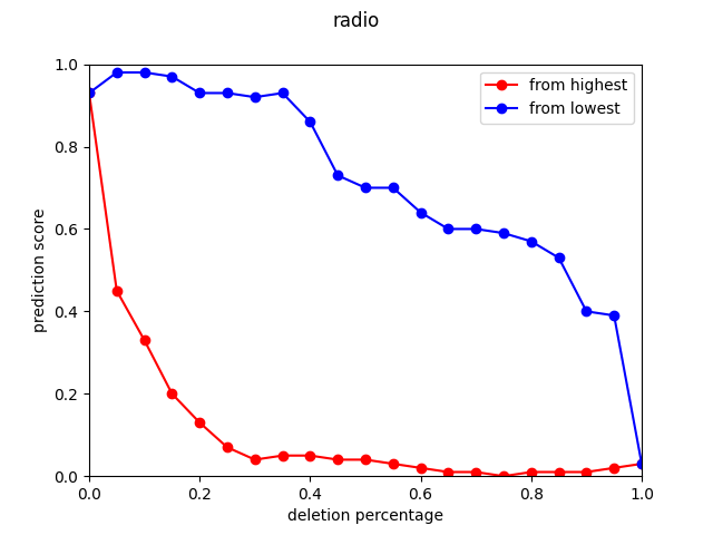
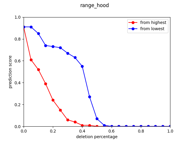
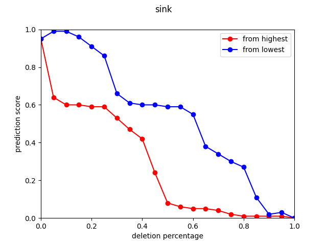
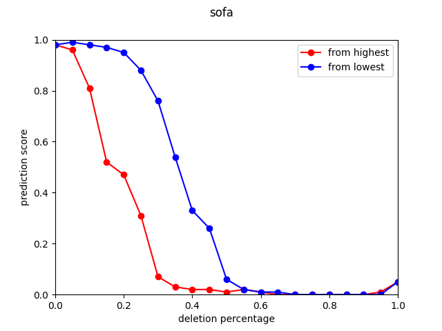
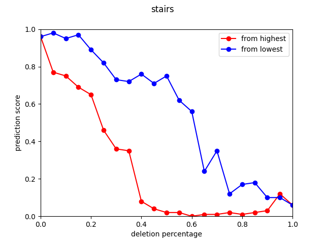
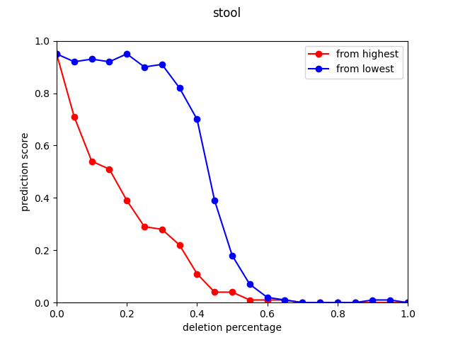
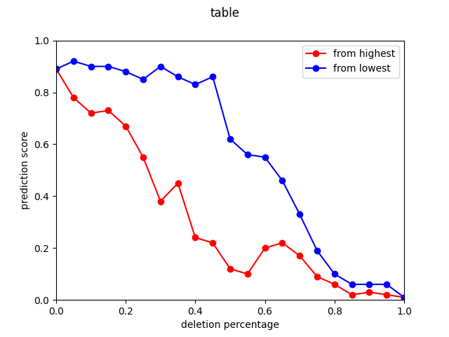
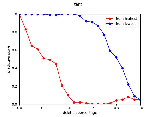
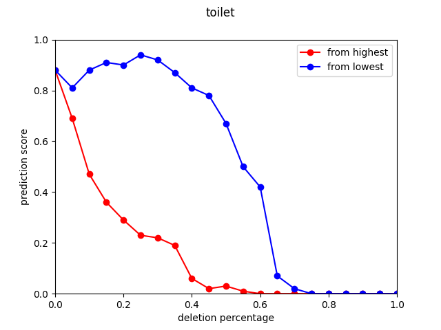
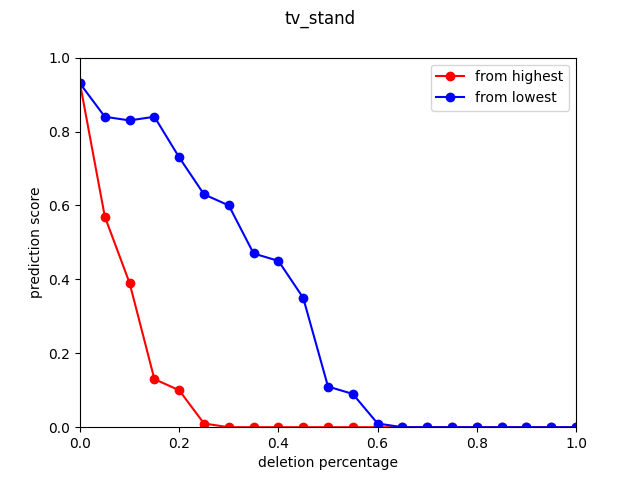
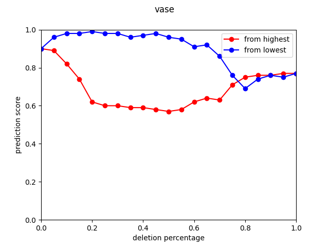
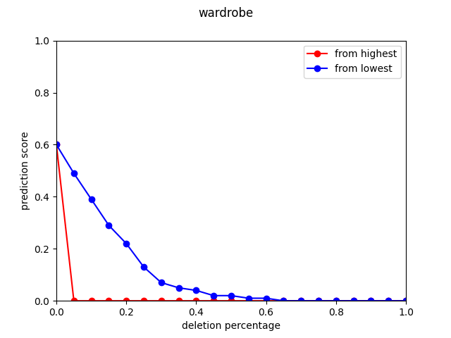
We experiment our PCI-GOS algorithm on PointConv [30], a state-of-the-art point cloud classifier, with the ModelNet 40 test set. We use the deletion and insertion metrics proposed by [19] to evaluate the heatmaps. Numbers displayed in the tables are the average scores along the deletion / insertion curves. Instead of point deletion / insertion, we use curvature deletion / insertion to evaluation our method. To delete top 5% curvature means smoothing only the top 5% points, and vice versa for insertion. The color scheme used for saliency map in picture illustrations: blue (0.0) green red (1.0).
Table 2 lists results of our algorithm compared to several baselines and [34]. Mask-only learns the mask using gradients instead of integrated gradients. Each mask goes through 300 iterations under this method, as opposed to 30 under PCI-GOS. Ig-only directly takes a one-step integrated gradient instead of an optimization process.
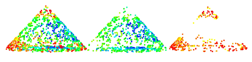
Our algorithm is optimized for curvature deletion/insertion, where curvature deletion means smoothing certain curved areas, and curvature insertion means smoothing all but those curved areas. It is shown that our approach outperforms both of these baselines. We also compare against Zheng et al. [34]. Here, note that the method in [34] is optimized for point deletion/insertion.To ensure fairness, we evaluate both methods on with both point and curvature del/ins. PC-IGOS and [34] give similar performance when respectively using their own evaluation method, and perform worse when using each other’s evaluation. As shown in Fig. 12, from our perspective, the most important feature for a tent is a flat ground, while from [34]’s perspective, the most important features are the points along the skeleton. It is difficult to argue from visual results which one is better, but we believe this has provided different perspectives of the point cloud classifier.
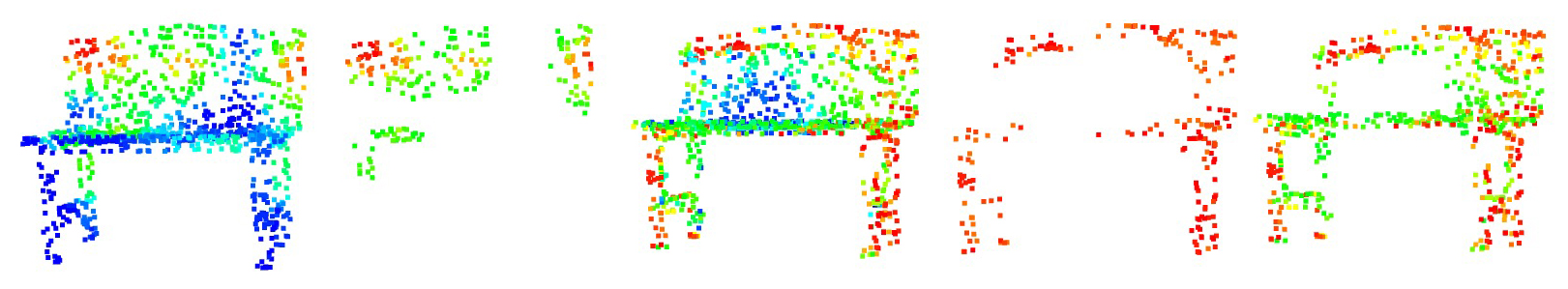
Interestingly, PCI-GOS improves over Zheng et al. [34] on both insertion metrics. We hypothesize that this might be because our algorithm tends to highlight an entire surface rather than concentrate on the edge of a shape (see Fig. 20). E.g., in the case of bookshelf, ModelNet40 contains many classes that have similar skeleton, such as dresser, wardrobe, etc. Thus, a sole rectangular frame might not be able to help the classifier to make decision.
Table 3 shows the ablation study for the -loss and the -loss (Eq. 8). Without the -loss, the deletion curve performs better and the insertion curve worse as expected, since the algorithm now concentrates on looking for points that drop the score quickly but not necessarily give rise to the score quickly. In practice, we also found a smaller mask size helps saliency learning. Usually, we train a mask size of 256 and upsample it to 1024 when applying in Equation 10. Ablation study shows that directly optimizing a mask of 1024 points leads to worse results, perhaps because the additional points make the optimization problem harder to solve.
For class-wise deletion and insertion curves, please refer to our supplementary material.
5 Conclusions and Future Work
In this paper, we propose a novel smoothing algorithm for morphing a point cloud into a shape with constant curvature, and PCI-GOS, a 3-D classifier visualization technique. We regard the most important contribution of this paper to be a new direction for point cloud network visualization – an optimization-based approach. It is a bit difficult to compare our method and [34] since the optimization goals are different. We generate quite different visualization results from prior work [34], but our insertion metrics are consistently higher than theirs, no matter evaluated using their methodology or ours. Additionally, our algorithm is more flexible with respect to learning goal. For example, by tuning up the coefficient of the -loss, we can obtain a mask that tends to highlight points capable of giving rise to prediction score quickly. We hope the visualization results in this paper improve the understanding on those new point cloud networks and we look forward to exploring better definitions of “non-informative” point clouds as well as smoothing with features beyond curvature in future work.
Acknowledgments
This work was partially supported by the National Science Foundation (NSF) under Project #1751402, USDA National Institute of Food and Agriculture (USDA-NIFA) under Award 2019-67019-29462, as well as by the Defense Advanced Research Projects Agency (DARPA) under Contract No. N66001-17-12-4030.
Appendix A Curvature approximation proof
Theorem 2.
Let be a point in point cloud. Let be the plane fitted to the neighbors of . Let be the projection of on . Assuming ’s neighbors distribute evenly and densely on a ring surrounding , then the curvature normal at can be approximated by the expression , where is the distance from to any of its neighbor.
Proof.
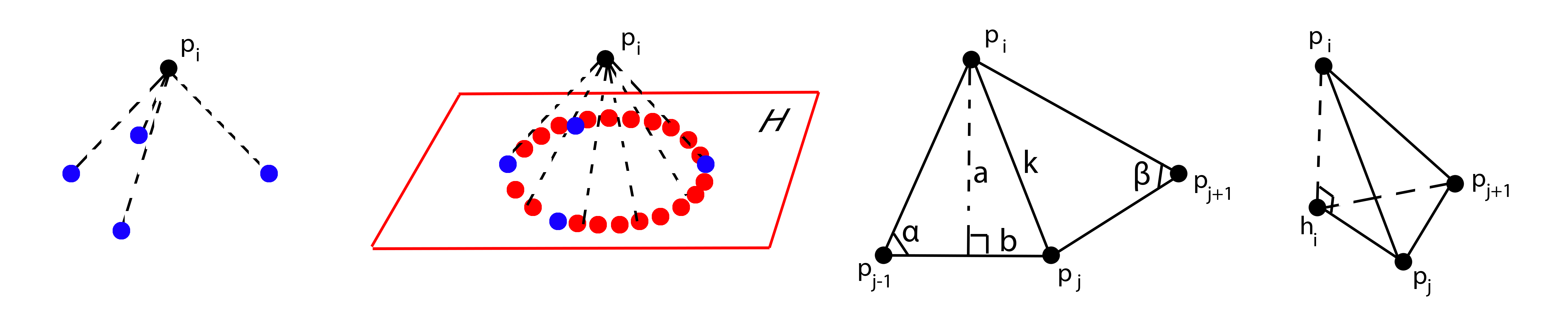
Our proof will refer to Fig. 28.
[7] has already showed that on a 3-D mesh, given a point and its neighbors, the local “carvature normal” can be calculated using
| (11) |
where is the sum of the areas of the triangles having as common vertex and are the two angles opposite to the edge (i.e. ). This arrangement is demonstrated Fig. 28.
Since point cloud data are usually sparse and noisy, we want to utilize some mechanism to mitigate this sparsity and irregularity. Here, we first fit a local plane to ’s neighborhood, and then we define the notion of “virtual neighbors” as a means to fill in the gaps left by the “actual neighbors”. We assume the “virtual neighbors” distribute evenly and densely on a ring surrounding on the fitted plane , each having the same distance to ( is calculated using the average distance of the actual neighbors). Let be the distance from to each edge . Let be half of the length of . Thus we can calculate in Eq. 11 as . Since we assumed the points are distributed evenly, we have . Thus we have the curvature normal to be .
Note that the vector is equal to , and it can be easily shown that . Thus we can continue derive the curvature normal to be . Since we assume the points are distributed densely, thus we have as , . Hence, the curvature normal at can be approximated by the expression
| (12) |
where is just the vector pointing from to the local plane as in Eq. 4. This equation makes sense in that when the distance from to is fixed, the further away the neighbors are, the “flatter” the surface at is. ∎
In our actual experimentation however, we found that due to the extremely irregular distribution of the point cloud data, the neighborhood distance is misleading sometimes rather than helpful. Thus, in our final algorithm, we abandon the distance information and directly use the vector pointing from to plane as our approximation for the local curvature.
Appendix B Implementation Details for Point cloud smoothing
An important implementation detail for the point cloud smoothing algorithm is that the size of the neighborhood we use increases as the smoothing goes further. In practice, after every 4 rounds of erosion and dilation, we expand the neighborhood size by points. The reason for this is twofold. On one hand, there might exist isolated neighborhoods in a point cloud (i.e. a set of points that is closed under the operation) as shown in Fig. 29. If the curvature information cannot be propagated to the entire point cloud, the algorithm will fail. On the other hand, a larger neighborhood speeds up the smoothing process. As mentioned in [12], the time step restriction results in the need of hundreds of updates to cause a noticeable smoothing using the original implementation in [28]. Note that however, we also cannot make the neighborhood size too large, especially at the beginning, due to the “false neighbor” issue innate to the point cloud data structure (explained in Fig. 30).
Appendix C Smoothing Algorithm Evaluation Metrics
In the experiment section of our paper, we use the following three metrics to compare our smoothing method against the baselines (Fig. 32, 33 and 34 show some example comparisons in pictures):
CSD. Curvature standard deviation. We regard large curvature on a shape as “features”, and we want to eliminate those “features” through the smoothing algorithms. As we remove the most distinct curvatures on the surface like edges and corners, the standard deviation of the curvatures will decrease, due to the elimination of the large outliers. In our experiment, we measure the distance from each point to its locally fitted plane () as an approximation of the local mean curvature.
MR. Min-max ratio. Assuming that the underlying manifold is closed, our smoothing should eventually morph the point cloud into a sphere. Hence, we propose to evaluate the ratio between the length on the short side and the long side of the point cloud. This is computed by first applying principal component analysis (PCA) to the point cloud and finding the top two principal components, say and . Then we compute the ratio between ranges of the values on these two principal directions. The closer this ratio is to 1, the better.
DDS. Density distribution similarity. We want the morphing process to be smooth in that the density distribution of each point cloud to remain the same throughout the morphing process. We conduct the kernel density estimation at each point (using a Gaussian kernel with ) to obtain the density distribution of the entire point cloud, and then compare the similarity between the distributions of two consecutive blurred levels using the Kolmogorov-Smirnov test (p-values are recorded as results).
Appendix D Curve figures
References
- [1] Marc Alexa, Johannes Behr, Daniel Cohen-Or, Shachar Fleishman, David Levin, and Claudio T Silva. Point set surfaces. In Proceedings of the Conference on Visualization’01, pages 21–28. IEEE Computer Society, 2001.
- [2] James Andrews and Carlo H Séquin. Type-constrained direct fitting of quadric surfaces. Computer-Aided Design and Applications, 11(1):107–119, 2014.
- [3] Matan Atzmon, Haggai Maron, and Yaron Lipman. Point convolutional neural networks by extension operators. arXiv preprint arXiv:1803.10091, 2018.
- [4] Sebastian Bach, Alexander Binder, Grégoire Montavon, Frederick Klauschen, Klaus-Robert Müller, and Wojciech Samek. On pixel-wise explanations for non-linear classifier decisions by layer-wise relevance propagation. PloS one, 10(7):e0130140, 2015.
- [5] Stéphane Calderon and Tamy Boubekeur. Point morphology. ACM Trans. Graph., 33(4):45:1–45:13, July 2014.
- [6] Piotr Dabkowski and Yarin Gal. Real time image saliency for black box classifiers. In Advances in Neural Information Processing Systems, pages 6967–6976, 2017.
- [7] Mathieu Desbrun, Mark Meyer, Peter Schröder, and Alan H Barr. Implicit fairing of irregular meshes using diffusion and curvature flow. In Proceedings of the 26th annual conference on Computer graphics and interactive techniques, pages 317–324. Citeseer, 1999.
- [8] Matthias Fey, Jan Eric Lenssen, Frank Weichert, and Heinrich Müller. Splinecnn: Fast geometric deep learning with continuous b-spline kernels. In Proceedings of the IEEE Conference on Computer Vision and Pattern Recognition, pages 869–877, 2018.
- [9] Ruth C. Fong and Andrea Vedaldi. Interpretable explanations of black boxes by meaningful perturbation. In The IEEE International Conference on Computer Vision (ICCV), Oct 2017.
- [10] Koji Fujiwara. Eigenvalues of laplacians on a closed riemannian manifold and its nets. Proceedings of the American Mathematical Society, 123(8):2585–2594, 1995.
- [11] Bennett Groshong, Griff Bilbro, and Wesley Snyder. Fitting a quadratic surface to three dimensional data. 1989.
- [12] Leif Kobbelt, Swen Campagna, Jens Vorsatz, and Hans-Peter Seidel. Interactive multi-resolution modeling on arbitrary meshes. In Siggraph, volume 98, pages 105–114, 1998.
- [13] David Levin. The approximation power of moving least-squares. Mathematics of computation, 67(224):1517–1531, 1998.
- [14] Yangyan Li, Rui Bu, Mingchao Sun, Wei Wu, Xinhan Di, and Baoquan Chen. Pointcnn: Convolution on x-transformed points. In Advances in Neural Information Processing Systems, pages 820–830, 2018.
- [15] Jyh-Ming Lien. Point-based minkowski sum boundary. In 15th Pacific Conference on Computer Graphics and Applications (PG’07), pages 261–270. IEEE, 2007.
- [16] Daniel Liu, Ronald Yu, and Hao Su. Extending adversarial attacks and defenses to deep 3d point cloud classifiers. arXiv preprint arXiv:1901.03006, 2019.
- [17] Zoltan Csaba Marton, Radu Bogdan Rusu, and Michael Beetz. On Fast Surface Reconstruction Methods for Large and Noisy Datasets. In Proceedings of the IEEE International Conference on Robotics and Automation (ICRA), Kobe, Japan, May 12-17 2009.
- [18] Boris Mederos, Luiz Velho, and Luiz Henrique de Figueiredo. Robust smoothing of noisy point clouds. In Proc. SIAM Conference on Geometric Design and Computing, volume 2004, page 2, 2003.
- [19] Vitali Petsiuk, Abir Das, and Kate Saenko. Rise: Randomized input sampling for explanation of black-box models. arXiv preprint arXiv:1806.07421, 2018.
- [20] Charles R. Qi, Li Yi, Hao Su, and Leonidas J. Guibas. Pointnet++: Deep hierarchical feature learning on point sets in a metric space. In Advances in Neural Information Processing Systems 30, pages 5099–5108. Curran Associates, Inc., 2017.
- [21] Zhongang Qi, Saeed Khorram, and Fuxin Li. Visualizing deep networks by optimizing with integrated gradients. In AAAI Conference on Artificial Intelligence, 2020.
- [22] Avanti Shrikumar, Peyton Greenside, Anna Shcherbina, and Anshul Kundaje. Not just a black box: Learning important features through propagating activation differences. arXiv preprint arXiv:1605.01713, 2016.
- [23] Karen Simonyan, Andrea Vedaldi, and Andrew Zisserman. Deep inside convolutional networks: Visualising image classification models and saliency maps. arXiv preprint arXiv:1312.6034, 2013.
- [24] Jost Tobias Springenberg, Alexey Dosovitskiy, Thomas Brox, and Martin Riedmiller. Striving for simplicity: The all convolutional net. arXiv preprint arXiv:1412.6806, 2014.
- [25] Hang Su, Varun Jampani, Deqing Sun, Subhransu Maji, Evangelos Kalogerakis, Ming-Hsuan Yang, and Jan Kautz. Splatnet: Sparse lattice networks for point cloud processing. In Proceedings of the IEEE Conference on Computer Vision and Pattern Recognition, pages 2530–2539, 2018.
- [26] Mukund Sundararajan, Ankur Taly, and Qiqi Yan. Axiomatic attribution for deep networks. In Proceedings of the 34th International Conference on Machine Learning - Volume 70, ICML’17, pages 3319–3328. JMLR.org, 2017.
- [27] Maxim Tatarchenko, Jaesik Park, Vladlen Koltun, and Qian-Yi Zhou. Tangent convolutions for dense prediction in 3d. In Proceedings of the IEEE Conference on Computer Vision and Pattern Recognition, pages 3887–3896, 2018.
- [28] Gabriel Taubin. A signal processing approach to fair surface design. In Proceedings of the 22Nd Annual Conference on Computer Graphics and Interactive Techniques, SIGGRAPH ’95, pages 351–358, New York, NY, USA, 1995. ACM.
- [29] Yue Wang, Yongbin Sun, Ziwei Liu, Sanjay E Sarma, Michael M Bronstein, and Justin M Solomon. Dynamic graph cnn for learning on point clouds. arXiv preprint arXiv:1801.07829, 2018.
- [30] Wenxuan Wu, Zhongang Qi, and Li Fuxin. Pointconv: Deep convolutional networks on 3d point clouds. In The IEEE Conference on Computer Vision and Pattern Recognition (CVPR), June 2019.
- [31] Chong Xiang, Charles R Qi, and Bo Li. Generating 3d adversarial point clouds. In Proceedings of the IEEE Conference on Computer Vision and Pattern Recognition, pages 9136–9144, 2019.
- [32] Yifan Xu, Tianqi Fan, Mingye Xu, Long Zeng, and Yu Qiao. Spidercnn: Deep learning on point sets with parameterized convolutional filters. In Proceedings of the European Conference on Computer Vision (ECCV), pages 87–102, 2018.
- [33] Matthew D Zeiler and Rob Fergus. Visualizing and understanding convolutional networks. In European conference on computer vision, pages 818–833. Springer, 2014.
- [34] Tianhang Zheng, Changyou Chen, Junsong Yuan, Bo Li, and Kui Ren. Pointcloud saliency maps. In The IEEE International Conference on Computer Vision (ICCV), October 2019.
- [35] Bolei Zhou, Aditya Khosla, Agata Lapedriza, Aude Oliva, and Antonio Torralba. Object detectors emerge in deep scene cnns. arXiv preprint arXiv:1412.6856, 2014.
- [36] Kehe Zhu. Operator theory in function spaces. Number 138. American Mathematical Soc., 2007.