SAL: Sign Agnostic Learning of Shapes from Raw Data

Abstract

Recently, neural networks have been used as implicit representations for surface reconstruction, modelling, learning, and generation. So far, training neural networks to be implicit representations of surfaces required training data sampled from a ground-truth signed implicit functions such as signed distance or occupancy functions, which are notoriously hard to compute.

In this paper we introduce Sign Agnostic Learning (SAL), a deep learning approach for learning implicit shape representations directly from raw, unsigned geometric data, such as point clouds and triangle soups.

We have tested SAL on the challenging problem of surface reconstruction from an un-oriented point cloud, as well as end-to-end human shape space learning directly from raw scans dataset, and achieved state of the art reconstructions compared to current approaches. We believe SAL opens the door to many geometric deep learning applications with real-world data, alleviating the usual painstaking, often manual pre-process.

1 Introduction

Recently, deep neural networks have been used to reconstruct, learn and generate 3D surfaces. There are two main approaches: parametric [20, 5, 43, 16] and implicit [13, 32, 30, 3, 15, 18]. In the parametric approach neural nets are used as parameterization mappings, while the implicit approach represents surfaces as zero level-sets of neural networks:

$${\mathcal{S}}=\left\{{\bm{x}}\in\mathbb{R}^{3}\ |\ f({\bm{x}};{\bm{\theta}})=0\right\},$$ (1)

where $f:\mathbb{R}^{3}\times\mathbb{R}^{m}\rightarrow\mathbb{R}$ is a neural network, e.g., multilayer perceptron (MLP). The benefit in using neural networks as implicit representations to surfaces stems from their flexibility and approximation power (e.g., Theorem 1 in [3]) as well as their efficient optimization and generalization properties.

So far, neural implicit surface representations were mostly learned using a regression-type loss, requiring data samples from a ground-truth implicit representation of the surface, such as a signed distance function [32] or an occupancy function [13, 30]. Unfortunately, for the common raw form of acquired 3D data ${\mathcal{X}}\subset\mathbb{R}^{3}$, i.e., a point cloud or a triangle soup, no such data is readily available and computing an implicit ground-truth representation for the underlying surface is a notoriously difficult task [6].

In this paper we advocate Sign Agnostic Learning (SAL), defined by a family of loss functions that can be used directly with raw (unsigned) geometric data ${\mathcal{X}}$ and produce signed implicit representations of surfaces. An important application for SAL is in generative models such as variational auto-encoders [26], learning shape spaces directly from the raw 3D data. Figure 1 depicts an example where collectively learning a dataset of raw human scans using SAL overcomes many imperfections and artifacts in the data (left in every gray pair) and provides high quality surface reconstructions (right in every gray pair) and shape space (interpolations of latent representations are in gold).

We have experimented with SAL for surface reconstruction from point clouds as well as learning a human shape space from the raw scans of the D-Faust dataset [8]. Comparing our results to current approaches and baselines we found SAL to be the method of choice for learning shapes from raw data, and believe SAL could facilitate many computer vision and computer graphics shape learning applications, allowing the user to avoid the tedious and unsolved problem of surface reconstruction in preprocess. Our code is available at https://github.com/matanatz/SAL.

2 Previous work

2.1 Surface learning with neural networks

Neural parameteric surfaces.

One approach to represent surfaces using neural networks is parametric, namely, as parameterization charts $f:\mathbb{R}^{2}\rightarrow\mathbb{R}^{3}$. Groueix et al. [20] suggest to represent a surface using a collection of such parameterization charts (i.e., atlas); Williams et al. [43] optimize an atlas with proper transition functions between charts and concentrate on reconstructions of individual surfaces. Sinha et al. [35, 36] use geometry images as global parameterizations, while [29] use conformal global parameterizations to reduce the number of degrees of freedom of the map. Parametric representation are explicit but require handling of coverage, overlap and distortion of charts.

Neural implicit surfaces.

Another approach to represent surfaces using neural networks, which is also the approach taken in this paper, is using an implicit representation, namely $f:\mathbb{R}^{3}\rightarrow\mathbb{R}$ and the surface is defined as its zero level-set, equation 1. Some works encode $f$ on a volumetric grid such as voxel grid [44] or an octree [39]. More flexibility and potentially more efficient use of the degrees of freedom of the model are achieved when the implicit function $f$ is represented as a neural network [13, 32, 30, 3, 18]. In these works the implicit is trained using a regression loss of the signed distance function [32], an occupancy function [13, 30] or via particle methods to directly control the neural level-sets [3]. Excluding the latter that requires sampling the zero level-set, all regression-based methods require ground-truth inside/outside information to train the implicit $f$. In this paper we present a sign agnostic training method, namely training method that can work directly with the raw (unsigned) data.

Shape representation learning.

Learning collections of shapes is done using Generative Adversarial Networks (GANs) [19], auto-encoders and variational auto-encoders [26], and auto-decoders [9]. Wu et al. [44] use GAN on a voxel grid encoding of the shape, while Ben-Hamu et al. [5] apply GAN on a collection of conformal charts. Dai et al. [14] use encoder-decoder architecture to learn a signed distance function to a complete shape from a partial input on a volumetric grid. Stutz et al. [37] use variational auto-encoder to learn an implicit surface representations of cars using a volumetric grid. Baqautdinov et al. [4] use variational auto-encoder with a constant mesh to learn parametrizations of faces shape space. Litany et al. [27] use variational auto-encoder to learn body shape embeddings of a template mesh. Park et al. [32] use auto-decoder to learn implicit neural representations of shapes, namely directly learns a latent vector for every shape in the dataset. In our work we also make use of a variational auto-encoder but differently from previous work, learning is done directly from raw 3D data.

2.2 Surface reconstruction.

Signed surface reconstruction.

Many surface reconstruction methods require normal or inside/outside information. Carr et al. [10] were among the first to suggest using a parametric model to reconstruct a surface by computing its implicit representation; they use radial basis functions (RBFs) and regress at inside and outside points computed using oriented normal information. Kazhdan et al. [23, 24] solve a Poisson equation on a volumetric discretization to extend points and normals information to an occupancy indicator function. Walder et al. [41] use radial basis functions and solve a variational hermite problem (i.e., fitting gradients of the implicit to the normal data) to avoid trivial solution. In general our method works with a non-linear parameteric model (MLP) and therefore does not require a-priori space discretization nor works with a fixed linear basis such as RBFs.

Unsigned surface reconstruction.

More related to this paper are surface reconstruction methods that work with unsigned data such as point clouds and triangle soups. Zhao et al. [47] use the level-set method to fit an implicit surface to an unoriented point cloud by minimizing a loss penalizing distance of the surface to the point cloud achieving a sort of minimal area surface interpolating the points. Walder et al. [40] formulates a variational problem fitting an implicit RBF to an unoriented point cloud data while minimizing a regularization term and maximizing the norm of the gradients; solving the variational problem is equivalent to an eigenvector problem. Mullen et al. [31] suggests to sign an unsigned distance function to a point cloud by a multi-stage algorithm first dividing the problem to near and far field sign estimation, and propagating far field estimation closer to the zero level-set; then optimize a convex energy fitting a smooth sign function to the estimated sign function. Takayama et al. [38] suggested to orient triangle soups by minimizing the Dirichlet energy of the generalized winding number noting that correct orientation yields piecewise constant winding number. Xu et al. [45] suggested to compute robust signed distance function to triangle soups by using an offset surface defined by the unsigned distance function. Zhiyang et al. [22] fit an RBF implicit by optimizing a non-convex variational problem minimizing smoothness term, interpolation term and unit gradient at data points term. All these methods use some linear function space; when the function space is global, e.g. when using RBFs, model fitting and evaluation are costly and limit the size of point clouds that can be handled efficiently, while local support basis functions usually suffer from inferior smoothness properties [42]. In contrast we use a non-linear function basis (MLP) and advocate a novel and simple sign agnostic loss to optimize it. Evaluating the non-linear neural network model is efficient and scalable and the training process can be performed on a large number of points, e.g., with stochastic optimization techniques.

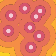
(a)	(b)
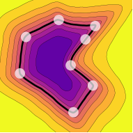
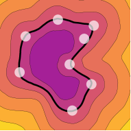
(c)	(d)

Figure 2: Experiment with sign agnostic learning in 2D: (a) and (b) show the unsigned $L^{0}$ and $L^{2}$ (resp.) distances to a 2D point cloud (in gray); (c) and (d) visualize the different level-sets of the neural networks optimized with the respective sign agnostic losses. Note how the zero level-sets (in bold) gracefully connect the points to complete the shape.

3 Sign agnostic learning

Given a raw input geometric data, ${\mathcal{X}}\subset\mathbb{R}^{3}$, e.g., a point cloud or a triangle soup, we are looking to optimize the weights ${\bm{\theta}}\in\mathbb{R}^{m}$ of a network $f({\bm{x}};{\bm{\theta}})$, where $f:\mathbb{R}^{3}\times\mathbb{R}^{m}\rightarrow\mathbb{R}$, so that its zero level-set, equation 1, is a surface approximating ${\mathcal{X}}$.

We introduce the Sign Agnostic Learning (SAL) defined by a loss of the form

$$\mathrm{loss}({\bm{\theta}})=\mathbb{E}_{{\bm{x}}\sim D_{\mathcal{X}}}\ \tau\Big{(}f({\bm{x}};{\bm{\theta}}),h_{\mathcal{X}}({\bm{x}})\Big{)},$$ (2)

where $D_{\mathcal{X}}$ is a probability distribution defined by the input data ${\mathcal{X}}$; $h_{\mathcal{X}}({\bm{x}})$ is some unsigned distance measure to ${\mathcal{X}}$; and $\tau:\mathbb{R}\times\mathbb{R}_{+}\rightarrow\mathbb{R}$ is a differentiable unsigned similarity function defined by the following properties:

1. Sign agnostic: $\tau(-a,b)=\tau(a,b)$, $\forall a\in\mathbb{R}$, $b\in\mathbb{R}_{+}$.

2. Monotonic: $\frac{\partial\tau}{\partial a}(a,b)=\rho(a-b)$, $\forall a,b\in\mathbb{R}_{+}$,

where $\rho:\mathbb{R}\rightarrow\mathbb{R}$ is a monotonically increasing function with $\rho(0)=0$. An example of an unsigned similarity is $\tau(a,b)=\left|\left|a\right|-b\right|$.

To understand the idea behind the definition of the SAL loss, consider first a standard regression loss using $\tau(a,b)=\left|a-b\right|$ in equation 2. This would encourage $f$ to resemble the unsigned distance $h_{\mathcal{X}}$ as much as possible. On the other hand, using the unsigned similarity $\tau$ in equation 2 introduces a new local minimum of $\mathrm{loss}$ where $f$ is a signed function such that $\left|f\right|$ approximates $h_{\mathcal{X}}$. To get this desirable local minimum we later design a network weights’ initialization ${\bm{\theta}}^{0}$ that favors the signed local minima.

As an illustrative example, the inset depicts the one dimensional case ($d=1$) where ${\mathcal{X}}=\left\{x_{0}\right\}$, $h_{\mathcal{X}}(x)=|x-x_{0}|$, and $\tau(a,b)=\left|\left|a\right|-b\right|$, which satisfies properties (i) and (ii), as discussed below; the loss therefore strives to minimize the area of the yellow set. When initializing the network parameters ${\bm{\theta}}={\bm{\theta}}^{0}$ properly, the minimizer ${\bm{\theta}}^{*}$ of $\mathrm{loss}$ defines an implicit $f(x;{\bm{\theta}}^{*})$ that realizes a signed version of $h_{\mathcal{X}}$; in this case $f(x;{\bm{\theta}}^{*})=x-x_{0}$. In the three dimensional case the zero level-set ${\mathcal{S}}$ of $f({\bm{x}};{\bm{\theta}}^{*})$ will represent a surface approximating ${\mathcal{X}}$.

To theoretically motivate the loss family in equation 2 we will prove that it possess a plane reproduction property. That is, if the data ${\mathcal{X}}$ is contained in a plane, there is a critical weight ${\bm{\theta}}^{*}$ reconstructing this plane as the zero level-set of $f({\bm{x}};{\bm{\theta}}^{*})$. Plane reproduction is important for surface approximation since surfaces, by definition, have an approximate tangent plane almost everywhere [17].

We will explore instantiations of SAL based on different choices of unsigned distance functions $h_{\mathcal{X}}$, as follows.

Unsigned distance functions.

We consider two $p$-distance functions: For $p=2$ we have the standard $L^{2}$ (Euclidean) distance

$$h_{2}({\bm{z}})=\min_{{\bm{x}}\in{\mathcal{X}}}\left\|{\bm{z}}-{\bm{x}}\right\|_{2},$$ (3)

and for $p=0$ the $L^{0}$ distance

$$h_{0}({\bm{z}})=\begin{cases}0&{\bm{z}}\in{\mathcal{X}}\\ 1&{\bm{z}}\notin{\mathcal{X}}\end{cases}.$$ (4)

Unsigned similarity function.

Although many choices exist for the unsigned similarity function, in this paper we take

$$\tau_{\ell}(a,b)=\left|\left|a\right|-b\right|^{\ell},$$ (5)

where $\ell\geq 1$. The function $\tau_{\ell}$ is indeed an unsigned similarity: it satisfies (i) due to the symmetry of $\left|\cdot\right|$; and since $\frac{\partial\tau}{\partial a}=\ell\left||a|-b\right|^{\ell-1}\mathrm{sign}(a-b\,\mathrm{sign}(a))$ it satisfies (ii) as-well.

Distribution $D_{\mathcal{X}}$.

The choice of $D_{\mathcal{X}}$ is depending on the particular choice of $h_{\mathcal{X}}$. For $L^{2}$ distance, it is enough to make the simple choice of splatting an isotropic Gaussian, ${\mathcal{N}}({\bm{x}},\sigma^{2}I)$, at every point (uniformly randomized) ${\bm{x}}\in{\mathcal{X}}$; we denote this probability ${\mathcal{N}}_{\sigma}({\mathcal{X}})$; note that $\sigma$ can be taken to be a function of ${\bm{x}}\in{\mathcal{X}}$ to reflect local density in ${\mathcal{X}}$. In this case, the loss takes the form

$$\mathrm{loss}({\bm{\theta}})=\mathbb{E}_{{\bm{z}}\sim{\mathcal{N}}_{\sigma}({\mathcal{X}})}\big{|}|f({\bm{z}};{\bm{\theta}})|-h_{2}({\bm{z}})\big{|}^{\ell}.$$ (6)

For the $L^{0}$ distance however, $h_{\mathcal{X}}({\bm{x}})\neq 1$ only for ${\bm{x}}\in{\mathcal{X}}$ and therefore a non-continuous density should be used; we opt for ${\mathcal{N}}({\bm{x}},\sigma^{2}I)+\delta_{\bm{x}}$, where $\delta_{\bm{x}}$ is the delta distribution measure concentrated at ${\bm{x}}$. The loss takes the form

$$\mathrm{loss}({\bm{\theta}})=\mathbb{E}_{{\bm{z}}\sim{\mathcal{N}}_{\sigma}({\mathcal{X}})}\big{|}|f({\bm{z}};{\bm{\theta}})|-1\big{|}^{\ell}+\mathbb{E}_{{\bm{x}}\sim{\mathcal{X}}}\big{|}f({\bm{x}};{\bm{\theta}})\big{|}^{\ell}.$$ (7)

Remarkably, the latter loss requires only randomizing points ${\bm{z}}$ near the data samples without any further computations involving ${\mathcal{X}}$. This allows processing of large and/or complex geometric data.

Neural architecture.

Although SAL can work with different parametric models, in this paper we consider a multilayer perceptron (MLP) defined by

$$f({\bm{x}};{\bm{\theta}})=\varphi\big{(}{\bm{w}}^{T}f_{\ell}\circ f_{\ell-1}\circ\cdots\circ f_{1}({\bm{x}})+b\big{)},$$ (8)

and

$$f_{i}({\bm{y}})=\nu({\bm{W}}_{i}{\bm{y}}+{\bm{b}}_{i}),{\bm{W}}\in\mathbb{R}^{d_{i}^{out}\times d_{i}^{in}},{\bm{b}}_{i}\in\mathbb{R}^{d_{i}^{out}},$$ (9)

where $\nu(a)=(a)_{+}$ is the ReLU activation, and ${\bm{\theta}}=({\bm{w}},b,{\bm{W}}_{\ell},{\bm{b}}_{\ell},\ldots,{\bm{W}}_{1},{\bm{b}}_{1})$; $\varphi$ is a strong non-linearity, as defined next:

Definition 1.

The function $\varphi:\mathbb{R}\rightarrow\mathbb{R}$ is called a strong non-linearity if it is differentiable (almost everywhere), anti-symmetric, $\varphi(-a)=-\varphi(a)$, and there exists $\beta\in\mathbb{R}_{+}$ so that $\beta^{-1}\geq\varphi^{\prime}(a)\geq\beta>0$, for all $a\in\mathbb{R}$ where it is defined.

In this paper we use $\varphi(a)=a$ or $\varphi(a)=\tanh(a)+\gamma a$, where $\gamma\geq 0$ is a parameter. Furthermore, similarly to previous work [32, 13] we have incorporated a skip connection layer $s$, concatenating the input ${\bm{x}}$ to the middle hidden layer, that is $s({\bm{y}})=({\bm{y}},{\bm{x}})$, where here ${\bm{y}}$ is a hidden variable in $f$.

2D example.

The two examples in Figure 2 show case the SAL for a 2D point cloud, ${\mathcal{X}}=\left\{{\bm{x}}_{i}\right\}_{i=1}^{8}\subset\mathbb{R}^{2}$, (shown in gray) as input. These examples were computed by optimizing equation 6 (right column) and equation 7 (left column) with $\ell=1$ using the $L^{2}$ and $L^{0}$ distances (resp.). The architecture used is an 8-layer MLP; all hidden layers are 100 neurons wide, with a skip connection to the middle layer.

Notice that both $h_{\mathcal{X}}({\bm{x}})$ and its signed version are local minima of the loss in equation 2. These local minima are stable in the sense that there is an energy barrier when moving from one to the other. For example, to get to a solution as in Figure 2(b) from the solution in Figure 2(d) one needs to flip the sign in the interior or exterior of the region defined by the black line. Changing the sign continuously will result in a considerable increase to the SAL loss value.

We elaborate on our initialization method, ${\bm{\theta}}={\bm{\theta}}^{0}$, that in practice favors the signed version of $h_{\mathcal{X}}$ in the next section.

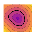
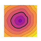
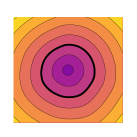
(a)	(b)	(c)

Figure 3: Geometric initialization of neural networks: An MLP with our weight initialization (see Theorem 1) is approximating the signed distance function to an $r$-radius sphere, $f({\bm{x}};{\bm{\theta}}^{0})\approx\varphi(\left\|{\bm{x}}\right\|-r)$, where the approximation improves with the width of the hidden layers: (a) depicts an MLP with $100$-neuron hidden layers; (b) with $200$; and (c) with $2000$.

4 Geometric network initialization

A key aspect of our method is a proper, geometrically motivated initialization of the network’s parameters. For MLPs, equations 8-9, we develop an initialization of its parameters, ${\bm{\theta}}={\bm{\theta}}^{0}$, so that $f({\bm{x}};{\bm{\theta}}^{0})\approx\varphi(\left\|{\bm{x}}\right\|-r)$, where $\left\|{\bm{x}}\right\|-r$ is the signed distance function to an $r$-radius sphere. The following theorem specify how to pick ${\bm{\theta}}^{0}$ to achieve this:

Theorem 1.

Let $f$ be an MLP (see equations 8-9). Set, for $1\leq i\leq\ell$, ${\bm{b}}_{i}=0$ and ${\bm{W}}_{i}$ i.i.d. from a normal distribution ${\mathcal{N}}(0,\frac{\sqrt{2}}{\sqrt{d_{i}^{out}}})$; further set ${\bm{w}}={\frac{\sqrt{\pi}}{\sqrt{d_{\ell}^{out}}}}\mathbf{1}$, $c=-r$. Then, $f({\bm{x}})\approx\varphi(\left\|x\right\|-r)$.

Figure 3 depicts level-sets (zero level-sets in bold) using the initialization of Theorem 1 with the same 8-layer MLP (using $\varphi(a)=a$) and increasing width of 100, 200, and 2000 neurons in the hidden layers. Note how the approximation $f({\bm{x}};{\bm{\theta}}^{0})\approx\left\|{\bm{x}}\right\|-r$ improves as the layers’ width increase, while the sphere-like (in this case circle-like) zero level-set remains topologically correct at all approximation levels.

The proof to Theorem 1 is provided in the supplementary material; it is a corollary of the following theorem, showing how to chose the initial weights for a single hidden layer network:

Theorem 2.

Let $f:\mathbb{R}^{d}\rightarrow\mathbb{R}$ be an MLP with ReLU activation, $\nu$, and a single hidden layer. That is, $f({\bm{x}})={\bm{w}}^{T}\nu({\bm{W}}{\bm{x}}+{\bm{b}})+c$, where ${\bm{W}}\in\mathbb{R}^{d^{out}\times d}$, ${\bm{b}}\in\mathbb{R}^{d^{out}}$, ${\bm{w}}\in\mathbb{R}^{d^{out}}$, $c\in\mathbb{R}$ are the learnable parameters. If ${\bm{b}}=0$, ${\bm{w}}=\frac{\sqrt{2\pi}}{\sigma d^{out}}\mathbf{1}$, $c=-r$, $r>0$, and all entries of ${\bm{W}}$ are i.i.d. normal ${\mathcal{N}}(0,\sigma^{2})$ then $f({\bm{x}})\approx\left\|{\bm{x}}\right\|-r$. That is, $f$ is approximately the signed distance function to a $d-1$ sphere of radius $r$ in $\mathbb{R}^{d}$, centered at the origin.

5 Properties

5.1 Plane reproduction

Plane reproduction is a key property to surface approximation methods since, in essence, surfaces are locally planar, i.e., have an approximating tangent plane almost everywhere [17]. In this section we provide a theoretical justification to SAL by proving a plane reproduction property. We first show this property for a linear model (i.e., a single layer MLP) and then show how this implies local plane reproduction for general MLPs.

The setup is as follows: Assume the input data ${\mathcal{X}}\subset\mathbb{R}^{d}$ lies on a hyperplane ${\mathcal{X}}\subset{\mathcal{P}}$, where ${\mathcal{P}}=\left\{{\bm{x}}\in\mathbb{R}^{d}\ |\ {\bm{n}}^{T}{\bm{x}}+c=0\right\}$, ${\bm{n}}\in\mathbb{R}^{d}$, $\left\|{\bm{n}}\right\|=1$, is the normal to the plane, and consider a linear model $f({\bm{x}};{\bm{w}},b)=\varphi({\bm{w}}^{T}{\bm{x}}+b)$. Furthermore, we make the assumption that the distribution $D_{\mathcal{X}}$ and the distance $h_{\mathcal{X}}$ are invariant to rigid transformations, which is common and holds in all cases considered in this paper. We prove existence of critical weights $({\bm{w}}^{*},b^{*})$ of the loss in equation 2, and for which the zero level-set of $f$, $f({\bm{x}};{\bm{w}}^{*},b^{*})=0$, reproduces ${\mathcal{P}}$:

Theorem 3.

Consider a linear model $f({\bm{x}};{\bm{\theta}})=\varphi({\bm{w}}^{T}{\bm{x}}+b)$, ${\bm{\theta}}=({\bm{w}},b)$, with a strong non-linearity $\varphi:\mathbb{R}\rightarrow\mathbb{R}$. Assume the data ${\mathcal{X}}$ lies on a plane ${\mathcal{P}}=\left\{{\bm{x}}|{\bm{n}}^{T}{\bm{x}}+c=0\right\}$, i.e., ${\mathcal{X}}\subset{\mathcal{P}}$. Then, there exists $\alpha\in\mathbb{R}_{+}$ so that $({\bm{w}}^{*},b^{*})=(\alpha{\bm{n}},\alpha c)$ is a critical point of the loss in equation 2.

This theorem can be applied locally when optimizing a general MLP (equation 8) with SAL to prove local plane reproduction. See supplementary for more details.

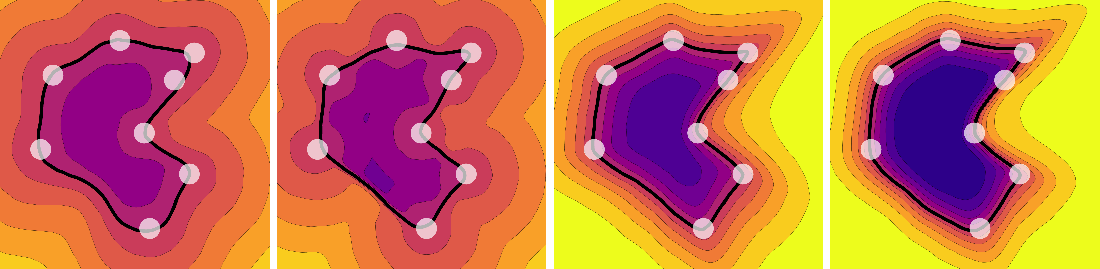
Figure 4: Advanced epochs of the neural level-sets from Figure 2. The limit in the $L^{0}$ case (two right images) is an inside/outside indicator function, while for the $L^{2}$ case (two left images) it is a signed version of the unsigned $L^{2}$ distance.

5.2 Convergence to the limit signed function

The SAL loss pushes the neural implicit function $f$ towards a signed version of the unsigned distance function $h_{\mathcal{X}}$. In the $L^{0}$ case it is the inside/outside indicator function of the surface, while for $L^{2}$ it is a signed version of the Euclidean distance to the data ${\mathcal{X}}$. Figure 4 shows advanced epochs of the 2D experiment in Figure 2; note that the $f$ in these advanced epochs is indeed closer to the signed version of the respective $h_{\mathcal{X}}$. Since the indicator function and the signed Euclidean distance are discontinuous across the surface, they potentially impose quantization errors when using standard contouring algorithms, such as Marching Cubes [28], to extract their zero level-set. In practice, this phenomenon is avoided with a standard choice of stopping criteria (learning rate and number of iterations). Another potential solution is to add a regularization term to the SAL loss; we mark this as future work.

6 Experiments

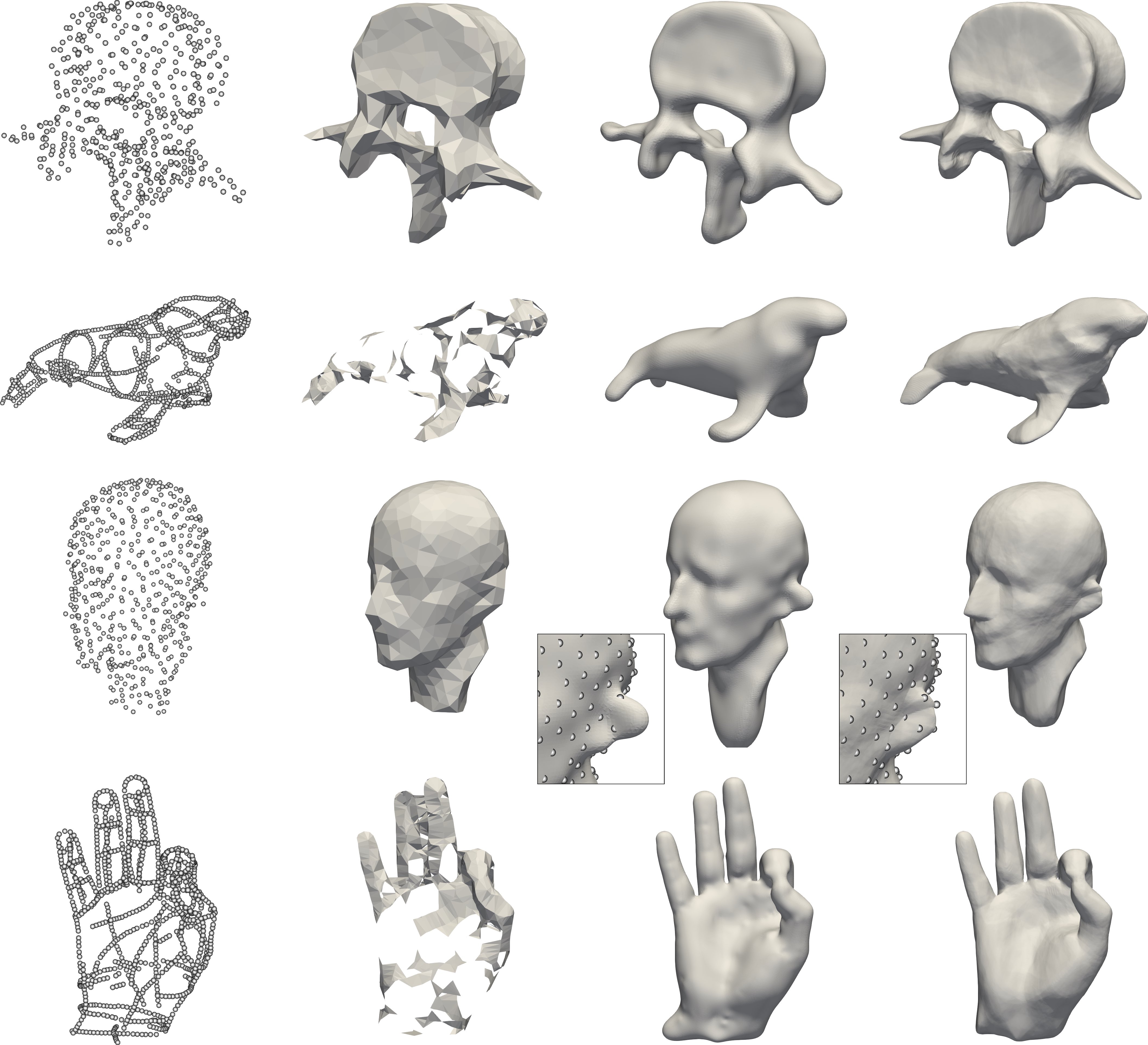
Figure 5: Surface reconstruction from (un-oriented) point cloud. From left to right: input point cloud; ball-pivoting reconstruction [7]; variational-implicit reconstruction [22]; SAL reconstruction (ours).

6.1 Surface reconstruction

The most basic experiment for SAL is reconstructing a surface from a single input raw point cloud (without using any normal information). Figure 5 shows surface reconstructions based on four raw point clouds provided in [22] with three methods: ball-pivoting [7], variation-implicit reconstruction [22], and SAL based on the $L^{0}$ distance, i.e., optimizing the loss described in equation 7 with $\ell=1$. The only parameter in this loss is $\sigma$ which we set for every point in ${\bm{x}}\in{\mathcal{X}}$ to be the distance to the $50$-th nearest point in the point cloud ${\mathcal{X}}$. We used an 8-layer MLP, $f:\mathbb{R}^{3}\times\mathbb{R}^{m}\rightarrow\mathbb{R}$, with 512 wide hidden layers and a single skip connection to the middle layer (see supplementary material for more implementation details). As can be visually inspected from the figure, SAL provides high fidelity surfaces, approximating the input point cloud even for challenging cases of sparse and irregular input point clouds.

6.2 Learning shape space from raw scans

In the main experiment of this paper we trained on the D-Faust scan dataset [8], consisting of approximately 41k raw scans of 10 humans in multiple poses. Each scan is a triangle soup, ${\mathcal{X}}_{i}$, where common defects include holes, ghost geometry, and noise, see Figure 1 for examples.

Architecture.

To learn the shape representations we used a modified variational encoder-decoder [26], where the encoder $({\bm{\mu}},{\bm{\eta}})=g({\bm{X}};{\bm{\theta}}_{1})$ is taken to be PointNet [34] (specific architecture detailed in supplementary material), ${\bm{X}}\in\mathbb{R}^{n\times 3}$ is an input point cloud (we used $n=128^{2}$), ${\bm{\mu}}\in\mathbb{R}^{256}$ is the latent vector, and ${\bm{\eta}}\in\mathbb{R}^{256}$ represents a diagonal covariance matrix by $\bm{\Sigma}=\textrm{diag}\exp{{\bm{\eta}}}$. That is, the encoder takes in a point cloud ${\bm{X}}$ and outputs a probability measure ${\mathcal{N}}({\bm{\mu}},\bm{\Sigma})$. The point cloud is drawn uniformly at random from the scans, i.e., ${\bm{X}}\sim{\mathcal{X}}_{i}$. The decoder is the implicit representation $f({\bm{x}};{\bm{w}},{\bm{\theta}}_{2})$ with the addition of a latent vector ${\bm{w}}\in\mathbb{R}^{256}$. The architecture of $f$ is taken to be the 8-layer MLP, as in Subsection 6.1.

Loss.

We use SAL loss with $L^{2}$ distance, i.e., $h_{2}({\bm{z}})=\min_{{\bm{x}}\in{\mathcal{X}}_{i}}\left\|{\bm{z}}-{\bm{x}}\right\|_{2}$ the unsigned distance to the triangle soup ${\mathcal{X}}_{i}$, and combine it with a variational auto-encoder type loss [26]:

$$\mathrm{Loss}({\bm{\theta}}) =\sum_{i}\mathbb{E}_{{\bm{X}}\sim{\mathcal{X}}_{i}}\Big{[}\mathrm{loss}_{\text{R}}({\bm{\theta}})+\lambda\left\|{\bm{\mu}}\right\|_{1}+\left\|{\bm{\eta}}+\mathbf{1}\right\|_{1}\Big{]}$$

$$\mathrm{loss}_{\text{R}}({\bm{\theta}}) =\mathbb{E}_{{\bm{z}}\sim{\mathcal{N}}_{\sigma}({\mathcal{X}}_{i}),{\bm{w}}\sim{\mathcal{N}}({\bm{\mu}},\bm{\Sigma})}\big{|}|f({\bm{z}};{\bm{w}},{\bm{\theta}}_{2})|-h_{2}({\bm{z}})\big{|},$$

where ${\bm{\theta}}=({\bm{\theta}}_{1},{\bm{\theta}}_{2})$, $\left\|\cdot\right\|_{1}$ is the 1-norm, $\left\|{\bm{\mu}}\right\|_{1}$ encourages the latent prediction ${\bm{\mu}}$ to be close to the origin, while $\left\|{\bm{\eta}}+\mathbf{1}\right\|_{1}$ encourages the variances $\bm{\Sigma}$ to be constant $\exp{(-1)}$; together, these enforce a regularization on the latent space. $\lambda$ is a balancing weight chosen to be $10^{-3}$.

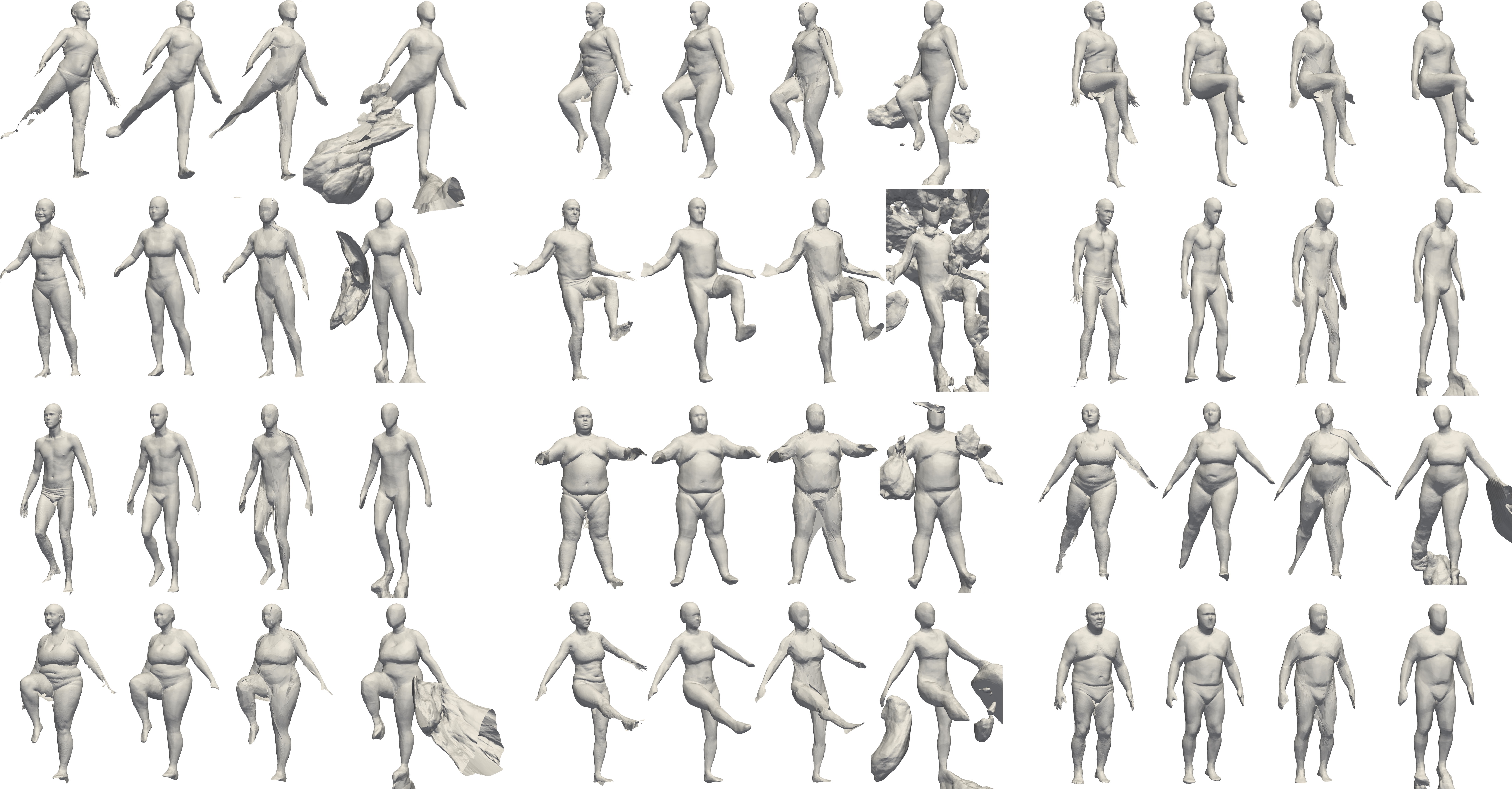
Figure 6: Reconstruction of the test set from D-Faust scans. Left to right in each column: input test scan, SAL (our) reconstruction, AtlasNet [20] reconstruction, and SignReg - signed regression with approximate Jet normals.

Baseline.

We compared versus three baseline methods. First, AtlasNet [20], one of the only existing algorithms for learning a shape collection from raw point clouds. AtlasNet uses a parametric representation of surfaces, which is straight-forward to sample. On the down side, it uses a collection of patches that tend to not overlap perfectly, and their loss requires computation of closest points between the generated and input point clouds which poses a challenge for learning large point clouds. Second, we approximate a signed distance function, $\bar{h}_{2}$, to the data ${\mathcal{X}}_{i}$ in two different ways, and regress them using an MLP as in DeepSDF [32]; we call these methods SignReg. Note that Occupancy Networks [30] and [13] regress a different signed distance function and perform similarly.

To approximate the signed distance function, $\bar{h}_{2}$, we first tried using a state of the art surface reconstruction algorithm [24] to produce watertight manifold surfaces. However, only 28684 shapes were successfully reconstructed ($69\%$ of the dataset), making this option infeasible to compute $\bar{h}_{2}$. We have opted to approximate the signed distance function similar to [21] with $\bar{h}_{2}({\bm{z}})={\bm{n}}_{*}^{T}({\bm{z}}-{\bm{x}}_{*})$, where ${\bm{x}}_{*}=\operatorname*{arg\,min}_{{\bm{x}}\in{\mathcal{X}}_{i}}\left\|{\bm{z}}-{\bm{x}}\right\|_{2}$ is the closest point to ${\bm{z}}$ in ${\mathcal{X}}_{i}$ and ${\bm{n}}_{*}$ is the normal at ${\bm{x}}_{*}\in{\mathcal{X}}_{i}$. To approximate the normal ${\bm{n}}_{*}$ we tested two options: (i) taking ${\bm{n}}^{*}$ directly from the original scan ${\mathcal{X}}_{i}$ with its original orientation; and (ii) using local normal estimation using Jets [11] followed by consistent orientation procedure based on minimal spanning tree using the CGAL library [1].

Table 1 and Figure 6 show the result on a random 75%-25% train-test split on the D-Faust raw scans. We report the 5%, 50% (median), and 95% percentiles of the Chamfer distances between the surface reconstructions and the raw scans (one-sided Chamfer from reconstruction to scan), and ground truth registrations. The SAL and SignReg reconstructions were generated by a forward pass $({\bm{\mu}},{\bm{\eta}})=g({\bm{X}};{\bm{\theta}}_{1})$ of a point cloud ${\bm{X}}\subset{\mathcal{X}}_{i}$ sampled from the raw unseen scans, yielding an implicit function $f({\bm{x}};{\bm{\mu}},{\bm{\theta}}_{2})$. We used the Marching Cubes algorithm [28] to mesh the zero level-set of this implicit function. Then, we sampled uniformly 30K points from it and compute the Chamfer Distance.

Registrations Scans Method 5% Median 95% 5% Median 95% Train AtlasNet[20] 0.09 0.15 0.27 0.05 0.09 0.18 Scan normals 2.53 43.99 292.59 2.63 44.86 257.37 Jet normals 1.72 30.46 513.34 1.65 31.11 453.43 SAL (ours) 0.05 0.09 0.2 0.05 0.06 0.09 Test AtlasNet[20] 0.1 0.17 0.37 0.05 0.1 0.22 Scan normals 3.45 45.03 294.15 3.21 277.36 45.03 Jet normals 1.88 31.05 489.35 1.76 30.89 462.85 SAL (ours) 0.07 0.12 0.35 0.05 0.08 0.16

Table 1: Reconstruction of the test set from D-Faust scans. We log the Chamfer distances of the reconstructed surfaces to the raw scans (one-sided), and ground-truth registrations; we report the 5-th, 50-th, and 95-th percentile. Numbers are reported $*10^{3}$.

Generalization to unseen data.

In this experiment we test our method on two different scenarios: (i) generating shapes of unseen humans; and (ii) generating shapes of unseen poses. For the unseen humans experiment we trained on $8$ humans ($4$ females and $4$ males), leaving out $2$ humans for test (one female and one male). For the unseen poses experiment, we randomly chose two poses of each human as a test set. To further improve test-time shape representations, we also further optimized the latent ${\bm{\mu}}$ to better approximate the input test scan ${\mathcal{X}}_{i}$. That is, for each test scan ${\mathcal{X}}_{i}$, after the forward pass $({\bm{\mu}},{\bm{\eta}})=g({\bm{X}};{\bm{\theta}}_{2})$ with ${\bm{X}}\subset{\mathcal{X}}_{i}$, we further optimized $\mathrm{loss}_{\text{R}}$ as a function of ${\bm{\mu}}$ for 800 further iterations. We refer to this method as latent optimization.

Table 2 demonstrates that the latent optimization method further improves predictions quality, compared to a single forward pass. In 7 and 8, we demonstrate few representatives examples, where we plot left to right in each column: input test scan, SAL reconstruction with forward pass alone, and SAL reconstruction with latent optimization. Failure cases are shown in the bottom-right. Despite the little variability of humans in the training dataset (only 8 humans), 7 shows that SAL can usually fit a pretty good human shape to the unseen human scan using a single forward pass reconstruction; using latent optimization further improves the approximation as can be inspected in the different examples in this figure.

Figure 8 shows how a single forward reconstruction is able to predict the pose correctly, where latent optimization improves the prediction in terms of shape and pose.

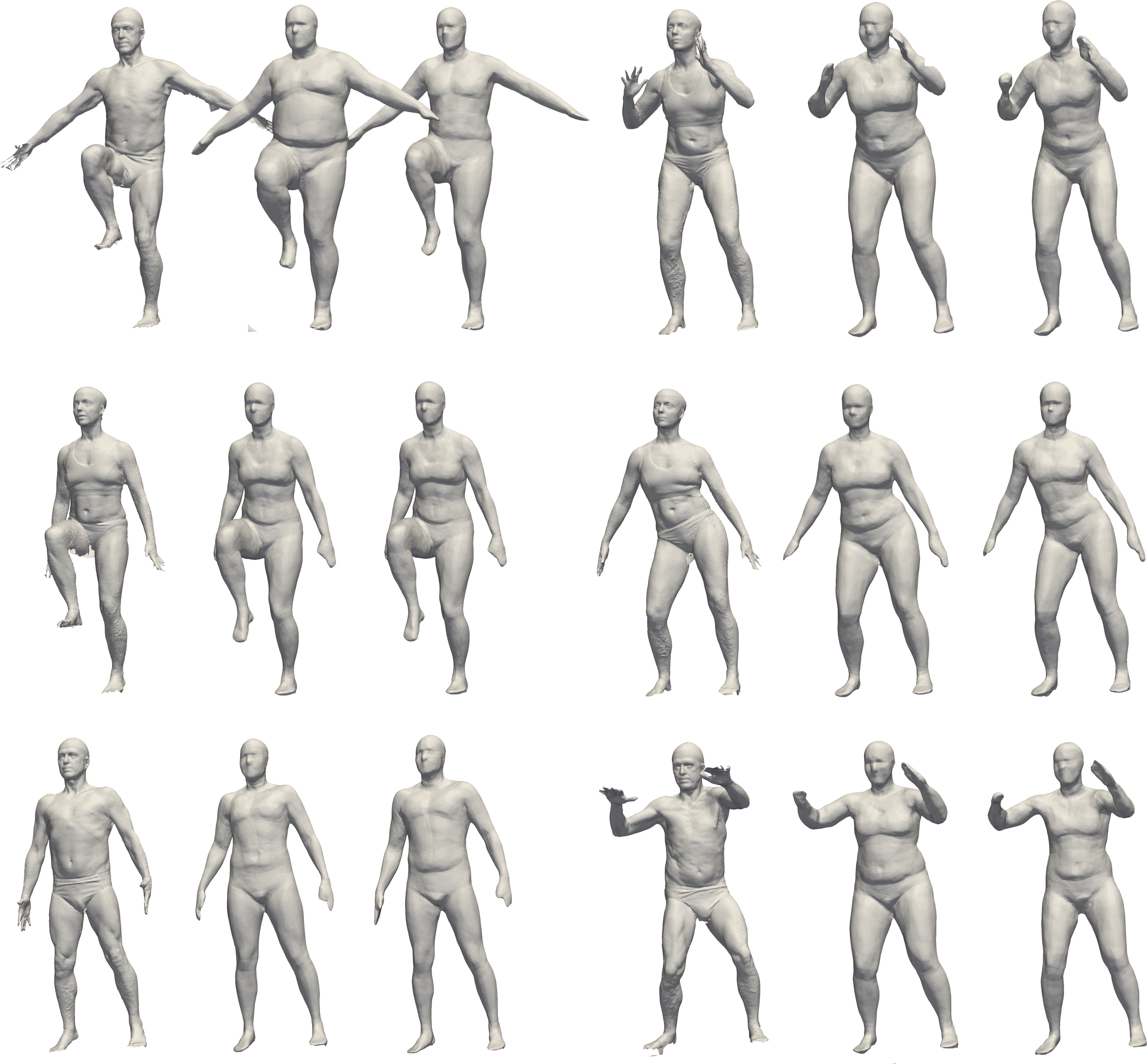
Figure 7: Reconstruction of unseen humans scans. Each column from left to right: unseen human scan, SAL reconstruction with a single forward pass, SAL reconstruction with latent optimization. Bottom-right shows failure.

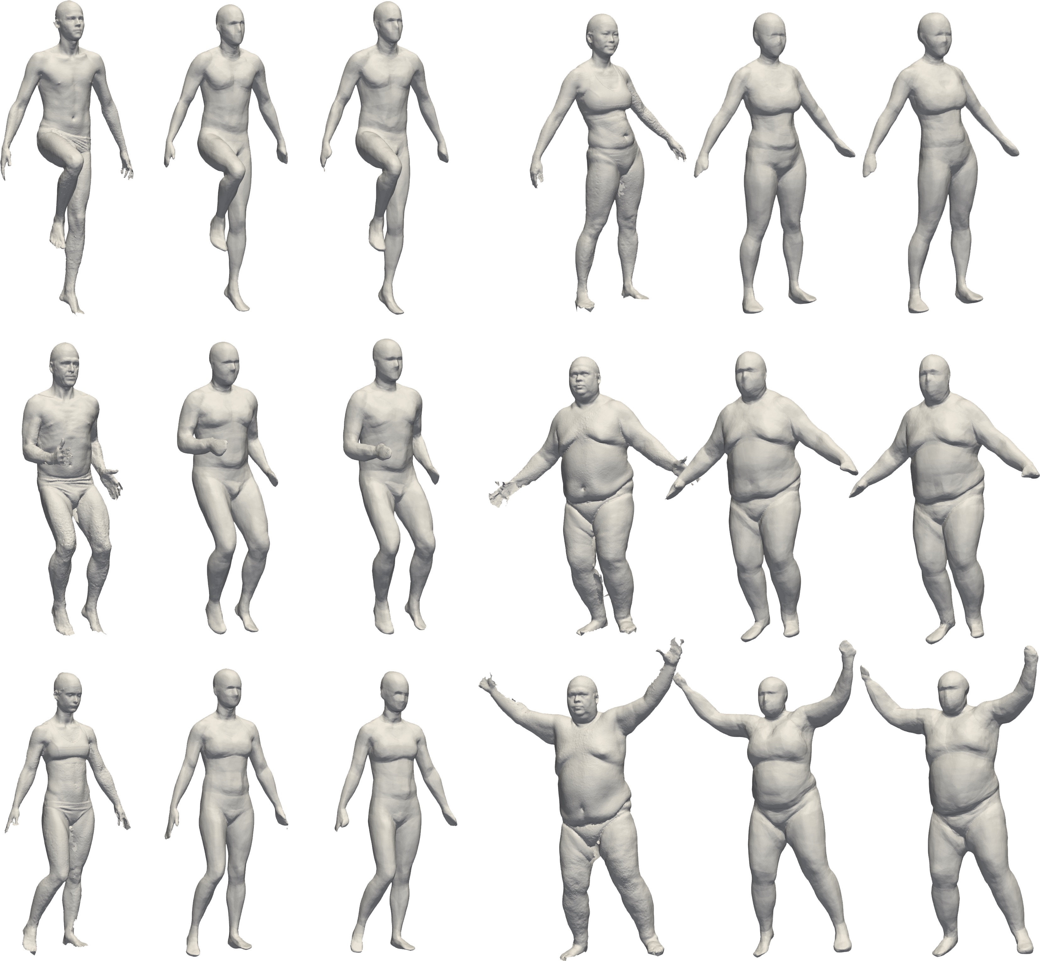
Figure 8: Reconstruction of unseen pose scans. Each column from left to right: unseen pose scan, SAL reconstruction with a single forward pass, SAL reconstruction with latent optimization. Bottom-right shows failure.

Registrations Scans Method 5% Median 95% 5% Median 95% Train SAL (Pose) 0.08 0.12 0.25 0.05 0.07 0.1 SAL (Human) 0.06 0.09 0.18 0.04 0.06 0.09 Test SAL (Pose) 0.11 0.37 2.26 0.07 0.18 0.93 SAL + latent opt. (Pose) 0.08 0.16 1.12 0.05 0.09 0.19 SAL (Human) 0.26 0.75 4.99 0.14 0.34 1.53 SAL + latent opt. (Human) 0.12 0.3 3.05 0.07 0.14 0.49

Table 2: Reconstruction of the unseen human and pose from D-Faust scans. We log the Chamfer distances of the reconstructed surfaces to the raw scans (one-sided), and ground-truth registrations; we report the 5-th, 50-th, and 95-th percentile. Numbers are reported $*10^{3}$.

Limitations.

SAL’s limitation is mainly in capturing thin structures. Figure 9 shows reconstructions (obtained similarly to 6.1) of a chair and a plane from the ShapeNet [12] dataset; note that some parts in the chair back and the plane wheel structure are missing.

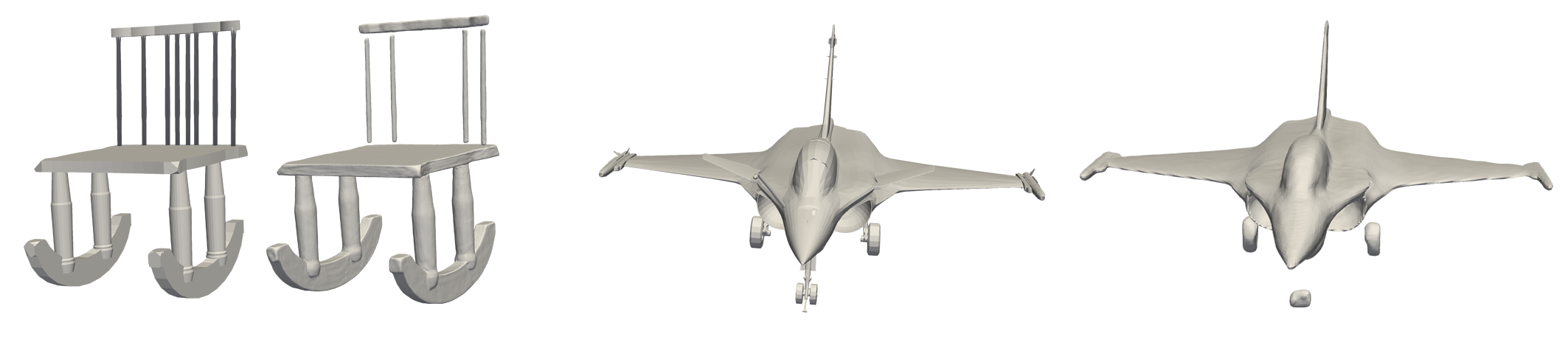
Figure 9: Failure in capturing thin structures. In each pair: ground truth model (left), and SAL reconstruction (right).

7 Conclusions

We introduced SAL: Sign Agnostic Learning, a deep learning approach for processing raw data without any preprocess or need for ground truth normal data or inside/outside labeling. We have developed a geometric initialization formula for MLPs to approximate the signed distance function to a sphere, and a theoretical justification proving planar reproduction for SAL. Lastly, we demonstrated the ability of SAL to reconstruct high fidelity surfaces from raw point clouds, and that SAL easily integrates into standard generative models to learn shape spaces from raw geometric data. One limitation of SAL was mentioned in Section 5, namely the stopping criteria for the optimization.

Using SAL in other generative models such as generative adversarial networks could be an interesting follow-up. Another future direction is global reconstruction from partial data. Combining SAL with image data also has potentially interesting applications. We think SAL has many exciting future work directions, progressing geometric deep learning to work with unorganized, raw data.

Acknowledgments

The research was supported by the European Research Council (ERC Consolidator Grant, ”LiftMatch” 771136), the Israel Science Foundation (Grant No. 1830/17) and by a research grant from the Carolito Stiftung (WAIC).

8 Appendix

8.1 Implementation details

8.1.1 Surface reconstruction

Data Preparation.

For each point cloud ${\mathcal{X}}\subset\mathbb{R}^{3}$ we created training data by sampling two Gaussian variables centered at each ${\bm{x}}\in{\mathcal{X}}$. We set the standard deviation of the first Gaussian to be the distance to the 50-th closest point in ${\mathcal{X}}$, whereas the second Gaussian standard deviation is set to be the distance to the furthest point in ${\mathcal{X}}$.

Network Architecture.

We use an MLP as detailed in equation 8 and equation 9 with $\ell=7$, i.e., 8 layers, where $d_{i}^{out},d_{i}^{in}=512$ for interior layers and $d_{1}^{in}=3$. We also add a skip connection at the 4-th layer concatenating the input point ${\bm{x}}\in\mathbb{R}^{3}$ with the hidden variable ${\bm{y}}\in\mathbb{R}^{509}$, i.e., $[{\bm{x}},{\bm{y}}]\in\mathbb{R}^{512}$, where accordingly $d_{3}^{out}=509$.

Training Details.

We train the network in the surface reconstruction experiment with Adam optimizer [25], learning rate $0.0001$ for 5000 epochs. Training was done on an Nvidia V-100 GPU, using pytorch deep learning framework [33].

8.1.2 Learning shape space

Data Preparation.

To speed up training on the D-Faust dataset, we preprocessed the original scans ${\mathcal{X}}\subset\mathbb{R}^{3}$ and sampled 500K points from each scan. The size of the sample is similar to [32]. First, we sampled 250K points uniformly (w.r.t. area) from the triangle soup ${\mathcal{X}}$ and then placed two Gaussian random variables centered at each sample point ${\bm{x}}\in{\mathcal{X}}$. We set the standard deviation of the first Gaussian to be the distance to the 50-th closest point in ${\mathcal{X}}$, whereas the second Gaussian standard deviation is set to be $0.2$. For each sample point we calculated its unsigned distance to the closest triangle in the triangle soup. The distance computation was done using [1].

Network Architecture.

Our network architecture is Encoder-Decoder based, where for the encoder we have used PointNet [34] and DeepSets [46] layers. Each layer is composed of

$$\mathrm{PFC}(d_{\text{in}},d_{\text{out}}):{\bm{X}} \mapsto\nu\left({\bm{X}}W+\mathbf{1}b^{T}\right)$$

$$\mathrm{PL}(d_{\text{in}},2d_{\text{in}}):{\bm{Y}} \mapsto\left[{\bm{Y}},\max{({\bm{Y}})}\mathbf{1}\right]$$

where $\left[\cdot,\cdot\right]$ is the concat operation. Our Architecture is

$$\mathrm{PFC}(3,128)\rightarrow\mathrm{PFC}(128,128)\rightarrow\mathrm{PL}(128,256)\rightarrow$$

$$\mathrm{PFC}(256,128)\rightarrow\mathrm{PL}(128,256)\rightarrow\mathrm{PFC}(256,128)\rightarrow$$

$$\mathrm{PL}(128,256)\rightarrow\mathrm{PFC}(256,128)\rightarrow\mathrm{PL}(128,256)\rightarrow$$

$$\mathrm{PFC}(256,256)\rightarrow\mathrm{MaxPool}\rightarrow\mathrm{FC}(256,256),$$

similarly to [30] SimplePointNet architecture. For the decoder, our network architecture is the same as in the Surface reconstruction experiment except for $d_{1}^{in}=256+3$, as the decoder receives as input $\left[z,x\right]\in\mathbb{R}^{259}$. Where $\left[z,x\right]$ is a concatenation of the latent encoding ${\bm{z}}\in\mathbb{R}^{256}$ and a point ${\bm{x}}\in\mathbb{R}^{3}$ in space.

Training Details.

Training our networks for learning the shape space of the D-Faust dataset was done with the following choices. We have used the Adam optimizer [25], initialized with learning rate $0.0005$ and batch size of $64$. We scheduled the learning rate to decrease every 500 epochs by a factor of 0.5. We stopped the training process after 2000 epochs. Training was done on 4 Nvidia V-100 GPUs, using pytorch deep learning framework [33].

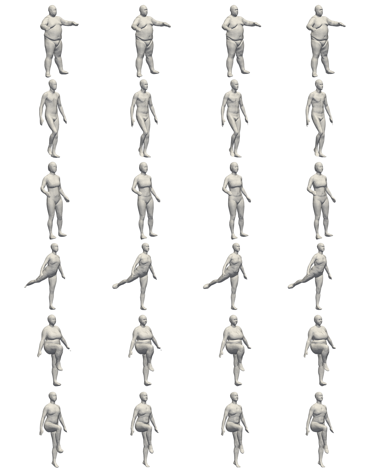
Figure 10: Effect of the number of training epochs on reconstruction quality of test scans. Left to right in each row: epoch $500$, $1500$, $2500$ and $3500$.

8.2 Additional Experiments

Single reconstruction versus VAE reconstruction.

One of the key advantages of SAL is that it can be used for reconstructing a surface from a single input scan or incorporated into a VAE architecture for learning a shape space from an entire scans dataset. This raises an interesting question, whether learning a shape space has also an impact on the quality of the reconstructions. To answer this question, we ran SAL surface reconstruction on each of the scans used for training the main experiment of the paper (See table 2 for more details). When comparing our SAL VAE training results on the registrations (ground truth) versus SAL single reconstruction we see differences in favor of our VAE learner, whereas the results on the original scans are comparable. That is, SAL single reconstruction results are $0.10,0.17,0.22;0.07,0.08,0.10$ on the registrations and scans for the $5\%,50\%,95\%$ percentiles respectively.

Number of epochs used for training SAL VAE.

Figure 10 shows reconstructions of test scans for different stages of training on the D-Faust dataset. Given the main paper discussion on SAL limit signed function, we additionally add reconstructions from relatively advanced epoch as $3500$, showing that no error in contouring occur.

8.3 Proofs

8.3.1 Proof of Theorem 3

Theorem 3.

Consider a linear model $f({\bm{x}};{\bm{\theta}})=\varphi({\bm{w}}^{T}{\bm{x}}+b)$, ${\bm{\theta}}=({\bm{w}},b)$, with a strong non-linearity $\varphi:\mathbb{R}\rightarrow\mathbb{R}$. Assume the data ${\mathcal{X}}$ lies on a plane ${\mathcal{P}}=\left\{{\bm{x}}|{\bm{n}}^{T}{\bm{x}}+c=0\right\}$, i.e., ${\mathcal{X}}\subset{\mathcal{P}}$. Then, there exists $\alpha\in\mathbb{R}_{+}$ so that $({\bm{w}}^{*},b^{*})=(\alpha{\bm{n}},\alpha c)$ is a critical point of the loss in equation 2.

Proof.

For simplicity, we restrict our attention to absolutely continuous measures $D_{\mathcal{X}}$, that is defined by a continuous density function $\mu({\bm{x}})$. Generalizing to measures with a discrete part (such as the one we use for the $L^{0}$ distance, for example) can be proven similarly.

Denoting ${\bm{\theta}}=({\bm{w}},b)$, the loss in equation 2 can be written as

$$\mathrm{loss}({\bm{w}},b)=\int_{\mathbb{R}^{d}}\tau(f({\bm{x}};{\bm{\theta}}),h_{\mathcal{X}}({\bm{x}}))\mu({\bm{x}})d{\bm{x}}.$$

Denote by ${\bm{r}}:\mathbb{R}^{d}\rightarrow\mathbb{R}^{d}$ the linear reflection w.r.t. ${\mathcal{P}}$, i.e., ${\bm{r}}({\bm{x}})={\bm{x}}-2{\bm{n}}{\bm{n}}^{T}({\bm{x}}-{\bm{x}}_{0})=(I-2{\bm{n}}{\bm{n}}^{T}){\bm{x}}-2c{\bm{n}}$, where ${\bm{x}}_{0}\in{\mathcal{P}}$ is an arbitrary point. $h_{\mathcal{X}}$ and $\mu$ are invariant to ${\bm{r}}$, that is $h_{\mathcal{X}}({\bm{r}}({\bm{x}}))=h_{\mathcal{X}}({\bm{x}})$, $\mu({\bm{r}}({\bm{x}}))=\mu({\bm{x}})$.

The gradient of the loss is $\nabla_{{\bm{w}},b}\mathrm{loss}({\bm{w}},b)=$

$$\int_{\mathbb{R}^{d}}\frac{\partial\tau}{\partial a}(f({\bm{x}};{\bm{\theta}}),h_{\mathcal{X}}({\bm{x}}))\nabla_{{\bm{w}},b}f({\bm{x}};{\bm{\theta}})\mu({\bm{x}})d{\bm{x}},$$ (10)

where $\nabla_{{\bm{w}},b}f({\bm{x}};{\bm{\theta}})=\varphi^{\prime}({\bm{w}}^{T}{\bm{x}}+b)[{\bm{x}},1]$.

Let ${\bm{w}}=\alpha{\bm{n}}$ and $b=\alpha c$, where $\alpha\in\mathbb{R}_{+}$ is currently arbitrary. We decompose $\mathbb{R}^{d}$ to the two sides of ${\mathcal{P}}$, $\Omega_{+}=\left\{{\bm{x}}|{\bm{n}}^{T}{\bm{x}}+c\geq 0\right\}$, and $\Omega_{-}=\mathbb{R}^{d}\setminus\Omega_{+}$. Now consider the integral in equation 10 restricted to $\Omega_{-}$ and perform change of variables ${\bm{x}}={\bm{r}}({\bm{y}})$; note that ${\bm{r}}$ consists of an orthogonal linear part and therefore $d{\bm{y}}=\left|\det\frac{\partial{\bm{y}}}{\partial{\bm{x}}}\right|d{\bm{x}}=d{\bm{x}}$. Furthermore, property (i) implies that $\frac{\partial\tau}{\partial a}(a,b)=-\frac{\partial\tau}{\partial a}(-a,b)$, and since $\varphi$ is anti-symmetric and ${\bm{w}}^{T}{\bm{r}}({\bm{x}})+b=-({\bm{w}}^{T}{\bm{y}}+b)$ we get

$$\frac{\partial\tau}{\partial a}(f({\bm{r}}({\bm{y}});{\bm{\theta}}),h_{\mathcal{X}}({\bm{r}}({\bm{y}})))=-\frac{\partial\tau}{\partial a}(f({\bm{y}};{\bm{\theta}}),h_{\mathcal{X}}({\bm{y}})).$$

As $\varphi$ is anti-symmetric, $\varphi^{\prime}$ is symmetric, i.e., $\varphi^{\prime}(a)=\varphi^{\prime}(-a)$ and therefore

$$\varphi^{\prime}({\bm{w}}^{T}{\bm{r}}({\bm{y}})+b)=\varphi^{\prime}({\bm{w}}^{T}{\bm{y}}+b).$$

Plugging these in the integral after the change of variables we reach

$$-\int_{\Omega_{+}}\frac{\partial\tau}{\partial a}(f({\bm{y}};{\bm{\theta}}),h_{\mathcal{X}}({\bm{y}}))\varphi^{\prime}({\bm{w}}^{T}{\bm{y}}+b)[{\bm{r}}({\bm{y}}),1]\mu({\bm{y}})d{\bm{y}}.$$

An immediate consequence is that $\nabla_{b}\mathrm{loss}({\bm{w}},b)=0$. As for $\nabla_{\bm{w}}\mathrm{loss}({\bm{w}},b)$ we have:

$$\int_{\Omega_{+}}\frac{\partial\tau}{\partial a}(f({\bm{x}};{\bm{\theta}}),h_{\mathcal{X}}({\bm{x}}))\varphi^{\prime}({\bm{w}}^{T}{\bm{x}}+b)({\bm{x}}-{\bm{r}}({\bm{x}}))\mu({\bm{x}})d{\bm{x}}.$$

Since ${\bm{x}}-{\bm{r}}({\bm{x}})=2{\bm{n}}{\bm{n}}^{T}({\bm{x}}-{\bm{x}}_{0})$ we get $\nabla_{\bm{w}}\mathrm{loss}({\bm{w}},b)=$

$$2{\bm{n}}\int_{\Omega_{+}}\frac{\partial\tau}{\partial a}(f({\bm{x}};{\bm{\theta}}),h_{\mathcal{X}}({\bm{x}}))\varphi^{\prime}({\bm{w}}^{T}{\bm{x}}+b){\bm{n}}^{T}({\bm{x}}-{\bm{x}}_{0})\mu({\bm{x}})d{\bm{x}}.$$

The last integral is scalar and we denote its integrand by $g_{\alpha}({\bm{x}})$ (remember that $({\bm{w}},b)=\alpha({\bm{n}},c)$), i.e.,

$$\nabla_{\bm{w}}\mathrm{loss}({\bm{w}},b)=2{\bm{n}}\int_{\Omega_{+}}g_{\alpha}({\bm{x}})d{\bm{x}}=2{\bm{n}}G(\alpha),$$

where $G(\alpha)=\int_{\Omega_{+}}g_{\alpha}({\bm{x}})d{\bm{x}}$. The proof will be done if we show there exists $\alpha\in\mathbb{R}_{+}$ so that $G(\alpha)=0$. We will use the intermediate value theorem for continuous functions to prove this, that is, we will show existence of $\alpha_{-},\alpha_{+}\in\mathbb{R}_{+}$ so that $G(\alpha_{-})<0<G(\alpha_{+})$.

Let us show the existence of $\alpha_{+}$. Let ${\bm{x}}\in\Omega_{+}$ such that $\gamma={\bm{n}}^{T}{\bm{x}}+c>0$ and $\mu({\bm{x}})>0$. Then,

$$g_{\alpha}({\bm{x}})=\frac{\partial\tau}{\partial a}(\varphi(\alpha\gamma),h_{\mathcal{X}}({\bm{x}}))\varphi^{\prime}(\alpha\gamma)\gamma\mu({\bm{x}}).$$

Furthermore, since $\beta^{-1}\geq\varphi^{\prime}(a)\geq\beta>0$ we have that

$$g_{\alpha}({\bm{x}}) \geq\frac{\partial\tau}{\partial a}(\varphi(\alpha\gamma),h_{\mathcal{X}}({\bm{x}}))\gamma\mu({\bm{x}})\begin{cases}\beta&\frac{\partial\tau}{\partial a}\geq 0\\ \beta^{-1}&\frac{\partial\tau}{\partial a}<0\end{cases}$$

$$=\tilde{g}_{\alpha}({\bm{x}}).$$

Note that $\tilde{g}_{\alpha}({\bm{x}})$ is monotonically increasing and for sufficiently large $\alpha\in\mathbb{R}_{+}$ we have that $\tilde{g}_{\alpha}({\bm{x}})>0$. Since $\int_{\Omega_{+}}\tilde{g}_{\alpha}({\bm{x}})d{\bm{x}}>-\infty$ for all $\alpha\in\mathbb{R}_{+}$ the integral monotone convergence theorem implies that $\lim_{\alpha\rightarrow\infty}\int_{\Omega_{+}}\tilde{g}_{\alpha}({\bm{x}})d{\bm{x}}>0$. Lastly, since

$$\int_{\Omega_{+}}g_{\alpha}({\bm{x}})d{\bm{x}}\geq\int_{\Omega_{+}}\tilde{g}_{\alpha}({\bm{x}})d{\bm{x}},$$

the existence of $\alpha_{+}$ is established. The case of $\alpha_{-}$ is proven similarly. ∎

8.3.2 Local plane reproduction with MLP

Theorem 4.

Consider an MLP as defined in equation 8. Assume that locally in some domain $\Omega\subset\mathbb{R}^{d}$ the data ${\mathcal{X}}\cap\Omega$ lies on a plane ${\mathcal{P}}=\left\{{\bm{x}}|{\bm{n}}^{T}{\bm{x}}+c=0\right\}$, i.e., ${\mathcal{X}}\cap\Omega\subset{\mathcal{P}}$. Then, there exists a critical point ${\bm{\theta}}^{*}$ of the loss in equation 2 that reconstructs ${\mathcal{P}}$ locally in $\Omega$.

By ”reconstructs ${\mathcal{P}}$ locally” we mean that ${\bm{\theta}}^{*}$ is critical for the loss if $D_{\mathcal{X}}$ is sufficiently concentrated around any point in ${\mathcal{P}}\cap\Omega$.

Proof.

We next consider a general MLP model $f({\bm{x}};{\bm{\theta}})$ as in equation 8. We denote by $\mathrm{supp}(\mu)$ the support set of $\mu$, i.e., $\left\{{\bm{x}}|\mu({\bm{x}})>0\right\}$. Let us write the layers of the network $f({\bm{x}};{\bm{\theta}})$ using only matrix multiplication, that is

$$f_{i}({\bm{y}})=\textrm{diag}\big{(}H({\bm{W}}_{i}{\bm{y}}+{\bm{b}}_{i})\big{)}\big{(}{\bm{W}}_{i}{\bm{y}}+{\bm{b}}_{i}\big{)},$$ (11)

where $H(a)={\tiny\begin{cases}1&a\geq 0\\ 0&a<0\end{cases}}$ is the Heaviside function.

Let $\mu$ be so that $\mathrm{supp}(\mu)\subset\Omega$, and fix an arbitrary ${\bm{x}}_{0}\in\mathrm{supp}(\mu)\cap{\mathcal{P}}$. Next, let ${\bm{\theta}}\in\mathbb{R}^{m}$ be such that: (a) there exists a domain $\Upsilon$, so that $\mathrm{supp}(\mu)\subset\Upsilon$ and for which all the diagonal matrices in equation 11 are constants, i.e., $\Upsilon$ is a domain over which $f({\bm{x}};{\bm{\theta}})$ (excluding the final non-linearity $\varphi$) is linear as a function of ${\bm{x}}$. Therefore, for ${\bm{x}}\in\Upsilon$ we have the layers of $f$ satisfy

$$f_{i}({\bm{y}})=D_{i}\big{(}{\bm{W}}_{i}{\bm{y}}+{\bm{b}}_{i}\big{)},$$

and $D_{i}$ are constant diagonal matrices. Over this domain we have

$$f({\bm{x}};{\bm{\theta}})=\varphi\big{(}{\bm{w}}({\bm{\theta}})^{T}{\bm{x}}+b({\bm{\theta}})\big{)},$$

and therefore

$$\nabla_{\bm{\theta}}f({\bm{x}};{\bm{\theta}})={\bm{A}}\nabla_{{\bm{w}},b}f({\bm{x}};{\bm{\theta}}),$$ (12)

where $\nabla_{{\bm{w}},b}f({\bm{x}};{\bm{\theta}})=\varphi^{\prime}({\bm{w}}({\bm{\theta}})^{T}{\bm{x}}+b({\bm{\theta}}))[{\bm{x}},1]$, and ${\bm{A}}\in\mathbb{R}^{m\times(d+1)}$ is a matrix holding the partial derivatives of ${\bm{w}}({\bm{\theta}})$ and $b({\bm{\theta}})$. (b) over $\Upsilon$ there exists ${\bm{w}}({\bm{\theta}})={\bm{n}}$ and $b({\bm{\theta}})=c$. The existence of such ${\bm{\theta}}$ is guaranteed for example from Theorem 2.1 in [2].

Similarly to the proof of Theorem 3 there exists $\alpha\in\mathbb{R}_{+}$ so that $\nabla_{{\bm{w}},b}\mathrm{loss}(\alpha{\bm{w}}({\bm{\theta}}),\alpha b({\bm{\theta}}))=0$. Scaling the ${\bm{w}},b$ components of ${\bm{\theta}}$ by $\alpha$ and denoting the new parameter vector by ${\bm{\theta}}^{*}$, we get that $\nabla_{{\bm{w}},b}\mathrm{loss}({\bm{w}}({\bm{\theta}}^{*}),b({\bm{\theta}}^{*}))=0$ (see equation 10) and therefore equation 12 implies that $\nabla_{\bm{\theta}}\mathrm{loss}({\bm{\theta}}^{*})=0$, as required. ∎

8.3.3 Proof of Theorem 1

Theorem 1.

Let $f$ be an MLP (see equations 8-9). Set, for $1\leq i\leq\ell$, ${\bm{b}}_{i}=0$ and ${\bm{W}}_{i}$ i.i.d. from a normal distribution ${\mathcal{N}}(0,\frac{\sqrt{2}}{\sqrt{d_{i}^{out}}})$; further set ${\bm{w}}={\frac{\sqrt{\pi}}{\sqrt{d_{\ell}^{out}}}}\mathbf{1}$, $c=-r$. Then, $f({\bm{x}})\approx\varphi(\left\|x\right\|-r)$.

Proof.

To prove this theorem reduce the problem to a single hidden layer network, see Theorem 2. Denote $g({\bm{x}})=f_{\ell-1}\circ\cdots\circ f_{1}$. If we prove that $\left\|g({\bm{x}})\right\|\approx\left\|{\bm{x}}\right\|$ then Theorem 2 implies the current theorem.

It is enough to consider a single layer: $h({\bm{x}})=\nu({\bm{W}}{\bm{x}}+{\bm{b}})$. For brevity let $k=d^{out}$. Now,

$$\left\|h({\bm{x}})\right\|^{2}=\sum_{i=1}^{k}\nu({\bm{W}}_{i,:}\cdot{\bm{x}})^{2}=\frac{1}{k}\sum_{i=1}^{k}\nu(\sqrt{k}{\bm{W}}_{i,:}\cdot{\bm{x}})^{2}.$$

Note that the entries of $\sqrt{k{\bm{W}}_{i,:}}$ are distributed i.i.d. ${\mathcal{N}}(0,\sqrt{2})$. Hence by the law of large numbers the last term converge to

$$\left\|{\bm{x}}\right\|^{2}\int_{\mathbb{R}^{k}}\nu\left({\bm{y}}\cdot\frac{{\bm{x}}}{\left\|{\bm{x}}\right\|}\right)^{2}\mu({\bm{y}})dy$$

$$=\left\|{\bm{x}}\right\|^{2}\int_{\mathbb{R}^{k}}\nu(y_{1})^{2}\frac{1}{(2\pi\sigma^{2})^{k/2}}e^{-\frac{\left\|{\bm{y}}\right\|}{2\sigma^{2}}}dy$$

$$=\left\|{\bm{x}}\right\|^{2}\int_{\mathbb{R}}\nu(y_{1})^{2}\frac{1}{\sqrt{2\pi\sigma^{2}}}e^{-\frac{y_{1}^{2}}{2\sigma^{2}}}dy$$

$$=\frac{\left\|{\bm{x}}\right\|^{2}}{2}\int_{\mathbb{R}}y_{1}^{2}\frac{1}{\sqrt{2\pi\sigma^{2}}}e^{-\frac{y_{1}^{2}}{2\sigma^{2}}}dy$$

$$=\left\|{\bm{x}}\right\|^{2},$$

where in the second equality, similarly to the proof of Theorem 2, we changed variables, ${\bm{y}}={\bm{R}}{\bm{y}}^{\prime}$, where we chose ${\bm{R}}\in\mathbb{R}^{k\times k}$ orthogonal so that ${\bm{R}}^{T}\frac{{\bm{x}}}{\left\|{\bm{x}}\right\|}=(1,0,\ldots,0)^{T}$. ∎

Skip connections.

Adapting the geometric initialization to skip connections is easy: consider skip connection layers of the form $s({\bm{y}})=\frac{1}{\sqrt{2}}({\bm{y}},{\bm{x}})$, where ${\bm{x}}\in\mathbb{R}^{d}$ is the input to the network and ${\bm{y}}\in\mathbb{R}^{d^{out}_{i}}$ is some interior hidden variable. Then $\left\|s({\bm{y}})\right\|^{2}=\frac{1}{2}\left\|{\bm{x}}\right\|^{2}+\frac{1}{2}\left\|{\bm{y}}\right\|^{2}$. According to Theorem 1 we have $\left\|{\bm{y}}\right\|\approx\left\|{\bm{x}}\right\|$ and hence $\left\|s({\bm{y}})\right\|^{2}\approx\left\|{\bm{x}}\right\|^{2}$.

8.3.4 Proof of Theorem 2

Theorem 2.

Let $f:\mathbb{R}^{d}\rightarrow\mathbb{R}$ be an MLP with ReLU activation, $\nu$, and a single hidden layer. That is, $f({\bm{x}})={\bm{w}}^{T}\nu({\bm{W}}{\bm{x}}+{\bm{b}})+c$, where ${\bm{W}}\in\mathbb{R}^{d^{out}\times d}$, ${\bm{b}}\in\mathbb{R}^{d^{out}}$, ${\bm{w}}\in\mathbb{R}^{d^{out}}$, $c\in\mathbb{R}$ are the learnable parameters. If ${\bm{b}}=0$, ${\bm{w}}=\frac{\sqrt{2\pi}}{\sigma d^{out}}\mathbf{1}$, $c=-r$, $r>0$, and all entries of ${\bm{W}}$ are i.i.d. normal ${\mathcal{N}}(0,\sigma^{2})$ then $f({\bm{x}})\approx\left\|{\bm{x}}\right\|-r$. That is, $f$ is approximately the signed distance function to a $d-1$ sphere of radius $r$ in $\mathbb{R}^{d}$, centered at the origin.

Proof.

For brevity we denote $k=d^{out}$. Note that plugging ${\bm{w}},{\bm{b}},c$ in $f$ we get $f({\bm{x}})=\frac{\sqrt{2\pi}}{\sigma k}\sum_{i=1}^{k}\nu({\bm{w}}_{i}\cdot{\bm{x}})-r$, where ${\bm{w}}_{i}$ is the $i^{th}$ row of ${\bm{W}}$. Let $\mu$ denote the density of multivariate normal distribution ${\mathcal{N}}=(0,\sigma^{2}I_{k})$. By the law of large numbers, the first term converges to

$$\frac{\sqrt{2\pi}}{\sigma}\int_{\mathbb{R}^{k}}\nu\left({\bm{u}}\cdot\frac{{\bm{x}}}{\left\|{\bm{x}}\right\|}\left\|{\bm{x}}\right\|\right)\mu({\bm{u}})d{\bm{u}}$$

$$=\frac{\sqrt{2\pi}\left\|{\bm{x}}\right\|}{\sigma}\int_{\mathbb{R}^{k}}\nu\left({\bm{u}}\cdot\frac{{\bm{x}}}{\left\|{\bm{x}}\right\|}\right)\mu({\bm{u}})d{\bm{u}}$$

$$=\frac{\sqrt{2\pi}\left\|{\bm{x}}\right\|}{\sigma}\int_{\mathbb{R}^{k}}\nu(v_{1})\mu({\bm{v}})d{\bm{v}}$$

$$=\frac{\sqrt{2\pi}\left\|{\bm{x}}\right\|}{\sigma}\int_{\mathbb{R}^{k}}\nu(v_{1})\frac{1}{(2\pi\sigma^{2})^{k/2}}e^{-\frac{\left\|{\bm{v}}\right\|^{2}}{2\sigma^{2}}}d{\bm{v}}$$

$$=\frac{\sqrt{2\pi}\left\|{\bm{x}}\right\|}{\sigma}\int_{\mathbb{R}}\nu(v_{1})\frac{1}{\sqrt{2\pi\sigma^{2}}}e^{-\frac{v_{1}^{2}}{2\sigma^{2}}}dv_{1}$$

$$=\frac{\sqrt{2\pi}\left\|{\bm{x}}\right\|}{2\sigma}\int_{\mathbb{R}}\left|v_{1}\right|\frac{1}{\sqrt{2\pi\sigma^{2}}}e^{-\frac{v_{1}^{2}}{2\sigma^{2}}}dv_{1}$$

$$=\left\|{\bm{x}}\right\|,$$

where in the second equality we changed variables, ${\bm{u}}={\bm{R}}{\bm{v}}$, where we chose ${\bm{R}}\in\mathbb{R}^{k\times k}$ orthogonal so that ${\bm{R}}^{T}\frac{{\bm{x}}}{\left\|{\bm{x}}\right\|}=(1,0,\ldots,0)^{T}$, and used the rotation invariance of $\mu$, namely $\mu({\bm{R}}{\bm{v}})=\mu({\bm{v}})$. In the last equality we used the mean of the folded normal distribution. Therefore we get $f({\bm{x}})\approx{\left\|{\bm{x}}\right\|-r}$. ∎

References

- [1] Pierre Alliez, Simon Giraudot, Clément Jamin, Florent Lafarge, Quentin Mérigot, Jocelyn Meyron, Laurent Saboret, Nader Salman, and Shihao Wu. Point set processing. In CGAL User and Reference Manual. CGAL Editorial Board, 5.0 edition, 2019.
- [2] Raman Arora, Amitabh Basu, Poorya Mianjy, and Anirbit Mukherjee. Understanding deep neural networks with rectified linear units. arXiv preprint arXiv:1611.01491, 2016.
- [3] Matan Atzmon, Niv Haim, Lior Yariv, Ofer Israelov, Haggai Maron, and Yaron Lipman. Controlling neural level sets. arXiv preprint arXiv:1905.11911, 2019.
- [4] Timur Bagautdinov, Chenglei Wu, Jason Saragih, Pascal Fua, and Yaser Sheikh. Modeling facial geometry using compositional vaes. In Proceedings of the IEEE Conference on Computer Vision and Pattern Recognition, pages 3877–3886, 2018.
- [5] Heli Ben-Hamu, Haggai Maron, Itay Kezurer, Gal Avineri, and Yaron Lipman. Multi-chart generative surface modeling. In SIGGRAPH Asia 2018 Technical Papers, page 215. ACM, 2018.
- [6] Matthew Berger, Andrea Tagliasacchi, Lee M Seversky, Pierre Alliez, Gael Guennebaud, Joshua A Levine, Andrei Sharf, and Claudio T Silva. A survey of surface reconstruction from point clouds. In Computer Graphics Forum, volume 36, pages 301–329. Wiley Online Library, 2017.
- [7] Fausto Bernardini, Joshua Mittleman, Holly Rushmeier, Cláudio Silva, and Gabriel Taubin. The ball-pivoting algorithm for surface reconstruction. IEEE transactions on visualization and computer graphics, 5(4):349–359, 1999.
- [8] Federica Bogo, Javier Romero, Gerard Pons-Moll, and Michael J. Black. Dynamic FAUST: Registering human bodies in motion. In IEEE Conf. on Computer Vision and Pattern Recognition (CVPR), July 2017.
- [9] Piotr Bojanowski, Armand Joulin, David Lopez-Paz, and Arthur Szlam. Optimizing the latent space of generative networks. arXiv preprint arXiv:1707.05776, 2017.
- [10] Jonathan C Carr, Richard K Beatson, Jon B Cherrie, Tim J Mitchell, W Richard Fright, Bruce C McCallum, and Tim R Evans. Reconstruction and representation of 3d objects with radial basis functions. In Proceedings of the 28th annual conference on Computer graphics and interactive techniques, pages 67–76. ACM, 2001.
- [11] Frédéric Cazals and Marc Pouget. Estimating differential quantities using polynomial fitting of osculating jets. Computer Aided Geometric Design, 22(2):121–146, 2005.
- [12] Angel X Chang, Thomas Funkhouser, Leonidas Guibas, Pat Hanrahan, Qixing Huang, Zimo Li, Silvio Savarese, Manolis Savva, Shuran Song, Hao Su, et al. Shapenet: An information-rich 3d model repository. arXiv preprint arXiv:1512.03012, 2015.
- [13] Zhiqin Chen and Hao Zhang. Learning implicit fields for generative shape modeling. In Proceedings of the IEEE Conference on Computer Vision and Pattern Recognition, pages 5939–5948, 2019.
- [14] Angela Dai, Charles Ruizhongtai Qi, and Matthias Nießner. Shape completion using 3d-encoder-predictor cnns and shape synthesis. In Proceedings of the IEEE Conference on Computer Vision and Pattern Recognition, pages 5868–5877, 2017.
- [15] Boyang Deng, Kyle Genova, Soroosh Yazdani, Sofien Bouaziz, Geoffrey Hinton, and Andrea Tagliasacchi. Cvxnets: Learnable convex decomposition. arXiv preprint arXiv:1909.05736, 2019.
- [16] Theo Deprelle, Thibault Groueix, Matthew Fisher, Vladimir G Kim, Bryan C Russell, and Mathieu Aubry. Learning elementary structures for 3d shape generation and matching. arXiv preprint arXiv:1908.04725, 2019.
- [17] Manfredo P Do Carmo. Differential Geometry of Curves and Surfaces: Revised and Updated Second Edition. Courier Dover Publications, 2016.
- [18] Kyle Genova, Forrester Cole, Daniel Vlasic, Aaron Sarna, William T Freeman, and Thomas Funkhouser. Learning shape templates with structured implicit functions. arXiv preprint arXiv:1904.06447, 2019.
- [19] Ian Goodfellow, Jean Pouget-Abadie, Mehdi Mirza, Bing Xu, David Warde-Farley, Sherjil Ozair, Aaron Courville, and Yoshua Bengio. Generative adversarial nets. In Advances in neural information processing systems, pages 2672–2680, 2014.
- [20] Thibault Groueix, Matthew Fisher, Vladimir G Kim, Bryan C Russell, and Mathieu Aubry. A papier-mâché approach to learning 3d surface generation. In Proceedings of the IEEE conference on computer vision and pattern recognition, pages 216–224, 2018.
- [21] Hugues Hoppe, Tony DeRose, Tom Duchamp, John McDonald, and Werner Stuetzle. Surface reconstruction from unorganized points, volume 26. ACM, 1992.
- [22] Zhiyang Huang, Nathan Carr, and Tao Ju. Variational implicit point set surfaces. ACM Trans. Graph., 38(4), July 2019.
- [23] Michael Kazhdan, Matthew Bolitho, and Hugues Hoppe. Poisson surface reconstruction. In Proceedings of the fourth Eurographics symposium on Geometry processing, volume 7, 2006.
- [24] Michael Kazhdan and Hugues Hoppe. Screened poisson surface reconstruction. ACM Transactions on Graphics (ToG), 32(3):29, 2013.
- [25] Diederik P Kingma and Jimmy Ba. Adam: A method for stochastic optimization. arXiv preprint arXiv:1412.6980, 2014.
- [26] Diederik P Kingma and Max Welling. Auto-encoding variational bayes. arXiv preprint arXiv:1312.6114, 2013.
- [27] Or Litany, Alex Bronstein, Michael Bronstein, and Ameesh Makadia. Deformable shape completion with graph convolutional autoencoders. In Proceedings of the IEEE Conference on Computer Vision and Pattern Recognition, pages 1886–1895, 2018.
- [28] William E Lorensen and Harvey E Cline. Marching cubes: A high resolution 3d surface construction algorithm. In ACM siggraph computer graphics, volume 21, pages 163–169. ACM, 1987.
- [29] Haggai Maron, Meirav Galun, Noam Aigerman, Miri Trope, Nadav Dym, Ersin Yumer, Vladimir G Kim, and Yaron Lipman. Convolutional neural networks on surfaces via seamless toric covers. ACM Trans. Graph., 36(4):71–1, 2017.
- [30] Lars Mescheder, Michael Oechsle, Michael Niemeyer, Sebastian Nowozin, and Andreas Geiger. Occupancy networks: Learning 3d reconstruction in function space. In Proceedings of the IEEE Conference on Computer Vision and Pattern Recognition, pages 4460–4470, 2019.
- [31] Patrick Mullen, Fernando De Goes, Mathieu Desbrun, David Cohen-Steiner, and Pierre Alliez. Signing the unsigned: Robust surface reconstruction from raw pointsets. In Computer Graphics Forum, volume 29, pages 1733–1741. Wiley Online Library, 2010.
- [32] Jeong Joon Park, Peter Florence, Julian Straub, Richard Newcombe, and Steven Lovegrove. Deepsdf: Learning continuous signed distance functions for shape representation. In The IEEE Conference on Computer Vision and Pattern Recognition (CVPR), June 2019.
- [33] Adam Paszke, Sam Gross, Soumith Chintala, Gregory Chanan, Edward Yang, Zachary DeVito, Zeming Lin, Alban Desmaison, Luca Antiga, and Adam Lerer. Automatic differentiation in pytorch. 2017.
- [34] Charles R Qi, Hao Su, Kaichun Mo, and Leonidas J Guibas. Pointnet: Deep learning on point sets for 3d classification and segmentation. In Proceedings of the IEEE Conference on Computer Vision and Pattern Recognition, pages 652–660, 2017.
- [35] Ayan Sinha, Jing Bai, and Karthik Ramani. Deep learning 3d shape surfaces using geometry images. In European Conference on Computer Vision, pages 223–240. Springer, 2016.
- [36] Ayan Sinha, Asim Unmesh, Qixing Huang, and Karthik Ramani. Surfnet: Generating 3d shape surfaces using deep residual networks. In Proceedings of the IEEE conference on computer vision and pattern recognition, pages 6040–6049, 2017.
- [37] David Stutz and Andreas Geiger. Learning 3d shape completion from laser scan data with weak supervision. In Proceedings of the IEEE Conference on Computer Vision and Pattern Recognition, pages 1955–1964, 2018.
- [38] Kenshi Takayama, Alec Jacobson, Ladislav Kavan, and Olga Sorkine-Hornung. Consistently orienting facets in polygon meshes by minimizing the dirichlet energy of generalized winding numbers. arXiv preprint arXiv:1406.5431, 2014.
- [39] Maxim Tatarchenko, Alexey Dosovitskiy, and Thomas Brox. Octree generating networks: Efficient convolutional architectures for high-resolution 3d outputs. In Proceedings of the IEEE International Conference on Computer Vision, pages 2088–2096, 2017.
- [40] Christian Walder, Olivier Chapelle, and Bernhard Schölkopf. Implicit surface modelling as an eigenvalue problem. In Proceedings of the 22nd international conference on Machine learning, pages 936–939. ACM, 2005.
- [41] Christian Walder, Olivier Chapelle, and Bernhard Schölkopf. Implicit surfaces with globally regularised and compactly supported basis functions. In Advances in Neural Information Processing Systems, pages 273–280, 2007.
- [42] Holger Wendland. Scattered data approximation, volume 17. Cambridge university press, 2004.
- [43] Francis Williams, Teseo Schneider, Claudio Silva, Denis Zorin, Joan Bruna, and Daniele Panozzo. Deep geometric prior for surface reconstruction. In Proceedings of the IEEE Conference on Computer Vision and Pattern Recognition, pages 10130–10139, 2019.
- [44] Jiajun Wu, Chengkai Zhang, Tianfan Xue, Bill Freeman, and Josh Tenenbaum. Learning a probabilistic latent space of object shapes via 3d generative-adversarial modeling. In Advances in neural information processing systems, pages 82–90, 2016.
- [45] Hongyi Xu and Jernej Barbič. Signed distance fields for polygon soup meshes. In Proceedings of Graphics Interface 2014, pages 35–41. Canadian Information Processing Society, 2014.
- [46] Manzil Zaheer, Satwik Kottur, Siamak Ravanbakhsh, Barnabas Poczos, Ruslan R Salakhutdinov, and Alexander J Smola. Deep sets. In Advances in neural information processing systems, pages 3391–3401, 2017.
- [47] Hong-Kai Zhao, Stanley Osher, and Ronald Fedkiw. Fast surface reconstruction using the level set method. In Proceedings IEEE Workshop on Variational and Level Set Methods in Computer Vision, pages 194–201. IEEE, 2001.