Aggregative Efficiency of Bayesian Learning in Networks

Abstract

When individuals in a social network learn about an unknown state from private signals and neighbors’ actions, the network structure often causes information loss. We consider rational agents and Gaussian signals in the canonical sequential social-learning problem and ask how the network changes the efficiency of signal aggregation. Rational actions in our model are log-linear functions of observations and admit a signal-counting interpretation of accuracy. Networks where agents observe multiple neighbors but not their common predecessors confound information, and even a small amount of confounding can lead to much lower accuracy. In a class of networks where agents move in generations and observe the previous generation, we quantify the information loss with an aggregative efficiency index. Aggregative efficiency is a simple function of network parameters: increasing in observations and decreasing in confounding. Later generations contribute little additional information, even with arbitrarily large generations.

Keywords: social networks, sequential social learning, Bayesian learning, confounding

1 Introduction

Consider an environment where information about an unknown state of the world is dispersed among many agents. As people take actions based on their private signals and their observations of social neighbors, the process of social learning gradually aggregates their decentralized information into a group consensus. We ask how the underlying social network influences the efficiency of this information aggregation.

Starting with Banerjee (1992) and Bikhchandani, Hirshleifer, and Welch (1992), the economic theory literature contains a large body of work on Bayesian models of sequential social learning, where privately informed individuals move in turn and draw rational inferences from their observations. Much of this literature has focused on settings where individuals see all predecessors or peers (i.e., the complete observation network). Less is known about how learning compares across different networks, and the main existing results in this area (beginning with Acemoglu, Dahleh, Lobel, and Ozdaglar, 2011) identify environments where rational agents will eventually learn completely in all networks satisfying a mild condition. The primary open questions concern how various social network structures affect the efficiency of signal aggregation (i.e., the rate of learning).

This paper studies the impact of the social network on the efficiency of private-signal aggregation. We work with the canonical sequential social-learning model, which features a binary state, but make two assumptions to make our analysis tractable. First, we assume that agents have Gaussian private signals about this binary state. Second, we suppose that agents have sufficiently informative actions so that their behavior fully reveal their beliefs. This rich-signals, rich-actions world strips away some other obstructions to efficient learning and isolates the effect of the social network. Our analysis provides a simple measure quantifying the efficiency of social learning in different networks and highlights that information confounds in networks can cause nearly total information loss. Within a class of networks where agents move in different generations, we give interpretable comparative statics results about how network parameters influence learning.

We study a type of information confounds that appear in most realistic social networks and can severely limit learning. Suppose an agent only observes the actions of a pair of neighbors who have both seen the action of an even earlier predecessor. From the agent’s perspective, this unobserved early action confounds the informational content of her two neighbors’ behavior, as the observation network makes it impossible to fully incorporate the neighbors’ private information without over-weighting the early predecessor’s private information. Eyster and Rabin (2014) show that if the agent could see the earlier predecessor, she would rationally “anti-imitate” the earlier action to subtract out its duplicate effect. Confounding occurs in network structures where the agent does not see this earlier action, so rational learning involves a signal-extraction problem to decide how to draw inferences from multiple neighbors’ correlated behavior. Networks differ in the severity of such informational confounds. As a result, Bayesian social learning can vary in its efficiency and welfare properties even across networks that all lead to eventual complete learning. Our main results show that the information loss generated by this kind of confounds can be arbitrarily large.

To formalize these findings, we first describe several general properties of the social-learning model. The unique rational strategy profile of the social-learning game has a log-linear form. We characterize the strategy profile that solves agents’ signal-extraction problems and give a procedure to compute every agent’s accuracy in any network. The action of each rational agent is distributed as if she saw some (possibly non-integer) number of independent private signals. This signal-counting interpretation gives a simple measure of accuracy in the binary-state setting studied in Banerjee (1992), Bikhchandani et al. (1992), and much of the subsequent sequential social-learning literature. We can quantify each agent’s learning outcome in any network in units of private signals.

We demonstrate the power of network-based confounding with several examples in finite networks. One example considers a network where an agent has many neighbors who in turn share some common predecessors that the agent does not observe. We show that even minimal confounding can cause severe information loss: observing any number of neighbors who share just one common predecessor is less informative than observing four independent signals.

Moving beyond finite networks, we define aggregative efficiency to be the fraction of private signals in the society that are consolidated in the actions. Aggregative efficiency is an index of the network that provides a measure of its efficiency for social learning. Our main application computes the aggregative efficiency and hence quantifies the information loss due to confounding in a class of generations networks. Agents are arranged into generations of size $K$ and each agent in generation $t$ observes some subset of her generation $t-1$ predecessors. This network structure could correspond to actual generations in families or countries, or successive cohorts in organizations like firms or universities. A broad insight is that a class of these networks cannot sustain much learning: even if generation sizes are large, later generations contribute little extra information.

We consider symmetric observation structures between generations: all agents observe the same number of neighbors and all pairs of distinct agents in the same generation share the same number of common neighbors. Society learns completely in the long run for every generation size, but this learning can be arbitrarily slow. No matter the size of the generations, social learning accumulates no more than two signals per generation asymptotically. Therefore, aggregative efficiency is arbitrarily close to zero when generations are large. A large number of endogenously correlated observations, such as the actions of all predecessors from the previous generation, can be less informative than a small number of independent signals.

We can say more in the special case of maximal generations networks where each agent in generation $t$ observes the actions of all predecessors in generation $t-1.$ Aggregative efficiency is worse with larger generation sizes, as illustrated in Figure 1. We can also show even early generations learn slowly in maximal generations networks. Social learning accumulates no more than three signals per generation starting with the third generation. If everyone in the first generation observes a single additional common ancestor, then the same bound also holds for all generations.

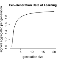
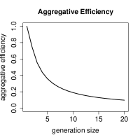
Figure 1: Left: A maximal generations network with a generation size of three. An arrow from $i$ to $j$ means $j$ observes $i$’s action. Middle: Number of signals aggregated per generation asymptotically in maximal generations networks, as a function of generation size. Right: Aggregative efficiency in maximal generations networks, as a function of generation size.

We also compare rational social-learning dynamics across different symmetric generations networks. We derive a simple formula for aggregative efficiency as a function of the network parameters. This expression shows the number of signals aggregated per generation increases in the number of neighbors for each agent and decreases in the level of confounding (i.e., the number of common neighbors for pairs of distinct agents in the same generation), thus quantifying the trade-offs in changing the network. For instance, increasing the density of the observation network may have two countervailing effects on learning: it can speed up the per-generation learning rate by adding more social observations, but also slow it down by lowering the informational content of each observation through extra confounding.

Our final result relates aggregative efficiency to welfare. If signals are sufficiently precise or the planner is sufficiently impatient, welfare will depend primarily on the learning outcomes of the first few agents. We relate aggregative efficiency to welfare outside of these cases: networks with higher aggregative efficiency lead to higher welfare when signals are not too precise and the social welfare function is sufficiently patient. We also give an example showing the arbitrarily large information loss in generations networks can have arbitrarily large welfare consequences.

2 Model

There are two equally likely states of the world, $\omega\in\{0,1\}$. An infinite sequence of agents indexed by $i\in\mathbf{\mathbb{N}_{+}}$ move in order, each acting once. (In some examples, we work with finite subsets $\{1,\ldots,n\}$ of this infinite sequence.) On her turn, agent $i$ observes a private signal $s_{i}\in\mathbb{R}$ and the actions of her neighbors, $N(i)\subseteq\{1,...i-1\}.$ Agent $i$ then chooses an action $a_{i}\in(0,1)$ to maximize the expectation of $u_{i}(a_{i},\omega)\coloneqq-(a_{i}-\omega)^{2}$ given all of her information. So her action is equal to her belief about the probability that $\omega=1$.

We consider a Gaussian information structure where private signals $(s_{i})$ are conditionally i.i.d. given the state. We have $s_{i}\sim\mathcal{N}(1,\sigma^{2})$ when $\omega=1$ and $s_{i}\sim\mathcal{N}(-1,\sigma^{2})$ when $\omega=0,$ where $\mathcal{N}(a,b^{2})$ is the Gaussian distribution with mean $a$ and variance $b^{2},$ and $0<1/\sigma^{2}<\infty$ is the private-signal precision.

Neighborhoods of different agents define a deterministic network $M$, where there is a directed link $j\rightarrow i$ if and only if $j\in N(i)$. We also view $M$ as the adjacency matrix, with $M_{i,j}=1$ if $j\in N(i)$ and $M_{i,j}=0$ otherwise. Since $N(i)\subseteq\{1,...,i-1\},$ $M$ is upper triangular. The network $M$ is common knowledge. The goal of this paper is to explore to what extent network structures can hinder efficient information aggregation.

With the network $M$ fixed, let $d_{i}:=|N(i)|$ denote the number of $i$’s neighbors. A strategy for agent $i$ is a function $A_{i}:(0,1)^{d_{i}}\times\mathbb{R}\to(0,1)$, where $A_{i}(a_{j(1)},...,a_{j(d_{i})},s_{i})$ specifies $i$’s play after observing actions $a_{j(1)},...,a_{j(d_{i})}$ from neighbors $N(i)=\{j(1),...,j(d_{i})\}$ and when her own private signal is $s_{i}$. There is a unique rational strategy profile $(A_{i}^{*})_{i\in\mathbb{N}_{+}}$ so that for all $i$ and for all observations of $i,$ $A_{i}^{*}$ maximizes Bayesian expected utility given the posterior belief about $\omega.$ Uniqueness of this profile follows from the sequential nature of the social-learning game and the existence of a unique optimal action at any belief. Agent 1 has no social observations, so there is a unique rational strategy $A_{1}^{*}(s_{1})$. This implies agent 2 also has a unique rational strategy $A_{2}^{*}$, as we have fixed the behavior of a rational agent 1. Proceeding in this way, there is a unique rational strategy profile $(A_{i}^{*})_{i\in\mathbb{N}_{+}}$.

3 Basic Results about Beliefs and Learning

In this section, we show that rational actions are log-linear and satisfy a signal-counting interpretation. We then use these properties to demonstrate informational confounds in several examples. The final subsection gives a condition for long-run learning and defines an asymptotic measure of how efficiently information is aggregated.

3.1 Optimal Actions Are Log-Linear

As is common in analyzing social-learning problems, we will find it convenient to work with the following log-transformations of variables: $\lambda_{i}\coloneqq\ln\left(\frac{\mathbb{P}[\omega=1|s_{i}]}{\mathbb{P}[\omega=0|s_{i}]}\right)$, $\ell_{i}\coloneqq\ln\left(\frac{a_{i}}{1-a_{i}}\right)$. We call $\lambda_{i}$ the log-signal of $i$ and $\ell_{i}$ the log-action of $i.$ These changes are bijective, so it is without loss to use the log versions. Write $\mathcal{L}_{i}^{*}(\ell_{j(1)},...,\ell_{j(d_{i})},\lambda_{i})$ for $i$’s rational log-strategy: the (unique) rational map from $i$’s neighbors’ log-actions and $i$’s log-signal to $i$’s log-action. In this section, we show that every $\mathcal{L}_{i}^{*}$ is a linear function of its arguments, with coefficients that only depend on the network $M$ and not on the precision of private signals.

The following result shows the optimal aggregation is linear in log-signals and log-actions (log-linear) and gives an explicit expression for the coefficients. All proofs are in the Appendix.

Proposition 1.

For each agent $i$ with $N(i)=\{j(1),...,j(d_{i})\},$ there exist constants $(\beta_{i,j(k)})_{k=1}^{d_{i}}$ so that $i$’s rational log-strategy is given by

$$\mathcal{L}_{i}^{*}(\ell_{j(1)},...,\ell_{j(d_{i})},\lambda_{i})=\lambda_{i}+\sum_{k=1}^{d_{i}}\beta_{i,j(k)}\ell_{j(k)}.$$

The vector of coefficients $\vec{\beta}_{i}$ is given by

$$\vec{\beta}_{i}=2\left(\mathbb{E}[(\ell_{j(1)},...,\ell_{j(d_{i})})\mid\omega=1]\times\textsc{\emph{Cov}}[\ell_{j(1)},...,\ell_{j(d_{i})}\mid\omega=1]^{-1}\right),$$

where $\textsc{\emph{Cov}}[\ell_{j(1)},...,\ell_{j(d_{i})}\mid\omega=1]^{-1}$ is the inverse of the conditional covariance matrix. These coefficients do not depend on the signal variance $\sigma^{2}.$

For general private-signal distributions, models of Bayesian updating in networks have tractability issues, as Golub and Sadler (2016) point out. The key lemma to proving Proposition 1 shows that given our Gaussian information structure, agent $i$’s observations have a jointly Gaussian distribution conditional on $\omega$. This permits us to study optimal inference in closed form. The interpretation of the inverse covariance matrix that appears in the coefficients $\vec{\beta}_{i}$ is that $i$ rationally discounts the actions of two neighbors $j(1)$ and $j(2)$ if their actions are conditionally correlated.

3.2 Measure of Accuracy

We would like to evaluate networks in terms of their social-learning accuracy so that we can compare the rates of Bayesian learning in different networks. Towards a measure of accuracy, imagine that agent $i$’s only information about $\omega$ consists of $n\in\mathbb{N}_{+}$ conditionally independent private signals. Then, the Bayesian $i$ would play the log-action equal to the sum of the $n$ log-signals, and it turns out (by Lemma A.1 in the Appendix) her behavior would follow the conditional distributions $\ell_{i}\sim\mathcal{N}\left(\pm n\cdot\frac{2}{\sigma^{2}},n\cdot\frac{4}{\sigma^{2}}\right)$, with the positive and negative means in states $\omega=1$ and $\omega=0$ respectively. We quantify learning accuracy using distributions of this form that allow for non-integer $n$, thus denominating accuracy in the units of private signals.

Definition 1.

Social learning aggregates $r\in\mathbb{R}_{+}$ signals by agent $i$ if the rational log-action $\ell_{i}$ has the conditional distributions $\mathcal{N}\left(\pm r\cdot\frac{2}{\sigma^{2}},r\cdot\frac{4}{\sigma^{2}}\right)$ in the two states. If this holds for some $r\in\mathbb{R}_{+}$, then we say $i$’s behavior has a signal-counting interpretation.

When agents use an arbitrary strategy profile, in general the conditional distributions of $\ell_{i}$ need not equal $\mathcal{N}\left(\pm r\cdot\frac{2}{\sigma^{2}},r\cdot\frac{4}{\sigma^{2}}\right)$ for any $r$, even when the strategy profile is log-linear (i.e., each agent’s log-action is a linear function of her log-signal and neighbors’ log-actions). Indeed, if this profile results in $i$ putting certain weights $(w_{i,j})_{j\leq i}$ on log-signals $(\lambda_{j})_{j\leq i},$ then $\ell_{i}$ has a signal-counting interpretation if and only if $\sum_{j=1}^{i}w_{i,j}=\sum_{j=1}^{i}w_{i,j}^{2}.$

But as the next result shows, the rational log-actions always admit a signal-counting interpretation in any network.

Proposition 2.

There exist $(r_{i})_{i\geq 1}$ so that social learning aggregates $r_{i}$ signals by agent $i.$ These $(r_{i})_{i\geq 1}$ depend on the network $M,$ but not on private-signal precision.

The signal-counting interpretation gives a way to compare agents’ accuracy and welfare across different networks or positions in a given network in a binary-state setting. Rather than comparing the full distributions of beliefs, we can compare the summary statistics $r_{i}$. A consequence is that agents’ beliefs, which a priori are multi-dimensional objects, are in fact ranked in the standard Blackwell ordering: a higher value of $r_{i}$ implies a weakly higher expected utility for any decision problem.

Such comparisons are straightforward in a different framework with a Gaussian state and Gaussian signals (e.g., Morris and Shin (2002) and, in the context of social learning, Dasaratha, Golub, and Hak (2020)). In these models, Bayesian agents’ beliefs are ranked by their precisions. The analogous number of signals aggregated is simply proportional to precision and so a signal-counting interpretation does not provide obvious additional insights. In the binary-state model used in most of the sequential social-learning literature (beginning with Banerjee (1992) and Bikhchandani et al. (1992)), however, the existence of such a ranking is not obvious and the signal-counting interpretation gives a distinct measure that considerably simplifies our analysis.

The signal-counting interpretation of behavior is closely identified with the rational learning rule. Indeed, a rational agent’s behavior always admits a signal-counting interpretation even when her predecessors use arbitrary non-rational log-linear strategies.

Corollary 1.

Fix arbitrary log-linear strategies for agents $i<I$. If agent $I$ best responds to these strategies, then $I$’s behavior has a signal-counting interpretation.

For a rational agent, Definition 1 gives a summary statistic for the accuracy of her beliefs and her utility—even if her observations are not generated by rational behavior. If an agent is not updating beliefs or choosing actions rationally, however, her utility need not be determined by such a summary statistic and can depend on a more complex action distribution.

3.3 Examples

We begin with several examples of social learning in networks with finitely many agents. These examples illustrate the basic obstruction to learning in our model, highlight the extent of possible information loss due to confounding, and provide intuition for our main results on generations networks.

Example 1 (The Shield and the Diamond).

Consider two network structures with four agents, as shown in Figure 2. In a shield network, agent $4$ observes agents $1,2,$ and $3$ while agents $2$ and $3$ observe agent $1$. In a diamond network, agent $4$ observes agents $2$ and $3$ while agents $2$ and $3$ observe agent $1$.

Figure 2: Left: The shield network with four agents. Right: The diamond network with four agents.

In a shield network, agent $4$ observes all predecessors and can compute the private signals of all agents. To see this, note that $\ell_{1}=\lambda_{1}$, $\ell_{2}=\lambda_{1}+\lambda_{2}$, and $\ell_{3}=\lambda_{1}+\lambda_{3}$. So

$$\ell_{4}=\lambda_{4}+\ell_{2}+\ell_{3}-\ell_{1}=\sum_{j=1}^{4}\lambda_{j}$$

is the optimal action given her private signal and those of her three predecessors, and $r_{4}=4$. As in Eyster and Rabin (2014), the optimal action involves anti-imitating, or placing a negative weight on, agent $1$’s action.

In a diamond network, however, agent $4$ observes the actions of agents $2$ and $3$ that combine their private signals with agent $1$’s signal, which agent $4$ does not observe. Agent $4$ faces an unavoidable tradeoff between overweighting agent $1$’s signal and underweighting agents $2$ and $3$’s signals. As in the shield network, we have $\ell_{1}=\lambda_{1}$, $\ell_{2}=\lambda_{1}+\lambda_{2}$, and $\ell_{3}=\lambda_{1}+\lambda_{3}$. Using Proposition 1, we can calculate that now

$$\ell_{4}=\lambda_{4}+\frac{2}{3}\ell_{2}+\frac{2}{3}\ell_{3}=\frac{4}{3}\lambda_{1}+\frac{2}{3}\lambda_{2}+\frac{2}{3}\lambda_{3}+\lambda_{4},$$

and therefore $r_{4}=\frac{11}{3}<4$. Even though agent $4$ is Bayesian and optimally adjusts for the confounding signal that she does not observe, some information is lost. This information loss is not too severe here, but the next example shows it can be much worse with more agents.

Example 2.

To see that confounding can lead to more severe information loss, we next generalize the diamond network to allow more agents. Consider a network with agents in three generations, shown in Figure 3. In the first generation, agents $1,2,\ldots,K_{1}$ have no neighbors. In the second generation, agents $K_{1}+1,K_{1}+2,\ldots,K_{1}+K_{2}$ observe all agents in the first generation. Finally, the third generation consists of a single agent who observes all agents in the second generation but does not observe the first generation. The purpose of this example is to study the beliefs of an agent with many neighbors who all observe a common confound.

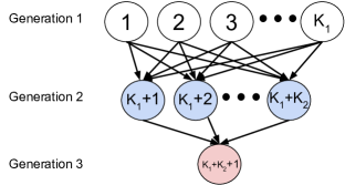
Figure 3: A three-generation network with $K_{1}$ agents in generation 1, $K_{2}$ agents in generation 2, and one agent in generation 3.

The agent in generation 3 rationally calculates the log-likelihood of state $\omega=1$ by taking a weighted sum of the log-actions of generation $2$ agents and her own signal, where the weights depend on $K_{1}$ and $K_{2}$. As in Example 1, the final agent faces an unavoidable tradeoff between overweighting generation $1$’s private signals and underweighting generation $2$’s private signals. Using Proposition 1, we can compute that the optimal action places weight $\frac{1+K_{1}}{1+K_{1}K_{2}}$ on each generation 2 action (see Appendix A.1 for details of the calculations in this example). When generation $2$ is large, this weight is close to $1/K_{2}$: it is optimal for the final agent to severely underweight the private signals of generation $2$.

We can also show that the actions of the agents in generation $2$ are distributed as if they see $1+K_{1}$ conditionally independent private signals, while the action of the final agent is distributed as if she sees $1+\frac{K_{2}+K_{1}K_{2}}{1+K_{1}K_{2}}\cdot(1+K_{1})$ such signals. The difference between the accuracy of generation $2$ and $3$’s actions is just

$$1+\frac{K_{2}+K_{1}K_{2}}{1+K_{1}K_{2}}\cdot(1+K_{1})-(1+K_{1})=1+\frac{(K_{2}-1)(K_{1}+1)}{K_{1}K_{2}+1}<3$$

private signals, for any values of $K_{1}$ and $K_{2}$. So there is always very little learning between generations $2$ and $3$, even when the size of generation $2$ is large and many private signals arrive in that generation. The idea is that confounding significantly limits how much information the final agent can extract from arbitrarily many neighbors’ actions.

We emphasize that the first generation can generate substantial confounding even when it is small. For example, if there is a single agent in the first generation ($K_{1}=1$), then the action of the agent in generation $3$ will be less accurate than that of someone who saw just five independent private signals. But if generation $1$ were empty, then the action of the generation 3 agent would be equivalent to $K_{2}+1$ private signals. So even a small confound can prevent almost all information aggregation. Also, a simple calculation shows that the difference between the accuracy of generation 2 and generation 3 strictly decreases in $K_{1}$ and strictly increases in $K_{2},$ provided $K_{2}\geq 2.$ That is, the incremental amount of learning in the final generation decreases with confounding (a larger $K_{1})$ but increases with the number of observations (a larger $K_{2}).$ We will later see that the same comparative statics hold for a class of infinite networks where agents move in generations.

3.4 Long-Run Learning and Aggregative Efficiency

We now return to studying infinite networks. We begin with a benchmark result providing necessary and sufficient conditions for long-run learning. These conditions turn out to be similar to those in the existing literature, which shows our model is comparable to the standard models on this dimension. A key contribution of our model is ranking networks where agents learn in the long run based on the rate of this learning, and this section concludes by defining a measure that will provide such a ranking for a class of generation networks.

We say society learns completely in the long run if $(a_{i})$ converges to $\omega$ in probability. For a given network $M,$ write $\mathcal{PL}(i)\in\mathbb{N}$ to refer to the length of the longest path in $M$ originating from $i$ (this length is 0 if $N(i)=\varnothing$).

Proposition 3.

The following are equivalent: (1) $\lim\limits_{{\it i\to\infty}}\mathcal{PL}(i)=\infty$; (2) $\lim\limits_{{\it i\to\infty}}\left[\max_{j\in N(i)}j\right]=\infty$; (3) $\lim_{i\to\infty}r_{i}=\infty$; (4) society learns completely in the long run.

Condition (2) is the analog of Acemoglu, Dahleh, Lobel, and Ozdaglar (2011)’s expanding observations property for a deterministic network. It says if we consider the most recent neighbor observed by each agent, then this sequence of most recent neighbors tends to infinity. It is straightforward to see the expanding observations condition is necessary for long-run learning, and Acemoglu et al. (2011) show it is also sufficient in a random-networks model with unboundedly informative signals and binary actions. With continuous actions, Proposition 3 states the same result. The intuition is that each agent learns at least as well as if she optimally combined her most accurate social observation with her private signal.

The key takeaway message from Proposition 3 is that whether society learns in the long run is not a useful criterion for comparing different networks in this setting, as the conditions (1) and (2) that guarantee long-run learning are quite mild. It is of course possible that agents learn completely but do so very slowly. We now define a measure of the efficiency of learning, which can evaluate learning outcomes when this occurs:

Definition 2.

If $\lim_{i\to\infty}(r_{i}/i)$ exists, it is called the aggregative efficiency of the network.

Aggregative efficiency measures the fraction of signals in the entire society that individuals manage to aggregate under social learning. Networks with higher levels of aggregative efficiency induce faster social learning in the long run. The limit defining aggregative efficiency need not exist in all networks, but does exist in all of the examples we focus on.

The next section will compare how quickly $(r_{i})_{i\geq 1}$ grows across a class of generations networks and the aggregative efficiency of these networks. Comparisons of aggregative efficiency also translate into welfare comparisons, as Section 5 will show.

4 Generations Networks

This section shows that informational confounding can lead to arbitrarily large information losses and derives a closed-form expression for how confounding influences learning in a class of networks. We study generations networks and find that they can lead to very inefficient learning due to confounding. We also compare aggregative efficiency across these networks.

Figure 4: A generations network with $K=3$ agents per generation and the observation sets $\Psi_{1}=\{1,2\},$ $\Psi_{2}=\{2,3\},$ and $\Psi_{3}=\{1,3\}$.

Agents are sequentially arranged into generations of size $K$, with agents within each generation placed into positions 1 through $K.$ Agents in the first generation (i.e., $i=1,...,K$) have no neighbors. A collection of observation sets $\Psi_{k}\subseteq\{1,...,K\}$ for $k=1,...,K$ define the network $M$ for agents in later generations. The agent in position $k$ in generation $t\geq 2$ observes agents in positions $\Psi_{k}$ from generation $t-1$ (and no agents from any other generation). That is, for $i=(t-1)K+k$ where $t\geq 2$ and $1\leq k\leq K,$ network $M$ has $N(i)=\{(t-2)K+\psi:\psi\in\Psi_{k}\}.$ Figure 4 shows an example with $K=3$.

We focus on observation sets $(\Psi_{k})_{k}$ satisfying a symmetry condition:

Definition 3.

The observation sets are symmetric if all agents observe $d\geq 1$ neighbors and all pairs of agents in the same generation share $c$ common neighbors, i.e. $|\Psi_{k}|=d$ for every $1\leq k\leq K$ and $|\Psi_{k_{1}}\cap\Psi_{k_{2}}|=c$ for distinct positions $1\leq k_{1}<k_{2}\leq K$.

A generations network defined by symmetric observation sets is called a symmetric network. To give a class of examples of symmetric networks, fix any non-empty subset $E\subseteq\{1,...,K\},$ and let $(\Psi_{k})_{k}$ be such that for all $1\leq k\leq K,$ $\Psi_{k}=E.$ Here we have $d=c=|E|.$ To interpret, the set $E$ represents the prominent positions in the society, and agents only observe predecessors in these prominent positions from the past generation. We call the special case of $E=\{1,...,K\}$ the maximal generations network, where agents in generation $t$ for $t\geq 2$ have all agents in generation $t-1$ as their neighbors. For another class of examples, suppose $K\geq 2$ and each agent observes a different subset of $K-1$ predecessors from the previous generation. Specifically, $\Psi_{k}=\{1,...,K\}\backslash\{k-1\}$ for $2\leq k\leq K,$ and $\Psi_{1}=\{1,...,K-1\}.$ This network is symmetric with $d=K-1$ and $c=K-2.$ (The network in Figure 4 has this structure, with $d=2$ and $c=1$.) There remains a large variety of other symmetric networks that are not covered by these two classes of examples: one enumeration shows there are at least 103 pairs of feasible $(d,c)$ parameters in the range of $3\leq d\leq 41$ and $1\leq c\leq d-2$ that correspond to at least one symmetric network, typically with multiple non-isomorphic networks for each feasible parameter pair (Mathon and Rosa, 1985).

4.1 Aggregative Efficiency in Symmetric Generations Networks

We provide an exact expression for the aggregative efficiency in symmetric generations networks to quantify the information loss due to confounding.

Theorem 1.

Given any symmetric observation sets $(\Psi_{k})_{k}$ where every agent observes $d$ neighbors and every pair of agents in the same generation share $c$ common neighbors, aggregative efficiency is

$$\lim_{i\to\infty}(r_{i}/i)=\left(1+\frac{d^{2}-d}{d^{2}-d+c}\right)\frac{1}{K}$$

The number of signals aggregated per generation asymptotically $(\lim_{i\to\infty}r_{i+K}-r_{i})$ is less than $2$. For $c\geq 1,$ this number is strictly increasing in $d$ and strictly decreasing in $c$.

Theorem 1 calculates the aggregative efficiency in any symmetric generations network in terms of the parameters $d$ and $c$. The expression on the right-hand side normalizes by the size of the generation $K,$ so the term in the parentheses provides a uniform learning-rate upper bound of two signals per generation across all symmetric networks (as $\frac{d^{2}-d}{d^{2}-d+c}\leq 1$).

The interpretation of the comparative statics result in $d$ and $c$ is that more observations speed up the rate of learning per generation but more confounding slows it down, all else equal. This result lets us compare learning dynamics across different symmetric networks characterized by different $(d,c)$ parameter pairs. Changing from one network to another, we can change both $d$ and $c$ (along with the generation size $K$). Theorem 1 decomposes the repercussions of such changes on the per-generation learning rate (i.e., after normalizing by $1/K)$ into their effects on the two primitive network parameters that have monotonic influences on said rate.

The main content of the theorem is the uniform bound on the learning rate, which implies learning is very inefficient in large symmetric generations networks. The proof of Proposition 3 provides a lower bound of one signal aggregated per generation, since agents could always optimally combine their private signal with one observed action. Theorem 1 shows this lower bound is not too far from the actual learning rate, which is fewer than two signals per generation.

For maximal generations networks (i.e., agents observe all predecessors from the previous generation), the basic intuition for this bound is similar to Example 2, which tells us that when any number of agents observe one or more common signals in addition to their private signals, a successor who observes all of these agents cannot improve on their accuracy by more than three signals worth of information. The successor must balance overweighting the common confound and underweighting her neighbors’ private signals, and the optimal weights severely underweight recent signals.

Extending this intuition beyond maximal generations networks is more subtle, because different agents in a generation may observe different predecessors whose actions may be less correlated. This can alleviate the informational confounding in early generations, but we show the benefits are limited: even if agents in the same generation have almost disjoint observation sets, actions become highly correlated in later generations. To prove this, we use a mixing argument to show that the actions of two agents in the same generation are influenced in very similar ways by the signal realizations of their common ancestors from many generations ago. An implication is that recent signals are severely underweighted, as in the maximal generations case: the total weight an agent places on private signals from the previous generation converges to one, while in the absence of network-based confounds the agent would place a weight of one on each signal.

By specializing Theorem 1 to the case of $d=c=K,$ we can calculate the aggregative efficiency of maximal generations networks.

Corollary 2.

Consider a maximal generations network with $K\geq 1$. We have $\lim_{i\to\infty}(r_{i}/i)=\frac{(2K-1)}{K^{2}}$, so aggregative efficiency is lower with larger $K.$

Indeed, if $K=1,$ then every agent perfectly incorporates all past private signals and the speed of social learning is the highest possible. Not only does this result about the aggregative efficiency imply that asymptotically fewer signals are aggregated by the same agent in networks with larger $K$, but the same comparative statics also hold numerically for all agents $i\geq 16$ when comparing among $K\in\{2,3,4,5\}$, as shown in Figure 5. Finally, note that the number of signals aggregated per generation in the long run increases in $K,$ but (by Theorem 1) this number is always bounded by two.

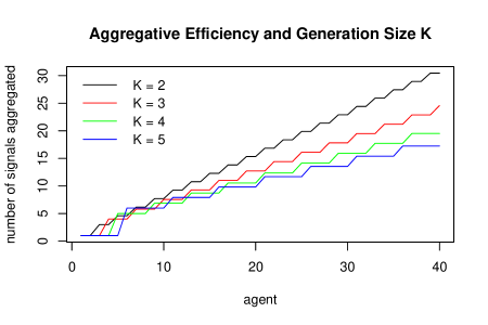
Figure 5: Number of signals aggregated by social learning in maximal generations networks with different generation sizes, $K\in\{2,3,4,5\}.$

In maximal generations networks, if an agent could additionally observe the private signal of even one agent from the previous generation, then she could calculate the common confounding information and fully compensate for this confound. In networks with large $K$, showing each agent just one extra signal (of someone from the previous generation) increases aggregative efficiency from nearly 0 to 1.

We next discuss the role of the symmetric generations structure in the bound of two additional signals per generation. We have implicitly imposed three restrictions on the network, beyond the basic generations structure: the observation structures are the same across generations, all generations are the same size, and observations are symmetric within generations. We assume the same observation structure across generations primarily for simplicity of exposition, and could bound aggregative efficiency with the same techniques while allowing different symmetric observation structures in different generations. The key step in extending the proof is the Markov chain mixing result, which must be replaced by a mixing result for non-homogeneous Markov chains (for examples of such results, see Blackwell (1945) and Tahbaz-Salehi and Jadbabaie (2006)). We could also allow different sized generations and obtain bounds on aggregative efficiency. For example, the logic of Example 2 would extend to maximal generation networks with generations of varying sizes.

The assumption of symmetry within generations is more substantive, and our bound of two signals of additional information per generation does not always apply to non-symmetric generations networks. For example, suppose $\Psi_{k}=\{k\}$ for some position $k$. The accuracy of agents in this position will only increase by one additional signal per generation, but these agents can aggregate independent information that can be valuable to agents in other positions. An unresolved question is whether asymmetric observation structures could let all agents aggregate more than two signals per generation.

Finally, we show that aggregative efficiency in symmetric networks only depends on the generation size. An insight that extends from maximal generations networks to any symmetric networks is that aggregative efficiency is worse with larger generations. Compare the symmetric network from Figure 4 with $d=2,c=1,K=3$ with the maximal generations network with $K=3$. Theorem 1 implies they have the same aggregative efficiency. The extra social observations in the second network exactly cancel out the reduced informational content of each observation, due to the more severe informational confounds. It turns out that more generally, any symmetric network with parameters $(d,c,K)$ where $d\geq 2$, $c<d$ has the same aggregative efficiency as the maximal generations network with the same generation size $K$. Therefore, the idea of worse efficiency with larger generations depicted in Figure 5 for maximal generations networks also holds in the broader class of symmetric networks.

Corollary 3.

In any symmetric network with $d\geq 2$, aggregative efficiency is $\lim_{i\to\infty}(r_{i}/i)=(2-(1/K))\cdot\frac{1}{K}.$

This corollary follows from the fact that the symmetry condition imposes some combinatorial constraints on the feasible $(d,c,K)$ parameter triplets. It turns out these constraints allow us to simplify the expression in Theorem 1 when we know the generation size. While Corollary 3 gives a simple expression of aggregative efficiency that just depends on $K$, Theorem 1 lets us compare networks that differ in $d$ and $c$ (and possibly also $K$) more transparently.

4.2 Finite-Population Learning

Our framework not only allows us to study the asymptotic rate of learning, but also lets us derive finite-population bounds that apply from early generations. Theorem 1 tells us social learning aggregates fewer than two signals per generation asymptotically. There is also a short-run version of this result in the maximal generations network: starting with generation 3, fewer than three signals are aggregated per generation for any $K$.

Proposition 4.

In any maximal generations network, for any agents $i,i^{{}^{\prime}}$ in generation $t$ and $t-1$ with $t\geq 3,$ $r_{i}-r_{i^{{}^{\prime}}}\leq 3$.

We find an even starker bound on $r_{i}$ if we consider a modified version of the maximal generations network: there is a zeroth generation with only one agent, and all subsequent generations contain $K$ agents each. Agents in generation $t\geq 1$ observe all predecessors from generation $t-1.$

Proposition 5.

In this modified maximal generations network, $r_{i}\leq 3t-1$ for every $i$ in every generation $t\geq 1$.

Similar to Example 2, the single agent before the first generation causes significant information confounding. With this additional agent, there is a uniform bound on every generation’s accuracy across all generation sizes $K$.

5 Aggregative Efficiency and Welfare

In this section, we relate aggregative efficiency comparisons to welfare comparisons. When signals are precise enough for agents to learn well, welfare will depend largely on learning outcomes of finite networks (such as the examples in Section 3.3) rather than asymptotic quantities. Higher aggregative efficiency implies higher welfare, however, when signals are sufficiently imprecise.

Let $v_{i}^{M}:=\mathbb{E}[u_{i}(a_{i}^{*},\omega)]$ denote the expected welfare of agent $i$ in network $M$, and recall that $-0.25<v_{i}^{M}<0$ for every $i$ in any network and with any private signal precision $0<1/\sigma^{2}<\infty.$ It turns out that whenever the aggregative efficiency of a network $M$ is strictly positive, $v_{i}^{M}\to 0$ and this convergence happens at an exponential rate. This implies the undiscounted sum of utilities of all agents, $\sum_{i}v_{i}^{M}$, is convergent.

We show that if two networks are ranked by aggregative efficiency, then the undiscounted sums of all agents’ utilities on these networks follow the same ranking whenever private signals are sufficiently imprecise. The same result also applies to the discounted sums of utilities, provided the discounting does not weigh the welfare of the earliest agents too heavily.

Proposition 6.

Suppose networks $M$ and $M^{\prime}$ have aggregative efficiencies $AE_{M}>AE_{M^{\prime}}>0.$ Then there exists some $\underline{\sigma}^{2}>0$ such that for any signal variance $\sigma^{2}\geq\underline{\sigma}^{2}$, we have $\sum_{i}\delta^{i-1}v_{i}^{M}>\sum_{i}\delta^{i-1}v_{i}^{M^{\prime}}$ for $\delta$ sufficiently close to or equal to $1$.

This result provides a foundation for the aggregative efficiency measure in terms of a conventional social welfare function: the (un)discounted sum of utilities. The result applies to arbitrary networks, and does require the generations structure from Section 4.

The arbitrarily large information loss we have highlighted in Section 4 can have large welfare consequences. To illustrate this, we give an example comparing complete networks to maximal generations networks with large generations.

Example 3.

Let $M$ be the maximal generations network with generation size $K$. We will let $K$ grow large and set signal variance $\sigma^{2}=\sigma_{0}^{2}/K$ for a constant $\sigma_{0}^{2}>0$. That is, we increase the generation size but fix the total informativeness of a single generation’s private signals. Let $M^{\prime}$ be the complete network (or any other network with $r_{i}=i$ for all $i$). Then

$$\lim_{K\rightarrow\infty}\frac{\sum_{i}v_{i}^{M}}{\sum_{i}v_{i}^{M^{\prime}}}=\infty.$$

(We provide an argument in Appendix A.) Since utilities are negative for all agents, the limit implies that the total disutility in the maximal generations network is unboundedly larger than when agents can extract all previous private signals.

6 Related Literature

We study rational social learning in a sequential model (as first introduced by Banerjee (1992) and Bikhchandani, Hirshleifer, and Welch (1992)) where agents only observe some predecessors. Our work contributes to the social learning literature by quantifying how parameters of the network structure affect the efficiency of social learning. This leads us to the new conclusion that a small amount of network confounding can generate arbitrarily inefficient social learning, even when agents perfectly observe their neighbors’ beliefs.

Our paper continues a literature on sequential learning when private signals can generate unboundedly strong beliefs. Smith and Sørensen (2000) show that there is complete long-run learning on the complete network with such signals, and Acemoglu, Dahleh, Lobel, and Ozdaglar (2011) and Lobel and Sadler (2015) extend this result to all networks satisfying weak sufficient conditions (see Proposition 3). Rosenberg and Vieille (2019) consider several networks without the type of confounding we study and reach a similar conclusion that “the nature of the feedback on previous choices matters little” (under a different criterion for good learning). Our results on information confounds show that network structure can matter substantially, however, for short-run accuracy and rates of learning. The most closely related network-based obstructions to learning appear in Eyster and Rabin (2014), who mention the possibility of such confounds but restrict their analysis to networks where rational agents can fully correct for correlations in observations via anti-imitation. They note that relaxing this restriction to allow confounds would lead to “distributional complications”; our framework and results resolve these complications and study the implications of the confounds. We also compare learning rates across networks; a related precedent is Lobel, Acemoglu, Dahleh, and Ozdaglar (2009), who examine two particular networks, both involving each agent seeing exactly one neighbor. Theorem 1 and Corollary 2 allow us to rank a class of generations networks which vary along several dimensions, including the number of neighbors agents have.

Complete long-run learning fails in sequential models with boundedly informative signals (Smith and Sørensen, 2000), so these models provide an alternative setting for asking how network structure affects learning. In this setting, several papers show that incomplete networks where some agents do not observe others lead to better long-run outcomes than the complete network (Sgroi, 2002; Acemoglu, Dahleh, Lobel, and Ozdaglar, 2011; Arieli and Mueller-Frank, 2019). These papers compare a specific class of incomplete networks with the complete network, but do not allow one to compare different incomplete networks (except through numerical simulations). We show a framework with Gaussian signals has useful properties such as log-linear actions and the signal-counting measure of accuracy and do not consider bounded signals, but we think further analytic results on the role of network structure in settings with bounded signals could be an interesting direction for future work.

Board and Meyer-ter Vehn (2021) study how network structure affects learning from peers in the context of product diffusion. Their environment is different from ours: whereas our paper focuses on the canonical sequential social-learning environment, Board and Meyer-ter Vehn (2021) look at a world where perfectly informative private signals about product quality diffuse through observations of others’ adoption choices. Due to this difference in setting, networks matter through distinct channels. We highlight a confounding mechanism where multiple neighbors of $i$ learn from a common source unavailable to $i$, and show this can make $i$’s learning arbitrarily inefficient. Such confounding does not appear (or has vanishing probability) in Board and Meyer-ter Vehn (2021). On the other hand, the agents in Board and Meyer-ter Vehn (2021) draw inferences over time about product quality from the absence of adoptions. Network structure affects these inferences because the absence of adoption creates more pessimism on networks where neighbors adopt faster when the product is good (e.g., sparse random networks).

Another strand of the literature, which does not involve network structure, examines other obstructions to efficient social learning. These papers study issues orthogonal to the social network structure and assume agents observe all predecessors. Harel, Mossel, Strack, and Tamuz (2021) study a social-learning environment with coarse communication and find, as in our generations network, that agents learn at the same rate as they would if they perfectly observed an arbitrarily small fraction of private signals. The mechanism behind their result (“rational groupthink”) is not related to an observation network preventing some agents from seeing others’ social information, but rather relies on agents’ finite action spaces obscuring all information about their private signals for many periods. Another group of papers point out that if signals about the state come from myopic agents’ information-acquisition choices, then individuals can make socially inefficient choices and slow down learning (Burguet and Vives, 2000; Mueller-Frank and Pai, 2016; Ali, 2018a; Lomys, 2020; Liang and Mu, 2020). We assume rich action spaces and exogenous signals to abstract from these obstructions and focus on the role of the network.

7 Conclusion

This paper presents a tractable model of sequential social learning that lets us compare social-learning dynamics across different observation networks. In our environment, rational actions are a log-linear function of observations and admit a signal-counting interpretation. Thus, we can measure the efficiency of learning in terms of the fraction of available signals incorporated into beliefs asymptotically (“aggregative efficiency”) and make precise comparisons about the rate of learning and welfare across different networks.

The network confounds learning when an agent does not see an early predecessor whose action influenced several of the agent’s neighbors. We show that confounding is a powerful obstacle to social learning: even little confounding can cause almost total information loss. For a class of symmetric networks where agents move in generations, we derive an analytic expression for aggregative efficiency. For any network in this class, social learning aggregates no more than two signals per generation in the long run, even for arbitrarily large generations. We also compute comparative statics of learning with respect to network parameters, finding that additional observations speed up learning but extra confounding slows it down.

We have focused on how the network structure affects social learning and abstracted away from many other sources of learning-rate inefficiency. These other sources may realistically co-exist with the informational-confounding issues discussed here and complicate the analysis. For instance, even though the complete network allows agents to exactly infer every predecessor’s private signal, it could lead to worse informational free-riding incentives in settings where agents must pay for the precision of their private signals (compared to networks where agents have fewer observations). Studying the trade-offs and/or interactions between network-based information confounds and other obstructions to fast learning could lead to fruitful future work.

Appendix

Appendix A Proofs

A.1 Details on Example 2

We show that for the network in Figure 3, agent $K_{1}+K_{2}+1$’s rational log-strategy puts weight $\frac{1+K_{1}}{1+K_{1}K_{2}}$ on each neighbor’s log-action, and hence $r_{K_{1}+K_{2}+1}=1+\frac{K_{2}+K_{1}K_{2}}{1+K_{1}K_{2}}\cdot(1+K_{1}).$

For $1\leq j\leq K_{2},$ we have $\ell_{K_{1}+j}=\sum_{i=1}^{K_{1}}\lambda_{i}+\lambda_{K_{1}+j}$. So, $\mathbb{E}[\ell_{K_{1}+j}\mid\omega=1]=(K_{1}+1)\cdot\frac{2}{\sigma^{2}}$, $\text{Var}[\ell_{K_{1}+j}\mid\omega=1]=\frac{4}{\sigma^{2}}(K_{1}+1)$, while $\text{Cov}[\ell_{K_{1}+j},\ell_{K_{1}+j^{\prime}}\mid\omega=1]=\frac{4}{\sigma^{2}}K_{1}$ for $1\leq j<j^{\prime}\leq K_{2}$. By Proposition 1, the vector of weights that the final agent’s rational log-strategy puts on neighbors’ log actions is given by

$$2\cdot\frac{2}{\sigma^{2}}\cdot\left[\begin{array}[]{ccc}K_{1}+1&K_{1}+1&\cdots\end{array}\right]\cdot\frac{\sigma^{2}}{4}\cdot\begin{array}[]{c}\underset{K_{2}\text{ by }K_{2}}{\underbrace{\left[\begin{array}[]{cccc}K_{1}+1&K_{1}&\cdots&K_{1}\\ K_{1}&K_{1}+1&\cdots&K_{1}\\ \vdots&\vdots&\ddots&\vdots\\ K_{1}&K_{1}&\cdots&K_{1}+1\end{array}\right]}}\end{array}^{-1}.$$

The matrix inverse is equal to

$$\frac{1}{K_{1}K_{2}+1}\underset{K_{2}\text{ by }K_{2}}{\underbrace{\left[\begin{array}[]{cccc}(K_{2}-1)K_{1}+1&-K_{1}&\cdots&-K_{1}\\ -K_{1}&(K_{2}-1)K_{1}+1&\cdots&-K_{1}\\ \vdots&\vdots&\ddots&\vdots\\ -K_{1}&-K_{1}&\cdots&(K_{2}-1)K_{1}+1\end{array}\right]}}.$$

Therefore, weight on each neighbor is $\frac{1+K_{1}}{1+K_{1}K_{2}}.$ Also, since $\mathbb{E}[\ell_{K_{1}+j}\mid\omega=1]=(K_{1}+1)\cdot\frac{2}{\sigma^{2}}$ for each neighbor $K_{1}+j$ and there are $K_{2}$ neighbors, we get $\mathbb{E}[\ell_{K_{1}+K_{2}+1}\mid\omega=1]=[1+\frac{K_{2}+K_{1}K_{2}}{1+K_{1}K_{2}}\cdot(1+K_{1})]\cdot\frac{2}{\sigma^{2}}$. By the signal counting interpretation, $r_{K_{1}+K_{2}+1}=1+\frac{K_{2}+K_{1}K_{2}}{1+K_{1}K_{2}}\cdot(1+K_{1}).$

A.2 Proof of Proposition 1

We first prove a lemma about the conditional distributions of the log-signals.

Lemma A.1.

For each $i,$ the log-signal $\lambda_{i}$ has a Gaussian distribution conditional on $\omega$, with $\mathbb{E}[\lambda_{i}\mid\omega=0]=-2/\sigma^{2},$ $\mathbb{E}[\lambda_{i}\mid\omega=1]=2/\sigma^{2},$ and $\textsc{\emph{Var}}[\lambda_{i}\mid\omega=0]=\textsc{\emph{Var}}[\lambda_{i}\mid\omega=1]=4/\sigma^{2}.$

Proof.

We show that $\lambda_{i}=\frac{2}{\sigma^{2}}s_{i}.$ This is because

$$\lambda_{i} =\ln\left(\frac{\mathbb{P}[\omega=1|s_{i}]}{\mathbb{P}[\omega=0|s_{i}]}\right)=\ln\left(\frac{\mathbb{P}[s_{i}|\omega=1]}{\mathbb{P}[s_{i}|\omega=0]}\right)=\ln\left(\frac{\exp\left(\frac{-(s_{i}-1)^{2}}{2\sigma^{2}}\right)}{\exp\left(\frac{-(s_{i}+1)^{2}}{2\sigma^{2}}\right)}\right)$$

$$=\frac{-(s_{i}^{2}-2s_{i}+1)+(s_{i}^{2}+2s_{i}+1)}{2\sigma^{2}}=\frac{2}{\sigma^{2}}s_{i}.$$

The result then follows from scaling the conditional distributions of $s_{i},$ $(s_{i}\mid\omega=1)\sim\mathcal{N}(1,\sigma^{2})$ and $(s_{i}\mid\omega=0)\sim\mathcal{N}(-1,\sigma^{2})$. ∎

Now we prove Proposition 1.

Proof.

Agent 1 does not observe any predecessors, so clearly $\mathcal{L}_{1}^{*}(\lambda_{1})=\lambda_{1}.$ Suppose by way of induction that the rational strategies of all agents $j\leq I-1$ are linear. Then each $\ell_{j}$ for $j\leq I-1$ is a linear combination of $(\lambda_{h})_{h=1}^{I},$ which by Lemma A.1 are conditionally Gaussian with conditional means $\pm 2/\sigma^{2}$ in states $\omega=1$ and $\omega=0$ and conditional variance $4/\sigma^{2}$ in each state. This implies $(\ell_{j(1)},...,\ell_{j(n_{I})})$ have a conditional joint Gaussian distribution with $(\ell_{j(1)},...,\ell_{j(n_{I})})\sim\mathcal{N}(\vec{\mu},\Sigma)$ conditional on $\omega=1$, and $(\ell_{j(1)},...,\ell_{j(n_{I})})\sim\mathcal{N}(-\vec{\mu},\Sigma)$ conditional on $\omega=0$, where $\vec{\mu}=\mathbb{E}[(\ell_{j(1)},...,\ell_{j(d_{i})})^{\prime}\mid\omega=1]$ and $\Sigma=\textsc{Cov}[\ell_{j(1)},...,\ell_{j(d_{i})}\mid\omega=1]$.

From the the multivariate Gaussian density, (writing $(\ell_{j(1)},...,\ell_{j(n_{I})})^{\prime}=\vec{a})$,

$$\ln\left(\frac{\mathbb{P}[\ell_{j(1)},...,\ell_{j(n_{I})}\mid\omega=1]}{\mathbb{P}[\ell_{j(1)},...,\ell_{j(n_{I})}\mid\omega=0]}\right) =\ln\left(\frac{\exp(-\frac{1}{2}(\vec{a}-\vec{\mu})^{\prime}\Sigma^{-1}(\vec{a}-\vec{\mu}))}{\exp(-\frac{1}{2}(\vec{a}+\vec{\mu})^{\prime}\Sigma^{-1}(\vec{a}+\vec{\mu}))}\right)$$

$$=\vec{a}^{\prime}\Sigma^{-1}\vec{\mu}+\vec{\mu}^{\prime}\Sigma^{-1}\vec{a}$$

which is $2\left(\vec{\mu}^{\prime}\Sigma^{-1}\right)\cdot(\ell_{j(1)},...,\ell_{j(n_{I})})^{\prime}$ because $\Sigma$ is symmetric. This then shows agent $I$’s rational strategy must also be linear, completing the inductive step. This argument also gives the explicit form of $\vec{\beta}_{I,\cdot}$.

For the final statement, we prove another lemma. The argument so far implies that we may find weights $(w_{i,j})_{j\leq i}$ so that the realizations of rational log-actions are related to the realizations of log-signals by $\ell_{i}=\sum_{j=1}^{i}w_{i,j}\lambda_{j}$. Let $W$ be the matrix containing all such weights.

Lemma A.2.

Let $\hat{W}$ be the submatrix of $W$ with rows $N(i)$ and columns $\{1,...,i-1\}.$Then $\vec{\beta}_{i}=\vec{\boldsymbol{1}}_{(i-1)}^{\prime}\times\hat{W}^{\prime}(\hat{W}\hat{W}^{\prime})^{-1}$ and the $i$-th row of $W$ is $W_{i}=\left((\vec{\beta}_{i,\cdot}^{\prime}\times\hat{W}),1,0,0,...\right)$.

Proof.

Suppose $N(i)=\{j(1),...,j(d_{i})\}$ with $j(1)<...<j(d_{i}).$ By Lemma A.1 and construction of $\hat{W}$, we have $\mathbb{E}[\ell_{j(k)}\mid\omega=1]=\frac{2}{\sigma^{2}}\sum_{h=1}^{i-1}\hat{W}_{k,h}$. So, $\mathbb{E}[(\ell_{j(1)},...,\ell_{j(d_{i})})\mid\omega=1]=\frac{2}{\sigma^{2}}(\hat{W}\cdot\boldsymbol{1}_{(i-1)})^{\prime}=\frac{2}{\sigma^{2}}\boldsymbol{1}_{(i-1)}^{\prime}\hat{W}{}^{\prime}.$ Also, again by Lemma A.1 and construction of $\hat{W}$, we can calculate that for $1\leq k_{1}\leq k_{2}\leq d_{i},$ $\textsc{Cov}[\ell_{j(k_{1})},\ell_{j(k_{2})}\mid\omega=1]=\frac{4}{\sigma^{2}}\sum_{h=1}^{i-1}(\hat{W}_{k_{1},h}\hat{W}_{k_{2},h}),$ meaning $\textsc{Cov}[\ell_{j(1)},...,\ell_{j(d_{i})}\mid\omega=1]=\frac{4}{\sigma^{2}}\hat{W}\hat{W}^{\prime}.$ It then follows from what we have shown above that $\vec{\beta}_{i,\cdot}=2\cdot\frac{2}{\sigma^{2}}\boldsymbol{1}_{(i-1)}^{\prime}\hat{W}{}^{\prime}\times\left[\frac{4}{\sigma^{2}}\hat{W}\hat{W}^{\prime}\right]^{-1}=\vec{\boldsymbol{1}}_{(i-1)}^{\prime}\times\hat{W}^{\prime}(\hat{W}\hat{W}^{\prime})^{-1}.$

Since $i$ puts weight 1 on $\lambda_{i}$ and weights $\vec{\beta}_{i,\cdot}$ on $(\ell_{j(1)},...,\ell_{j(d_{i})})^{\prime}=\hat{W}\times(\lambda_{1},...,\lambda_{i-1})^{\prime},$ this shows the first $i-1$ elements in the row $W_{i}$ must be $\vec{\beta}_{i,\cdot}^{\prime}\cdot\hat{W}$ while the $i$-th element is 1. ∎

To prove the final statement of Proposition 1, first observe that $W_{1}=(1,0,0,...)$ does not depend on $\sigma^{2}.$ The same applies to $\vec{\beta}_{1,\cdot}$. By way of induction, suppose rows $W_{i}$ and vectors $\vec{\beta}_{i,\cdot}$ do not depend on $\sigma^{2}$ for any $i\leq I$. If $\hat{W}$ is the submatrix of $W$ with rows $N(I+1)$, then since $N(I+1)\subseteq\{1,...,I\},$ by the inductive hypothesis $\hat{W}$ must be independent of $\sigma^{2}$. Thus the same independence also applies to $\vec{\beta}_{I+1,\cdot}$ since this vector only depends on $\hat{W}$ by the result just derived. In turn, since $W_{I+1}$ is only a function of $\vec{\beta}_{I+1,\cdot}^{\prime}$ and $\hat{W}$, and these terms are independent of $\sigma^{2}$ as argued before, same goes for $W_{I+1},$ completing the inductive step. ∎

A.3 Proof of Proposition 2

Proof.

It suffices to show that $\mathbb{E}[\ell_{i}\mid\omega=1]=\frac{1}{2}\textsc{Var}\left[\ell_{i}\mid\omega=1\right]$. By Proposition 1, $\ell_{i}=\lambda_{i}+\sum_{k=1}^{d_{i}}\beta_{i,j(k)}\ell_{j(k)}$. From Lemma A.1, we have $\mathbb{E}[\lambda_{i}\mid\omega=1]=\frac{1}{2}\textsc{Var}\left[\lambda_{i}\mid\omega=1\right]$. Furthermore, $\lambda_{i}$ is independent from $\sum_{k=1}^{d_{i}}\beta_{i,j(k)}\ell_{j(k)},$ as the latter term only depends on $\lambda_{1},...,\lambda_{i-1}.$ So we need only show $\mathbb{E}[\sum_{k=1}^{d_{i}}\beta_{i,j(k)}\ell_{j(k)}\mid\omega=1]=\frac{1}{2}\textsc{Var}\left[\sum_{k=1}^{d_{i}}\beta_{i,j(k)}\ell_{j(k)}\mid\omega=1\right]$

Let $\vec{\mu}=\mathbb{E}[(\ell_{j(1)},...,\ell_{j(d_{i})})^{\prime}\mid\omega=1]$ and $\Sigma=\textsc{Cov}[\ell_{j(1)},...,\ell_{j(d_{i})}\mid\omega=1]$. Using the expression for $\vec{\beta}_{i,\cdot}$ from Proposition 1, $\mathbb{E}\left[\sum_{k=1}^{d_{i}}\beta_{i,j(k)}\ell_{j(k)}\mid\omega=1\right]=2\left(\vec{\mu}^{\prime}\Sigma^{-1}\right)\cdot\vec{\mu}.$ Also,

$$\textsc{Var}\left[\sum_{k=1}^{d_{i}}\beta_{i,j(k)}\ell_{j(k)}\mid\omega=1\right] =\left(2\vec{\mu}^{\prime}\Sigma^{-1}\right)\Sigma\left(2\vec{\mu}^{\prime}\Sigma^{-1}\right)^{\prime}=4\vec{\mu}^{\prime}\Sigma^{-1}\vec{\mu}$$

using the fact that $\Sigma$ is a symmetric matrix. This is twice $\mathbb{E}\left[\sum_{k=1}^{d_{i}}\beta_{i,j(k)}\ell_{j(k)}\mid\omega=1\right]$ as desired. ∎

A.4 Proof of Corollary 1

Proof.

When $i<I$ use log-linear strategies, each $\ell_{i}$ is some linear combination of $(\lambda_{h})_{h\leq I-1}.$ Thus, $(\ell_{j})_{j\in N(I)}$ are conditionally jointly Gaussian, $(\ell_{j})_{j\in N(I)}\mid\omega\sim\mathcal{N}(\pm\vec{\mu},\Sigma)$. This is sufficient for the the proofs of Propositions 1 and 2 to go through, implying that the $\ell_{I}$ maximizing $I$’s expected utility using the information in $(\ell_{j})_{j\in N(I)}$ is a log-linear strategy and has a signal-counting interpretation. ∎

A.5 Proof of Proposition 3

We first state and prove an auxiliary lemma.

Lemma A.3.

For any $0<\epsilon<0.5,$ $\mathbb{P}[a_{i}>1-\epsilon\mid\omega=1]=1-\Phi\left(\frac{\ln\left(\frac{1-\epsilon}{\epsilon}\right)-r_{i}\frac{2}{\sigma^{2}}}{\sqrt{r_{i}}\frac{2}{\sigma}}\right),$where $\Phi$ is the standard Gaussian distribution function. This expression is increasing in $r_{i}$ and approaches 1. Also, $\mathbb{P}[a_{i}<\epsilon\mid\omega=0]=\Phi\left(\frac{\ln\left(\frac{1-\epsilon}{\epsilon}\right)+r_{i}\frac{2}{\sigma^{2}}}{\sqrt{r_{i}}\frac{2}{\sigma}}\right).$ This expression is increasing in $r_{i}$ and approaches 1.

Proof.

Note that $a_{i}>1-\epsilon$ if and only if $\ell_{i}>\ln\left(\frac{1-\epsilon}{\epsilon}\right)>0.$ Given that $(\ell_{i}\mid\omega=1)\sim\mathcal{N}\left(r_{i}\cdot\frac{2}{\sigma^{2}},r_{i}\cdot\frac{4}{\sigma^{2}}\right)$ by Proposition 2, the expression for $\mathbb{P}[a_{i}>1-\epsilon\mid\omega=1]$ follows. To see that it is increasing in $r_{i}$, observe that $\frac{d}{dr_{i}}\frac{\ln\left(\frac{1-\epsilon}{\epsilon}\right)-r_{i}\frac{2}{\sigma^{2}}}{\sqrt{r_{i}}\frac{2}{\sigma}}$ has the same sign as

$$\frac{-2}{\sigma^{2}}(\sqrt{r_{i}}\frac{2}{\sigma^{2}})-(\ln\left(\frac{1-\epsilon}{\epsilon}\right)-r_{i}\frac{2}{\sigma^{2}})(\frac{1}{2}r_{i}^{-0.5}\frac{2}{\sigma})=-\frac{2}{\sigma^{3}}\sqrt{r_{i}}-\ln\left(\frac{1-\epsilon}{\epsilon}\right)r_{i}^{-0.5}\frac{1}{\sigma}<0.$$

Also, it is clear that $\lim_{r_{i}\to\infty}\frac{\ln\left(\frac{1-\epsilon}{\epsilon}\right)-r_{i}\frac{2}{\sigma^{2}}}{\sqrt{r_{i}}\frac{2}{\sigma}}=-\infty$, hence $\lim_{r_{i}\to\infty}\mathbb{P}[a_{i}>1-\epsilon\mid\omega=1]=1.$ The results for $\mathbb{P}[a_{i}<\epsilon\mid\omega=0]$ follow from analogous arguments. ∎

We now turn to the proof of Proposition 3.

Proof.

By Proposition 2, there exist $(r_{i})_{i\geq 1}$ so that social learning aggregates $r_{i}$ signals by agent $i.$ We first show that (3) and (4) in Proposition 3 are equivalent. Let $\epsilon^{{}^{\prime}}>0$ be given and suppose $\lim_{i\to\infty}r_{i}=\infty.$ Putting $\epsilon=\min(\epsilon^{{}^{\prime}},0.4),$ we get that $\mathbb{P}[|a_{i}-\omega|<\epsilon\mid\omega=1]\to 1$ and $\mathbb{P}[|a_{i}-\omega|<\epsilon\mid\omega=0]\to 1$ since the two expressions in Lemma A.3 increase in $r_{i}$ and approach 1, hence also $\mathbb{P}[|a_{i}-\omega|<\epsilon^{{}^{\prime}}]\to 1.$ So society learns completely in the long run. Conversely, if we do not have $\lim_{i\to\infty}r_{i}=\infty$, then for some $K<\infty$ we have $r_{i}<K$ for infinitely many $i$. By Lemma A.3 we will get that $\mathbb{P}[|a_{i}-\omega|<0.1\mid\omega=1]$ are bounded by $1-\Phi\left(\frac{\ln\left(9\right)-K\frac{2}{\sigma^{2}}}{\sqrt{K}\frac{2}{\sigma}}\right)$ for these $i,$ hence society does not learn completely in the long run.

Next, we show that Conditions (1) and (2) in the proposition are both equivalent to Condition (3), $\lim_{i\to\infty}r_{i}=\infty.$

Condition (1): $\lim_{{\it i\to\infty}}\mathcal{PL}(i)=\infty$.

Necessity: Suppose $\lim_{i\to\infty}r_{i}=\infty.$ For $h\in\mathbb{N},$ let $I(h):=\{i:\mathcal{PL}(i)=h\}.$ We show by induction that $I(h)$ is finite for all $h\in\mathbb{N}$. For every $i\in I(0),$ $r_{i}=1,$ so $\lim_{i\to\infty}r_{i}=\infty$ implies $|I(0)|<\infty.$ Now suppose $|I(h)|<\infty$ for all $h\leq L.$ If $i\in I(L+1),$ then every $j$ that can be reached along $M$ from $i$ must belong to $I(h)$ for some $h\leq L.$ The subnetwork containing $i$ is therefore a subset of $\cup_{h=0}^{L}I(h)$, a finite set by the inductive hypothesis. Thus $r_{i}\leq 1+\sum_{h=0}^{L}|I(h)|$ for all $i\in I(L+1).$ So $\lim_{i\to\infty}r_{i}=\infty$ implies $I(L+1)$ is finite, completing the inductive step and proving $I(h)$ is finite for all $h$. Hence $\lim_{{\it i\to\infty}}\mathcal{PL}(i)=\infty.$

Sufficiency: First note if $j\in N(i),$ then $r_{i}\geq r_{j}+1.$ This is because $\ell_{j}\sim\mathcal{N}\left(\pm r_{j}\cdot\frac{2}{\sigma^{2}},r_{j}\cdot\frac{4}{\sigma^{2}}\right)$ conditional on the two states, and furthermore $\ell_{j}$ is conditionally independent of $s_{i}.$ So, $\ell_{j}+\lambda_{i}$ is a possibly play for $i,$ which would have the conditional distributions $\mathcal{N}\left(\pm(r_{j}+1)\cdot\frac{2}{\sigma^{2}},(r_{j}+1)\cdot\frac{4}{\sigma^{2}}\right)$ in the two states. If $r_{i}<r_{j}+1,$ then $i$ would have a profitable deviation by choosing $\ell_{i}=\ell_{j}+\lambda_{i}$ instead, since it follows from Lemma A.3 that a log-action that aggregates more signals leads to higher expected payoffs.

Condition (2): $\lim_{i\to\infty}\left[\max_{j\in N(i)}j\right]=\infty.$

Necessity: If Condition (2) is violated, there exists some $\bar{j}<\infty$ so that there exist infinitely many $i$’s with $N(i)\subseteq\{1,...,\bar{j}\}.$ The subnetwork containing any such $i$ is a subset of $\{1,...,\bar{j}\},$ so $r_{i}\leq\bar{j}+1$. We cannot have $\lim_{i\to\infty}r_{i}=\infty.$

Sufficiency: Construct an increasing sequence $C_{1}\leq C_{2}\leq...$ as follows. Condition (2) implies there exists $C_{1}$ so that $\max_{j\in N(i)}j\geq 1$ for all $i\geq C_{1}.$ So, $\mathcal{PL}(i)\geq 1$ for all $i\geq C_{1}.$ Suppose $C_{1}\leq...\leq C_{n}$ are constructed with the property that $\mathcal{PL}(i)\geq k$ for all $i\geq C_{k}$, $k=1,...,n.$ Condition (2) implies there exists $C_{n+1}$ so that $\max_{j\in N(i)}j\geq C_{n}$ for all $i\geq C_{n+1}.$ But since all $j\geq C_{n}$ have $\mathcal{PL}(j)\geq n$ by the inductive hypothesis, all $i\geq C_{n+1}$ must have $\mathcal{PL}(i)\geq n+1,$ completing the inductive step. This shows $\lim_{{\it i\to\infty}}\mathcal{PL}(i)=\infty$. By the sufficiency of Condition (1) for $\lim_{i\to\infty}r_{i}=\infty$, we see that Condition (2) implies the same. ∎

A.6 Proof of Theorem 1

Proof.

If $d=1,$ then exactly one signal is aggregated per generation so $r_{i}/K\rightarrow 1$ as required. Also, if $c=0$, then we must have $d=1.$ From now on we assume $d\geq 2$ and $c\geq 1.$

Lemma A.4.

For $d\geq 2,$ each generation $t$ and each $i\neq i^{\prime}$ in generation $t$, $\textsc{\emph{Var}}\left[\ell_{i}\mid\omega=1\right]$ and $\textsc{\emph{Cov}}\left[\ell_{i},\ell_{i^{\prime}}\mid\omega=1\right]$ depend only on $t$ and not on the identities of $i$ or $i^{\prime}$, which we call $\textsc{\emph{Var}}_{t}$ and $\textsc{\emph{Cov}}_{t}$, respectively. Similarly, for $i$ in generation $t$ and each $j\in N(i)$, the weight $\beta_{i,j}$ depends only on $t$, which we call $\beta_{t}$.

Proof.

The results hold by inductively applying the symmetry condition. Clearly they are true for $t=2.$ Suppose they are true for all $t\leq T$. For an agent $i$ in generation $t=T+1$, the inductive hypothesis implies $\textsc{Var}[\ell_{j}\mid\omega=1]$ is the same for all $j\in N(i),$ and all pairs $j,j^{{}^{\prime}}\in N(i)$ with $j\neq j^{{}^{\prime}}$ have the same conditional covariance. Also, using Proposition 2, $\mathbb{E}[\ell_{j}\mid\omega=1]$ is the same for all $j\in N(i)$. Thus by Proposition 1, $i$ places the same weight, say $\beta_{t}$, on all neighbors. Using the fact that $\ell_{i}=\lambda_{i}+\sum_{j\in N(i)}\beta_{t}\ell_{j}$, we have the recursive expressions $\textsc{Var}[\ell_{i}\mid\omega=1]=\frac{4}{\sigma^{2}}+\beta_{t}^{2}(d\textsc{Var}_{t-1}+(d^{2}-d)\textsc{Cov}_{t-1})$ for all $i$ in generation $t,$ and $\textsc{Cov}[\ell_{i},\ell_{i^{{}^{\prime}}}\mid\omega=1]=\beta_{t}^{2}(c\textsc{Var}_{t-1}+(d^{2}-c)\textsc{Cov}_{t-1})$ for all agents $i\neq i^{{}^{\prime}}$ in generation $t.$ This shows the claims for $t=T+1$, and completes the proof by induction. ∎

Taking the difference of the two expressions for $\textsc{Var}_{t}$ and $\textsc{Cov}_{t}$ gives:

$$\textsc{Var}_{t}-\textsc{Cov}_{t}=\frac{4}{\sigma^{2}}+\beta_{t}^{2}(d-c)(\textsc{Var}_{t-1}-\textsc{Cov}_{t-1}).$$ (1)

We now require two auxiliary lemmas.

Lemma A.5.

Consider the Markov chain on $\{1,...,K\}$ with state transition matrix $p,$ with $p_{i,j}=\mathbb{P}[i\to j]=1/d$ if $j\in\Psi_{i},$ 0 otherwise. Suppose $(\Psi_{k})_{k}$ is symmetric with $c\geq 1$. Then $p_{i}^{\infty}:=\lim_{t\to\infty}(p^{t})_{i}\in[0,1]^{K}$ exists, and it is the same for all $1\leq i\leq K.$

Proof.

For existence of $p_{i}^{\infty},$ consider the decomposition of the Markov chain into its communication classes, $C_{1},...,C_{L}\subseteq\{1,...,K\}$. Without loss suppose the first $L^{{}^{\prime}}$ communication classes are closed and the rest are not.

We show that each closed communication class is aperiodic when $(\Psi_{k})_{k}$ is symmetric and $c,d\geq 1$. Let $i\in C_{m}$ for $1\leq m\leq L^{{}^{\prime}}.$ Let $\Psi_{i}=\{j_{1},...,j_{d}\}$. If $i\in\Psi_{i},$ then $i$’s periodicity is 1. Otherwise, $\Psi_{i}\subseteq C_{m}$ since $C_{m}$ is closed, so for every $1\leq h\leq d$ there exists a cycle of some length $Q_{h}$ starting at $i$, where the $h$-th such cycle is $i\to j_{h}\to...\to i.$ Since $c\geq 1,$ $i$ and $j_{1}$ share a common neighbor, which must be $j_{h^{*}}$ for some $1\leq h^{*}\leq d.$ We can therefore construct a cycle of length $Q_{h^{*}}+1$ starting at $i,$ $i\to j_{1}\to j_{h^{*}}\to...\to i$. Since cycle lengths $Q_{h^{*}}$ and $Q_{h^{*}}+1$ are coprime, $i$’s periodicity is 1.

By standard results (see e.g., Billingsley (2013)) there exist $\nu_{m}^{*},1\leq m\leq L^{{}^{\prime}},$ so that $\lim_{t\to\infty}(p^{t})_{i}=\nu_{m}^{*}$ whenever $i\in C_{m}$. If $i\notin\cup_{1\leq m\leq L^{{}^{\prime}}}C_{m}$, then starting the process at $i,$ almost surely the process enters one of the closed communication classes eventually. This shows $\lim_{t\to\infty}(p^{t})_{i}$ exists and is equal to $\sum_{m=1}^{L^{{}^{\prime}}}q_{m}\nu_{m}^{*}$, where $q_{m}$ is the probability that the process started at $i$ enters $C_{m}$ before any other closed communication class.

To prove that $p_{i}^{\infty}$ is the same for all $i,$ we inductively show that for all $i\neq j,$ $\parallel p_{i}^{\infty}-p_{j}^{\infty}\parallel_{\max}\leq\left(\frac{d-c}{d}\right)^{t}$ for all $t\geq 1.$ Since $c\geq 1,$ this would show that in fact $p_{i}^{\infty}=p_{j}^{\infty}$ for all $i,j.$

For the base case of $t=1,$ enumerate $\Psi_{i}=\{n_{1},...,n_{c},n_{c+1},...,n_{d}\},$ $\Psi_{j}=\{n_{1},...,n_{c},n_{c+1}^{{}^{\prime}},...,n_{d}^{{}^{\prime}}\}$ where all $n_{1},...,n_{d},n_{c+1}^{{}^{\prime}},...,n_{d}^{{}^{\prime}}\in\{1,...,K\}$ are distinct. Then

$$p_{i}^{\infty}=\frac{1}{d}\left(\sum_{k=1}^{c}p_{n_{k}}^{\infty}\right)+\frac{1}{d}\left(\sum_{k=c+1}^{d}p_{n_{k}}^{\infty}\right),$$

$$p_{j}^{\infty}=\frac{1}{d}\left(\sum_{k=1}^{c}p_{n_{k}}^{\infty}\right)+\frac{1}{d}\left(\sum_{k=c+1}^{d}p_{n_{k}^{{}^{\prime}}}^{\infty}\right),\text{ so}$$

$$\parallel p_{i}^{\infty}-p_{j}^{\infty}\parallel_{\max} \leq\frac{1}{d}\sum_{k=c+1}^{d}\parallel p_{n_{k}}^{\infty}-p_{n_{k}^{{}^{\prime}}}^{\infty}\parallel_{\max}\leq\frac{d-c}{d}\cdot 1$$

where the 1 comes from $\parallel x-y\parallel_{\max}\leq 1$ for any two distributions $x,y$.

The inductive step just replaces the bound $\parallel x-y\parallel_{\max}\leq 1$ with

$$\parallel p_{n_{k}}^{\infty}-p_{n_{k}^{{}^{\prime}}}^{\infty}\parallel_{\max}\leq\left(\frac{d-c}{d}\right)^{t-1}$$

from the inductive hypothesis. ∎

Lemma A.6.

$\beta_{t}\rightarrow 1/d$.

Proof.

For $i$ in generation $t+1,$ $\ell_{i}=\lambda_{i}+\beta_{t+1}\sum_{j\in N(i)}\ell_{j}$, so as in the proof of Lemma A.4, $\textsc{Var}[\ell_{i}\mid\omega=1]=\frac{4}{\sigma^{2}}+\beta_{t+1}^{2}(d\textsc{Var}_{t}+(d^{2}-d)\textsc{Cov}_{t})$. Using the definition of the signal-counting interpretation and Proposition 2, $\mathbb{E}[\ell_{j}\mid\omega=1]=\frac{1}{2}\textsc{Var}_{t}$ for each $j\in N(i),$ and so $\mathbb{E}[\ell_{i}\mid\omega=1]=\frac{2}{\sigma^{2}}+d\beta_{t+1}(\frac{1}{2}\textsc{Var}_{t})$. By the same argument we also have $\textsc{Var}[\ell_{i}\mid\omega=1]=2\cdot\mathbb{E}[\ell_{i}\mid\omega=1],$ and this lets us solve out

$$\beta_{t+1}=\frac{\textsc{Var}_{t}}{\textsc{Var}_{t}+(d-1)\textsc{Cov}_{t}}\geq\frac{1}{d}.$$

It is therefore sufficient to show that $\textsc{Var}_{t}/\textsc{Cov}_{t}\rightarrow 1$. The weight $w_{i,i^{{}^{\prime}}}$ that an agent $i$ in generation $t$ places on the private signal of an agent $i^{{}^{\prime}}$ in generation $t-\tau$ is equal to the product of $\prod_{j=1}^{\tau}\beta_{t+1-j}$ and the number of paths from $i$ to $i^{{}^{\prime}}$ in the network $M.$

We can compute the number of paths as follows. Consider a Markov chain with states $\left\{1,\ldots,K\right\}$ and state transition probabilities $\mathbb{P}[k_{1}\to k_{2}]=1/d$ if $k_{2}\in\Psi_{k_{1}},$ $\mathbb{P}[k_{1}\to k_{2}]=0$. The number of paths from $i$ in generation $t$ to $j$ in generation $t-\tau$ is equal to $d^{\tau}$ times the probability that the state is $j$ after $\tau$ periods.

By Lemma A.5, there exists a stationary distribution $\pi^{*}\in\mathbb{R}_{+}^{K}$ with $\sum_{k=1}^{K}\pi_{k}^{*}=1$ of the Markov chain. Given $\epsilon>0$, we can choose $\tau_{0}$ such that the number of paths from $i$ in generation $t$ to $j=(\tau-1)K+k$ in generation $t-\tau$ is in [$d^{\tau}(\pi_{k}^{*}-\epsilon),d^{\tau}(\pi_{k}^{*}+\epsilon)]$ for all $t$ and all $\tau\geq\tau_{0}$.

Fixing distinct agents $i$ and $i^{\prime}$ in generation $t$:

$$\textsc{Var}_{t}=\frac{4}{\sigma^{2}}+\frac{4}{\sigma^{2}}\sum_{\tau=1}^{t-1}\sum_{k=1}^{K}w_{i,(t-\tau)K+k}^{2}\text{ and }\textsc{Cov}_{t}=\frac{4}{\sigma^{2}}\sum_{\tau=1}^{t-1}\sum_{k=1}^{K}w_{i,(t-\tau)K+k}w{}_{i^{{}^{\prime}},(t-\tau)K+k}.$$

We want to show that

$$\textsc{Var}_{t}/\textsc{Cov}_{t}=\frac{1+\sum_{\tau=1}^{t-1}\sum_{k=1}^{K}w_{i,(t-\tau)K+k}^{2}}{\sum_{\tau=1}^{t-1}\sum_{k=1}^{K}w_{i,(t-\tau)K+k}w{}_{i^{{}^{\prime}},(t-\tau)K+k}}\rightarrow 1.$$

Take $\epsilon>0$ smaller than $\pi_{k}^{*}$ for all $k$. For $\tau\geq\tau_{0},$ we have

$$w_{i,(t-\tau)K+k}w{}_{i^{{}^{\prime}},(t-\tau)K+k}\geq(d^{\tau}\prod_{j=1}^{\tau}\beta_{t+1-j})^{2}(\pi_{k}^{*}-\epsilon)^{2}\text{ and }w_{i,(t-\tau)K+k}^{2}\leq(d^{\tau}\prod_{j=1}^{\tau}\beta_{t+1-j})^{2}(\pi_{k}^{*}+\epsilon)^{2}$$

The covariance grows at least linearly in $t$ since each $\beta\geq 1/d$, while the contribution from periods $t-\tau_{0}+1,\ldots,t$ is bounded and therefore lower order. Thus,

$$\limsup_{t\rightarrow\infty}\textsc{Var}_{t}/\textsc{Cov}_{t}\leq\limsup_{t\rightarrow\infty}\frac{\sum_{k=1}^{K}\sum_{\tau=\tau_{0}}^{t-1}(d^{\tau}\prod_{j=1}^{\tau}\beta_{t+1-j})^{2}(\pi_{k}^{*}+\epsilon)^{2}}{\sum_{k=1}^{K}\sum_{\tau=\tau_{0}}^{t-1}(d^{\tau}\prod_{j=1}^{\tau}\beta_{t+1-j})^{2}(\pi_{k}^{*}-\epsilon)^{2}}\leq\max_{1\leq k\leq K}\frac{(\pi_{k}^{*}+\epsilon)^{2}}{(\pi_{k}^{*}-\epsilon)^{2}}.$$

Since $\epsilon$ is arbitrary, this completes the proof of the lemma. ∎

We return to the proof of Theorem 1. Fix small $\epsilon>0$. By Lemma A.6, we can choose $T$ such that $\beta_{t}\leq\frac{1+\epsilon}{d}$ for all $t\geq T$. Therefore, $\beta_{t}^{2}(d-c)\leq\frac{(1+\epsilon)^{2}}{d^{2}}(d-c)$ for $t\geq T$. Consider the contraction map $\varphi(x)=\frac{4}{\sigma^{2}}+\frac{(1+\epsilon)^{2}}{d^{2}}(d-c)x$. Iterating Equation (1) starting with $t=T$, we find that $\textsc{Var}_{t}-\textsc{Cov}_{t}\leq\varphi^{(t-T)}(\textsc{Var}_{T}-\textsc{Cov}_{T}),$ so this shows

$$\limsup_{t\to\infty}\left(\textsc{Var}_{t}-\textsc{Cov}_{t}\right)\leq\frac{4}{\sigma^{2}}\cdot\frac{d^{2}}{d^{2}-(1+\epsilon)^{2}d+(1+\epsilon)^{2}c}$$

where the RHS is the fixed point of $\varphi.$ Since this holds for all small $\epsilon>0,$we get $\limsup_{t\to\infty}(\textsc{Var}_{t}-\textsc{Cov}_{t})\leq\frac{4}{\sigma^{2}}\frac{d^{2}}{d^{2}-d+c}$.

At the same time, $\beta_{t}\geq\frac{1}{d}$ for all $t.$ Consider the contraction map $\varphi(x)=\frac{4}{\sigma^{2}}+\frac{1}{d^{2}}(d-c)x$. Iterating Equation (1) starting with $t=1$, we find that $\textsc{Var}_{t}-\textsc{Cov}_{t}\geq\varphi^{(t-1)}(\textsc{Var}_{1}-\textsc{Cov}_{1}),$ so this shows

$$\liminf_{t\to\infty}\left(\textsc{Var}_{t}-\textsc{Cov}_{t}\right)\geq\frac{4}{\sigma^{2}}\cdot\frac{d^{2}}{d^{2}-d+c}$$

where the RHS is the fixed point of $\varphi.$ Combining with the result before, we get $\lim_{t\to\infty}(\textsc{Var}_{t}-\textsc{Cov}_{t})=\frac{4}{\sigma^{2}}\cdot\frac{d^{2}}{d^{2}-d+c}.$

As in the proof of Lemma A.6, for $i$ in generation $t+1$, $\mathbb{E}[\ell_{i}\mid\omega=1]=\frac{2}{\sigma^{2}}+d\beta_{t+1}(\frac{1}{2}\textsc{Var}_{t})$. Using the definition of signal-counting interpretation and Proposition 2, we have $\textsc{Var}_{t+1}=2\cdot\mathbb{E}[\ell_{i}\mid\omega=1]=2(\beta_{t+1}d(\textsc{Var}_{t}/2)+2/\sigma^{2})$, so

$$\textsc{Var}_{t+1}-\textsc{Var}_{t} = (\beta_{t+1}d-1)\textsc{Var}_{t}+\frac{4}{\sigma^{2}}$$

$$= \left(\frac{d\textsc{Var}_{t}}{\textsc{Var}_{t}+(d-1)\textsc{Cov}_{t}}-1\right)\textsc{Var}_{t}+\frac{4}{\sigma^{2}}$$

$$= \left(\frac{d\textsc{Var}_{t}}{d\textsc{Var}_{t}-(d-1)(\textsc{Var}_{t}-\textsc{Cov}_{t})}-1\right)\textsc{Var}_{t}+\frac{4}{\sigma^{2}}$$

Using $\lim_{t\to\infty}(\textsc{Var}_{t}-\textsc{Cov}_{t})=\frac{4}{\sigma^{2}}\cdot\frac{d^{2}}{d^{2}-d+c}$, we conclude

$$\lim_{t\to\infty}\left(\textsc{Var}_{t+1}-\textsc{Var}_{t}\right) =\lim_{t\to\infty}\left(\frac{\textsc{Var}_{t}}{\textsc{Var}_{t}-\frac{4}{\sigma^{2}}\frac{d^{2}-d}{d^{2}-d+c}}-1\right)\textsc{Var}_{t}+\frac{4}{\sigma^{2}}.$$

$$=\lim_{t\to\infty}\left(\frac{4}{\sigma^{2}}\frac{d^{2}-d}{d^{2}-d+c}\cdot\frac{\textsc{Var}_{t}}{\textsc{Var}_{t}-\frac{4}{\sigma^{2}}\frac{d^{2}-d}{d^{2}-d+c}}\right)+\frac{4}{\sigma^{2}}$$

Since $\textsc{Var}_{t}\rightarrow\infty$, the asymptotic increase in conditional variance across successive generations is $\lim_{t\to\infty}\left(\textsc{Var}_{t+1}-\textsc{Var}_{t}\right)=\frac{4}{\sigma^{2}}\left(\frac{d^{2}-d}{d^{2}-d+c}+1\right)$. Since agent $i$ is in generation $\left\lfloor i/K\right\rfloor$, we therefore have $r_{i}=\left(1+\frac{d^{2}-d}{d^{2}-d+c}\right)\frac{i}{K}+o(i).$ So $\lim_{i\to\infty}(r_{i}/i)=\left(1+\frac{d^{2}-d}{d^{2}-d+c}\right)\frac{1}{K}.$ ∎

A.7 Proof of Corollary 2

Proof.

The expression for $r_{i}$ comes from specializing Theorem 1 to the case of $d=c=K$. Observe $\frac{(2K-1)}{K^{2}}\cdot K=(2K-1)/K<2$ for any $K\geq 1.$ ∎

A.8 Proof of Corollary 3

Proof.

When $d\geq 2$ and $c<d,$ the collection of symmetric observation sets with these parameters correspond to the collection of symmetric balanced incomplete block designs by Theorem 2.2 from Chapter 8 of Ryser (1963). If there exists at least one symmetric network with parameters $(d,c,K)$ under the previous inequalities, then $K=\frac{d^{2}-d+c}{c}$ by Equation (3.17) from Chapter 8 of Ryser (1963).

Applying this result to the expression for aggregative efficiency from our Theorem 1, $\lim_{i\to\infty}(r_{i}/i)=\left(1+\frac{d^{2}-d}{d^{2}-d+c}\right)\frac{1}{K}=\left(2-\frac{c}{d^{2}-d+c}\right)\frac{1}{K}=(2-\frac{1}{K})\cdot\frac{1}{K}$. ∎

A.9 Proof of Proposition 4

Proof.

We first establish a lemma that expresses $\vec{\beta}_{i,\cdot}$ in closed-form for an agent $i$ in generation $t+1$. Let $\ell_{\text{sum}}$ be the sum of the log-actions played in generation $t-1$. By the log-linearity of rational strategies (Proposition 1), there must exist some $\mu_{\text{sum}},\sigma_{\text{sum}}^{2}>0$ so that the conditional distributions of $\ell_{\text{sum}}$ in the two states are $\mathcal{N}(\pm\mu_{\text{sum}},\sigma_{\text{sum}}^{2}).$

Lemma A.7.

Each element in $\vec{\beta}_{i,\cdot}$ is $\left(\frac{\mu_{\text{sum }}^{2}}{\sigma_{\text{sum}}^{2}}+\frac{1}{\sigma^{2}}\right)/\left(K\frac{\mu_{\text{sum }}^{2}}{\sigma_{\text{sum}}^{2}}+\frac{1}{\sigma^{2}}\right)$.

Proof.

An application of Proposition 1 shows each agent $j$ in generation $t$ aggregates $\ell_{\text{sum}}$ and own private signal $\lambda_{j}$ according to $\ell_{j}=2\cdot\frac{\mu_{\text{sum }}}{\sigma_{\text{sum}}^{2}}\ell_{\text{sum}}+\lambda_{j}.$

Next, consider the problem of someone in generation $t+1$ who observes the log-actions $\ell_{j}$ of the $K$ agents $j=(t-1)K+k$ for $1\leq k\leq K$ from generation $t.$ By symmetry, $i$ places the same weight on these $K$ log-actions. To find this weight, we calculate

$$\mathbb{E}\left[\sum_{k=1}^{K}\ell_{(t-1)K+k}\mid\omega=1\right] =2K\frac{\mu_{\text{sum }}^{2}}{\sigma_{\text{sum}}^{2}}+2K\frac{1}{\sigma^{2}}$$

$$\textsc{Var}\left[\sum_{k=1}^{K}\ell_{(t-1)K+k}\mid\omega=1\right] =K\cdot\left(4\cdot\frac{\mu_{\text{sum }}^{2}}{\sigma_{\text{sum}}^{2}}+4\cdot\frac{1}{\sigma^{2}}\right)+K\cdot(K-1)\cdot 4\cdot\frac{\mu_{\text{sum }}^{2}}{\sigma_{\text{sum}}^{2}}$$

So by Proposition 1,

$$\beta_{i,j}=\frac{2\cdot\left(2K\frac{\mu_{\text{sum }}^{2}}{\sigma_{\text{sum}}^{2}}+2K\frac{1}{\sigma^{2}}\right)}{K\cdot\left(4\cdot\frac{\mu_{\text{sum }}^{2}}{\sigma_{\text{sum}}^{2}}+4\cdot\frac{1}{\sigma^{2}}\right)+K\cdot(K-1)\cdot 4\cdot\frac{\mu_{\text{sum }}^{2}}{\sigma_{\text{sum}}^{2}}}=\frac{\frac{\mu_{\text{sum }}^{2}}{\sigma_{\text{sum}}^{2}}+\frac{1}{\sigma^{2}}}{K\frac{\mu_{\text{sum }}^{2}}{\sigma_{\text{sum}}^{2}}+\frac{1}{\sigma^{2}}}$$

for every $j=(t-1)K+k$ for $1\leq k\leq K$, as desired. ∎

Consider an agent $i$ in generation $t.$ From Proposition 2, there is some $x_{old}>0$ so that $\ell_{i}\sim\mathcal{N}(\pm x_{old},2x_{old})$ conditional on the two states. In fact, from Proposition 1, $x_{old}=2\cdot\frac{\mu_{\text{sum }}^{2}}{\sigma_{\text{sum}}^{2}}+\frac{2}{\sigma^{2}}.$ For an agent in generation $t+1,$ using the same argument and applying the formula for $\vec{\beta}_{i,\cdot}$ from Lemma A.7, we have $x_{new}=\frac{2K(\frac{\mu_{\text{sum }}^{2}}{\sigma_{\text{sum}}^{2}}+\frac{1}{\sigma^{2}})^{2}}{K\frac{\mu_{\text{sum }}^{2}}{\sigma_{\text{sum}}^{2}}+\frac{1}{\sigma^{2}}}+\frac{2}{\sigma^{2}}.$

A hypothetical agent who observes $\ell_{\text{sum}}$ (the sum of log-actions in generation $t-1$) with conditional distributions $\mathcal{N}(\pm\mu_{\text{sum}},\sigma_{\text{sum}}^{2})$ and three extra independent private signals (in addition to the one private signal usually observed) would play a log-action with conditional distributions $\mathcal{N}(\pm y,2y)$ where $y=\left[2\frac{\mu_{\text{sum }}^{2}}{\sigma_{\text{sum}}^{2}}+\frac{6}{\sigma^{2}}\right]+\frac{2}{\sigma^{2}}.$ We have

$$(y-x_{new})\cdot(K\frac{\mu_{\text{sum }}^{2}}{\sigma_{\text{sum}}^{2}}+\frac{1}{\sigma^{2}})= \left[2\frac{\mu_{\text{sum }}^{2}}{\sigma_{\text{sum}}^{2}}+\frac{6}{\sigma^{2}}\right]\cdot\left[K\frac{\mu_{\text{sum }}^{2}}{\sigma_{\text{sum}}^{2}}+\frac{1}{\sigma^{2}}\right]-2K(\frac{\mu_{\text{sum }}^{2}}{\sigma_{\text{sum}}^{2}}+\frac{1}{\sigma^{2}})^{2}$$

$$= (2+6K)\cdot\frac{\mu_{\text{sum }}^{2}}{\sigma_{\text{sum}}^{2}}\cdot\frac{1}{\sigma^{2}}+\frac{6}{\sigma^{4}}-4K\cdot\frac{\mu_{\text{sum }}^{2}}{\sigma_{\text{sum}}^{2}}\cdot\frac{1}{\sigma^{2}}-2K\frac{1}{\sigma^{4}}$$

$$\geq 2K\frac{1}{\sigma^{2}}\left(\frac{\mu_{\text{sum }}^{2}}{\sigma_{\text{sum}}^{2}}-\frac{1}{\sigma^{2}}\right).$$

We must have $\mathbb{P}[\ell_{\text{sum}}>0\mid\omega=1]\geq\mathbb{P}[\lambda_{1}>0\mid\omega=1]$, a probability that just depends on the ratio of the mean and standard deviation. So $\frac{\mu_{\text{sum }}}{\sigma_{\text{sum}}}\geq\frac{1}{\sigma}$, i.e. $\frac{\mu_{\text{sum }}^{2}}{\sigma_{\text{sum}}^{2}}\geq\frac{1}{\sigma^{2}}$. Hence the difference above is positive. This shows $x_{new}-x_{old}\leq 3\cdot\frac{2}{\sigma^{2}}$. ∎

A.10 Proof of Proposition 5

Proof.

It is clear that $r_{0}=1$ and that $r_{i}=2$ for $1\leq i\leq K$. By applying the example in Section 2 with $K_{1}=1,$ $K_{2}=2,$ we see that for every agent $j$ in generation 2, we get $r_{j}\leq r_{1}+1+\frac{(K-1)(1+1)}{K+1}<5$. For an agent $j^{\prime}$ in generation $t\geq 3$, the same arguments in the proof of Proposition 4 apply, showing that $r_{j^{\prime}}-r_{i^{\prime}}\leq 3$ where $i^{\prime}$ is any agent in generation $t-1.$ ∎

A.11 Proof of Proposition 6

First, we establish a lemma that tells us when aggregative efficiency is in $(0,1),$ actions converge to the objectively optimal action at an exponential rate.

Lemma A.8.

Suppose the aggregative efficiency of a network is $AE\in(0,1).$ For every $\epsilon>0$ so that $0<AE-\epsilon<AE+\epsilon<1,$

$$1-\mathbb{P}[1-e^{-i(AE-\epsilon)\cdot(2/\sigma^{2})}\leq a_{i}\leq 1-e^{-i(AE+\epsilon)\cdot(2/\sigma^{2})}\mid\omega=1]=O(e^{-i})$$

and

$$1-\mathbb{P}[e^{-i(AE+\epsilon)\cdot(2/\sigma^{2})}\leq a_{i}\leq e^{-i(AE-\epsilon)\cdot(2/\sigma^{2})}\mid\omega=0]=O(e^{-i}).$$

Proof.

Conditional on $\omega=1,$ $\ell_{i}=r_{i}\cdot\frac{2}{\sigma^{2}}+z_{i}$ where $z_{i}\sim\mathcal{N}(0,r_{i}\cdot\frac{4}{\sigma^{2}}).$ Since $a_{i}=\frac{\exp(\ell_{i})}{1+\exp(\ell_{i})},$ we get

$$a_{i}=1-\frac{1}{1+\exp(i\cdot(AE+[(r_{i}/i)-AE)])\cdot(2/\sigma^{2}))\cdot\exp(z_{i})}.$$

From this, we have

$$a_{i} \geq 1-\frac{1}{\exp(i\cdot(AE+[(r_{i}/i)-AE)])\cdot(2/\sigma^{2}))\cdot\exp(z_{i})}$$

$$\geq 1-\frac{1}{\exp(i\cdot(AE-(\epsilon/2))\cdot(2/\sigma^{2}))\cdot\exp(z_{i})}\text{ for }i\text{ large}$$

$$=1-\frac{1}{\exp(i\cdot(AE-\epsilon)\cdot(2/\sigma^{2}))\cdot\exp(z_{i}+i\cdot(\epsilon/2)\cdot(2/\sigma^{2}))}.$$

So for large $i$, $\mathbb{P}[a_{i}\geq 1-e^{-i(AE-\epsilon)\cdot(2/\sigma^{2})}]\geq\mathbb{P}[z_{i}+i\cdot(\epsilon/2)\cdot(2/\sigma^{2})\geq 0]$. But the mean of $z_{i}+i\cdot(\epsilon/2)\cdot(2/\sigma^{2})$ grows linearly in $i$ and the standard deviation grows at most at the rate of $\sqrt{i},$ and it is well known that the complement of the Gaussian distribution function $\Phi(x)$ converges to 0 at the rate of $e^{x^{2}}$. This shows $\mathbb{P}[z_{i}+i\cdot(\epsilon/2)\cdot(2/\sigma^{2})<0]=O(e^{-i}).$

For the other direction, we have

$$a_{i} \leq 1-\frac{1}{1+\exp(i\cdot(AE+\epsilon/3)\cdot(2/\sigma^{2}))\cdot\exp(z_{i})}\text{ for }i\text{ large}$$

$$=1-\frac{1}{1+\exp(i\cdot(AE+2\epsilon/3)\cdot(2/\sigma^{2}))\cdot\exp(-i\cdot(\epsilon/3)\cdot(2/\sigma^{2})+z_{i})}$$

For large $i,$ $\mathbb{P}[a_{i}\leq 1-\frac{1}{1+\exp(i\cdot(AE+2\epsilon/3)\cdot(2/\sigma^{2}))}]\geq\mathbb{P}[-i\cdot(\epsilon/3)\cdot(2/\sigma^{2})+z_{i}\leq 0].$ But the mean of $-i\cdot(\epsilon/3)\cdot(2/\sigma^{2})+z_{i}$ decreases linearly in $i$ and the standard deviation grows at most at the rate of $\sqrt{i},$ so by the same reason as before $\mathbb{P}[-i\cdot(\epsilon/3)\cdot(2/\sigma^{2})+z_{i}>0]=O(e^{-i}).$ Finally, for large $i$, $\frac{1}{1+\exp(i\cdot(AE+2\epsilon/3)\cdot(2/\sigma^{2}))}>\frac{1}{\exp(i\cdot(AE+\epsilon)\cdot(2/\sigma^{2}))}$, so in fact $\mathbb{P}[a_{i}>1-e^{-i(AE+\epsilon)\cdot(2/\sigma^{2})})]=O(e^{-i})$ as well.

The claim for $\omega=0$ is symmetric. ∎

Lemma A.8 implies that for any signal variance, the undiscounted infinite sums of the expected utilities $\sum_{i}v_{i}^{M},\sum_{i}v_{i}^{M^{\prime}}>-\infty$ are convergent. We now show $\sum_{i}\delta^{i-1}v_{i}^{M}>\sum_{i}\delta^{i-1}v_{i}^{M^{\prime}}$ under the hypotheses of Proposition 6.

Proof.

Find $\epsilon>0$ small enough so that $AE_{M}-\epsilon>(AE_{M^{\prime}}+\epsilon)\cdot(1+\epsilon).$ There is some $N$ so that each agent $i\geq N$ aggregates at least $(AE_{M}-\epsilon)\cdot i$ signals in network $M$ and no more than $(AE_{M^{\prime}}+\epsilon)\cdot i$ signals in network $M^{\prime}$. Let $C$ be the difference in expected utility between getting $AE_{M}-\epsilon$ signals of variance 1 and $(AE_{M^{\prime}}+\epsilon)\cdot(1+\epsilon)$ signals of variance 1. Find $\underline{\hat{\sigma}}^{2}>0$ large enough so that whenever $\sigma^{2}\geq\underline{\hat{\sigma}}^{2},$ all agents before $N$ in both networks will get utility so close to -0.25 that the undiscounted difference between the sums of utilities for the first $N-1$ agents across the two networks is strictly smaller than $C/2$.

Let $\underline{\sigma}^{2}=\max(\underline{\hat{\sigma}}^{2},1/\epsilon,N).$ We will show that there exists a function $\underline{\delta}:[\underline{\sigma}^{2},\infty)\to(0,1)$ such that $\sum_{i}\delta^{i-1}v_{i}^{M}>\sum_{i}\delta^{i-1}v_{i}^{M^{\prime}}$ whenever $\delta\geq\underline{\delta}(\sigma^{2})$. Let $\underline{\delta}(\sigma^{2})$ be $\log_{1/2}(\left\lceil\sigma^{2}\right\rceil),$ so that $\underline{\delta}(\sigma^{2})^{\left\lceil\sigma^{2}\right\rceil}C=C/2.$ Whenever $\sigma^{2}\geq\underline{\sigma}^{2}$ and $\delta\geq\underline{\delta}(\sigma^{2})$, first note $v_{i}^{M}>v_{i}^{M^{\prime}}$ for every $i\geq N,$ and that $\sum_{i=1}^{N-1}\delta^{i-1}v_{i}^{M}-\sum_{i}^{N-1}\delta^{i-1}v_{i}^{M^{\prime}}\geq-C/2$ since $\sigma^{2}\geq\underline{\sigma}^{2}\geq\underline{\hat{\sigma}}^{2}.$ Because both $\sum_{i}\delta^{i-1}v_{i}^{M}$ and $\sum_{i}\delta^{i-1}v_{i}^{M^{\prime}}$ are convergent, it suffices to identify one agent $i^{*}\geq N$ so that $\delta^{i^{*}-1}(v_{i^{*}}^{M}-v_{i^{*}}^{M^{\prime}})\geq C/2.$ Consider the agent $i^{*}=\left\lceil\sigma^{2}\right\rceil$, where $i^{*}\geq N$ since since $\sigma^{2}\geq\underline{\sigma}^{2}\geq N.$ This agent has more than $\left\lceil\sigma^{2}\right\rceil\cdot(AE_{M}-\epsilon)$ signals with variance $\sigma^{2},$ so $v_{i^{*}}^{M}$ is higher than the expected utility of $AE_{M}-\epsilon$ signals of variance 1. At the same time, $\left\lceil\sigma^{2}\right\rceil\cdot\text{$\frac{1}{\sigma^{2}}\leq(1+\epsilon)$ since }$ $\sigma^{2}\geq\underline{\sigma}^{2}\geq 1/\epsilon,$ so $v_{i^{*}}^{M^{\prime}}$ is lower than the expected utility of $(AE_{M^{\prime}}+\epsilon)\cdot(1+\epsilon)$ signals of variance 1. This shows $(v_{i^{*}}^{M}-v_{i^{*}}^{M^{\prime}})\geq C$, and we know $\delta^{i^{*}-1}(v_{i^{*}}^{M}-v_{i^{*}}^{M^{\prime}})\geq\underline{\delta}(\sigma^{2})^{\left\lceil\sigma^{2}\right\rceil}\cdot C=C/2.$ ∎

A.12 Details on Example 3

We want to show that

$$\lim_{K\rightarrow\infty}\frac{\sum_{i}v_{i}^{M}}{\sum_{i}v_{i}^{M^{\prime}}}=\infty.$$

For each integer $j>0$, Let $v^{(j)}$ be the expected utility of agent $i$ if $r_{i}=jK$. Equivalently, this is the expected utility of an agent observing $j$ independent signals with precision $\sigma_{0}^{2}$.

On network $M$, for each agent in generation $t$ we have $r_{i}\leq K+3(t-2)$ for all $i$ by Proposition 4. Since $K+3(t-2)\leq 2K$ whenever $t\leq K/3+2$, all agents in the first $\lfloor K/3+2\rfloor$ generations have expected utility at most $v^{(2)}$. So

$$\sum_{i}v_{i}^{M}>K(K/3+1)v^{(2)}.$$

On the complete network $M^{\prime}$, each agent in generation $t$ has $r_{i}\geq(t-1)K$, so

$$\sum_{i}v_{i}^{M^{\prime}}>K\sum_{j=0}^{\infty}v^{(j)}.$$

By Lemma A.8, the sum $\sum_{j=0}^{\infty}v^{(j)}$ is convergent. So we have

$$\sum_{i}v_{i}^{M^{\prime}}>-C^{\prime}K$$

for some constant $C^{\prime}>0$ (which is independent of $K$).

Combining these bounds, we have

$$\frac{\sum_{i}v_{i}^{M}}{\sum_{i}v_{i}^{M^{\prime}}}>\frac{K(K/3+1)v^{(2)}}{-C^{\prime}K}.$$

The right-hand side diverges to infinity as $K\rightarrow\infty$.

References

- Acemoglu et al. (2011) Acemoglu, D., M. A. Dahleh, I. Lobel, and A. Ozdaglar (2011): “Bayesian learning in social networks,” Review of Economic Studies, 78, 1201–1236.
- Ali (2018a) Ali, S. N. (2018a): “Herding with costly information,” Journal of Economic Theory, 175, 713–729.
- Ali (2018b) ——— (2018b): “On the role of responsiveness in rational herds,” Economics Letters, 163, 79–82.
- Arieli and Mueller-Frank (2019) Arieli, I. and M. Mueller-Frank (2019): “Multidimensional social learning,” Review of Economic Studies, 86, 913–940.
- Banerjee and Fudenberg (2004) Banerjee, A. and D. Fudenberg (2004): “Word-of-mouth learning,” Games and Economic Behavior, 46, 1–22.
- Banerjee (1992) Banerjee, A. V. (1992): “A simple model of herd behavior,” Quarterly Journal of Economics, 107, 797–817.
- Bikhchandani et al. (1992) Bikhchandani, S., D. Hirshleifer, and I. Welch (1992): “A theory of fads, fashion, custom, and cultural change as informational cascades,” Journal of Political Economy, 100, 992–1026.
- Billingsley (2013) Billingsley, P. (2013): Convergence of Probability Measures, John Wiley and Sons.
- Blackwell (1945) Blackwell, D. (1945): “Finite non-homogeneous chains,” Annals of Mathematics, 594–599.