Controlling the FDR in variable selection via multiple knockoffs

Abstract

Barber and Candès recently introduced a feature selection method called knockoff+ that controls the false discovery rate (FDR) among the selected features in the classical linear regression problem. Knockoff+ uses the competition between the original features and artificially created knockoff features to control the FDR [1]. We generalize Barber and Candès’ knockoff construction to generate multiple knockoffs and use those in conjunction with a recently developed general framework for multiple competition-based FDR control [9].

We prove that using our initial multiple-knockoff construction the combined procedure rigorously controls the FDR in the finite sample setting. Because this construction has a somewhat limited utility we introduce a heuristic we call “batching” which significantly improves the power of our multiple-knockoff procedures.

Finally, we combine the batched knockoffs with a new context-dependent resampling scheme that replaces the generic resampling scheme used in the general multiple-competition setup. We show using simulations that the resulting “multi-knockoff-select” procedure empirically controls the FDR in the finite setting of the variable selection problem while often delivering substantially more power than knockoff+.

Keywords: multiple knockoffs, false discovery rate, variable selection, linear regression

1 Introduction

When using the classical linear regression model we posit that the observed response vector $\boldsymbol{y}\in\mathbb{R}^{n}$ satisfies

$$\boldsymbol{y}=X\boldsymbol{\beta}+\boldsymbol{\varepsilon},$$ (1)

where $X$ is the $n\times p$ known, real-valued, design matrix, $\boldsymbol{\beta}\in\mathbb{R}^{p}$ is the unknown vector of coefficients, and $\boldsymbol{\varepsilon}\sim N(0,\sigma^{2}I)$ is Gaussian noise. This model is ubiquitously utilized in many fields of science when trying to explain observed response measurements using a large number of potential explanatory features. A critical question that scientists face when using the model is that of variable, or model selection: which of the explanatory features (columns of $X$) should be included in the model and which should not (e.g., [12]).

Recently, G’Sell et al. suggested using the notion of false discovery rate (FDR) as a way of gauging and hence controlling the quality of a selected set of variables [11]. Originally introduced by Benjamini and Hochberg in the context of multiple hypotheses testing [4], in our model selection context FDR amounts to the expected proportion of the variables that were erroneously added to the model.

Soon afterwards Barber and Candès introduced their knockoff+ procedure (KO+) that rigorously controls the FDR in the finite variable selection context [1]. Briefly, knockoff+ relies on introducing an $n\times p$ knockoff design matrix $\tilde{X}$, where each column consists of a knockoff copy of the corresponding original variable. These knockoff variables are constructed so that in terms of the underlying regression problem the true null features (the ones that are not included in the model) are in some sense indistinguishable from their knockoff copies. The procedure then assigns to each null hypothesis $H_{i}:\beta_{i}=0$ two test statistics $Z_{i},\tilde{Z}_{i}$ which correspond to the point $\lambda$ on the Lasso path [22] at which feature $X_{i}$, respectively, its knockoff competition $\tilde{X}_{i}$, first enters the model when regressing the response $\boldsymbol{y}$ on the augmented design matrix $\left[X\tilde{X}\right]$. The intuition here is that generally $Z_{i}>\tilde{Z}_{i}$ for true model features, whereas for null features, $Z_{i}$ and $\tilde{Z}_{i}$ are identically distributed.

It is the competition between each $Z_{i}$ and its corresponding $\tilde{Z}_{i}$ that allows Barber and Candès to define a selection procedure that controls the FDR. Formally, this is done through their rigorous (Selective) SeqStep+ procedure but in essence it is based on their ability to estimate the FDR among the list of top $k$ original variable wins in $T=\left\{i\,:\,Z_{i}>\tilde{Z}_{i}\right\}$ using the number of knockoff wins ($Z_{i}<\tilde{Z}_{i}$). Specifically, if we let $Z_{k}^{*}$ denote the score $Z_{i}$ of the $k$th largest feature in $T$, then (ignoring possible ties) the FDR among the top $k$ features in $T$ is estimated as the ratio of (one plus) the number of knockoff wins $\tilde{Z}_{i}>\max\{Z_{k}^{*},Z_{i}\}$ to $k$. The knockoff+ procedure selects the largest subset of top $k=k(\alpha)$ features in the set $T$ of all original feature wins so that the above estimated FDR is still $\leq\alpha$.

Thus, at its core knockoff+ implements FDR control via competition which applies in a much more general setting. Indeed, exactly this kind of competition based FDR control has been widely used in computational mass spectrometry for over a decade using the alternative terminology of target vs. decoy instead of original vs. knockoff  [7, 6, 13, 8].

In their paper Barber and Candès suggest that creating multiple knockoffs for each feature could potentially increase the power of knockoff+ — something that has since been done in other contexts of competition based FDR control. Specifically, [14, 15] utilize multiple decoys in the context of the spectrum identification problem and Emery et al. offer a more powerful approach to FDR control in the context where for each observed score $Z_{i}$ we can generate a small number of independent decoy scores $\tilde{Z}_{i}^{j}$ $j=1,\dots,d$ [9]. Emery et al. also point out that their approach applies in a more general setting where the decoys satisfy an extension of the “null exchangeability” of [1] that we will revisit below.

In attempting to create multiple knockoffs to which we can apply the procedures of Emery et al. we face several challenges. First, the knockoff variables that Barber and Candès introduced do not allow an obvious generalization to multiple knockoffs. Their paper discusses creating a single deterministic knockoff for each variable, and while their published code has a knockoff randomization option, the resulting true null knockoffs are not independent of one another, nor do they satisfy the aforementioned null exchangeability. Second, as we will see below, the more intuitive approach for generalizing Barber and Candès’ construction to creating multiple knockoffs suffers from reduced power and limited applicability. Here we explore remedying this loss of power and applicability by introducing a heuristic that we refer to as “batched knockoffs.” The idea behind batching is that while we need to create all the $k$ knockoffs of each feature at the same time, we might not need to create the knockoffs for all features at the same time.

Applying Emery et al.’s FDR controlling procedures to the batched knockoffs we find empirically that the combined procedures seem to maintain control of the FDR in the variable selection problem. Moreover, their overall recommended procedure, LBM, often enjoys a non-negligible power advantage over knockoff+. A critical component of LBM is its resampling approach to determining the values of two tuning parameters that are then used in conjunction with their mirandom mapping to define their selection procedure. The resampling strategy of LBM is constrained to fit the general context of independent or exchangeable knockoffs/decoys but in the specific context of linear regression we can do better. Indeed, we propose an alternative resampling strategy that makes use of the underlying linear regression model to select the same tuning parameters. We provide empirical evidence that using this so-called model-aware resampling yields a more powerful procedure that seemingly still controls the FDR even when we use it to optimize not just the tuning parameters but the number of knockoffs as well.

2 Constructing multiple knockoffs (I)

Barber and Candès’ knockoff construction ensures that the correlation (technically, inner product) between any two distinct original features remains unchanged if we replace one or both of those with their knockoff copies. Thus, in terms of the Lasso, each null variable ($\beta_{j}=0$) is statistically indistinguishable from its knockoff. At the same time, their construction tries to minimize the correlation between each feature and its knockoff so that true variables ($\beta_{j}\neq 0$) would not be too similar to their knockoffs, lest the procedure’s power would be compromised.

Specifically, given the Gram matrix $\Sigma=X^{T}X$ Barber and Candès define their set of knockoff features $\tilde{X}$ through requiring that $\tilde{X}^{T}\tilde{X}=\Sigma$ and $X^{T}\tilde{X}=\Sigma_{0}$, where $\Sigma_{0}\coloneqq\Sigma-\text{{diag($\boldsymbol{s}$)}}$, and $\boldsymbol{s}$ is a non-negative vector that will be specified below. That is, the Gram matrix of the $n\times 2p$ dimensional augmented design matrix $\left[X\tilde{X}\right]$ satisfies

$$\left[X\tilde{X}\right]^{T}\left[X\tilde{X}\right]=\begin{bmatrix}\Sigma&\Sigma_{0}\\ \Sigma_{0}&\Sigma\end{bmatrix}\eqqcolon G.$$

Barber and Candès show that these latter equations can be solved if and only if the vector $\boldsymbol{s}$ is chosen so that the above defined $G$ is a non-negative definite matrix ($G\succeq 0$).

Considering a constant vector $\boldsymbol{s}\equiv s_{0}$, we can minimize ($1-s_{0}$), the correlation between each feature and its knockoff, by maximizing $s_{0}$ subject to the constraint that $G\succeq 0$. Barber and Candès’ equi-correlated construction shows this maximization can be achieved if we choose $s_{0}=2\lambda_{\min}\left(\Sigma\right)\wedge 1$, where $\lambda_{\min}\left(\Sigma\right)$ is the minimal eigenvalue of $\Sigma$. They then explicitly define a set of knockoff variables that satisfies the above equations (Equation (2.2) in [1]):

$$\tilde{X}=X\left(I-\Sigma^{-1}\text{{diag($\boldsymbol{s}$)}}\right)+\tilde{U}C,$$ (2)

where $\tilde{U}\in\mathbb{R}^{n\times p}$ is an orthonormal matrix whose column space is orthogonal to that of $X$, and $C^{T}C=2\text{{diag($\boldsymbol{s}$)}}-\text{{diag($\boldsymbol{s}$)}}\Sigma^{-1}\text{{diag($\boldsymbol{s}$)}}$.

We next generalize this construction to create $d$ knockoffs per feature by first finding an augmented $\left(d+1\right)p\times\left(d+1\right)p$-dimensional Gram matrix $G$ and then finding an $n\times dp$-dimensional solution $\tilde{X}$ for the equation $\left[X\tilde{X}\right]^{T}\left[X\tilde{X}\right]=G$. Throughout this section we assume $n\geq(d+1)p$ (generalizing Barber and Candès’ assumption that $n\geq 2p$). We will relax this assumption in Section 3.

2.1 Creating a Gram matrix

We first demonstrate our construction using $d=2$ knockoffs per feature. The original matrix G suggests the following $3p\times 3p$-dimensional augmented Gram matrix:

$$G\coloneqq\begin{bmatrix}\Sigma&\Sigma_{0}&\Sigma_{0}\\ \Sigma_{0}&\Sigma&\Sigma_{0}\\ \Sigma_{0}&\Sigma_{0}&\Sigma\end{bmatrix},$$

where $\Sigma=X^{T}X$ and $\Sigma_{0}\coloneqq\Sigma-\text{{diag($\boldsymbol{s}$)}}$ as before. The idea is that now the knockoff matrix will be $\tilde{X}=\left[\tilde{X}^{1}\,\tilde{X}^{2}\right]$, where each $\tilde{X}^{i}$ corresponds to one complete set of knockoff variables, so that each $\tilde{X}^{i}$ behaves exactly as a single set of Barber and Candès’ knockoffs. In addition, the correlations between the two sets of knockoffs are the same as between each one of them and the original design matrix $X$.

More generally, we define the $\left(d+1\right)p\times\left(d+1\right)p$-dimensional augmented Gram matrix as a $\left(d+1\right)\times\left(d+1\right)$ block matrix, where each block is a $p\times p$ sub-matrix $B_{ij}$, where $B_{ii}=\Sigma$, and for $i\neq j$ $B_{ij}=\Sigma_{0}$. This corresponds to a knockoff matrix $\tilde{X}=\left[\tilde{X}^{1}\,\tilde{X}^{2}\dots\tilde{X}^{d}\right]$ that is made of $d$ blocks/copies $\tilde{X}^{i}$, $i=1,\dots,d$, with the same correlation structure as discussed for the $d=2$ case above.

We will next show how to construct $\tilde{X}$ so that $G$ is indeed the Gram matrix of the augmented $n\times\left(d+1\right)p$ design matrix $\left[X\tilde{X}\right]$. However, we can only do that if $G\succeq 0$, which in turn depends on $\boldsymbol{s}$. Again, we consider the equi-correlated case of $\boldsymbol{s}\equiv s_{0}$, but we can no longer use the same $s_{0}=2\lambda_{\min}\left(\Sigma\right)\wedge 1$ that works for the $d=1$ case. That said, we empirically found that setting

$$s_{0}=\frac{d+1}{d}\lambda_{\min}\left(\Sigma\right)\wedge 1$$ (3)

yields the optimal result in the general case. That is, with this critical value, $G\succeq 0$, and if $s_{0}<1$ then $G$ is also rank deficient so $s_{0}$ cannot be any larger than this value. Notably, this critical value, which generalizes Barber and Candès’ expression for $d=1$, decreases with $d$ — a point we will return to below.

2.2 Creating the knockoff variables with the given Gram matrix

The original procedure (2) of deriving $\tilde{X}$ from $X$ is not clearly generalizable to our setting, so instead we offer the following alternative procedure.

We first find $X_{0}$, a $\left(d+1\right)p\times\left(d+1\right)p$-dimensional symmetric root of $G$ so that $X_{0}X_{0}=G$. Technically, we accomplish this by starting with a singular value decomposition (SVD) of $G$: $G=USV^{T}$, where $S$ is a diagonal matrix and $U,V$ are orthogonal matrices. Since $G$ is symmetric, the SVD is in fact a spectral decomposition of $G$: $G=USU^{T}$, so we can define $X_{0}\coloneqq US^{1/2}U^{T}$.

Note that the Gram matrix of the first $p$ columns of $X_{0}$ is the corresponding $p\times p$ leading sub-matrix of $G$, which is $\Sigma$. Hence, assuming as we do that $n\geq(d+1)p$, there exists an orthogonal map $\tilde{U}:\mathbb{R}^{(d+1)p}\mapsto\mathbb{R}^{n}$ that maps the first $p$ columns of $X_{0}$ to $X$. Specifically, we can find such a map by first doing a QR decomposition of $X_{0}$:

$$X_{0}=Q_{0}R_{0},$$

where $Q_{0}$ is a $\left(d+1\right)p\times\left(d+1\right)p$ orthogonal matrix, and $R_{0}$ is an upper triangular matrix of the same dimension. We next find a thin QR decomposition [10] of

$$[XA]=QR,$$ (4)

where $A$ is an arbitrary $n\times dp$ matrix, $Q$ is an $n\times\left(d+1\right)p$ matrix with orthonormal columns, and $R$ is a $\left(d+1\right)p\times\left(d+1\right)p$ upper triangular matrix. Subject to a sign normalization we discuss below, the map $\tilde{U}$ we seek can be defined by the matrix

$$\tilde{U}\coloneqq QQ_{0}^{T}.$$ (5)

Defining

$$X_{1}\coloneqq\tilde{U}X_{0}=QQ_{0}^{T}X_{0}=QR_{0},$$ (6)

we note that $X_{1}$ is an $n\times\left(d+1\right)p$ matrix and

$$X_{1}^{T}X_{1}=X_{0}^{T}Q_{0}Q^{T}QQ_{0}^{T}X_{0}=X_{0}^{T}Q_{0}Q_{0}^{T}X_{0}=G.$$

Moreover, because the Gram matrices of the columns of $X$ and of the first $p$ columns of $X_{0}$ are the same, and because the QR decomposition is essentially just the Gram-Schmidt procedure, it follows that the $p\times p$ leading minor of $R_{0}$ ($R_{0}(i,j)$ for $i,j\leq p$) agrees with $R$ up to row signs, which we can readily match by adjusting the signs of the corresponding columns of $Q$.

Thus, without loss of generality, the first $p$ columns of $X_{1}$ coincide with the original design matrix $X$, and the next $dp$ columns are our knockoff variables. In other words, $X_{1}$ is the augmented design matrix, where for each feature $i\in\left\{1,\dots,p\right\}$ the $i$th column of $X_{1}$ corresponds to the original $n$ variables, and columns $i+jp$ for $j=1,\dots,d$ are its $d$ knockoff copies.

2.3 The knockoff scores and conditional null exchangeability

We can now describe the (first version of) our procedure for constructing multiple-knockoff scores. Assuming $n\geq(d+1)p$, the procedure constructs the $n\times\left(d+1\right)p$ augmented design matrix $\left[X\tilde{X}\right]$ as described above. Following the knockoff+ procedure, it then applies the Lasso procedure (to $\boldsymbol{y}$ and $\left[X\tilde{X}\right]$) to generate the set of scores $\left\{\tilde{Z}_{i}^{0}\coloneqq Z_{i},\tilde{Z}_{i}^{1},\dots,\tilde{Z}_{i}^{d}\right\}$ for each feature $i\in\left\{1,\dots,p\right\}$. Specifically, each value is the point $\lambda$ on the Lasso path at which the corresponding variable, the original $X_{i}$ or its $d$ knockoffs $\tilde{X}_{i}^{j}$, $j=1,\dots,d$, first enters the model.

We next show that our procedure creates knockoff scores that satisfy the null exchangeability condition of Emery et al.  and hence applying their meta-procedure with any pre-determined values of the tuning parameters $(c,\lambda)$ and the mirandom map $\varphi_{md}$ controls the FDR in the finite variable selection setting [9].

Definition 1.

Let $\Pi_{d+1}$ denote the set of all permutations on $\left\{1,2,\dots,d+1\right\}$ and let $N\subset\left\{1,2,\dots,p\right\}$ be the indices of the true null features. A sequence of permutations $\Pi=(\pi_{1},\dots,\pi_{p})$ with $\pi_{i}\in\Pi_{d+1}$ is a null-only sequence if $\pi_{i}=Id$ (the identity permutation) for all $i\notin N$.

Theorem 1.

Suppose $\boldsymbol{y}$ is generated according to the linear model (1) with a given $n\times p$ design matrix $X$ with $n\geq(d+1)p$. Let $\boldsymbol{V}_{i}\coloneqq\left(\tilde{Z}_{i}^{0},\tilde{Z}_{i}^{1},\dots,\tilde{Z}_{i}^{d}\right)$, where $\tilde{Z}_{i}^{0}\coloneqq Z_{i}$ is the $i$th original feature score and $\tilde{Z}_{i}^{1},\dots,\tilde{Z}_{i}^{d}$ are its corresponding $d$ knockoff scores defined above. For $\pi\in\Pi_{d+1}$ let $\boldsymbol{V}_{i}\circ\pi\coloneqq\left(\tilde{Z}_{i}^{\pi(1)-1},\dots,\tilde{Z}_{i}^{\pi(d+1)-1}\right)$, i.e., the permutation $\pi$ is applied to the indices of the vector $\boldsymbol{V}_{i}$ rearranging the order of its entries. Then for any null-only sequence of permutations $\Pi=(\pi_{1},\dots,\pi_{p})$, the joint distribution of $\boldsymbol{V}_{1}\circ\pi_{1},\dots,\boldsymbol{V}_{p}\circ\pi_{p}$ is invariant of $\pi_{1},\dots,\pi_{p}$.

Note that (a) the conclusion of the theorem is exactly the conditional null exchangeability of Emery et al. and (b) that the joint distribution is the one induced by the Gaussian noise $\boldsymbol{\varepsilon}$ in our linear model (the design matrix $X$ is fixed).

Proof.

The proof of the theorem uses claims analogous to Lemmas 1, 2 and 3 of [1]. Denote by $\hat{X}=\left[X\tilde{X}\right]$ the above $n\times(d+1)p$ augmented design matrix, so that $G=\hat{X}^{T}\hat{X}$, and by $\hat{X}(i)$ its $i^{th}$ column, so for $i\in\{1,\dots,p\}$ the columns $\hat{X}(i),\hat{X}(i+p),\dots,\hat{X}(i+dp)$ correspond to the $i^{th}$ feature and its $d$ knockoffs.

For a null-only sequence of permutations $\Pi=(\pi_{1},\dots,\pi_{p})$ let $\hat{X}\circ\Pi$ denote the $n\times(d+1)p$ matrix whose $i^{th}$ column for any $i=i_{0}+i_{1}\cdot p$, where $i_{0}\in\{1,\dots,p\}$ and $i_{1}\in\{0,1,\dots,d\}$, is given by

$$(\hat{X}\circ\Pi)(i)\coloneqq\hat{X}(i_{0}+\pi^{\prime}_{i_{0}}(i_{1})\cdot p),$$

where $\pi^{\prime}_{i_{0}}(i_{1})=\pi_{i_{0}}(i_{1}+1)-1$ (note that $i_{0}=(i-1)\mod p+1$ and $i_{1}=(i-i_{0})/p$). In words, the permutation $\pi_{i_{0}}$ is applied to reorder the columns $i_{0},i_{0}+p,\dots i_{0}+dp$ of $\hat{X}$ so their new order is $\pi_{i_{0}}(1),\dots,\pi_{i_{0}}(d+1).$

The first of our claims generalizes Lemma 2 of Barber and Candès: applying as above any sequence of permutations (not necessarily null-only) $\Pi=(\pi_{1},\dots,\pi_{p})$ to the columns of the augmented design matrix does not change the correlations between its columns.

Claim 1.

$(\hat{X}\circ\Pi)^{T}(\hat{X}\circ\Pi)=\hat{X}^{T}\hat{X}=G$.

Proof.

Let $i=i_{0}+i_{1}p$ and $j=j_{0}+j_{1}p$, where, as above, $i_{0},j_{0}\in\{1,\dots,p\}$ and $i_{1},j_{1}\in\{0,1,\dots,d\}$. Then, with $\Sigma=(\sigma_{ij})$, and $\delta_{i,j}$ the Kronecker delta we have

$$\hat{X}(i)^{T}\hat{X}(j) =G_{i,j}=G_{i_{0}+i_{1}p,j_{0}+j_{1}p}=$$

$$=\sigma_{i_{0},j_{0}}-\delta_{i_{0},j_{0}}(1-\delta_{i_{1},j_{1}})s_{0}=G_{i_{0}+\pi^{\prime}_{i_{0}}(i_{1})\cdot p,j_{0}+\pi^{\prime}_{j_{0}}(j_{1})\cdot p}$$

$$=\hat{X}(i_{0}+\pi^{\prime}_{i_{0}}(i_{1})\cdot p)^{T}\hat{X}(j_{0}+\pi^{\prime}_{j_{0}}(j_{1})\cdot p)=\left[(\hat{X}\circ\Pi)(i)\right]^{T}\left[(\hat{X}\circ\Pi)(j)\right].$$

∎

The next claim generalizes Lemma 3 of Barber and Candès: applying a null-only sequence of permutations $\Pi$ to the columns of $\hat{X}$ has no effect on the distribution of $\hat{X}^{T}\boldsymbol{y}$.

Claim 2.

$(\hat{X}\circ\Pi)^{T}\boldsymbol{y}\overset{d}{=}\hat{X}^{T}\boldsymbol{y}$.

Proof.

As noted by Barber and Candès, $\boldsymbol{y}=X\boldsymbol{\beta}+\boldsymbol{\varepsilon}\sim N(X\boldsymbol{\beta},\sigma^{2}I),$ and therefore $\hat{X}^{T}\boldsymbol{y}\sim N(\hat{X}^{T}X\boldsymbol{\beta},\sigma^{2}\hat{X}^{T}\hat{X}),$ and $(\hat{X}\circ\Pi)^{T}\boldsymbol{y}\sim N((\hat{X}\circ\Pi)^{T}X\boldsymbol{\beta},\sigma^{2}(\hat{X}\circ\Pi)^{T}(\hat{X}\circ\Pi)).$

By Claim 1, $\hat{X}^{T}\hat{X}=(\hat{X}\circ\Pi)^{T}(\hat{X}\circ\Pi),$ therefore it suffices to show that for $i=1,\dots,p$,

$$(\hat{X}^{T}X)(i)\cdot\boldsymbol{\beta}_{i}=((\hat{X}\circ\Pi)^{T}X)(i)\cdot\boldsymbol{\beta}_{i}.$$ (7)

This, again, follows along the lines of Barber and Candès: first, clearly (7) holds for $i$ for which $\boldsymbol{\beta}_{i}=0$. For $\boldsymbol{\beta}_{i}\neq 0$ we need to show that the $i$th columns of $\hat{X}^{T}X$ and of $(\hat{X}\circ\Pi)^{T}X$ are identical. Consider the $j$th entry of that column where $j=j_{0}+j_{1}p$, with $j_{0}\in\{1,\dots,p\}$ and $j_{1}\in\{0,\dots d\}$. Then,

1. If $\boldsymbol{\beta}_{j_{0}}\neq 0$ then as $\Pi$ is a null-only sequence of permutations, $\pi_{j_{0}}=Id$ and therefore

   $$\hat{X}(j)^{T}X(i)=\hat{X}(j_{0}+j_{1}p)^{T}X(i)=\hat{X}(j_{0}+\pi^{\prime}_{j_{0}}(j_{1})\cdot p)^{T}X(i)=\left[(\hat{X}\circ\Pi)(j)\right]^{T}X(i),$$

   so (7) holds.

2. Else, $\boldsymbol{\beta}_{j_{0}}=0$ so $j_{0}\neq i$ and therefore

   $$\hat{X}(j)^{T}X(i)=\hat{X}(j_{0}+j_{1}p)^{T}X(i)=\sigma_{j_{0},i}=\hat{X}(j_{0}+\pi^{\prime}_{j_{0}}(j_{1})\cdot p)^{T}X(i)=\left[(\hat{X}\circ\Pi)(j)\right]^{T}X(i),$$

   and again (7) holds.

∎

We finally generalize Lemma 1 of Barber and Candès. Recall that $V_{i}=(\tilde{Z}_{i}^{0}=Z_{i},\tilde{Z}_{i}^{1},\dots,\tilde{Z}_{i}^{k})$ and $V_{i}\circ\pi_{i}=(\tilde{Z}_{i}^{\pi_{i}(1)-1},\dots,\tilde{Z}_{i}^{\pi_{i}(d+1)-1})$.

Claim 3.

For any null-only sequence of permutations $\Pi$, $(V_{1},\dots V_{p})\overset{d}{=}(V_{1}\circ\pi_{1},\dots,V_{p}\circ\pi_{p})$.

Proof.

As explained by Barber and Candès, $\{V_{i}\}$ depend only on $\hat{X}^{T}\hat{X}$ and $\hat{X}^{T}\boldsymbol{y}$. By Claim 1, $(\hat{X}\circ\Pi)^{T}(\hat{X}\circ\Pi)=\hat{X}^{T}\hat{X}=G$ and by Claim 2 $\hat{X}^{T}\boldsymbol{y}\overset{d}{=}(\hat{X}\circ\Pi)^{T}\boldsymbol{y}$.

The result now follows by observing that applying the Lasso to $(\hat{X}\circ\Pi,\boldsymbol{y})$ would produce the vectors $V_{i}\circ\pi_{i}:\hat{X}\hat{\boldsymbol{\beta}}=(\hat{X}\circ\Pi)(\hat{\boldsymbol{\beta}}\circ\Pi)$. ∎

The last claim completes the proof showing that the joint distributions of $(V_{1},\dots V_{p})$ and $(V_{1}\circ\pi_{1},\dots,V_{p}\circ\pi_{p})$ are the same. ∎

As defined, our construction is only applicable when $n\geq\left(d+1\right)p$, which greatly limits its utility. We can relax this restriction by using an analog of Barber and Candès’ extension of their method to the case where $p\leq n<2p$. Namely, as long as $n-p$ is reasonably large we can estimate $\sigma^{2}$, the variance of the noise in (1), extend the design matrix $X$ with $(d+1)p-n$ rows of $0$s and extend the response $\boldsymbol{y}$ with $(d+1)p-n$ independent draws from the $N(0,\widehat{\sigma^{2}})$ distribution [3]. One problem with this extension is that the guarantee of the last theorem no longer applies, although in practice as long as $n-p$ is not very small this did not seem to be a major issue.

However, the more significant problem we face, regardless of whether or not an extension is required, is that according to (3) $s_{0}$ is decreasing with $d$. Recalling Barber and Candès’ argument that a smaller $s_{0}$ leads to a loss of power (because of the increased correlation between a real variable and its knockoff copies), we see that as we increase the number of knockoff copies, we reduce the power associated with each individual copy. In practice, the overall effect is therefore mixed where the introduction of additional knockoffs can often reduce power rather than increase it, as we will see later on. In order to address this problem we next introduce our so-called batching heuristic.

3 Batched partial sets of knockoffs or multiple knockoffs (II)

Our batching heuristic consists of partitioning the original set of features, or their indices $P\coloneqq\left\{1,\dots,p\right\}$, into a disjoint union $P=\cup_{j}I_{j}$ and separately creating the knockoffs for each subset of features $I_{j}$. This allows us to reduce the size of the matrix $G$ so that $s_{0}$ can be made larger. Specifically, we simultaneously create $d$ knockoff variables for each of the original features $X_{i}$ for $i\in I$, where $I\subset P$. The $d\cdot|I|$ knockoffs created in this batch will need to have exactly the same correlations among themselves, as well as with all the original variables, as they have when we create knockoffs for all the variables at the same time.

In order to do this, we essentially repeat the above procedure for simultaneously creating the knockoffs for all features but omitting all uninvolved knockoff features, that is, columns $\tilde{X}_{i+jp}$ with $i\in P\setminus I$. Specifically, we define the augmented design covariance matrix $G^{I}$ as a $\left(p+d\left|I\right|\right)\times\left(p+d\left|I\right|\right)$ dimensional block matrix made again of $\left(d+1\right)\times\left(d+1\right)$ blocks $B_{ij}$ (of varying sizes), which are defined here for $i,j\in\left\{1,\dots,d+1\right\}$ as:

$$B_{1j} =\begin{cases}\Sigma&j=1\\ \Sigma_{0}^{PI}&j>1\end{cases} B_{i1} =\begin{cases}\Sigma&i=1\\ \Sigma_{0}^{IP}&i>1\end{cases} B_{ij} =\begin{cases}\Sigma^{II}&i=j>1\\ \Sigma_{0}^{II}&i\neq j\,,\,i\wedge j>1\end{cases},$$

where $A^{IJ}$ is the restriction of the matrix A to the rows specified by the set $I$ and the columns specified by the set $J$. For example, if $I=\left\{1,2\right\}$ and $d=3$ then

$$G^{I}\coloneqq\begin{bmatrix}\Sigma&\Sigma_{0}^{PI}&\Sigma_{0}^{PI}&\Sigma_{0}^{PI}\\ \Sigma_{0}^{IP}&\Sigma^{II}&\Sigma_{0}^{II}&\Sigma_{0}^{II}\\ \Sigma_{0}^{IP}&\Sigma_{0}^{II}&\Sigma^{II}&\Sigma_{0}^{II}\\ \Sigma_{0}^{IP}&\Sigma_{0}^{II}&\Sigma_{0}^{II}&\Sigma^{II}\end{bmatrix},$$

where $\Sigma^{II}=\begin{bmatrix}\sigma_{11}&\sigma_{12}\\ \sigma_{21}&\sigma_{22}\end{bmatrix}$, $\Sigma_{0}^{II}=\begin{bmatrix}\sigma_{11}-s_{0}&\sigma_{12}\\ \sigma_{21}&\sigma_{22}-s_{0}\end{bmatrix}$, $\Sigma_{0}^{IP}=\begin{bmatrix}\sigma_{11}-s_{0}&\sigma_{12}&\dots&\sigma_{1p}\\ \sigma_{21}&\sigma_{22}-s_{0}&\dots&\sigma_{2p}\end{bmatrix}$, and $\Sigma_{0}^{PI}=\left(\Sigma_{0}^{IP}\right)^{T}$.

We want to construct the $n\times d\left|I\right|$ dimensional knockoff matrix $\tilde{X}^{I}$, so that the correlation (Gram) matrix of the partially-augmented design matrix $\left[X\tilde{X}^{I}\right]$ is $G^{I}$. Again, this can be done if we can find $s_{0}$ such that, with $\Sigma_{0}=\Sigma-s_{0}\cdot I$, $G^{I}\succeq 0$. Of course, with our new partial knockoff scheme the $s_{0}$ we chose for the full matrix $G$ in (3) is no longer optimal. Indeed, this was our motivation for looking at the partial knockoff scheme to begin with. Instead, we use a numerical procedure to find the value $s_{0}$ for which the minimal eigenvalue of $G^{I}=G^{I}\left(s_{0}\right)$ is zero (or $s_{0}=1$ and $G^{I}\succeq 0$).

We proceed with constructing the matrix of knockoff variables $\tilde{X}^{I}$ using mostly the same procedure described above to generate the complete set of knockoff features with a couple of notable differences relating to the definition of the orthogonal transformation $\tilde{U}$ that maps $X_{0}$ to $X_{1}$ (6). When generating the full set of multiple knockoffs $\tilde{X}$ the map $\tilde{U}$ is defined by (5), where $Q$ is obtained by applying the QR factorization to an arbitrary extension $A$ of $X$ (4). We found that our batched knockoffs benefit from the following more elaborate construction of $Q$ that aims at reducing some unwarranted correlations between the knockoff variables from different batches.

First, possibly using the same extension procedure mentioned above, we verify that $n\geq\left(d+1\right)p$ (again assuming that initially $n>p$ and $n-p$ is not too small). We then apply the same thin QR factorization as in (4) to create the $n\times\left(d+1\right)p$ matrix $Q_{b}$ with orthonormal columns. Then, when constructing the batch of knockoffs $\tilde{X}^{I}$ we define the batch-specific map $\tilde{U}$ using a batch specific $Q\coloneqq Q^{I}$, where $Q^{I}$ consists of the first $p$ columns of $Q_{b}$ as well as its $d\left|I\right|$ columns corresponding to the knockoffs associated with batch $I$. The result is that each batch of knockoffs can be expressed as a linear combination of the original features and vectors in a batch specific subspace, where these subspaces are orthogonal to one another, as well as to the original features subspace. The rest of the procedure is unchanged.

We stress that batching is a heuristic: in general the resulting knockoffs do not satisfy the conditional null exchangeability property. In particular we found that if the number of batches is too large, for example when each feature defines its own batch, the conditional null exchangeability could be violated in such a way that our competition based FDR control can fail (see Section 5.2.1 below for such an example with $d=1$).

To address this problem we first require that the sets $I_{j}$ are not too small (in practice we used an average of at least 4 or 5 features per batch). In addition, to make use of the fact that knockoffs that share the same batch are guaranteed to retain the same correlation structure as the corresponding original features we used the following clustering approach to create the partition that defines the batches: defining the leaves as the columns of the original matrix $X$ we first construct an agglomerative hierarchical cluster tree using the averaged (Euclidean) distance between features as the distance metric (UPGMA). Then, traversing the tree from its root we determine the clusters, or our partition, based on the pre-specified number of batches. Thus, the more correlated the original features are, the more likely it is that the same correlation would be retained between its knockoffs. In Section 5.2.2 below we given an example demonstrating the potential advantage clustering defined partition can offer.

Regardless of how our partition $P=\cup_{j}I_{j}$ is defined, our revised multi-knockoff construction procedure then applies the above partial knockoff procedure, using each set of indices, $I_{j}$, at a time, to create a $\left(p+d\left|I_{j}\right|\right)\times\left(p+d\left|I_{j}\right|\right)$ augmented design matrix $\left[X\tilde{X}^{I_{j}}\right]$. It then applies the Lasso procedure to this design matrix (and $\boldsymbol{y}$) to obtain the set of scores $\left\{\tilde{Z}_{i}^{0}\coloneqq Z_{i},\tilde{Z}_{i}^{1},\dots,\tilde{Z}_{i}^{d}\right\}$ for each feature $i\in I_{j}$ ignoring the other values for $i\neq I_{j}$.

4 Controlling the FDR via multiple knockoffs

4.1 General methods to control the FDR using multiple competing scores

Emery et al. recently introduced several selection procedures that attempt to control the FDR in a multiple competition setup like the one we have here. Our methods are all based on a meta-procedure that assigns to each hypothesis/feature a label $L_{i}\in\left\{-1,0,1\right\}$ based on the competition between the original variable score $Z_{i}$ and its associated decoy/knockoff scores $\tilde{Z}_{i}^{1},\dots,\tilde{Z}_{i}^{d}$. The label is determined by the rank $r_{i}$ of $Z_{i}$ in the combined list of $d_{1}=d+1$ scores $\left\{Z_{i},\tilde{Z}_{i}^{1},\dots,\tilde{Z}_{i}^{d}\right\}$ as well as by the tuning parameters ($c,\lambda$). Specifically, $c=i_{c}/d_{1}$ determines the original-win threshold and $\lambda=i_{\lambda}/d_{1}$ determines the decoy win threshold:

$$L_{i}=\begin{cases}1&r_{i}\geq d_{1}-i_{c}+1\qquad\text{(original win)}\\ 0&r_{i}\in\left(d_{1}-i_{\lambda},d_{1}-i_{c}+1\right)\qquad\text{(ignored hypothesis)}\\ -1&r_{i}\leq d_{1}-i_{\lambda}\qquad\text{(decoy/knockoff win)}\end{cases}.$$

The selection procedures vary in how they define the tuning parameters ($c,\lambda$) but given the values of those parameters they all rely on the mirandom map which determines the selected score $W_{i}\in\left\{Z_{i},\tilde{Z}_{i}^{1},\dots,\tilde{Z}_{i}^{d}\right\}$ assigned to a feature corresponding to a knockoff win, or $L_{i}=-1$ (in the case of an original win, $L_{i}=1$, $W_{i}\coloneqq Z_{i}$, and in the case of neither an original nor a knockoff win, $L_{i}=0$, $W_{i}$ is randomly assigned). With the feature scores and labels defined, our procedures continue similarly to knockoff+: given the FDR threshold $\alpha$ they sort the selected scores $W_{i}$ and report $D(\alpha,c,\lambda)\coloneqq\left\{i\,:\,i\leq i_{\alpha c\lambda},L_{i}=1\right\}$, the list of original feature wins among those top scores, where

$$i_{\alpha c\lambda}\coloneqq\max\left\{i\,:\,\frac{1+\#\left\{j\leq i\,:\,L_{j}=-1\right\}}{\#\left\{j\leq i\,:\,L_{j}=1\right\}\vee 1}\cdot\frac{c}{1-\lambda}\leq\alpha\right\}.$$ (8)

Thus, applying any one of our procedures to the combined set of original and knockoff scores yields a multiple-knockoff procedure that generalizes Barber and Candès’ original knockoff approach to controlling the FDR in the variable selection problem. When $n\geq\left(d+1\right)p$ and our knockoffs are constructed without batching as in Section 2, Theorem 1 here and Theorem 2 of [9] guarantee that applying our procedure with its tuning parameters $\left(c,\lambda\right)$ predetermined controls the FDR in the finite setting just as Barber and Candès’ original knockoffs do. When $n<\left(d+1\right)p$, when we use batching to construct our knockoffs, or when applying one of our data-driven methods, where $c$ and $\lambda$ are determined from the data, the resulting multiple knockoff procedure is no longer guaranteed to control the FDR although in practice the simulations below indicate the variants we consider here do.

The specific procedures we consider here include the mirror ($c=\lambda=1/2$) and the max method ($c=\lambda=1/\left(d+1\right)$) both of which rely on predetermined values of $\left(c,\lambda\right)$. As Emery et al. pointed out there is much to be gained from using data-driven approaches to set the values of the tuning parameters we naturally considered LBM as well. LBM is the overall recommended procedure for the general multiple competition setup and it uses a resampling procedure to try and optimize the values of $(c,\lambda)$ [9]. That resampling strategy is constrained by the assumption that it is forbiddingly expensive to generate additional decoys and hence it makes do with the available decoys. In the context of the knockoffs it is in fact impossible to create additional independent knockoffs so in that sense LBM is suitable here. However, in this context, using the underlying linear regression model, we can generate what we call model-aware bootstrap (or simply model-bootstrap) samples. We next describe this new resampling technique and how we use it in a new selection procedure that we call “multi-knockoff” that seems much more suitable for optimally setting $(c,\lambda)$. Our last selection method described below, “multi-knockoff-select”, also relies on our new resampling technique but it goes one step further than the other procedures we consider by trying to determine the optimal number of knockoff copies $d$.

4.2 Model-aware resampling and parameter optimization (multi-knockoff)

Our model-aware resampling method adopts the same “labeled resampling” procedure of conjectured true/false null labels that was introduced in our generic bootstrap approach that LBM relies on (Supplementary Section 6.5 of [9]). Here a conjectured false null label corresponds to a variable that is conjectured to be included in the model, and a conjectured true null label to a variable that is not included in the model. The original algorithm then continued to resample the indices in the usual bootstrap manner and then randomly permuted the vector of original and decoy scores for each resampled index corresponding to a conjectured true null label. Instead, our new model-resampling scheme first regresses the response variable on the conjectured included variables and then it uses the resulting linear model to generate a new sample of the response variable. The details of our model-aware resampling are provided next.

1. Determine $\lambda=\lambda_{0}$ from the empirical p-values / ranks $r_{i}$ of the original variable scores $Z_{i}$ as described in Supp. Sec. 6.3 of [9]. Note that we randomly break all ties by first transforming all observed and knockoff scores into ranks.

2. Run the first two steps of our meta-procedure (Section 3.2 of [9]) with $\lambda=c=\lambda_{0}$ and the mirandom map $\varphi_{md}$ to assign a score $W_{i}$ and a knockoff/original win label $L_{i}$ to each variable $i=1,\dots,p$. Those values of $W_{i}$ and $L_{i}$ are kept fixed when generating all subsequent bootstrap samples.

3. To generate each of the $m_{b}$ model-aware bootstrap samples, for $l=1,\dots m_{b}$ do:

   1. Run steps 3-7 of the algorithm described in Supp. Sec. 6.5 of [9] to sample an indicator vector $\boldsymbol{f}\in\left\{0,1\right\}^{p}$ where $\boldsymbol{f}_{i}=1$ if the $i$th variable is conjectured to be part of the model (false null) and $\boldsymbol{f}_{i}=0$ if the $i$th variable is conjectured to be missing from the model (true null).

   2. With $J=J_{l}=\left\{i\,:\,\boldsymbol{f}_{i}=1\right\}$ let $X_{J}=X[:,J]$ be the submatrix of $X$ consisting of the columns specified by the set $J$ and use standard least square regression to find the coefficient vector $\boldsymbol{\beta}_{J}$ that minimizes the residual sum of squares $\left\|\boldsymbol{y}-X_{J}\boldsymbol{\beta}_{J}\right\|_{2}^{2}$

   3. Randomly draw a noise vector $\boldsymbol{\varepsilon}_{l}\in\mathbb{R}^{n}$ from the $N(\boldsymbol{0},I)$ distribution, where $\boldsymbol{0}$ is the $n$-dimensional zero vector and $I$ is the $n\times n$ identity matrix, and define $\boldsymbol{y}_{l}=X\boldsymbol{\beta}_{J}+\hat{\sigma}\boldsymbol{\varepsilon}_{l}$, where $\hat{\sigma}$ is the standard deviation estimated as in Section 2.1.2 of [1] from the residual sum of squares in the original data. Note that $X$ here is the 0-extended matrix if $n<\left(d+1\right)p$.

   4. We next apply our multiple-knockoff generating procedure to $\boldsymbol{y}_{l}$ and $X$ to generate the model-bootstrap sample of $\left\{\left(Z_{l,i}=\tilde{Z}_{l,i}^{0},\tilde{Z}_{l,i}^{1},\dots,\tilde{Z}_{l,i}^{d}\right)\,:\,i=1,\dots,p\right\}$. Note that the set of batched knockoff matrices $\tilde{X}^{I_{j}}$ needs to be created only once. Scores are transformed to ranks with ties randomly broken.

4. Return the set of $m_{b}$ model-bootstrap samples where each sample is accompanied by the corresponding set $J_{l}$ of the true features.

The model-bootstrap samples are used differently from the cruder bootstrap samples that LBM relies on. Indeed, the model-aware resamples are used to directly optimize the number of discoveries (a strategy that generally fails to control the FDR when applied to the cruder samples). Specifically, we apply the above general selection procedure (Section 4.1) for each pair of possible $\left(c,\lambda\right)$ values with $1/\left(d+1\right)\leq c\leq\lambda\leq 1/2$ and select the pair that maximizes the average number of conjectured true discoveries. After selecting these optimal values for $\left(c,\lambda\right)$ our so-called multi-knockoff procedure again proceeds along the general outline of our selection methods which applies our meta-procedure with the mirandom map defining the selected scores $W_{i}$. We provide below empirical evidence that multi-knockoff is overall significantly better than what we achieve relying on our previously published methods.

Finally, we can take this one step further and try to optimize the power by choosing not only the optimal $\left(c,\lambda\right)$ for each fixed number of knockoffs $d$, but optimize over several considered values of $d$. We do this using the same model-bootstrap samples as described above. Specifically, we first determine for each considered number of knockoffs $d$ its optimal setting of $\left(c,\lambda\right)$, that is the values of these parameters that maximize the average number of conjectured true discoveries, and then we choose the number of knockoffs that maximizes this average. We refer to this procedure as multi-knockoff-select and below we offer some empirical evidence for its effectiveness.

4.3 How many knockoffs to construct?

Note that when applying any of our mirandom-map-based procedures using, say $d=3$, knockoffs we can in principle arbitrarily select that number of knockoffs from a larger constructed set of, say $d=7$, knockoffs per feature. However, recalling that increasing $d$ increases the similarity between an original feature and each of its individual knockoffs it is clear that to optimize the power of the competition-based FDR controlling procedure one should construct as many knockoffs as one will use. In particular, when considering multiple numbers of knockoff copies $d$, say $d\in\left\{1,3,7\right\}$, we are actually constructing three different sets of knockoffs, one for each of these values of $d$ rather than creating $d=7$ knockoffs and selecting one / three of those.

5 Empirically assessing the multiple-knockoff procedures

We performed extensive simulations to examine how our methods behave across a range of different experimental designs. In particular, we investigated two things:

• Whether the knockoffs created with batching still maintain the desired properties required for FDR control (Section 5.2).

• The performance of our proposed selection procedures in terms of empirical FDR and power (Section 5.3). Specifically, we give empirical evidence that our methods essentially control the FDR in the finite sample case, and we demonstrate that the proposed model-knockoff-select procedure is overall the most powerful among all the considered methods including knockoff+.

5.1 Simulation setup: generating the datasets and defining the original and knockoff scores

We largely adopted the simulation setup of [1], where we repeatedly begin with drawing an $n\times p$ design matrix $X$. The rows of $X$ are independently sampled from a multivariate normal distribution with zero mean and one of the following two types of covariance matrices. The first is the same Töeplitz covariance matrix $\Theta_{\rho}$ in the original setup of [1] where for $\rho=0$ the covariance matrix is $\Theta_{0}\coloneqq I_{p}$, the $p$-dimensional identity matrix, corresponding to no feature correlation, and for $\rho>0$, $\left(\Theta_{\rho}\right)_{ij}=\rho^{|i-j|}$ which introduces some feature correlation. We also introduced a second class of covariance matrices $\Omega_{\rho}$ that are constant $\rho>0$ on the off-diagonal terms and with a diagonal of 1s.

We next draw $K<p$ indices $i_{1},\dots,i_{K}\in\left\{1,\dots,p\right\}$ for which we set $\boldsymbol{\beta}_{i_{j}}\coloneqq\pm A$, where $A$ is a fixed amplitude, and the signs are drawn independently and uniformly. The rest of the values of the coefficient vector $\boldsymbol{\beta}$ were set to 0 corresponding to a model with the $K$ features $i_{1},\dots,i_{K}$ (so the corresponding hypotheses $H_{i_{1}},\dots,H_{i_{K}}$ are false nulls). Finally, we draw the noise vector $\boldsymbol{\varepsilon}$ as iid $N\left(0,1\right)$ variates and we define the response vector $\boldsymbol{y}$ through (1).

For each such randomly generated pair of a design matrix $X$ and a response vector $\boldsymbol{y}$ we use $b$ batches to construct the set of the original plus $d$ knockoff scores per feature $\big{\{}\big{(}\tilde{Z}_{i}^{0}\coloneqq Z_{i},\tilde{Z}_{i}^{1},\dots,\tilde{Z}_{i}^{d}\big{)}\,:\,i=1,\dots,p\big{\}}$ as described in Section (3). Note that even when we construct a single knockoff set ($d=1$) using a single batch ($b=1$) it will in practice differ from the one generated by knockoff+ although the two sets are essentially equivalent.

In Supplementary Section 7.1 we provide more details about the specific combination of parameter values that we used in our simulations for generating the data (design matrix and response variables) as well as for constructing the knockoffs (number of knockoffs and batches).

5.2 An assessment of the batched knockoffs

While we will explicitly examine the FDR control of our competition-based procedures below, we first examine our knockoffs from a different perspective. As noted above, our procedures that use a pre-determined value of $\left(c,\lambda\right)$ will control the FDR provided our knockoff scores satisfy the conditional null exchangeability. However, this exchangeability is unlikely to apply in general for our batched knockoffs and moreover it is not a necessary condition.

Emery et al. argue that if conditional exchangeability holds then sorting the mirandom-selected scores $W_{i}$ in decreasing order and applying their general selection procedure with a predetermined $c=\lambda$, for any true null feature $j$, $P\left(L_{j}=1\right)=c$ and $P\left(L_{j}=-1\right)=1-c$ independently of all other features (Section 3.5 and Supp. Sec. 6.9 of [9]). Going back to the critical ratio (8) we see that our procedure’s control of the FDR hinges on the expected proportion of original $\left(L_{j}=1\right)$ vs. knockoff wins $\left(L_{j}=-1\right)$. Indeed, if there are $i_{0}$ true null features among the top $i$ scores then the number of original wins among those is a binomial $\left(i_{0},c\right)$ random variable (RV), and the number of knockoff wins is the complementary binomial $\left(i_{0},1-c\right)$. Therefore, when multiplied by the $c/\left(1-c\right)$ factor, the expected value of the numerator of (8) bounds $i_{0}\cdot c$ which is the expected number of true null features among the original wins in the top $i$ scores.

In this section we therefore evaluate the quality of our knockoffs from this perspective: considering only the true null features, are the numbers of original score wins among the top $i_{0}$ null features consistent with a sequence of binomial RVs defined as the cumulative sum of iid Bernoulli$\left(c\right)$ RVs? A specific concern is when that observed sequence of true null original wins significantly exceeds the expected value of the latter, theoretical sequence, because it would indicate a potential liberal bias in our FDR estimation.

Note that in the case of a single batched knockoff per feature ($d=1$) we have a related point of reference which is to compare the same percentage of original wins among the top true null features when using our batched knockoffs with the corresponding percentage observed when using Barber and Candès’ knockoffs. The latter, of course, are guaranteed to satisfy the conditional null exchangeability so any observed deviations from the expected 50% of original wins is due to random fluctuations.

5.2.1 Too many batches can be problematic

We used the above mentioned reference point to show the potential problem with having too many batches. Specifically, we generated 60K datasets as described in Section 5.1, each with $p=50$, $n=100$, a covariance matrix $\Theta_{\rho}=I_{p}$ ($\rho=0$), $K=1$ feature included in the model and an amplitude that was deliberately set very high at $A=10.0$. For each of the 60K datasets we used Barber and Candès’ construction, as well as our batched construction — using the maximal possible number of 100 batches, so each batch contained a single feature — to generate the sets of original feature scores $Z_{i}$ with their corresponding knockoff scores $\tilde{Z}_{i}$.

With $c=\lambda=1/2$ and only one knockoff copy a feature counted as an original win if $Z_{i}>\tilde{Z}_{i}$ (ties were randomly broken) and the winning scores $W_{i}=\max\left\{\tilde{Z}_{i},\tilde{Z}_{i}\right\}$ were sorted in decreasing order, again randomly breaking ties. We then noted the percentage of target wins among the top $i_{0}$ scores corresponding to the true null features as we varied $i_{0}$ from $1$ to $49$ (the score of the single false null feature was not considered here).

Recall that we evaluate our batched knockoffs against the assumption that the sequence of proportions we observe is consistent with that generated by a cumulative sum of iid Bernoulli$\left(c=1/2\right)$ RVs. Under that assumption we can get some idea of whether our batched knockoffs are consistent with this model by plotting the 97.5% and 2.5% quantiles, as well as the mean, of the corresponding binomial RVs (in practice we used the normal approximation to draw the quantiles). Keep in mind that these plotted quantiles are only provided for reference: they are asymptotically only valid pointwise, so even for data that is consistent with the model the probability that the curve will wander out of the band outlined by the quantiles is, of course, higher than 5%.

A. Too many batches ($d=1$)	B. Cluster-defined batches ($d=1$)
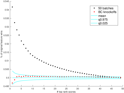
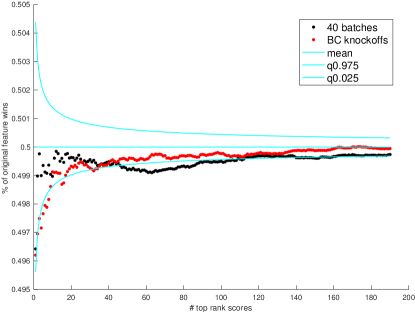
C. Uniform random batches ($d=1$)	D. $X$ is not extended ($d=3$)
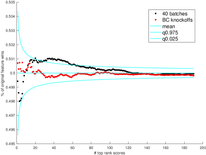
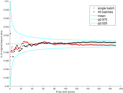
E. $X$ is extended ($d=3$)	F. $X$ is significantly extended

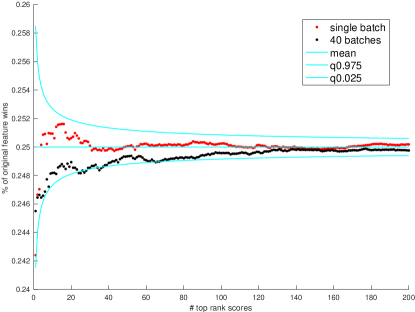
Figure 2: Examining the batched knockoff scores. Each panel examines the percentage of original feature wins among the top scoring true null features. If the knockoffs satisfy the conditional null exchangeability then those percentages can be modeled by the percentage of cumulative successes in an iid sequence of Bernoulli($c$) RVs. The cyan colored curves are the 0.975, 0.025 quantiles and the mean of the iid Bernoulli model. (A) The batched knockoffs exhibit a clear liberal bias when each batch consists of a single feature ($d=1$, $c=1/2$, $p=50$, $n=100$, $\Theta_{\rho}=I_{p}$, $K=1$, $A=10.0$, 60K datasets). (B-C) clustered batches (B) seem to follow the model more closely than the random uniform batches (C), which exhibit some distinct liberal bias ($d=1$, $c=1/2$, $p=200$, $n=800$, $\Omega_{\rho}$ with $\rho=0.7$, $K=10$, $A=2.8$, 40 batches, 50K datasets). (D) Comparing 40 clustered batches with non-batched knockoffs ($d=3$, $c=2/4$, $p=200$, $n=800$, $\Theta_{\rho}=I_{p}$, $K=10$, $A=2.8$, two distinct sets of 10K datasets). The design matrix $X$ was not extended. (E) Similar to panel E but the design matrix is extended by 200 rows of 0 ($d=3$, $c=1/4$, $p=200$, $n=600$, $\Theta_{\rho}=I_{p}$, $K=0$, two distinct sets of 10K datasets). (F) With $d=11$, $p=200$, $n=600$, we need to significantly extend $X$ (to $n=2400$) which in turn creates a liberal bias regardless of whether a single or 40 batches are used. The bias disappears once we use the known value of $\sigma=1$ rather than try to estimate it ($c=2/12$, $\Theta_{\rho}=I_{p}$, $K=0$, 40 batches, three distinct sets of 10K datasets).

Judging by panel A of Supp. Fig. 2 it seems that in this example where each batch consists of a single feature the resulting knockoffs exhibit a clear liberal bias: the percentage of original wins among the top true null features significantly exceeds our model-determined expected value of 1/2, as well as the variability we observed in Barber and Candès’ knockoffs. This bias further manifested itself in compromised FDR control. For example, applying our batched-knockoff+ (Section 5.3) we find that the empirical FDR at $\alpha=0.5$ is $0.5144$. This 3% overshoot of the empirical FDR might not seems that much, however our empirical FDR was computed from 60K independent samples so statistically it is a very significant deviation (8.8 standard deviations).

5.2.2 Clustering the features can help

In practice we found that with an average of five or more features per batch we avoid the significant bias observed in the example above. As mentioned, we partition the features into their batches by clustering them based on the similarities of the corresponding columns of the design matrix. This clustering based partition typically delivers only a modest improvement compared with an arbitrary uniform partition but there are cases where the difference can be significant. To see that we again consider the effect of batching on a single knockoff only now our emphasis is on the difference in percentage of target wins between these two types of partitions: uniform vs. clustering.

Specifically, we generated two sets of 50K datasets each with $p=200$, $n=800$, a covariance matrix $\Omega_{\rho}$ with $\rho=0.7$, $K=10$ features included in the model and an amplitude $A=2.8$. Each dataset’s features were partitioned into 40 batches but for the first 50K datasets we randomly and uniformly assigned 5 features to each batch while clustering was applied to define the batches of the subsequent 50K datasets.

Comparing panels B and C of Supp. Fig. 2 we see that while clustering based batching creates knockoffs for which the target wins percentage is in line with our model (panel B, black curve), the uniformly partitioned batches exhibit an undesirable significant liberal bias at some point (panel C, black). In both cases we added for reference the corresponding percentages we observe using Barber and Candès’ provably-reliable knockoffs.

5.2.3 Model-wise the batched multiple knockoffs behave similarly to their non-batched counterparts

In light of the above examples, and unless otherwise stated, our batched knockoffs were generated using clustering with an average of at least five features per batch. In this section we look specifically at the effect of batching on the agreement between the observed percentage of target wins among the true nulls and our model.

We begin with an example that did not require extending $X$: we generated two sets of 10K datasets, both with $p=200$, $n=800$, using an amplitude $A=2.8$, $K=10$ features included in the model and a covariance matrix $\Theta_{\rho}=I_{p}$ ($\rho=0$). We then compared the percentage of target wins using $d=3$ non-batched knockoffs with the same percentage when using $d=3$ knockoffs constructed using 40 batches. Panel D of Supp. Fig. 2 shows that in this case our batched knockoffs behave similarly to the un-batched ones. Notably, the latter are guaranteed to follow the model and indeed, in both cases the percentage of target wins does not deviate significantly from the theoretical $c=1/2$ (using $c=1/4$ yields qualitatively similar results).

The next example required extending $X$ because we constructed $d=3$ knockoffs as before but now $p=200$ and $n=600$ so $n<(d+1)p$. Again, we generated two sets of 10K datasets, one where the knockoffs were created using 40 batches per dataset and the other using a single batch per dataset. In this example all features were true null ($K=0$) and the covariance matrix was $\Theta_{\rho}=I_{p}$. Panel E of Supp. Fig. 2 shows that again our batched knockoffs behave similarly to the un-batched ones, and in both cases the percentage of target wins does not deviate significantly from the theoretical $c=1/4$ (using $c=1/2$ yields qualitatively similar results). Note that because $\boldsymbol{y}$ was extended using an estimate of $\sigma$ even the un-batched knockoffs are not guaranteed to follow the model in this case but in practice it seems they still do.

In our final example we look at a more significant extension of $X$ where we compared our knockoffs constructed in three different ways. For each of the three we generated 10K datasets using our model with $p=200$ and $n=600$, all features are true null ($K=0$) and a covariance matrix $\Theta_{\rho}=I_{p}$. Panel F of Supp. Fig. 2 shows that using 40 batches our $d=11$ knockoffs (black curve) demonstrate a clear liberal bias with $c=2/12$. Interestingly, when using a single batch to create the same number of $d=11$ knockoffs (red curve) we observe an even larger liberal bias than the one exhibited by the batched knockoffs (same value of $c=2/12$). This suggests that the issue lies with the fairly extreme extension we used rather than with the batching. Indeed, constructing our third set of knockoffs using the known $\sigma=1$, rather than its estimate, to extend $\boldsymbol{y}$ we note that the liberal bias has all but disappeared (green curve). Note that the three curves of Panel F were generated using the same $c=2/12$ but the results look qualitatively similar using other values of $c=i/12$ with $i\leq 6$. Regardless of the source of the above liberal bias we will show below that in practice it is sufficiently mild that it does not seem to obstruct our ability to control the FDR in the examples we looked at.

5.3 Assessing the knockoff selection procedures

We next investigate and compare the performance of our selection procedures by applying them to randomly drawn datasets. Specifically we considered:

• Barber and Candès’ knockoff+, that uses its own single knockoff construction, and “batched-knockoff+” which, like knockoff+, uses a single knockoff but in this case the knockoff is constructed using our batching procedure (so when the number of batches $b=1$ the two procedures are essentially equivalent though they can differ substantially when $b>1$).

• the recently proposed methods of mirror, max and LBM (Section 4.1).

• the new multi-knockoff and multi-knockoff-select that use a pre-specified number of model-aware bootstrap samples, $m_{b}$ (Section 4.2).

In Supp. Sec. 7.1 we provide the details of the settings that were used by these selection procedures (e.g., number of bootstrap samples).

We evaluated the performance of each method by noting its empirical FDR and power as we varied the FDR threshold. Specifically, for each combination of parameter values we randomly drew (typically) 1K datasets and for each considered FDR threshold $\alpha\in\Phi$ we averaged the FDP in the reported list of discoveries to get the empirical FDR, and we averaged the percentage of true features in the same list to get the average power.

We used three types of plots to visually study the selection methods we consider: power, power-difference and empirical FDR. Each plot is typically made of multiple curves, where each curve corresponds to a unique combination of parameter values. Specifically, each curve summarizes the results obtained by applying, at each considered FDR threshold, one or two of the methods to (typically) 1K datasets that were randomly drawn with the same given combination of parameter values, where:

• in a power plot ($y$-axis label indicates “Power”) each curve depicts a selection method’s average power over the randomly drawn datasets.

• in a power-difference plot ($y$-axis label indicates “Power Difference”) a curve represents the difference in average power between the first and second methods, so negative values indicate the second method is more powerful at the given FDR threshold.

• in an empirical FDR plot ($y$-axis label indicates “FDR”) the curve yields the ratio between the empirical FDR (average of the FDP) to the FDR threshold, so a value below 1 indicates a conservative bias and a value above 1 indicates a liberal bias.

5.3.1 Multiple-knockoff procedures that rigorously control the FDR in the finite sample case

Comparing the performance of knockoff+ with that of the multiple-knockoff procedures when all are guaranteed to control the FDR we see mixed results. Recall that such finite sample FDR control is guaranteed when the data is generated according to our model, we construct our $d\leq n/p-1$ knockoffs using a single batch and we apply our procedure with the mirandom map and pre-determined tuning parameters (e.g., the mirror and the max methods). Indeed, Theorem 1 here and Theorem 2 of [9] guarantee FDR control in this setting.

A. $n=3000,p=1000$; varying $A$ (amplitude)	B. $n=800,p=200$; varying $A$
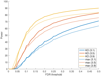
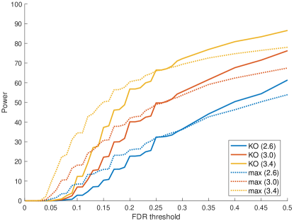
C. varying $\rho$ (feature correlation)	D. varying $\rho$
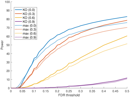
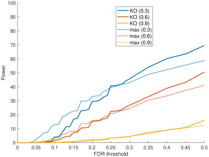
E. varying $K$ (# of features in model)	F. varying $K$;

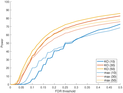
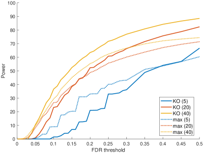
Figure 3: Power plots of knockoff+ (KO) and max in specific cases of guaranteed FDR control. Each left column panel gives the power of Barber and Candès’ single knockoff juxtaposed with the max procedure using two knockoffs ($n=3000,p=1000$ and unless explicitly varied, $k=30,\rho=0,A=3.5$, Supp. Sec. 7.1.2). The right column panels show knockoff+ and the max using three knockoffs ($n=800,p=200$ and unless explicitly varied, $k=10,\rho=0,A=3.0$, Supp. Sec. 7.1.1). (A) varying the amplitude: $A\in\left\{3.1,3.5,3.9\right\}$ . (B) varying the feature correlation strength of $\Theta_{\rho}$: $\rho\in\left\{0.0,0.3,0.6,0.9\right\}$. (C) varying the number of features, sparsity: $K\in\left\{10,30,50\right\}$. (D) varying the amplitude: $A\in\left\{2.6,3.0,3.4\right\}$. (E) varying $\Theta_{\rho}$’s $\rho$: $\rho\in\left\{0.0,0.3,0.6,0.9\right\}$. (F) varying $K\in\left\{5,20,40\right\}$. Overall max tends to do better for smaller FDR thresholds, sparser models and a larger $d$ but the results are mixed.

Figure 1 (A) shows that in some cases max delivers significantly more power than knockoff+ while in others it can deliver substantially less power. Supp. Fig. 3 offers more insight by showing how the power of max and knockoff+ vary with the parameters of the data and the FDR threshold. Overall max tends to do better for smaller FDR thresholds, sparser models and a larger $d$ but the results are generally mixed.

A. Max ($d=2,3$) vs. knockoff+	B. Empirical FDR (max)
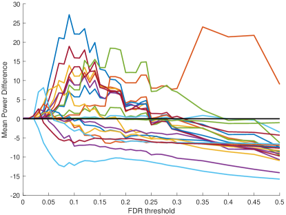
C. Mirror ($d=2,3$) vs. knockoff+	D. Empirical FDR (mirror)
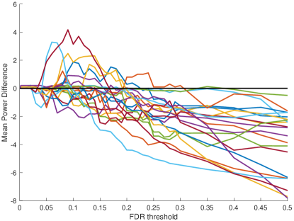
E. Batched-knockoff+ (1 batch) vs. knockoff+	F. Empirical FDR (batched-knockoff+)

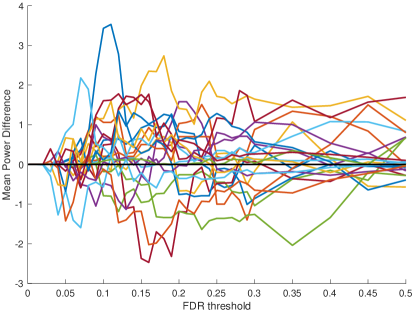
Figure 4: Comparison with knockoff+ and FDR control in guaranteed settings. The left column panels show the difference between the power of the considered method and knockoff+’ power (negative values indicate knockoff+ is more powerful at that threshold). The right column panels examine the ratio of the empirical FDR of the considered method (averaged over 1K runs) to the FDR threshold. The data for both columns consists of experiments in which all methods have guaranteed FDR control: $n=3000,p=1000,d=2,b=1$ (Supp. Sec. 7.1.2) and $n=800,p=200,d=3,b=1$ (Supp. Sec. 7.1.1). (B) There is a single (essentially random) spike at the FDR threshold of 0.001 (0.1%) where for that particular set of parameters from Supp. Sec. 7.1.2 the empirical FDR of max is just below 0.2% so it is almost 20% over the threshold. (E) batched-knockoff+ vs. knockoff+. As $b=1$ here the two methods are essentially equivalent so variations in power are essentially random. (F) batched-knockoff+ (knockoff+’ FDR plot is naturally quite similar to this one).

Supp. Fig. 4 shows a summary of the difference in power between max/mirror/batched-knockoff+ and knockoff+ (left column) as well as the empirical evidence of the corresponding FDR control (right column). Note that (a) because we use a single batch in this case, batched-knockoff+ is essentially equivalent to knockoff+ and the variations in power between them are random, and (b) mirror is much closer to knockoff+ here than max.

The guaranteed FDR control setup considered here is rather limited. In practice we would like to apply our methods to the case where $p<n<(d+1)p$. In addition, as we will see below, we can gain significant power by learning $c$ and $\lambda$ from the data, as well as by using batching when creating the knockoffs. We empirically explore these extensions next.

5.3.2 Batching can significantly increase the power of the knockoff procedures

A. Power of mirror ($n=600,p=200$)	B. FDR of mirror
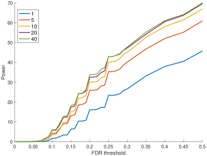
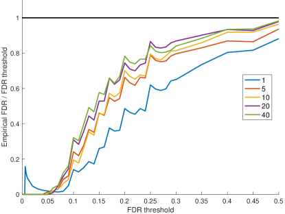
C. Power of batched-knockoff+	D. FDR of batched-knockoff+
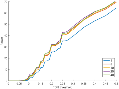
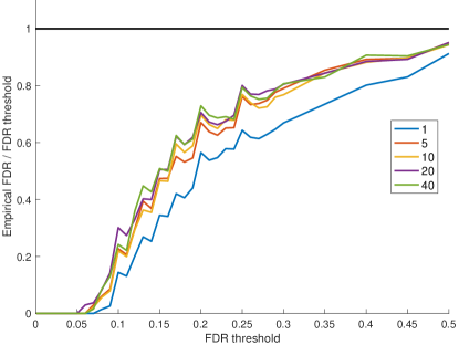
E. Power of knockoff+ (variations are random)	F. FDR of max

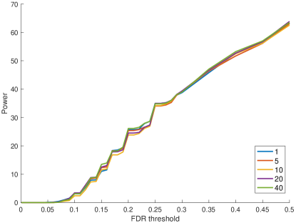
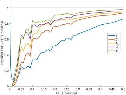
Figure 5: Power increases with the number of batches (I). Each of the left column panels shows the power of one method applied using a different number of batches $b\in\left\{1,5,10,20,40\right\}$ to construct the knockoffs. The design of the experiment involved randomly drawing a new set of 1K datasets with for each value of $b$ ($n=600,p=200$, Supp. Sec. 7.1.4). Each of the right column panels shows the ratio of the empirical FDR to the FDR threshold. (E) knockoff+ is not affected by the number of batches hence the observed power variations give us some idea on the magnitude of the differences due to the randomly generated datasets.

Panel B of Figure 1 as well as panels A-D of Supp. Fig. 5 show examples where, as expected, the power of our procedures generally increases with the number of batches because we are able to better distinguish the original features from their knockoffs.

A. Max using $b=1$ vs. $b=40$ batches	B. Mirror
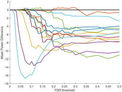
C. batched-knockoff+	D. knockoff+

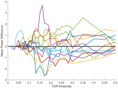
Figure 7: Batching increases the power (single vs. 40 batches). Each of the panels shows the difference in the power of one method applied to multiple datasets using $b=1$ ($n=800,p=200$, Supp. Sec. 7.1.1), and $b=40$ batches ($n=800,p=200$, Supp. Sec. 7.1.3). The design of the experiment involved drawing a new set of 1K datasets for each value of $b$. (D) knockoff+’ does not use batching so variations are simply due to the differences in the randomly drawn datasets.

Similarly, panel C of Figure 1 as well as Supp. Fig. 7 show in the context of the various datasets that make the $n=800,p=200,d=3$ set (Supp. Sec. 7.1.1) that increasing the number of batches from 1 to 40 typically yields substantial power gains. This holds for all three procedures we looked at so far: max, mirror and batched-knockoff+, and for the wide range of parameter combinations described in Supp. Sec. 7.1.1.

A. Max vs. knockoff+	B. Empirical FDR (max)
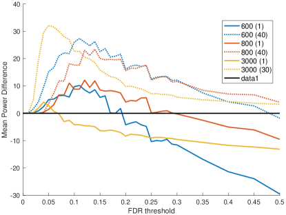
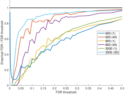
C. Mirror vs. knockoff+	D. Empirical FDR (mirror)
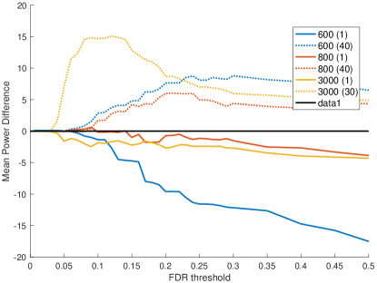
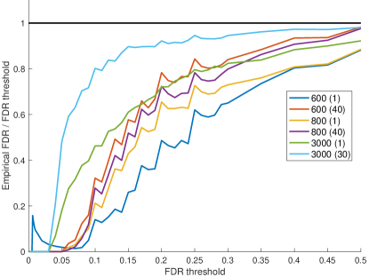
E. Batched-knockoff+ vs. knockoff+	F. Empirical FDR (batched-knockoff+)

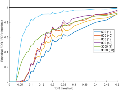
Figure 9: When the batching effect is more pronounced. Each of the left column panels shows the difference in the power of one method vs. knockoff+ applied using either $b=1$ or $b>1$ batches: $b=30$ for $n=3000,p=1000,K=30,A=3.5,d\in\left\{1,3\right\}$, and $b=40$ for $n=800,p=200,K=10,A=3.0,d\in\left\{1,3\right\}$, and for $n=600,p=200,K=10,A=2.8,d\in\left\{1,11\right\}$, $\rho=0$ in all cases, (Supp. Sec. 7.1.6) The design of the experiment involved drawing a new set of 1K datasets for each value of $b$ but knockoff+ and the method to which it is compared were applied to the same dataset each time. Negative values indicate knockoff+ is more powerful. Each right column panel uses the same datasets as the panel to its left to show the ratio of the empirical FDR of the considered method to the FDR threshold. The ratios are all below 1 indicating the methods seem to control the FDR in all these cases.

As expected, batching offers a larger increase in power as $d$ and $p$ increase. Some evidence of this can be seen in the left column panels of Supp. Fig. 9, which compare the power of max, mirror and batched-knockoff+ to the power of knockoff+ using $b=1$ and $b=40$ batches: the gains using $b=40$ are significantly larger when $p$ is increased from 200 to 1000 as well as when $d$ is increased from 3 to 11.

As mentioned in Sections 5.2.1 and 5.2.3 FDR control can be compromised when introducing batching, and particularly when a significant extension of $X$ and $\boldsymbol{y}$ is involved. Thus, we should examine whether the significant power gains we see in our examples when we introduce batching are not attained at the cost of compromised FDR control. Supp. Figs.  5 (right panels), 6 (right panels), 8, and 9 confirm that the FDR seems to be properly controlled in spite of the large power gains.

A. Max ($d=2,3$) knockoffs vs. knockoff+	B. Varying the number of batches (max)
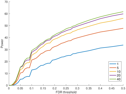
C. Max using $b=1$ vs. $b=40$ batches	D. LBM vs. multi-knockoff (combined dataset)
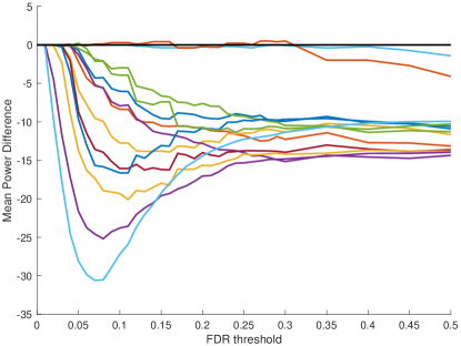
E. Varying $d$ (multi-knockoff)	F. knockoff+ vs. multi-knockoff-select (combined)

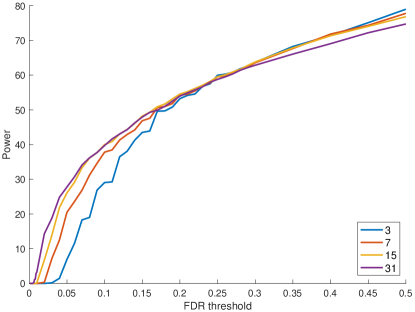
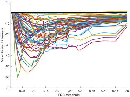
Figure 1: Main figure. (A) Power difference between knockoff+ and max using $d=2$ ($n=3000,p=1000$, Supp. Sec. 7.1.2) or $d=3$ ($n=800,p=200$, Supp. Sec. 7.1.1) knockoffs. (B) Power of max for varying number of batches $b\in\left[1,40\right]$ ($n=600,p=200,d=11,A=2.8$, Supp. Sec. 7.1.4). (C) Power difference between the max method using a single vs. 40 batches ($n=800,p=200,d=3$, Supp. Sec. 7.1.1) (D) Power difference: LBM vs. multi-knockoff on the combined dataset (Supp. Sec. 7.1.11). Negative values indicate multi-knockoff is more powerful. (E) Power of multi-knockoff for varying number of knockoffs $d\in\left\{1,3,7,15,31\right\}$ ($n=600$, $p=200$, $K=10$, $A=3.0$, $b=40$ dataset from the set described in Supp. Sec. 7.1.9). (F) Power difference between knockoff+ and multi-knockoff-select on the combined set (Supp. Sec. 7.1.11).

5.3.3 Empirically choosing the tuning parameters

A. LBM vs. multi-knockoff ($d\geq 7$)	B. LBM vs. multi-knockoff ($d\leq 3$)
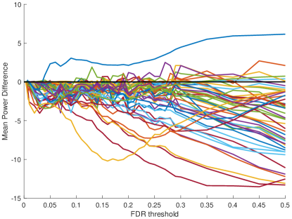
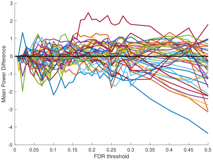
C. Empirical FDR (multi-knockoff)	D. Empirical FDR (LBM)

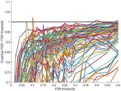
Figure 10: Multi-knockoff vs. LBM. Comparison of the two resampling-based methods for selecting the ($c,\lambda$) tuning parameters. Both methods were applied to all the datasets in our combined collection of experiments, which spans a wide range of parameter values and is described in Supp. Sec. 7.1.11. (A) Power difference between LBM and multi-knockoff (negative numbers mean multi-knockoff is better). Only experiments with $d\geq 7$ knockoffs are shown. The one example where LBM is moderately better than multi-knockoff (cyan colored) corresponds to a realistically borderline 80% proportion of features in the model: $K=160$ and $p=200$ ($n=600$, $d=11$). (B) Same as A but with $d\leq 3$ (same as $d<7$ in this case). (C-D) Empirical FDR on the entire “combined” set.

We first compare the performance of LBM, our general multiple-competition selection procedure, with that of multi-knockoff which is designed for this linear regression context. Specifically, we apply both methods to all the datasets in our combined collection of experiments, which spans the wide range of parameter values described in Supp. Sec.  7.1.11. Panel D of Figure 1 shows that the model-aware multi-knockoff generally offers more power than the general-purpose LBM does. More specifically, comparing panels A and B of Supp. Fig. 10 we find that the advantage of multi-knockoff becomes evident when the number of knockoffs is larger: for $d=3$ (panel B) we do not see much of a difference, which is expected given that in this case multi-knockoff considers only three possible combination of values for ($c,\lambda$).

When we rely on data-driven methods to set the values of $c$ and $\lambda$ we lose the theoretical guarantee of FDR control regardless of whether or not we use batching and/or extension. Resorting to simulation studies we find that in the same extensive set of experiments both LBM and multi-knockoff seem to essentially control the FDR (panels C and D of Supp. Fig. 10), so the advantage of multi-knockoff does not seem to come at the expense of controlling the FDR.

A. Knockoff+ vs. multi-knockoff	B. Batched-knockoff+ vs. multi-knockoff
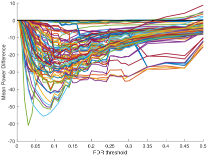
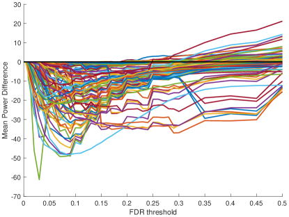
C. Mirror vs. multi-knockoff	D. Max vs. multi-knockoff
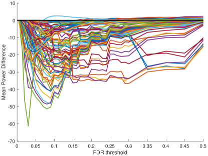
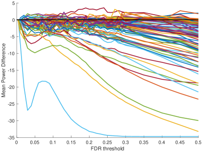
E. LBM vs. multi-knockoff	F. Multi-knockoff-select vs. multi-knockoff

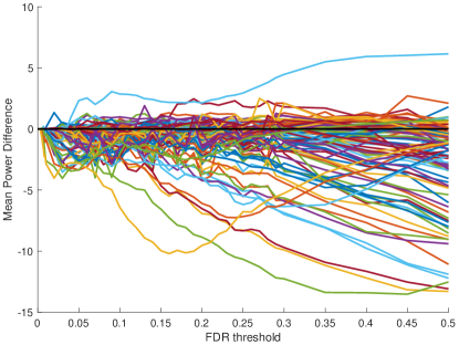
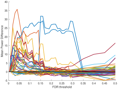
Figure 11: Power difference vs. multi-knockoff. Each panel shows the difference in power between one of the methods considered in this paper and multi-knockoff. All the methods were applied to all the datasets that are included the combined set described in Supp. Sec. 7.1.11. Note that the scale of the $y$-axis varies across the panels.

With multi-knockoff’s optimization of the tuning parameters ($c,\lambda$) apparently being better than LBM’s we went ahead and also compared the former’s power against all the other methods we consider here. Panels A-D of Supp. Fig. 11 show that in each case multi-knockoff is overall a better option: more often than not it delivers more power than each of the other methods, and moreover, when it is not optimal it is giving up only a small amount of power (certainly for the more practical FDR thresholds of $\alpha\leq 0.3$), while often enjoying a substantial advantage in power when it is optimal.

5.3.4 Choosing the optimal number of knockoffs

A. The optimal # of knockoffs, $d$, varies (max)	B. The optimal $d$ varies (multi-knockoff)
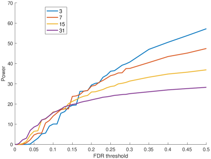
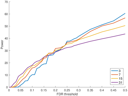
C. Same as B but with multi-knockoff-select	D. multi-knockoff vs. multi-knockoff-select
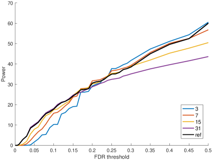
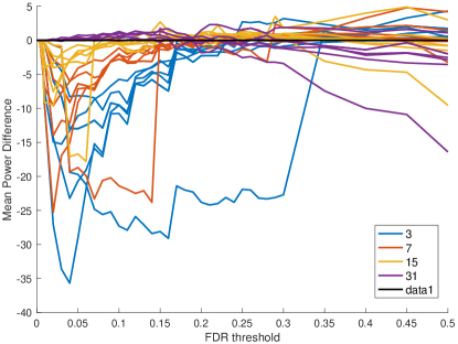
E. knockoff+ vs. multi-knockoff-select	F. Empirical FDR (multi-knockoff-select)

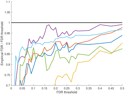
Figure 12: Varying the number of knockoffs All the plots were created using the set of experiments defined in Supp. Sec. 7.1.9. When applying any multiple-knockoff selection method to a randomly drawn dataset we used the increasing sequence of $d=3,7,15,31$ knockoffs so we can examine how the method’s power varies with $d$. (A-B) The optimal value of $d$ varies for the max method and multi-knockoff in this example where $n=600$, $p=200$, $K=10$ with $A=3.0$ and 0 feature correlation $\Theta_{0}=I_{p}$. (C) multi-knockoff-select (black “ref” curve) seems to do a good job at tracking the near-optimal value of $d$ (same data as in panel B). (D) The difference in average power of multi-knockoff vs. multi-knockoff-select using all six datasets in Supp. Sec. 7.1.9. (E) Same as in panel D but now the comparison is with knockoff+, which is evidently uniformly weaker than multi-knockoff-select. (F) Empirical evidence that multi-knockoff-select controls the FDR when applied to these datasets (same legend as panel E).

So far we examined the performance of the methods when the number of knockoff copies $d$ is given. However, it is not clear how to choose an optimal value of $d$ as the setup here is quite different to the iid decoys model that Emery et al. looked at. In the latter case, the larger $d$ is the more power the multiple-decoy procedure will generally deliver, however in our linear regression context there is a delicate balance between the increased power due to the increasing number of competing knockoffs and the reduction in power due to increased correlation between the knockoffs and the original features. Panels E of Figure 1 and A and B of Supp. Fig. 12 demonstrate this problem: the optimal number of knockoffs varies with the method we use, the parameters of the problem, and the FDR threshold. This was the motivation behind our new multi-knockoff-select that tries to optimally select $d$ from the choices it is given, so how well is it doing in practice?

Panels C and D of Supp. Fig. 12 show that in the case of the experiments described in Supp. Sec. 7.1.9 multi-knockoff-select seems to consistently select a nearly optimal $d$: in the studied cases its power for any $\alpha\leq 0.5$ was at worst 5% below the power of multi-knockoff applied with the optimal $d$ and the power difference was even smaller for $\alpha\leq 0.2$. At the same time, for each fixed $d$ there are settings where multi-knockoff-select delivers significantly more power than multi-knockoff. Importantly, the overall performance of multi-knockoff-select on this set generated using six different combinations of parameter values (Supp. Sec. 7.1.9) was uniformly better than Barber and Candès’s knockoff+ procedure for $\alpha\leq 0.5$ and often by a significant power margin (panel E, Supp. Fig. 12). At the same time, panel F of the same figure shows that this increase in power was not the result of compromised FDR control.

A. Knockoff+ vs. multi-knockoff-select	B. Batched-knockoff+ vs. multi-knockoff-select
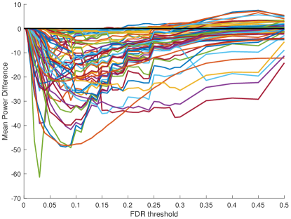
C. Mirror vs. multi-knockoff-select	D. Max vs. multi-knockoff-select
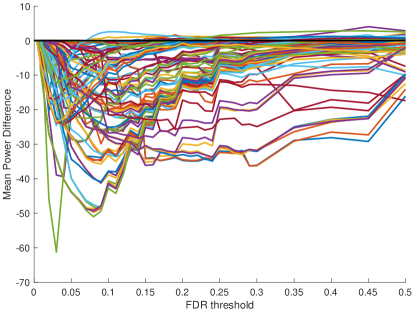
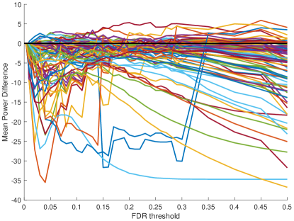
E. LBM vs. multi-knockoff-select	F. Multi-knockoff vs. multi-knockoff-select

Figure 13: Power difference vs. Multi-knockoff-select. Each panel shows the difference in power between one of the methods considered in this paper and multi-knockoff-select. All the methods were applied to all the datasets that are included the combined set described in Supp. Sec. 7.1.11. Note that the scale of the $y$-axis varies across the panels.

A. Empirical FDR (multi-knockoff-select)	B. Knockoff+ vs. multi-knockoff-select
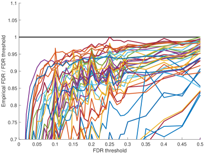
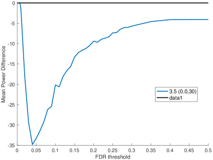
C. Empirical FDR (multi-knockoff-select)

Figure 14: More on multi-knockoff-select. (A) The FDR of multi-knockoff-select is empirically controlled on the wide set of parameter values of the combined set (Supp. Sec. 7.1.11). (B) Multi-knockoff-select (with $d\in\left\{1,3,7\right\}$ and $b=50$ batches) is uniformly more powerful than knockoff+ on the $n=3000$, $p=1000$, $K=30$, $A=3.5$, $\Theta_{0}=I_{p}$ example of [1]. (C) Empirical FDR of multi-knockoff-select on the same data used in panel B.

Moving on to our more extensive set of experiments described in Supp. Sec. 7.1.11 we find that multi-knockoff-select’s flexibility of optimizing over $d$ makes it our overall preferred procedure. Indeed, Supp. Fig. 13 shows that compared with any of the other methods we consider here multi-knockoff-select overall offers more power. In particular, panel A of Supp. Fig. 13 (for convenience it is the same as panel F of Figure 1) shows that multi-knockoff-select essentially uniformly delivers more power than knockoff+ and often significantly more. At the same time we again find that this increase in power does not come at the expense of our ability to control the FDR (panel A of Supp. Fig. 14).

Finally, it is instructive to take a closer look at the main example Barber and Candès considered of $n=3000$, $p=1000$, $K=30$, $A=3.5$, and 0 feature correlation $\Theta_{0}=I_{p}$. If we use $b=50$ batches to construct $d\in\left\{1,3,7\right\}$ knockoffs then even with only $m_{b}=4$ bootstrap multi-knockoff-select is a very computationally demanding procedure (about 11 hours per run on a 3.2GHz macMini). Fortunately, this significant computational effort is rewarded as we can see when comparing the power of multi-knockoff-select to that of knockoff+ (panel B of Supp. Fig. 14), and again FDR is well under control (panel C of same figure).

6 Discussion

When introducing their knockoff+ procedure Barber and Candès noted that using multiple knockoff copies could increase the power of their approach. We recently introduced a general approach to multiple competition-based FDR control and here we show how the two concepts could be merged. We first generalize the knockoff construction of Barber and Candès to generate $d$ knockoff copies and prove that under certain conditions (no extension of $X$, no batching and using pre-determined tuning parameters ($c,\lambda$)), applying our competition-based selection method to these multiple knockoffs rigorously controls the FDR in the finite sample setting.

Our initial knockoff construction is limited both in terms of its applicability ($n\geq(d+1)p$) and its utility (panel A of Figure 1). To address these issues we combine Barber and Candès’ extension notion with our proposed batching heuristic, and we empirically show that these revised knockoffs still allow us to effectively control the FDR in the variable selection problem while delivering a substantial increase in power.

Our recommended general procedure for controlling the FDR using multiple competition is constrained by the generic resampling technique it uses. Here we show that using a resampling scheme that is specifically adjusted to the linear regression context allows us to offer more powerful selection methods. Indeed, our multi-knockoff-select procedure is largely successful not only in setting a near-optimal value of ($c,\lambda$), the tuning parameters of our general FDR controlling procedure, but also in selecting an optimal number of knockoff copies. The latter is a non-trivial optimization problem due to the inherent conflict between the advantage that increasing $d$ offers in terms of the competition and the reduced power for each knockoff ($s_{0}$ is decreasing as $d$ is increasing).

While there are alternative procedures for controlling the FDR in the associated variable selection problem (e.g. [18, 19, 11, 17, 16]), Barber and Candès note that those, and for that matter their own knockoff (in contrast with their knockoff+) procedure, generally only asymptotically guarantee FDR control. They further demonstrate that among the procedures that control the FDR in the finite setting of the variable selection problem, their knockoff+ seems to be the most powerful one. Multi-knockoff-select is more powerful than knockoff+, allowing us to identify more truly associated features, while empirically we see that it maintains control of the rate of falsely discovered features even in the finite setting. It does however come at a substantial computational cost as well as of using a mathematically unproved technique.

A. $\rho=0$	B. $\rho=0.5$
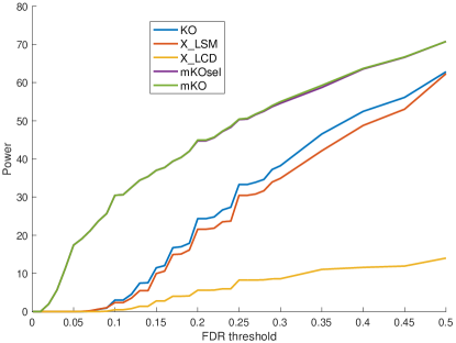
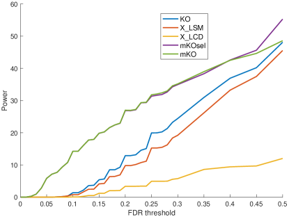
C. $\rho=0.9$	D. Empirical FDR ($\rho=0$)

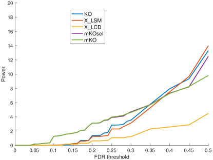
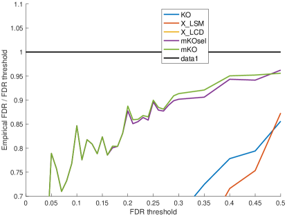
Figure 15: Comparison with model-X knockoffs. In this figure we examine the performance of the model-X knockoffs. The data consisted of $n=600$, $p=200$, $K=10$, $A=2.8$ and a varied feature correlation strength as described in Supp. Sec. 7.1.12. (A-C) The model-X LSM is on-par or below knockoff+ while the model-X LCD is generally significantly behind both. At the same time multi-knockoff and multi-knockoff-select dominates the single knockoff methods except when the FDR threshold is $\geq 0.35$ and the feature correlation is very high ($\rho=0.9$). (D) For this case of $\rho=0$ the empirical FDR of LCD is always below 70% of the threshold hence it does not appear in the plot. Similarly, for $\rho=0.5,0.9$ the empirical FDR of all the methods was consistently significantly below the threshold so we omitted those figures.

We concentrated on comparing our multiple-knockoff methods with knockoff+ because they naturally generalize that method but it is also instructive to consider the more recent model-X knockoffs [5]. The model-X knockoffs are designed for a different variant of the linear regression problem where the design matrix itself is also drawn according to some known distribution. This assumption is still consistent with the setup of our simulations so we compared the performance of the model-X knockoffs with the other knockoff procedures in a couple of examples (Supp. Sec. 7.1.12). Supp. Fig. 15 suggests that in the context of our simulations the model-X lasso signed max (LSM) statistic was roughly on-par or slightly weaker than the original knockoff+, and the model-X lasso coefficient difference (LCD) statistic significantly lagged behind those two. In particular, unless the FDR threshold was relatively high and the feature correlation extremely high ($\rho=0.9$), all these single-knockoff methods offered significantly less power than multi-knockoff-select.

There are a few directions we would like to explore following this work. First, like the original knockoff+ our method is limited to the case $n>p$. Thus, it would be particularly interesting to see whether our approach can be combined with Barber and Candès’ recent extension to the $n\leq p$ case based on their data-splitting technique coupled with their introduction of a two step procedure: acquiring a partial model with $n>p$ and performing the knockoff procedure on the partial model [2]. Second, in this work we focused on generalizing the original knockoff construction to multiple knockoffs so an obvious question is how much of this carries over to the model-X knockoffs. Third, our current estimate of the noise level $\sigma$ is rather naive and, as we saw, using it the knockoff scores gradually drift from the assumed model when using large extensions (Section 5.2.1). It would therefore be interesting to explore more sophisticated estimations of $\sigma$ such as the one in [21].

7 Supplementary Material

7.1 Simulation setup

Our general simulation setup is described in Section 5.1. In the following sections we give further details about the parameter settings we used in our experiments in generating the original design matrices (and the response variables) and the knockoff features as well as any optional settings of our selection methods. When generating the data we varied the dimension of the design matrix $X$, $n\times p$, the number of true features, $K$, the signal amplitude $A$, and the feature correlation strength $\rho$ while keeping the variance of the noise fixed at $\sigma^{2}=1$ (cf. (1) and Section (5.1)). We generally randomly sampled 1K sets of data for each of the parameter combinations we considered and constructed a set of original plus $d$ knockoff scores for each feature using the specified number of $b$ batches.

While knockoff+ and batched-knockoff+ were each applied only once to the data — each with its corresponding knockoff — the multiple knockoff procedures were applied separately for each considered value of $d$ (with the knockoffs also separately constructed for each value of $d$, cf. Section 4.3).

Following knockoff+ we also use the glmnet implementation of the Lasso [20]. We found that the set of values the regularization parameter lambda is allowed to assume can have a non-negligible effect on our analysis. This is not surprising given that the original and the knockoff feature score corresponds to the largest value of lambda for which the coefficient of that feature is non-zero. Therefore, to make sure that the differences we observe between the methods are not due to variations in the number of lambdas, we set each method to use the same number of possible lambda values. Specifically, this number was set to $5\cdot\left(1+d_{\max}\right)\cdot p$ (we experimented a little with coefficients other than 5 but kept it at 5 throughout the simulations described here), where $d_{\max}$ is the maximal value of $d$ considered in that experiment. Importantly, it means that knockoff+ also used that maximal number of lambdas even though it is using a single knockoff.

In the same vein, we found that our knockoffs are better behaved if all our batches use the same set of lambdas. Specifically, we use the same exponentially spaced set of lambda values that knockoff+ uses only we set the maximal value to $\max_{i}\boldsymbol{x}_{i}^{T}\boldsymbol{y}/n$ where $\boldsymbol{x}_{i}$ varies over the columns of all augmented design matrices $\left[X\tilde{X}^{I_{j}}\right]$ (Section 3). Note that when using a single batch this maximal value coincides with the one originally used in the knockoffs package.

Somewhat more surprising was the fact that permuting the columns of the extended design matrix before applying glmnet also occasionally had a substantial effect on the performance of the FDR controlling methods, including on knockoff+. Therefore, we uniformly randomly permuted all extended design matrices.

Note that we applied LBM exactly as described in Supp. Sec. 6.6 of [9] and that when multiple number of knockoffs are considered in the same run the data is only resampled once using the largest considered number of knockoffs to create the model-aware resamples.

7.1.1 $n=800$, $p=200$, $d\in\left\{1,3\right\}$, $b=1$

A set of experiments designed to study the performance of FDR control with multiple knockoffs in the setting of guaranteed finite sample control. Each drawn dataset was generated starting with randomly drawing the $n\times p$ design matrix $X$ where $n=800$ and $p=200$ while varying the following parameters (drawing 1K independent datasets per each setting of the parameters):

• the number of true features $K$ (model sparsity): $K=1,5,10,20,40,80$ with $A=3.0$ and 0 feature correlation $\Theta_{0}=I_{p}$.

• the signal amplitude $A=2.6,2.8,3.0,3.2,3.4$ with $K=10$ and 0 feature correlation $\Theta_{0}=I_{p}$.

• the feature correlation strength $\rho=0,0.3,0.6,0.9$ of the Töeplitz correlation matrix $\Theta_{\rho}$ with $K=10$, $A=3.0$.

When analyzing each of these datasets we constructed three sets of knockoffs (cf. Section 4.3): the first with a single knockoff per feature as part of running knockoff+’, the second using our procedure to construct $d=1$ knockoff (for use in batched-knockoff+), and the third using our construction of $d=3$ knockoffs. Note that in this case we used a single batch so while our construction of $d=1$ knockoff is in practice different from knockoff+’ it is mathematically equivalent to it. In particular, knockoff+ and batched-knockoff+ are essentially equivalent.

7.1.2 $n=3000$, $p=1000$, $d\in\left\{1,2\right\}$, $b=1$

Similar in design and intent to the last section except that we used the same dimensions of the data as used in the introduction of knockoff+ [1] and varied:

• the number of true features $K$ (model sparsity): $K=0,30,50$ with $A=3.5$ and 0 feature correlation $\Theta_{0}=I_{p}$.

• the signal amplitude $A=3.1,3.5,3.9$ with $K=30$ and 0 feature correlation $\Theta_{0}=I_{p}$.

• the feature correlation strength $\rho=0,0.3,0.6,0.9$ with $K=30$, $A=3.5$.

For each of these combinations of parameters we drew 1K datasets and constructed two sets of knockoffs, each using a single batch, one with $d=1$ (again equivalent to knockoff+’ single knockoff) and another with $d=2$ knockoffs per feature.

7.1.3 $n=800$, $p=200$, $d\in\left\{1,3\right\}$, $b=40$

In this set of experiments we largely repeated the setup described in Supplementary Section (7.1.1) above with the major difference that we used 40 batches when constructing either $d=1$ or $d=3$ knockoffs per feature rather than a single batch. In particular, here batched-knockoff+ substantially differs from knockoff+.

Also, in addition to generating 1K datasets for each of the parameter combinations described above we generated additional 1K datasets per parameter combination while varying:

• the number of true features $K=1,5,10,20,40,80$ with $A=2.8$ and 0 feature correlation $\Theta_{0}=I_{p}$.

• the feature correlation strength $\rho=0,0.3,0.6,0.9$ with $K=10$, $A=2.8$.

Applications of multi-knockoff and multi-knockoff-select used $m_{b}=32$ model-aware bootstrap samples.

7.1.4 $n=600$, $p=200$, $d\in\left\{1,11\right\}$, $b\in\left\{1,5,10,20,40\right\}$

A set of experiments designed to demonstrate the effects that increasing number of batches can have. The datasets were generated using a fixed $600\times 200$ dimension for the design matrix, with $A=2.8$ and 0 feature correlation $\Theta_{0}=I_{p}$. For each $b\in\left\{1,5,10,20,40\right\}$ we randomly generated 1K datasets, then using $b$ batches each time we constructed two sets of knockoffs one with $d=1$ and another with $d=11$ knockoffs per feature. Applications of multi-knockoff and multi-knockoff-select used $m_{b}=32$ model-aware bootstrap samples.

7.1.5 $n=3000$, $p=1000$, $d\in\left\{1,3\right\}$, $b\in\left\{1,5,10,30,50\right\}$

Similar in design and intent to the last section except that (a) we used different parameter values, and (b) when creating these sets of knockoffs we did not use clustering when defining the batches, instead we arbitrarily divided the features into equal sized batches (which of course is irrelevant for $b=1$).

Applications of multi-knockoff and multi-knockoff-select used $m_{b}=4$ model-aware bootstrap samples.

7.1.6 “Eclectic batching example”

This set gathered together some specific experiments for demonstrating the effects of batching on larger examples. It consisted of three pairs of experiments:

• $n=800,p=200,d\in\left\{1,3\right\},b\in\left\{1,40\right\}$ taken from Supp. Secs. 7.1.1 and 7.1.3.

• $n=600,p=200,d\in\left\{1,11\right\},b\in\left\{1,40\right\}$ taken from Supp. Sec. 7.1.4.

• $n=3000,p=1000,d\in\left\{1,3\right\},b\in\left\{1,30\right\}$ taken from Supp. Secs. 7.1.2 and 7.1.10.

7.1.7 $n=800$, $p=200$, $d\in\left\{1,3,7\right\}$, $b=40$

In this set of experiments we used the same parameter combinations for generating the data as described in Supplementary Section 7.1.1 above. The difference again was in the analysis stage where here we constructed for each drawn design matrix $X$ three sets of knockoffs (in addition to the set generated by knockoff+). Each set was constructed using 40 batches: one with $d=1$, another with $d=3$ and the third with $d=7$ knockoffs per feature. We then applied knockoff+ and batched-knockoff+ using their corresponding single knockoff set, and we applied each of the multiple-knockoff procedures twice, once to the $d=3$ set and once to the $d=7$ set. Applications of multi-knockoff and multi-knockoff-select used $m_{b}=32$ model-aware bootstrap samples.

7.1.8 $n=600$, $p=200$, $d\in\left\{1,11\right\}$, $b=40$

In this set of experiments we used a larger number of knockoffs with $600\times 20$0 design matrices. Again, we generated 1K datasets (design matrix and response variables) for each of the following combinations of parameters, varying:

• the number of true features $K=0,1,5,10,20,40,80,160$ with $A=2.8$ and 0 feature correlation $\Theta_{0}=I_{p}$.

• the signal amplitude $A=2.4,2.6,2.8,3.0,3.2$ with $K=10$ and 0 feature correlation $\Theta_{0}=I_{p}$.

• the feature correlation strength $\rho=0,0.3,0.5,0.7,0.9$ of the Töeplitz correlation matrix $\Theta_{\rho}$, as well as using $\rho=0.5$ for $\Omega_{\rho}$ (constant $\rho$ on the off-diagonal terms) with $K=10$, $A=2.8$.

Note that for two of the experiments we increased the number of runs to 4K from the initial 1K by adding another 3K independent runs to clarify whether the relatively high empirical FDR that was observed in a couple of the settings was significant. In both cases $(K=5$ and $K=0$) the aggregated 4K runs did not show a substantial FDR violation. For each drawn dataset we used $b=40$ batches to construct two sets of knockoffs, one with a single knockoff per feature, and another with $d=11$.

7.1.9 $n=600$, $p=200$, $d\in\left\{1,3,7,15,31\right\}$, $b=40$

This set of experiments was specifically designed to compare the performance using a varying number of knockoffs while analyzing the same data, as well as to test the ability of multi-knockoff-select to select an optimal number of knockoff. Each of the following combination of parameters was used to generate 1K datasets and for each we constructed a knockoff set for each value of $d\in\left\{1,3,7,15,31\right\}$ using $b=40$ batches per construction (in addition to the knockoffs generated by knockoff+). To generate the data we varied:

• the number of true features $K$ (model sparsity): $K=1,10,40$ with $A=3.0$ and 0 feature correlation $\Theta_{0}=I_{p}$.

• the signal amplitude $A=2.6,3.0,3.4$ with $K=10$ and 0 feature correlation $\Theta_{0}=I_{p}$.

• the feature correlation strength $\rho=0,0.5$ of $\Theta_{\rho}$ with $K=10$, $A=3.0$.

Applications of multi-knockoff and multi-knockoff-select used $m_{b}=32$ model-aware bootstrap samples.

7.1.10 $n=3000$, $p=1000$, $d\in\left\{1,3\right\}$, $b=30$

The data for this set of experiments was generated using the same general parameter settings as those used in the simulation part of [1]. Specifically, we drew $3000\times 1000$ design matrices and response variables by varying:

• the number of true features $K$ (model sparsity): $K=0,5,10,30,50,75,100,200$ with $A=3.5$ and 0 feature correlation $\Theta_{0}=I_{p}$.

• the signal amplitude $A=2.7,3.1,3.5,3.9,4.3$ with $K=30$ and 0 feature correlation $\Theta_{0}=I_{p}$.

• the feature correlation strength $\rho=0,0.3,0.5,0.7,0.9$ of the Töeplitz correlation matrix $\Theta_{\rho}$, as well as using $\rho=0.5$ for $\Omega_{\rho}$ (constant $\rho$ on the off-diagonal terms) with $K=30$, $A=3.5$.

For each of these combinations of parameters we drew 1K datasets and constructed two sets of knockoffs, one with $d=1$ and another with $d=3$ knockoffs per feature, using $b=30$ batches each time.

Applications of multi-knockoff and multi-knockoff-select used $m_{b}=4$ model-aware bootstrap samples.

7.1.11 Combined dataset

The “combined dataset” was created by merging together the $n=3000,p=1000$ sets (Supp. Sec. 7.1.10), the $n=800,p=200$ sets (Supp. Secs. 7.1.3 and 7.1.7 but keeping only one copy of each duplicated $d=3$ set), and the $n=600,p=200$ sets (Supp. Secs. 7.1.8 and 7.1.9).

7.1.12 The model-X dataset

We used this data to compare against the newer model-X knockoffs of [5]. The design matrix was $n=600$ by $p=200$, the model had $K=10$ features with $A=2.8$ and we only varied the feature correlation $\rho=0.0,0.5,0.9$ while creating $d=11$ knockoffs using $b=40$ batches. Applications of multi-knockoff and multi-knockoff-select used $m_{b}=32$ model-aware bootstrap samples. The model-X knockoffs were created as follows:

• The knockoff features were created using the create function of the Matlab knockoffs package [5] with the model defined as gaussian coupled with the mean and covariance estimated from the randomly drawn design matrix $X$ using the Matlab functions mean and cov. We used the “equicorrelated” construction because our knockoff construction also uses the same constant $s_{0}$ construction.

• We generated the model-X Lasso signed max (LSM) statistic using a slightly modified version of the function lassoLambdaSignedMax from the knockoffs package that enabled us to to randomly permute the order of the columns of the extended design matrix (see Supp. Sec. 7.1). We set the function’s nlambda parameter to the same value that the other methods were using (see Supp. Sec. 7.1).

• We generated the model-X Lasso coefficient difference (LCD) statistic using a similarly modified version of the lassoCoefDiff function from the knockoffs package that allowed us to randomly permute the extended design matrix columns but other than that we used all the default settings of the original function.

7.1.13 The set $\Phi$ of FDR thresholds

For computational efficiency we evaluated the power and empirical FDR of each of the considered procedures on a pre-determined set of possible FDR thresholds. Specifically we used the set of FDR thresholds $\Phi$: from 0.001 to 0.009 by jumps of 0.001, from 0.01 to 0.29 by jumps of 0.01, and from 0.3 to 0.95 by jumps of 0.05. Our figures however only extend to an FDR threshold of 0.5 since in practice FDR thresholds higher than 50% are typically of little importance.

7.2 Figures

A. Power of max ($n=3000,p=1000$)	B. FDR of max
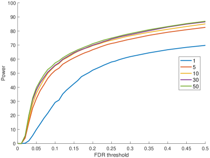
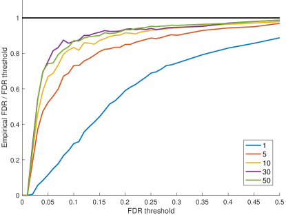
C. Power of batched-knockoff+	D. FDR of batched-knockoff+
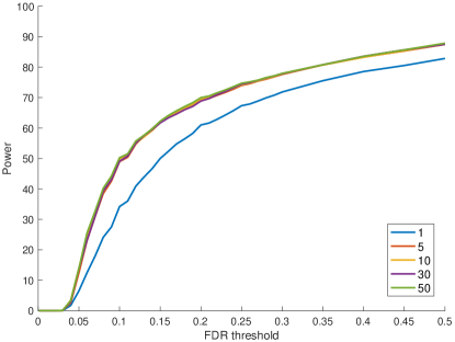
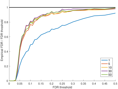
E. Power of knockoff+ (variations are random)	F. FDR of mirror

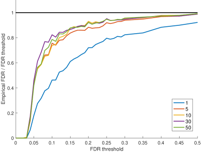
Figure 6: Power increases with the number of batches (II). Same as Supp. Fig. 5 except $b\in\left\{1,5,10,30,50\right\}$ and $n=3000,p=1000$ (Supp. Sec. 7.1.5).

A. Empirical FDR (max)	B. Empirical FDR (mirror)
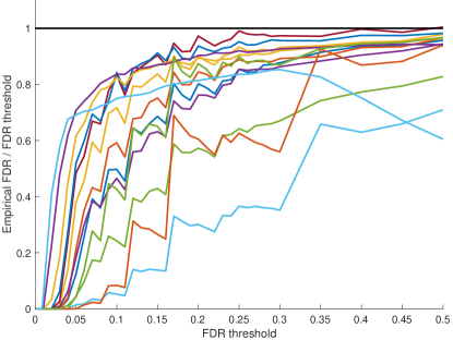
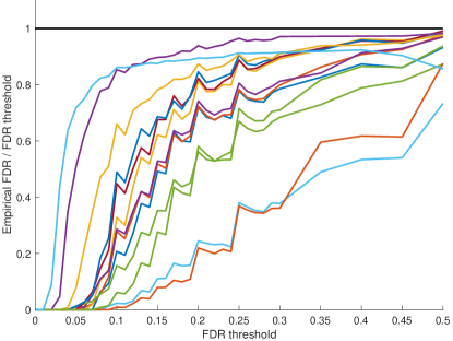
C. Empirical FDR (batched-knockoff+)	D. Empirical FDR (knockoff+)

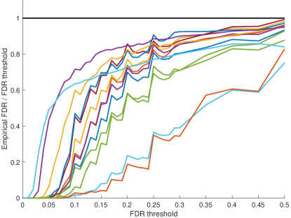
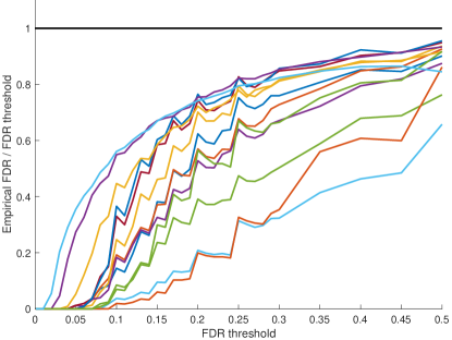
Figure 8: Batching does not seem to compromise the finite sample FDR control. Each of the panels shows the ratio of the empirical FDR to the FDR threshold of one method applied to multiple datasets using $b=40$ batches ($n=800,p=200$, Supp. Sec. 7.1.3). The graphs show that in all the cases the methods seem to essentially control the FDR. (D) knockoff+’ control of the FDR is guaranteed in this setting where $n\geq 2p$.

References

- [1] R. F. Barber and Emmanuel J. Candés. Controlling the false discovery rate via knockoffs. The Annals of Statistics, 43(5):2055–2085, 2015.
- [2] R. F. Barber and Emmanuel J. Candés. A knockoff filter in high-dimensional selective inference. ArXiv, 2016.
- [3] Rina Foygel Barber and Emmanuel J. Candes. Controlling the false discovery rate via knockoffs. Ann. Statist., 43(5):2055–2085, 10 2015.
- [4] Y. Benjamini and Y. Hochberg. Controlling the false discovery rate: a practical and powerful approach to multiple testing. Journal of the Royal Statistical Society Series B, 57:289–300, 1995.
- [5] Emmanuel J Candès, Yingying Fan, Lucas Janson, and Jinchi Lv. Panning for gold: Model-X knockoffs for high-dimensional controlled variable selection. Journal of the Royal Statistical Society Series B, 2018. to appear.
- [6] Fabio R. Cerqueira, Armin Graber, Benno Schwikowski, and Christian Baumgartner. Mude: A new approach for optimizing sensitivity in the target-decoy search strategy for large-scale peptide/protein identification. Journal of Proteome Research, 9(5):2265–2277, 2010.
- [7] J. E. Elias and S. P. Gygi. Target-decoy search strategy for increased confidence in large-scale protein identifications by mass spectrometry. Nature Methods, 4(3):207–214, 2007.
- [8] J. E. Elias and S. P. Gygi. Target-decoy search strategy for mass spectrometry-based proteomics. Methods in Molecular Biology, 604(55–71), 2010.
- [9] K. Emery, S. Hasam, W. S. Noble, and U. Keich. Multiple competition-based FDR control for peptide detection. arXiv, 2019. arXiv:1907.01458v2.
- [10] G. H. Golub and C. F. Van Loan. Matrix Computations. Johns Hopkins, 3rd edition, 1996.
- [11] M. G’Sell, S. Wager, A. Chouldechova, and R. Tibshirani. Sequential selection procedures and false discovery rate control. Journal of the Royal Statistical Society. Series B (Statistical Methodology), 78(2):423–444, 2016.
- [12] Gareth James, Daniela Witten, Trevor Hastie, and Robert Tibshirani. An introduction to statistical learning, volume 112. Springer, 2013.
- [13] K. Jeong, S. Kim, and N. Bandeira. False discovery rates in spectral identification. BMC Bioinformatics, 13(Suppl. 16):S2, 2012.
- [14] U. Keich and W. S. Noble. Progressive calibration and averaging for tandem mass spectrometry statistical confidence estimation: Why settle for a single decoy. In S. Sahinalp, editor, Proceedings of the International Conference on Research in Computational Biology (RECOMB), volume 10229 of Lecture Notes in Computer Science, pages 99–116. Springer, 2017.
- [15] U. Keich, K. Tamura, and W. S. Noble. Averaging strategy to reduce variability in target-decoy estimates of false discovery rate. Journal of Proteome Research, 18(2):585–593, 2018.
- [16] H. Liu, K. Roeder, and L. Wasserman. Stability approach to regularization selection (stars) for high dimensional graphical models. Advances in neural information processing systems, 24(2):1432–1440, 2010.
- [17] N. Meinshausen and P. Bühlmann. Stability selection. Journal of the Royal Statistical Society. Series B (Statistical Methodology), 72:417–473, 2010.
- [18] A. Miller. Subset Selection in Regression. Chapman & Hall/CRC Monographs on Statistics & Applied Probability. CRC Press, 2nd edition, 2002.
- [19] A. J. Miller. Selection of subsets of regression variables. Journal of the Royal Statistical Society. Series A (General), 147(3):389–425, 1984.
- [20] J. Qian, T. Hastie, J. Friedman, R. Tibshirani, and N. Simon. Glmnet for matlab, 2013.
- [21] Stephen Reid, Robert Tibshirani, and Jerome Friedman. A study of error variance estimation in lasso regression. Statistica Sinica, pages 35–67, 2016.
- [22] R. J. Tibshirani. Regression shrinkage and selection via the lasso. Journal of the Royal Statistical Society B, 58(1):267–288, 1996.