Hybrid Quantile estimation for asymmetric power GARCH models

Abstract

Asymmetric power GARCH models have been widely used to study the higher order moments of financial returns, while their quantile estimation has been rarely investigated. This paper introduces a simple monotonic transformation on its conditional quantile function to make the quantile regression tractable. The asymptotic normality of the resulting quantile estimators is established under either stationarity or non-stationarity. Moreover, based on the estimation procedure, new tests for strict stationarity and asymmetry are also constructed. This is the first try of the quantile estimation for non-stationary ARCH-type models in the literature. The usefulness of the proposed methodology is illustrated by simulation results and real data analysis.

JEL classification: C01, C22, C58

, , and

1 Introduction

Since the seminal work in Engle (1982) and Bollerslev (1986), the generalized autoregressive conditional heteroskedasticity (GARCH) model has been widely used to capture the volatility clustering of financial data; see, e.g., Francq and Zakoïan (2010) for an overview. Financial data are well known to exhibit conditional asymmetric features, in the sense that large negative returns tend to have more impact on future volatilities than large positive returns of the same magnitude. This stylized fact, which is known as the leverage effect, was first documented by Black (1976), and leads to many variants of the classical GARCH model (see, e.g., Higgins and Bera, 1992; Li and Li, 1996; Zhu et al., 2017). Among the existing asymmetric ARCH-type models, the first order asymmetric power-transformed GARCH (PGARCH) model proposed by Pan et al. (2008) is often used in applications, and it is defined by

$$\epsilon_{t}=h_{t}^{1/\delta}\eta_{t},\,\,\,h_{t}=\omega_{0}+\alpha_{0+}(\epsilon_{t-1}^{+})^{\delta}+\alpha_{0-}(-\epsilon_{t-1}^{-})^{\delta}+\beta_{0}h_{t-1},$$ (1.1)

where $\delta$ is a given positive constant exponent, $\omega_{0}>0$, $\alpha_{0+}\geq 0,\alpha_{0-}\geq 0$, $\beta_{0}\geq 0$, and $\{\eta_{t}\}$ is a sequence of independent and identically distributed (i.i.d.) random variables. Here, the notations $x^{+}=\max(x,0)$ and $x^{-}=\min(x,0)$ are used. Model (1.1) is motivated by the Box-Cox transformation, and it covers the classical GARCH model in Engle (1982) and Bollerslev (1986), the absolute value GARCH in Taylor (1986), the GJR model in Glosten et al. (1993), the threshold GARCH model in Rabemananjara and Zakoïan (1993), the PARCH model in Hwang and Kim (2004), and many others.

Following Hörmann (2008), model (1.1) is stationary if and only if the top Lyapunov exponent $\gamma_{0}<0$, where

$$\gamma_{0}=E\log a_{0}(\eta_{t}),\,\,\,a_{0}(x)=\alpha_{0+}(x^{+})^{\delta}+\alpha_{0-}(-x^{-})^{\delta}+\beta_{0}.$$ (1.2)

By assuming $\eta_{t}$ follows a standard normal distribution, the Gaussian quasi-maximum likelihood estimator (QMLE) of model (1.1) was studied in Pan et al. (2008) and Hamadeh and Zakoïan (2011) for $\gamma_{0}<0$, and Francq and Zakoïan (2013a) for $\gamma_{0}\geq 0$. Although the Gaussian QMLE has some desired asymptotic properties, it overlooks a crucial practical feature that the quantile structure of the financial data actually varies in shape across the quantile levels (Engle and Manganelli, 2004). Nowadays, the estimation of the conditional quantile becomes increasingly important for the financial data, since it is related to the quantile-based risk measures such as Value-at-Risk (VaR) and Expected Shortfall (ES), which are implemented worldwide in financial market regulation and banking supervision. However, only few attempts have been made to study the quantile estimation for model (1.1), especially when $\gamma_{0}\geq 0$.

This paper contributes to the literature in two aspects. First, we extend the idea of Zheng et al. (2018) to construct a hybrid conditional quantile estimator of $\epsilon_{t}$ in model (1.1). To elaborate this idea, we let $\theta_{0}=(w_{0},\alpha_{0+},\alpha_{0-},\beta_{0})^{\prime}$ and $\theta_{\tau 0}=b_{\tau}\theta_{0}$, where $\tau\in(0,1)$ is the given quantile level, $b_{\tau}=T(Q_{\tau,\eta})$, $Q_{\tau,\eta}$ is the $\tau$th quantile of $\eta_{t}$, and $T(x)=|x|^{\delta}\mbox{sgn}(x)$ is a given monotonic transformation function. Then, the $\tau$th quantile of the transformed data $y_{t}=T(\epsilon_{t})$ conditional on $\mathcal{F}_{t-1}$ is

$$Q_{\tau}(y_{t}|\mathcal{F}_{t-1})=b_{\tau}(\omega_{0}+\alpha_{0+}(\epsilon_{t-1}^{+})^{\delta}+\alpha_{0-}(-\epsilon_{t-1}^{-})^{\delta}+\beta_{0}h_{t-1})=\theta_{\tau 0}^{\prime}z_{t},$$ (1.3)

and the $\tau$th quantile of the original data $\epsilon_{t}$ conditional on $\mathcal{F}_{t-1}$ is

$$Q_{\tau}(\epsilon_{t}|\mathcal{F}_{t-1})=T^{-1}\big{(}Q_{\tau}(y_{t}|\mathcal{F}_{t-1})\big{)},$$ (1.4)

where $z_{t}=(1,(\epsilon_{t-1}^{+})^{\delta},(-\epsilon_{t-1}^{-})^{\delta},h_{t-1})^{\prime}$, $\mathcal{F}_{t}$ is the $\sigma$-field generated by $\{\epsilon_{t},\epsilon_{t-1},...\}$, and $T^{-1}(x)=|x|^{1/\delta}\mbox{sgn}(x)$. The result (1.3) implies that $Q_{\tau}(y_{t}|\mathcal{F}_{t-1})$ is linear in terms of $z_{t}$, and hence if $z_{t}$ is observable, $\theta_{\tau 0}$ can be easily estimated by the regression quantile estimation. With this quantile estimator of $\theta_{\tau 0}$, then $Q_{\tau}(y_{t}|\mathcal{F}_{t-1})$ can be estimated via (1.3), leading to an estimator of $Q_{\tau}(\epsilon_{t}|\mathcal{F}_{t-1})$ according to (1.4). However, $z_{t}$ contains an unobservable $h_{t-1}$, which has a recursive form, adding difficulty to the theoretical derivation and numerical optimization. To circumvent this difficulty, we replace $h_{t-1}$ by some initial estimators to calculate the quantile estimator of $\theta_{\tau 0}$; see also Xiao and Koenker (2009), So and Chung (2015) and Zheng et al. (2018). Indeed, Zheng et al. (2018) estimated $h_{t-1}$ based on the Gaussian QMLE, which needs $E\eta_{t}^{4}<\infty$ in theory. To relieve the moment condition of $\eta_{t}$, we estimate $h_{t-1}$ by using the generalized QMLE (GQMLE) in Francq and Zakoïan (2013b), and our theory only requires $E|\eta_{t}|^{2r}<\infty$, where $r$ is a user-chosen positive number, indicating the estimation method used. Note that there is a vast literature on the estimation of conditional quantile for financial data, and two leading examples are the filtered historical simulation (FHS) method (Barone-Adesi et al., 1998; Barone-Adesi and Giannopoulos, 2001; Kuester et al., 2006) and the conditional auto-regressive VaR-method called “CAViaR” (Engle and Manganelli, 2004). As argued in Zheng et al. (2018), the hybrid conditional quantile estimation method combines the advantages of both FHS and CAViaR approaches, since it can exploit the ARCH-type structure in both the global estimation of the volatility and the local estimation of quantiles.

Second, we study the asymptotic properties of the quantile estimator of $\theta_{\tau 0}$. Denote $\theta_{\tau 0}=(\omega_{\tau 0},\vartheta_{\tau 0}^{\prime})^{\prime}$, where $\omega_{\tau 0}=b_{\tau}\omega_{0}$ and $\vartheta_{\tau 0}=b_{\tau}(\alpha_{0+},\alpha_{0-},\beta_{0})^{\prime}$. Under some regularity conditions, the quantile estimator of $\vartheta_{\tau 0}$ is shown to be asymptotically normal for either $\gamma_{0}<0$ or $\gamma_{0}\geq 0$, while the quantile estimator of $\omega_{\tau 0}$ is asymptotically normal only for $\gamma_{0}<0$. Our findings are similar to those in Jensen and Rahbek (2004a, b) and Francq and Zakoïan (2012, 2013a), and our asymptotic results for $\gamma_{0}\geq 0$ are the first try of the quantile estimation for non-stationary ARCH-type models in the literature. Compared to the Gaussian QMLE in Francq and Zakoïan (2013a), our quantile estimator takes the quantile structure of $\epsilon_{t}$ into account through the transformation function $T(\cdot)$, and it could be a more appealing tool to investigate the quantile-based measures such as VaR and ES (Engle and Manganelli, 2004; Francq and Zakoïan, 2015). Moreover, our quantile estimator only requires $E|\eta_{t}|^{2r}<\infty$ for its asymptotics, and hence it is more appropriate to study the heavy-tailed financial data than the Gaussian QMLE, which requires $E|\eta_{t}|^{4}<\infty$ for its asymptotic normality. As a by-product, new tests for strict stationarity and asymmetry of model (1.1) are derived from our estimation procedure.

The remaining of this paper is organized as follows. Section 2 introduces our hybrid conditional quantile estimation procedure. Section 3 studies the asymptotic properties of our proposed quantile estimator. The strict stationarity tests and the asymmetry tests are provided in Section 4. Simulation results are reported in Section 5. Applications are presented in Section 6. The conclusions are offered in Section 7. The proofs are given in the Appendix.

Throughout the paper, $|\cdot|$ denotes the absolute value, $\|\cdot\|$ denotes the vector $l_{2}$-norm, $\|\cdot\|_{p}$ denotes $L^{p}$-norm for a random variable, $A^{\prime}$ is the transpose of matrix $A$, $\to_{p}$ denotes the convergence in probability, $\to_{d}$ denotes the convergence in distribution, $o_{p}(1)$ (or $O_{p}(1)$) denotes a sequence of random numbers converging to zero ( or bounded) in probability, $C$ is a generic constant, $\mathcal{R}=(-\infty,\infty)$, $\mathcal{R}_{+}=(0,\infty)$, $\mbox{I}(\cdot)$ is the indicator function, and $\mbox{sgn}(a)=\mbox{I}(a>0)-\mbox{I}(a<0)$ is the sign of any $a\in\mathcal{R}$.

2 The hybrid conditional quantile estimation

Let $\theta=(\omega,\alpha_{+},\alpha_{-},\beta)^{\prime}\in\Theta$ be the unknown parameter vector of model (1.1), and $\theta_{0}\in\Theta$ be its true value, where $\Theta$ is the parameter space, and it is a compact subset of $\mathcal{R}_{+}^{4}$. Moreover, let $\theta_{\tau}=b_{\tau}\theta\in\Theta_{\tau}$, and $\theta_{\tau 0}$ be its true value, where $\Theta_{\tau}=\{\theta_{\tau}:\theta\in\Theta\}$. Assume that $\{\epsilon_{1},\epsilon_{2},...,\epsilon_{n}\}$ are observations generated from model (1.1). By (1.3), the parametric $\tau$th quantile of the transformed data $y_{t}$ is

$$Q_{\tau}(y_{t}|\mathcal{F}_{t-1})=b_{\tau}(\omega+\alpha_{+}(\epsilon_{t-1}^{+})^{\delta}+\alpha_{-}(-\epsilon_{t-1}^{-})^{\delta}+\beta h_{t-1})=\theta_{\tau}^{\prime}z_{t}.$$ (2.1)

If $\{h_{t-1}\}$ are observable, we are able to estimate $Q_{\tau}(y_{t}|\mathcal{F}_{t-1})$ by the linear quantile regression. However, $\{h_{t-1}\}$ are not observable, and we shall replace them by some initial estimates. To accomplish this, we define $h_{t}(\theta)$ recursively by

$$h_{t}(\theta)=\omega+\alpha_{+}(\epsilon_{t-1}^{+})^{\delta}+\alpha_{-}(-\epsilon_{t-1}^{-})^{\delta}+\beta h_{t-1}(\theta).$$

Then, $h_{t}=h_{t}(\theta_{0})$. In practice, we calculate $h_{t}^{1/\delta}(\theta)$ by $\sigma_{t}(\theta)$, where

$$\sigma^{\delta}_{t}(\theta)=\omega+\alpha_{+}(\epsilon_{t-1}^{+})^{\delta}+\alpha_{-}(-\epsilon_{t-1}^{-})^{\delta}+\beta\sigma^{\delta}_{t-1}(\theta)$$

with given initial values $\varepsilon_{0}$ and $\sigma^{\delta}_{0}(\theta)$.

Based on (2.1) and (1.4), our hybrid conditional quantile estimation procedure for $Q_{\tau}(\epsilon_{t}|\mathcal{F}_{t-1})$ has the following three steps.

Step 1 (Estimation of the global model structure). Using the generalized quasi-maximum likelihood estimator (GQMLE) in Francq and Zakoïan (2013b) to estimate the parameter in model (1.1),

$$\tilde{\theta}_{n,r}=(\tilde{\omega}_{n,r},\tilde{\vartheta}_{n,r}^{\prime})^{\prime} =\operatornamewithlimits{argmin}_{\theta\in\Theta}\frac{1}{n}\sum_{t=1}^{n}\log\left[\sigma_{t}^{r}(\theta)\right]+\frac{|\epsilon_{t}|^{r}}{\sigma_{t}^{r}(\theta)}$$

$$\equiv\operatornamewithlimits{argmin}_{\theta\in\Theta}\frac{1}{n}\sum_{t=1}^{n}l_{t,r}(\theta),$$ (2.2)

where $r$ is a user-chosen positive number. Based on $\tilde{\theta}_{n,r}$, compute the initial estimates of $\{h_{t}\}$ as $\{\sigma_{t}^{\delta}(\tilde{\theta}_{n,r})\}$.

Step 2 (Quantile regression at a specific level). Perform the weighted linear quantile regression of $y_{t}$ on $\tilde{z}_{t}=(1,(\epsilon_{t-1}^{+})^{\delta},(-\epsilon_{t-1}^{-})^{\delta},\sigma_{t-1}^{\delta}(\tilde{\theta}_{n,r}))^{\prime}$ at quantile level $\tau$,

$$\hat{\theta}_{\tau n,r}=(\hat{\omega}_{\tau n,r},\hat{\vartheta}_{\tau n,r}^{\prime})^{\prime} =\operatornamewithlimits{argmin}_{\theta_{\tau}\in\Theta_{\tau}}\frac{1}{n}\sum_{t=1}^{n}\frac{\rho_{\tau}(y_{t}-\theta_{\tau}^{\prime}\tilde{z}_{t})}{\sigma_{t}^{\delta}(\tilde{\theta}_{n,r})}$$

$$=\operatornamewithlimits{argmin}_{\theta_{\tau}\in\Theta_{\tau}}\frac{1}{n}\sum_{t=1}^{n}\rho_{\tau}\left(\frac{y_{t}-\theta_{\tau}^{\prime}\tilde{z}_{t}}{\sigma_{t}^{\delta}(\tilde{\theta}_{n,r})}\right)$$

$$\equiv\operatornamewithlimits{argmin}_{\theta_{\tau}\in\Theta_{\tau}}\frac{1}{n}\sum_{t=1}^{n}l_{t,\rho}(\theta_{\tau}),$$ (2.3)

where $\rho_{\tau}(x)=x[\tau-\mbox{I}(x<0)]$. Based on $\hat{\theta}_{\tau n,r}$, estimate the $\tau$th conditional quantile of $y_{t}$ by $\hat{Q}_{\tau}(y_{t}|\mathcal{F}_{t-1})=\hat{\theta}_{\tau n,r}^{\prime}\tilde{z}_{t}$.

Step 3 (Transforming back to $\epsilon_{t}$). Estimate the $\tau$th conditional quantile of the original observation $\epsilon_{t}$ by $\hat{Q}_{\tau}(\epsilon_{t}|\mathcal{F}_{t-1})=T^{-1}(\hat{\theta}_{\tau n,r}^{\prime}\tilde{z}_{t})$.

For the GQMLE $\tilde{\theta}_{n,r}$ in Step 1, Francq and Zakoïan (2013b) established its asymptotic normality under some regularity conditions. The non-negative user-chosen number $r$ involved in $\tilde{\theta}_{n,r}$ indicates the estimation method used. Particularly, when $r=2$, $\tilde{\theta}_{n,r}$ reduces to the Gaussian QMLE; and when $r=1$, $\tilde{\theta}_{n,r}$ reduces to the Laplacian QMLE. So far, how to choose an “optimal” $r$ (under certain criterion) is unclear, and simulation studies in Section 5 suggest that we could choose a small (or large) value of $r$ when $\eta_{t}$ is heavy-tailed (or light-tailed).

For the quantile estimator $\hat{\theta}_{\tau n,r}$ in Step 2, Zheng et al. (2018) studied its asymptotics for a special case that $\delta=2$ and $\alpha_{0+}=\alpha_{0-}$ with $\gamma_{0}<0$ (i.e., the stationary classical GARCH model) and $r=2$ (i.e., the Gaussian QMLE). In the present paper, we will study the asymptotic properties of $\hat{\theta}_{\tau n,r}$ for the general case.

3 Asymptotic properties of the hybrid quantile estimator

In this section, we study the asymptotic properties of the hybrid conditional quantile estimator. First, we give some technical assumptions as follows:

Assumption 3.1.

(i) $\theta_{0}$ is an interior point of $\Theta$; (ii) the random variable $\eta_{t}$ can not concentrate on at most two values, the positive line or the negative line, and $P(|\eta_{t}|=1)<1$; (iii) $E|\eta_{t}|^{r}=1$.

Assumption 3.2.

The density $f(\cdot)$ of $T(\eta_{t})$ is positive and differentiable almost everywhere on $\mathcal{R}$.

Assumption 3.3.

When $t$ tends to infinity,

$$E\left\{1+\sum_{i=1}^{t-1}a_{0}(\eta_{1})\ldots a_{0}(\eta_{i})\right\}^{-1}=o\left(\frac{1}{\sqrt{t}}\right).$$

Assumption 3.1(i)-(ii) used by Francq and Zakoïan (2013a) are usually assumed for ARCH-type models. Assumption 3.1(iii) is the identification condition for the GQMLE; see Francq and Zakoïan (2013b). If $r=\delta$, we have

$$E(|\epsilon_{t}|^{\delta}|\mathcal{F}_{t-1})=h_{t}E|\eta_{t}|^{\delta}=h_{t}$$

by (1.1) and Assumption 3.1(iii), meaning that we can directly predict the $\delta$th moment of $|\epsilon_{t}|$ by $h_{t}$. If $r\not=\delta$, the $\delta$th moment of $|\epsilon_{t}|$ has to be predicted by $h_{t}E|\eta_{t}|^{\delta}$ in this general case.

Assumption 3.2 is standard for quantile estimation. Assumption 3.3 is needed only for $\gamma_{0}=0$, and it is used to prove that when $\gamma_{0}=0$, $\frac{1}{\sqrt{n}}\sum_{t=1}^{n}\frac{1}{h_{t}}\to 0$ as $n\to\infty$ in $L^{1}$ (see Francq and Zakoïan, 2012 and 2013a).

Let $\kappa_{1r}=\{E[|\eta_{t}|^{r}\mbox{I}(\eta_{t}<Q_{\tau,\eta})]-\tau\}/r$ and $\kappa_{2r}=(E|\eta_{t}|^{2r}-1)/r^{2}$. Define the $4\times 4$ matrices:

$$J=E\left[\frac{1}{h_{t}^{2}}\frac{\partial h_{t}(\theta_{0})}{\partial\theta}\frac{\partial h_{t}(\theta_{0})}{\partial\theta^{\prime}}\right],\,\,\,\quad\Omega=E\left[\frac{z_{t}z_{t}^{\prime}}{h_{t}^{2}}\right],$$

$$H=E\left[\frac{z_{t}}{h_{t}^{2}}\frac{\partial h_{t}(\theta_{0})}{\partial\theta^{\prime}}\right],\,\,\,\quad\quad\quad\quad\,\,\Gamma=E\left[\frac{\beta_{0}z_{t}}{h_{t}^{2}}\frac{\partial h_{t-1}(\theta_{0})}{\partial\theta^{\prime}}\right],$$

and the $3\times 3$ matrices:

$$J_{\vartheta}=E[d_{t}(\vartheta_{0})d_{t}(\vartheta_{0})^{\prime}],\ \ \ \ \ \Omega_{\vartheta}=E[\xi_{t}\xi_{t}^{\prime}],$$

$$H_{\vartheta}=E\left[{\xi}_{t}d_{t}(\vartheta_{0})^{\prime}\right],\ \ \ \ \ \ \ \ \Gamma_{\vartheta}=E\left[\beta_{0}{\xi}_{t}\frac{d_{t-1}(\vartheta_{0})^{\prime}}{a_{0}(\eta_{t-1})}\right],$$

where $d_{t}(\vartheta)$ is defined in (.1), and

$$\xi_{t}=\left(\frac{(\eta_{t-1}^{+})^{\delta}}{a_{0}(\eta_{t-1})},\frac{(-\eta_{t-1}^{-})^{\delta}}{a_{0}(\eta_{t-1})},\frac{1}{a_{0}(\eta_{t-1})}\right)^{\prime}.$$

Theorem 3.1.

Suppose that Assumptions 3.1-3.2 hold and $E|\eta_{t}|^{2r}<\infty$.

(i) [Stationary case] When $\gamma_{0}<0$, and $\beta<1$ for all $\theta\in\Theta$,

$$\sqrt{n}(\hat{\theta}_{\tau n,r}-\theta_{\tau 0})\rightarrow_{d}N(0,\Sigma_{r}),$$ (3.1)

where

$$\Sigma_{r}=\Omega^{-1}\left[\frac{\tau-\tau^{2}}{f^{2}(b_{\tau})}\Omega+\frac{\kappa_{1r}\delta b_{\tau}}{f(b_{\tau})}(\Gamma J^{-1}H^{\prime}+HJ^{-1}\Gamma^{\prime})+\kappa_{2r}\delta^{2}b_{\tau}^{2}\Gamma J^{-1}\Gamma^{\prime}\right]\Omega^{-1}.$$

(ii) [Explosive case] When $\gamma_{0}>0$, and $P(\eta_{t}=0)=0$,

$$\sqrt{n}(\hat{\vartheta}_{\tau n,r}-\vartheta_{\tau 0})\rightarrow_{d}N(0,\Sigma_{\vartheta,r}),$$ (3.2)

where

$$\Sigma_{\vartheta,r}=\Omega_{\vartheta}^{-1}\left[\frac{\tau-\tau^{2}}{f^{2}(b_{\tau})}\Omega_{\vartheta}+\frac{\kappa_{1r}\delta b_{\tau}}{f(b_{\tau})}\left(\Gamma_{\vartheta}J_{\vartheta}^{-1}H_{\vartheta}^{\prime}+H_{\vartheta}J_{\vartheta}^{-1}\Gamma_{\vartheta}^{\prime}\right)+\kappa_{2r}\delta^{2}b_{\tau}^{2}\Gamma_{\vartheta}J_{\vartheta}^{-1}\Gamma_{\vartheta}^{\prime}\right]\Omega_{\vartheta}^{-1}.$$

(iii) [At the boundary of the stationarity region] When $\gamma_{0}=0$, $P(\eta_{t}=0)=0$, $\beta<\|1/a_{0}(\eta_{t})\|_{p}^{-1}$ for any $\theta\in\Theta$ and some $p>1$, and Assumption 3.3 is satisfied, then (3.2) holds.

Remark 1.

Similar to the Gaussian QMLE in Jensen and Rahbek (2004a, b) and Francq and Zakoïan (2012, 2013a), $\hat{\vartheta}_{\tau n,r}$ is always asymptotically normal distributed regardless of the sign of $\gamma_{0}$, and $\hat{\omega}_{\tau n,r}$ is shown to be asymptotically normal distributed only for $\gamma_{0}<0$.

Our results in Theorem 3.1 are also related to those in Zheng et al. (2018), but with three major differences. First, the results in Theorem 1 of Zheng et al. (2018) are nested by ours with $\gamma_{0}<0$, $\alpha_{0+}=\alpha_{0-}$ and $\delta=r=2$. Second, the results in Zheng et al. (2018) need the assumption $E|\eta_{t}|^{4}<\infty$, while our results hold under a weaker assumption $E|\eta_{t}|^{2r}<\infty$, which is applicable to the heavy-tailed $\eta_{t}$. Third, the results of Zheng et al. (2018) are only for the stationary GARCH model, but our results cover both stationary and non-stationary asymmetric PGARCH models, leading to a much larger applicability scope than theirs.

Remark 2.

To prove the result in (iii), a technical condition $\beta<\|1/a_{0}(\eta_{t})\|_{p}^{-1}$ is needed, and it poses an additional restriction on the parameter $\beta$. Clearly, the boundary point $\|1/a_{0}(\eta_{t})\|_{p}^{-1}$ is related to the constant $p$, the distribution of $\eta_{t}$, and the value of $(\delta,\alpha_{0+},\alpha_{0-},\beta_{0})$. Table 1 reports the values of $\|1/a_{0}(\eta_{t})\|_{p}^{-1}$ for several choices of $p$, $\eta_{t}$, and $\delta$, where the value of $\beta_{0}$ is fixed to be 0.9, the value of $\alpha_{0-}$ is set to be $0.01,0.04,...,0.25$, and the value of $\alpha_{0+}$ is uniquely determined by the condition $\gamma_{0}=0$. From this table, we can find that (i) the value of $\beta_{0}$ always lies in the region $\{\beta:\beta<\|1/a_{0}(\eta_{t})\|_{p}^{-1}\}$; (ii) the values of $\|1/a_{0}(\eta_{t})\|_{p}^{-1}$ do not vary too much across $\alpha_{0-}$ or the distribution of $\eta_{t}$, although they become slightly smaller as the values of $p$ become larger. In sum, based on our calculations, the technical condition $\beta<\|1/a_{0}(\eta_{t})\|_{p}^{-1}$ seems mild, and it should not hinder the practical application of our proposed estimation.

Table 1: The values of $\|1/a_{0}(\eta_{t})\|_{p}^{-1}$ when $\gamma_{0}=0$ with $\beta_{0}=0.9$

$\eta_{t}$		0.01	0.04	0.07	0.10	0.13	0.16	0.19	0.22	0.25
Panel A: $\delta=2$
$N(0,1)$	2	0.97366	0.98019	0.98380	0.98524	0.98497	0.98325	0.98023	0.97599	0.97066
	4	0.95886	0.96792	0.97274	0.97465	0.97429	0.97201	0.96797	0.96215	0.95448
	6	0.94949	0.95953	0.96467	0.96667	0.96630	0.96391	0.95958	0.95320	0.94441
$t_{5}$	2	0.96867	0.97439	0.97750	0.97894	0.97913	0.97831	0.97662	0.97410	0.97075
	4	0.95403	0.96143	0.96531	0.96708	0.96732	0.96631	0.96421	0.96106	0.95677
	6	0.94528	0.95323	0.95727	0.95909	0.95934	0.95831	0.95614	0.95284	0.94826
$t_{2}$	2	0.96093	0.96276	0.95718	0.96282	0.97221	0.98027	0.98736	0.99368	0.99940
	4	0.94825	0.95038	0.94380	0.94596	0.95183	0.95670	0.96087	0.96450	0.96772
	6	0.94116	0.94335	0.93651	0.93704	0.94125	0.94468	0.94756	0.95003	0.95219
Panel B: $\delta=1$
$N(0,1)$	2	0.98360	0.98868	0.99209	0.99401	0.99459	0.99397	0.99224	0.98952	0.98587
	4	0.97119	0.97972	0.98545	0.98867	0.98964	0.98859	0.98570	0.98113	0.97501
	6	0.96174	0.97257	0.97982	0.98389	0.98512	0.98379	0.98013	0.97435	0.96659
$t_{5}$	2	0.98177	0.98659	0.98993	0.99198	0.99290	0.99279	0.99176	0.98987	0.98720
	4	0.96894	0.97679	0.98217	0.98547	0.98694	0.98676	0.98511	0.98208	0.97776
	6	0.95955	0.96931	0.97597	0.98002	0.98182	0.98161	0.97958	0.97585	0.97052
$t_{2}$	2	0.96174	0.97257	0.97982	0.98389	0.98512	0.98379	0.98013	0.97435	0.96659
	4	0.96629	0.97588	0.97941	0.97865	0.97438	0.96686	0.96342	0.96892	0.97385
	6	0.95788	0.96930	0.97347	0.97258	0.96753	0.95856	0.95315	0.95703	0.96043

Remark 3.

Our results in Theorem 3.1 are derived for a known exponent $\delta$. When $\delta$ is unknown in general, we can include $\delta$ as an additional unknown parameter in our first estimation procedure, and the asymptotics of the resulting GQMLE can be established with some minor modifications (see also Section 6 in Francq and Zakoïan (2013a)). However, since the unknown exponent $\delta$ is involved in the transformation function $T(\cdot)$, how to derive the asymptotics of the corresponding quantile estimator in the second step estimation procedure is challenging at this stage, and we leave this interesting topic for the future study.

Let $\bar{z}_{t,\vartheta}=((\epsilon_{t-1}^{+})^{\delta},(-\epsilon_{t-1}^{-})^{\delta},\sigma^{\delta}_{t-1}(\theta_{0}))^{\prime}.$ By (.22)-(Appendix: Proofs) and Lemma .3, we have

$$\sqrt{n}(\hat{\theta}_{\tau n,r}-\theta_{\tau 0}) =\Omega^{-1}\left[\frac{1}{\sqrt{n}}\sum_{t=1}^{n}\left(Uu_{t}+Vv_{t}\right)\right]+o_{p}(1)$$

$$\equiv\Omega^{-1}\left[\frac{1}{\sqrt{n}}\sum_{t=1}^{n}e_{t}\right]+o_{p}(1),$$ (3.3)

$$\sqrt{n}(\hat{\vartheta}_{\tau n,r}-\vartheta_{\tau 0}) =\Omega_{\vartheta}^{-1}\left[\frac{1}{\sqrt{n}}\sum_{t=1}^{n}\left(Uu_{\vartheta,t}+V_{\vartheta}v_{\vartheta,t}\right)\right]+o_{p}(1)$$

$$\equiv\Omega_{\vartheta}^{-1}\left[\frac{1}{\sqrt{n}}\sum_{t=1}^{n}e_{\vartheta,t}\right]+o_{p}(1),$$ (3.4)

where $U=1/f(b_{\tau})$ and

$$V=\frac{b_{\tau}\delta}{r}\Gamma J^{-1},\,\,u_{t}=\psi_{\tau}\left(\eta_{t}-Q_{\tau,\eta}\right)\frac{z_{t}}{h_{t}(\theta_{0})},\,\,v_{t}=[1-|\eta_{t}|^{r}]\frac{1}{h_{t}}\frac{\partial h_{t}(\theta_{0})}{\partial\theta},$$

$$V_{\vartheta}=\frac{b_{\tau}\delta}{r}\Gamma_{\vartheta}J_{\vartheta}^{-1},\,\,u_{\vartheta,t}=\psi_{\tau}\left(\eta_{t}-Q_{\tau,\eta}\right)\frac{\bar{z}_{t,\vartheta}}{\sigma^{\delta}_{t}(\theta_{0})},\,\,v_{\vartheta,t}=[1-|\eta_{t}|^{r}]\frac{1}{h_{t}}\frac{\partial\sigma_{t}^{\delta}(\theta_{0})}{\partial\vartheta}$$

with $\psi_{\tau}(x)=\tau-\mathrm{I}(x<0)$.

Based on $\tilde{\theta}_{n,r}$, we can calculate $\tilde{\Omega}_{r}$, $\tilde{U}_{r}$, $\tilde{u}_{r,t}$, $\tilde{b}_{\tau,r}$, $\tilde{\Gamma}_{r}$, $\tilde{J}_{r}$, and $\tilde{v}_{r,t}$, which are the sample counterparts of $\Omega$, $U$, $u_{t}$, $b_{\tau}$, $\Gamma$, $J$, and $v_{t}$, respectively. Since $e_{t}$ is a martingale difference sequence, by (3.3) we can estimate $\Sigma_{r}$ by

$$\tilde{\Sigma}_{r}=\tilde{\Omega}_{r}^{-1}\left[\frac{1}{n}\sum_{t=1}^{n}\tilde{e}_{r,t}\tilde{e}_{r,t}^{\prime}\right]\tilde{\Omega}_{r}^{-1},$$

where $\tilde{e}_{r,t}=\tilde{U}_{r}\tilde{u}_{r,t}+\tilde{V}_{r}\tilde{v}_{r,t}$ with $\tilde{V}_{r}=(\tilde{b}_{\tau,r}\delta/r)\tilde{\Gamma}_{r}\tilde{J}_{r}^{-1}$. Under the conditions of Theorem 3.1(i), we can show that $\tilde{\Sigma}_{r}$ is a consistent estimator of $\Sigma_{r}$ for $\gamma_{0}<0$.

Partition $\tilde{u}_{r,t}=(\tilde{u}_{\omega r,t},\tilde{u}_{\vartheta r,t}^{\prime})^{\prime}$, $\tilde{v}_{r,t}=(\tilde{v}_{\omega r,t},\tilde{v}_{\vartheta r,t}^{\prime})^{\prime}$, and

$$\tilde{\Sigma}_{r}=\begin{bmatrix}\tilde{\Sigma}_{\omega\omega,r}&\tilde{\Sigma}_{\omega\vartheta,r}\\ \tilde{\Sigma}_{\omega\vartheta,r}^{\prime}&\tilde{\Sigma}_{\vartheta\vartheta,r}\end{bmatrix},\,\,\tilde{\Omega}_{r}=\begin{bmatrix}\tilde{\Omega}_{\omega\omega,r}&\tilde{\Omega}_{\omega\vartheta,r}\\ \tilde{\Omega}_{\omega\vartheta,r}^{\prime}&\tilde{\Omega}_{\vartheta\vartheta,r}\end{bmatrix},\,\,\tilde{\Gamma}_{r}=\begin{bmatrix}\tilde{\Gamma}_{\omega\omega,r}&\tilde{\Gamma}_{\omega\vartheta,r}\\ \tilde{\Gamma}_{\omega\vartheta,r}^{\prime}&\tilde{\Gamma}_{\vartheta\vartheta,r}\end{bmatrix},\,\,\tilde{J}_{r}=\begin{bmatrix}\tilde{J}_{\omega\omega,r}&\tilde{J}_{\omega\vartheta,r}\\ \tilde{J}_{\omega\vartheta,r}^{\prime}&\tilde{J}_{\vartheta\vartheta,r}\end{bmatrix}.$$

Then, $\tilde{\Omega}_{\vartheta\vartheta,r}$, $\tilde{u}_{\vartheta r,t}$, $\tilde{\Gamma}_{\vartheta\vartheta,r}$, $\tilde{J}_{\vartheta\vartheta,r}$ and $\tilde{v}_{\vartheta r,t}$ are the sample counterparts of $\Omega_{\vartheta}$, $u_{\vartheta,t}$, $\Gamma_{\vartheta}$, $J_{\vartheta}$ and $v_{\vartheta,t}$, respectively. Since $e_{\vartheta,t}$ is a martingale difference sequence, by (3.4) we can estimate $\Sigma_{\vartheta,r}$ by

$$\tilde{\Sigma}_{\vartheta,r}=\tilde{\Omega}_{\vartheta\vartheta,r}^{-1}\left[\frac{1}{n}\sum_{t=1}^{n}\tilde{e}_{\vartheta r,t}\tilde{e}_{\vartheta r,t}^{\prime}\right]\tilde{\Omega}_{\vartheta\vartheta,r}^{-1},$$

where $\tilde{e}_{\vartheta r,t}=\tilde{U}_{r}\tilde{u}_{\vartheta r,t}+\tilde{V}_{\vartheta,r}\tilde{v}_{\vartheta r,t}$ with $\tilde{V}_{\vartheta,r}=(\tilde{b}_{\tau,r}\delta/r)\tilde{\Gamma}_{\vartheta\vartheta,r}\tilde{J}_{\vartheta\vartheta,r}^{-1}$. Under the conditions of Theorem 3.1(ii)-(iii), we can show that $\tilde{\Sigma}_{\vartheta,r}=\Sigma_{\vartheta,r}+o_{p}(1)$ and $\tilde{\Sigma}_{\vartheta\vartheta,r}=\tilde{\Sigma}_{\vartheta,r}+o_{p}(1)$ for $\gamma_{0}\geq 0$, which implies that we can estimate $\Sigma_{\vartheta,r}$ by $\tilde{\Sigma}_{\vartheta\vartheta,r}$ for either $\gamma_{0}<0$ or $\gamma_{0}\geq 0$.

4 Strict stationarity and asymmetry tests

4.1 Testing for strict stationarity

Since the stationarity of model (1.1) is determined by the sign of $\gamma_{0}$, it is interesting to consider the strict stationarity testing problems as follows:

$$H_{0}:\gamma_{0}<0\ \ \mbox{against}\ H_{1}:\gamma_{0}\geq 0,$$ (4.1)

and

$$H_{0}:\gamma_{0}\geq 0\ \ \mbox{against}\ H_{1}:\gamma_{0}<0.$$ (4.2)

In Francq and Zakoïan (2013a), a strict stationarity test based on the Gaussian QMLE is proposed. In this subsection, similar to Francq and Zakoïan (2013a), we construct a strict stationarity test based on the GQMLE.

For any $\theta\in\Theta$, let $\eta_{t}(\theta)=\epsilon_{t}/\sigma_{t}(\theta)$ and

$$\gamma_{n}(\theta)=\frac{1}{n}\sum_{t=1}^{n}\log[\alpha_{+}(\eta_{t}^{+}(\theta))^{\delta}+\alpha_{-}(-\eta_{t}^{-}(\theta))^{\delta}+\beta].$$

Then, we can estimate $\gamma_{0}$ by $\tilde{\gamma}_{n,r}=\gamma_{n}(\tilde{\theta}_{n,r})$. The following result shows the asymptotic distribution of $\tilde{\gamma}_{n,r}$ in both stationary and nonstationary cases.

Corollary 4.1.

Let $u_{t}=\log(a_{0}(\eta_{t}))-\gamma_{0}$, $\sigma_{u}^{2}=E(u_{t}^{2})$ and $a=(0,E\xi_{t}^{\prime})^{\prime}$. Then, under the conditions of Theorem 3.1,

$$\sqrt{n}(\tilde{\gamma}_{n,r}-\gamma_{0})\rightarrow_{d}N(0,\sigma_{\gamma_{0}}^{2})\ \ \mbox{as}\ \ n\rightarrow\infty,$$ (4.3)

where

$$\sigma_{\gamma_{0}}^{2}=\left\{\begin{array}[]{ll}\sigma_{u}^{2}+\delta^{2}\kappa_{2r}\{a^{\prime}J^{-1}a-(1-E[\frac{\beta_{0}}{a_{0}(\eta_{t})}])^{2}\},&\ \ \mbox{as}\ \ \gamma_{0}<0,\\ \sigma_{u}^{2},&\ \ \mbox{as}\ \ \gamma_{0}\geq 0.\end{array}\right.$$

The proof of Corollary 4.1 is omitted, since it is similar to the one in Francq and Zakoïan (2013a) except for some minor modifications. Let $\tilde{\eta}_{t,r}=\eta_{t}(\tilde{\theta}_{n,r})$. Under the conditions of Corollary 4.1, $\sigma_{u}^{2}$ can be consistently estimated by $\tilde{\sigma}_{u,r}^{2}$, where $\tilde{\sigma}_{u,r}^{2}$ is the sample variance of $\{\log[\tilde{\alpha}_{n+,r}(\tilde{\eta}_{t,r}^{+})^{\delta}+\tilde{\alpha}_{n-,r}(-\tilde{\eta}_{t,r}^{-})^{\delta}+\tilde{\beta}_{n,r}]\}$. Then, the statistic

$$\hat{T}_{r}=\sqrt{n}\tilde{\gamma}_{n,r}/\tilde{\sigma}_{u,r}$$

asymptotically converges to $N(0,1)$ when $\gamma_{0}=0$. For the testing problem (4.1) [or (4.2)], this leads us to consider the critical region

$$C^{ST}=\{\hat{T}_{r}>\Phi^{-1}(1-\underline{\alpha})\}\ \ [\mbox{or }C^{NT}=\{\hat{T}_{r}<\Phi^{-1}(\underline{\alpha})\}]$$ (4.4)

at the asymptotic significance level of $\underline{\alpha}$.

4.2 Testing for asymmetry

Testing for the existence of asymmetry (or leverage) effect is important in many financial applications. For model (1.1), this asymmetry testing problem is of the form

$$H_{0}:\alpha_{0+}=\alpha_{0-}\ \ \mbox{against}\ H_{1}:\alpha_{0+}\neq\alpha_{0-}.$$ (4.5)

In this subsection, we propose two tests for the hypotheses in (4.5). Let $\tilde{\sigma}_{S,r}^{*}=\sqrt{e^{\prime}\tilde{\Sigma}_{\vartheta\vartheta,r}^{*}e}$ and $\tilde{\sigma}_{S,r}=\sqrt{e^{\prime}\tilde{\Sigma}_{\vartheta\vartheta,r}e}$ with $e=(1,-1,0)^{\prime}$, where $\tilde{\Sigma}_{\vartheta\vartheta,r}$ defined before is a consistent estimator of the asymptotic variance of $\hat{\vartheta}_{\tau n,r}$, and

$$\tilde{\Sigma}_{\vartheta\vartheta,r}^{*}=\frac{\delta^{2}}{r^{2}}\tilde{J}_{\vartheta\vartheta,r}^{-1}\left[\frac{1}{n}\sum_{t=1}^{n}\tilde{v}_{\vartheta r,t}\tilde{v}_{\vartheta r,t}^{\prime}\right]\tilde{J}_{\vartheta\vartheta,r}^{-1}.$$

By Lemmas .1-.4 and the similar argument as for Theorem 3.2 in Francq and Zakoïan (2013a), we can show that $\tilde{\Sigma}_{\vartheta\vartheta,r}^{*}$ is a consistent estimator of the asymptotic variance of $\tilde{\vartheta}_{n,r}$. With $\tilde{\sigma}_{S,r}^{*}$ and $\tilde{\sigma}_{S,r}$, our test statistics for asymmetry are defined by

$$\hat{S}_{1,r}=\frac{\sqrt{n}(\tilde{\alpha}_{n+,r}-\tilde{\alpha}_{n-,r})}{\tilde{\sigma}_{S,r}^{*}}\,\,\mbox{ and }\,\,\hat{S}_{2,r}^{(\tau)}=\frac{\sqrt{n}(\hat{\alpha}_{\tau n+,r}-\hat{\alpha}_{\tau n-,r})}{\tilde{\sigma}_{S,r}}.$$

Note that $\hat{S}_{1,r}$ is based on the GQMLE, and it aims to examine the asymmetric effect in model (1.1) globally, while $\hat{S}_{2,r}^{(\tau)}$ does this locally at a specific quantile level $\tau$ by using the quantile estimator. Under the conditions of Theorem 3.1, it is straightforward that both $\hat{S}_{1,r}$ and $\hat{S}_{2,r}^{(\tau)}$ asymptotically converge to $N(0,1)$ under $H_{0}$ in (4.5). Hence, the critical region based on $\hat{S}_{1,r}$ [or $\hat{S}_{2,r}^{(\tau)}$] is

$$C^{S}=\{|\hat{S}_{1,r}|>\Phi^{-1}(1-\underline{\alpha}/2)\}\ \ [\mbox{or, }C^{S}=\{|\hat{S}_{2,r}^{(\tau)}|>\Phi^{-1}(1-\underline{\alpha}/2)\}]$$ (4.6)

for the testing problem (4.5), and it has the asymptotic significance level $\underline{\alpha}$. Since $\tilde{\alpha}_{n\pm,r}$, $\hat{\alpha}_{\tau n\pm,r}$, $\tilde{\sigma}_{S,r}^{*}$ or $\tilde{\sigma}_{S,r}$ has the unified asymptotics for both $\gamma_{0}<0$ and $\gamma_{0}\geq 0$, the tests $\hat{S}_{1,r}$ and $\hat{S}_{2,r}^{(\tau)}$ can be used in both cases. This is also the situation for the asymmetry test in Francq and Zakoïan (2013a). We shall emphasize that unlike the Gaussian QMLE-based tests in Francq and Zakoïan (2013a), our tests $\hat{T}_{r}$, $\hat{S}_{1,r}$ and $\hat{S}_{2,r}^{(\tau)}$ only require $E|\eta_{t}|^{2r}<\infty$, and they thus are valid for the very heavy-tailed $\eta_{t}$.

5 Simulation studies

5.1 Simulation studies for the quantile estimators

In this section, we assess the finite-sample performance of $\hat{\theta}_{\tau n,r}$. We generate 1000 replications from the following model:

$$\epsilon_{t}=h_{t}^{1/\delta}\eta_{t},\quad h_{t}=0.1+\alpha_{0+}(\epsilon_{t-1}^{+})^{\delta}+0.15(-\epsilon_{t-1}^{-})^{\delta}+0.9h_{t-1},$$ (5.1)

where $\eta_{t}$ is taken as $N(0,1)$, the standardized Student’s $t_{5}$ ($\mathrm{st}_{5}$) or the standardized Student’s $t_{3}$ ($\mathrm{st}_{3}$) such that $E\eta_{t}^{2}=1$. Here, we fix $\omega_{0}=0.1$, $\alpha_{0-}=0.15$ and $\beta_{0}=0.9$, and choose $\alpha_{0+}$ as in Table 2, where the values of $\alpha_{0}+$ correspond to the cases of $\gamma_{0}>0$, $\gamma_{0}=0$, and $\gamma_{0}<0$, respectively. For the power index $\delta$ (or the estimation indicator $r$), we choose it to be 2 or 1. For the quantile level $\tau$, we set it to be $0.05$ or $0.1$. Since each GQMLE has a different identification condition, $\hat{\theta}_{\tau n,r}$ has to be re-scaled for $\theta_{\tau 0}$ in model (5.1), and it is defined as

$$\hat{\theta}_{\tau n,r}=\left(\bar{\omega}_{\tau n,r},\bar{\alpha}_{\tau n+,r},\bar{\alpha}_{\tau n-,r},(E|\eta_{t}|^{r})^{\delta/r}\bar{\beta}_{\tau n,r}\right),$$

where $\overline{\theta}_{n,r}=(\bar{\omega}_{\tau n,r},\bar{\alpha}_{\tau n+,r},\bar{\alpha}_{\tau n-,r},\bar{\beta}_{\tau n,r})^{\prime}$ is the hybrid quantile estimator calculated from the data sample, and the true value of $(E|\eta_{t}|^{r})^{\delta/r}$ is used.

Table 2: The values of the pair $(\alpha_{0+},\gamma_{0})$ when $\alpha_{0-}=0.15,\beta_{0}=0.9$

$\delta=2$									$\delta=1$
$\eta_{t}\sim N(0,1)$			$\eta_{t}\sim\mathrm{st}_{5}$			$\eta_{t}\sim\mathrm{st}_{3}$			$\eta_{t}\sim N(0,1)$			$\eta_{t}\sim\mathrm{st}_{5}$			$\eta_{t}\sim\mathrm{st}_{3}$
$\alpha_{0+}$	$\gamma_{0}$		$\alpha_{0+}$	$\gamma_{0}$		$\alpha_{0+}$	$\gamma_{0}$		$\alpha_{0+}$	$\gamma_{0}$		$\alpha_{0+}$	$\gamma_{0}$		$\alpha_{0+}$	$\gamma_{0}$
0.05	-0.0104		0.05	-0.0152		0.05	-0.0226		0.05	-0.0233		0.05	-0.0261		0.05	-0.0286
0.07224697	0.0000		0.09206513	0.0000		0.1516561	0.0000		0.1083685	0.0000		0.1332366	0.0000		0.1830638	0.0000
0.2	0.0517		0.2	0.0330		0.2	0.0091		0.2	0.0337		0.2	0.0192		0.2	0.0034

Tables 3 and 4 report the bias, the empirical standard deviation (ESD) and the asymptotic standard deviation (ASD) of $\hat{\theta}_{\tau n,r}$ for the cases of $\delta=2$ and $\delta=1$, respectively. In this section, since the results for $\eta_{t}\sim\mathrm{st}_{3}$ are similar, they are not reported here for saving space. From Tables 3 and 4, our findings are as follows:

Table 3: Summary for $\hat{\theta}_{\tau n,r}$ ($\times 10$) when $\delta=2$

			$\gamma_{0}<0$										$\gamma_{0}=0$										$\gamma_{0}>0$
			$r=2$					$r=1$					$r=2$					$r=1$					$r=2$					$r=1$
$\eta_{t}$	$n$		$\omega$	$\alpha_{+}$	$\alpha_{-}$	$\beta$		$\omega$	$\alpha_{+}$	$\alpha_{-}$	$\beta$		$\omega$	$\alpha_{+}$	$\alpha_{-}$	$\beta$		$\omega$	$\alpha_{+}$	$\alpha_{-}$	$\beta$		$\omega$	$\alpha_{+}$	$\alpha_{-}$	$\beta$		$\omega$	$\alpha_{+}$	$\alpha_{-}$	$\beta$
Panel A: $\tau=0.05$
$N(0,1)$	1000	Bias	-1.36	-0.68	-0.36	0.62		-1.29	-0.55	-0.28	0.40		-1.17	-0.51	-0.37	0.36		-0.72	-0.52	-0.34	0.48		-1.74	-0.41	-0.24	0.22		-0.93	-0.16	-0.32	0.16
		ESD	5.63	1.81	2.72	2.33		6.20	1.82	2.88	2.49		5.45	1.99	2.74	2.23		5.66	2.11	2.88	2.42		6.33	3.14	2.65	2.35		6.10	3.13	2.80	2.45
		ASD	3.99	2.11	2.78	2.43		4.30	2.14	2.80	2.54		3.88	2.25	2.75	2.34		4.26	2.32	2.84	2.45		5.34	3.09	2.77	2.41		4.76	3.18	2.85	2.53
	2000	Bias	-1.08	-0.37	-0.12	0.29		-1.35	-0.24	-0.14	0.25		-1.32	-0.24	-0.13	0.14		-0.66	-0.21	-0.05	-0.15		-1.65	-0.22	-0.11	-0.07		-1.41	-0.09	-0.10	0.03
		ESD	4.76	1.31	2.01	1.69		5.33	1.35	2.08	1.81		5.96	1.48	1.95	1.63		4.94	1.55	1.98	1.67		6.01	2.27	2.01	1.70		6.47	2.20	2.01	1.69
		ASD	3.97	1.56	2.02	1.76		4.24	1.55	2.04	1.83		4.55	1.67	2.03	1.70		4.40	1.65	1.99	1.72		5.05	2.27	2.02	1.73		5.21	2.28	2.04	1.79
$\mbox{st}_{5}$	1000	Bias	-1.72	-0.84	-0.70	0.60		-1.57	-0.88	-0.35	0.53		-3.28	-0.85	-0.82	0.17		-8.57	-0.26	-0.56	0.11		-4.70	-0.75	-0.63	0.08		-3.32	-0.43	-0.58	0.15
		ESD	7.72	2.26	3.53	3.18		6.92	2.43	3.40	2.78		10.9	2.92	3.34	2.72		4.77	8.98	3.52	2.96		21.9	3.96	3.18	2.89		18.6	4.12	3.31	2.64
		ASD	5.75	2.18	3.34	3.15		5.05	2.20	3.17	2.89		6.51	2.69	3.23	2.84		15.9	8.34	3.19	2.91		7.35	3.60	3.18	2.83		6.47	3.55	3.17	2.63
	2000	Bias	-1.35	-0.46	-0.33	0.39		-1.71	-0.40	-0.18	0.35		-3.12	-0.57	-0.35	0.12		-1.99	-0.39	-0.19	0.15		-5.37	-0.56	-0.44	0.07		-3.24	-0.35	-0.29	0.04
		ESD	6.03	1.51	2.40	2.27		5.79	1.64	2.37	2.05		13.2	2.05	2.27	1.96		10.7	2.06	2.28	1.81		28.1	2.81	2.51	2.03		13.8	2.83	2.36	1.82
		ASD	5.56	1.59	2.36	2.29		4.75	1.59	2.34	2.11		6.11	1.97	2.35	2.02		5.19	1.95	2.36	1.89		7.54	2.70	2.35	2.04		6.74	2.70	2.39	1.93
Panel B: $\tau=0.1$
$N(0,1)$	1000	Bias	-0.84	-0.45	-0.25	0.36		-0.62	-0.38	-0.18	0.32		-1.10	-0.47	-0.35	0.28		-0.87	-0.40	-0.25	0.26		-1.18	-0.25	-0.18	0.12		-0.86	-0.17	-0.09	-0.10
		ESD	3.42	1.15	1.67	1.56		3.29	1.17	1.69	1.57		3.71	1.31	1.72	1.40		3.68	1.33	1.75	1.41		3.79	1.97	1.71	1.53		3.69	2.00	1.73	1.53
		ASD	3.05	1.38	1.80	1.58		3.03	1.38	1.80	1.58		3.32	1.51	1.82	1.54		3.35	1.50	1.81	1.54		3.91	2.00	1.79	1.55		3.95	2.00	1.79	1.55
	2000	Bias	-0.85	-0.25	-0.16	0.28		-0.64	-0.21	-0.11	0.25		-0.87	-0.16	-0.14	0.09		-0.62	-0.12	-0.10	0.07		-1.34	-0.14	-0.08	0.07		-0.97	-0.11	-0.04	0.06
		ESD	3.10	0.87	1.27	1.08		3.04	0.87	1.27	1.07		3.36	0.95	1.30	1.05		3.19	0.95	1.30	1.06		3.96	1.39	1.21	1.09		3.86	1.41	1.22	1.11
		ASD	2.83	0.10	1.30	1.13		2.83	0.99	1.30	1.13		3.05	1.06	1.29	1.08		3.04	1.06	1.29	1.08		3.94	1.42	1.28	1.10		3.94	1.42	1.28	1.10
$\mbox{st}_{5}$	1000	Bias	-1.62	-0.43	-0.29	0.31		-1.36	-0.33	-0.16	0.34		-1.65	-0.50	-0.36	0.06		-1.32	-0.39	-0.22	0.12		-2.66	-0.34	-0.39	-0.05		-1.96	-0.24	-0.23	0.04
		ESD	4.42	1.03	1.55	1.68		4.38	1.00	1.54	1.52		4.57	1.41	1.56	1.47		4.60	1.38	1.55	1.31		8.28	1.95	1.67	1.56		7.47	1.93	1.63	1.40
		ASD	3.21	1.15	1.67	1.62		2.95	1.13	1.65	1.47		3.56	1.41	1.67	1.49		3.31	1.40	1.66	1.35		4.27	1.90	1.67	1.51		4.14	1.88	1.64	1.35
	2000	Bias	-1.09	-0.23	-0.20	0.19		-0.85	-0.18	-0.11	0.19		-1.72	-0.19	-0.17	0.05		-1.20	-0.12	-0.21	0.06		-2.86	-0.22	-0.19	0.03		2.13	-0.03	-0.11	-0.01
		ESD	3.05	0.75	1.23	1.19		3.02	0.79	1.26	1.05		6.24	0.98	1.17	1.07		4.19	0.94	1.19	0.98		8.59	1.35	1.14	1.06		7.76	1.33	1.19	0.10
		ASD	2.94	0.82	1.22	1.20		2.70	0.82	1.21	1.09		3.70	0.10	1.21	1.07		3.29	0.99	1.21	0.96		4.25	1.37	1.20	1.08		4.39	1.35	1.20	0.97

Table 4: Summary for $\hat{\theta}_{\tau n,r}$ ($\times 10$) when $\delta=1$

			$\gamma_{0}<0$										$\gamma_{0}=0$										$\gamma_{0}>0$
			$r=2$					$r=1$					$r=2$					$r=1$					$r=2$					$r=1$
$\eta_{t}$	$n$		$\omega$	$\alpha_{+}$	$\alpha_{-}$	$\beta$		$\omega$	$\alpha_{+}$	$\alpha_{-}$	$\beta$		$\omega$	$\alpha_{+}$	$\alpha_{-}$	$\beta$		$\omega$	$\alpha_{+}$	$\alpha_{-}$	$\beta$		$\omega$	$\alpha_{+}$	$\alpha_{-}$	$\beta$		$\omega$	$\alpha_{+}$	$\alpha_{-}$	$\beta$
Panel A: $\tau=0.05$
$N(0,1)$	1000	Bias	-0.32	-0.67	-0.56	0.55		-0.11	-0.59	-0.44	0.45		-0.38	-0.55	-0.51	0.41		-0.31	-0.44	-0.39	0.35		-0.85	-0.40	-0.41	0.29		-0.57	-0.25	-0.23	0.23
		ESD	1.53	0.93	1.23	0.96		1.51	0.93	1.25	0.95		1.53	1.08	1.29	0.87		1.63	1.12	1.24	0.91		1.87	1.38	1.26	0.95		1.93	1.39	1.22	0.96
		ASD	1.28	1.23	1.36	1.00		1.33	1.22	1.36	1.02		1.49	1.30	1.35	0.97		1.60	1.29	1.36	0.99		2.01	1.43	1.36	1.00		1.97	1.41	1.35	1.01
	2000	Bias	-0.46	-0.40	-0.32	-0.39		-0.28	-0.39	-0.29	0.34		-0.45	-0.26	-0.21	0.21		-0.37	-0.20	-0.19	0.16		-0.75	-0.20	-0.20	0.16		-0.50	-0.12	-0.16	0.14
		ESD	1.76	0.69	0.91	0.78		1.65	0.74	0.94	0.79		1.52	0.84	0.89	0.64		1.66	0.82	0.93	0.68		1.94	1.04	0.93	0.69		1.76	1.02	0.93	0.72
		ASD	1.28	0.88	0.98	0.76		1.29	0.88	0.98	0.77		1.51	0.93	0.97	0.70		1.50	0.93	0.97	0.71		1.82	1.02	0.97	0.71		1.84	1.01	0.97	0.72
$\mbox{st}_{5}$	1000	Bias	-0.69	-0.87	-0.66	0.62		-0.47	-0.64	-0.50	0.51		-1.14	-0.60	-0.61	0.31		-0.74	-0.56	-0.55	0.34		-1.23	-0.55	-0.52	0.23		-1.00	-0.24	-0.40	0.21
		ESD	2.34	1.14	1.55	1.32		2.46	1.20	1.56	1.34		2.76	1.51	1.54	1.09		2.79	1.57	1.53	1.07		2.82	1.66	1.56	1.08		3.05	1.65	1.48	1.09
		ASD	1.71	1.46	1.67	1.24		1.73	1.43	1.66	1.22		2.09	1.61	1.65	1.16		2.06	1.61	1.65	1.12		2.53	1.78	1.66	1.18		2.27	1.71	1.63	1.12
	2000	Bias	-0.81	-0.49	-0.38	0.48		-0.61	-0.40	-0.29	0.42		-0.97	-0.28	-0.34	0.16		-0.83	-0.22	-0.24	0.17		-1.37	-0.23	-0.27	0.12		-0.88	-0.23	-0.26	0.14
		ESD	2.24	0.84	1.14	1.11		2.25	0.86	1.14	1.03		2.42	1.09	1.14	0.82		2.79	1.13	1.19	0.77		2.85	1.21	1.11	0.82		2.85	1.25	1.16	0.81
		ASD	1.70	1.04	1.20	0.97		1.68	1.04	1.19	0.94		2.17	1.16	1.19	0.84		2.10	1.16	1.19	0.80		2.64	1.26	1.19	0.84		2.25	1.26	1.19	0.81
Panel B: $\tau=0.1$
$N(0,1)$	1000	Bias	-0.17	-0.48	-0.43	0.37		-0.07	-0.40	-0.29	0.28		-0.33	-0.37	-0.32	0.30		-0.17	0.25	-0.24	0.18		-0.59	-0.29	-0.29	0.20		-0.45	-0.18	-0.25	0.19
		ESD	1.31	0.78	1.05	0.81		1.26	0.74	1.05	0.79		1.24	0.92	1.00	0.71		1.20	0.90	1.00	0.72		1.40	1.07	1.04	0.76		1.47	1.12	1.01	0.79
		ASD	1.28	1.02	1.14	0.86		1.23	1.02	1.13	0.85		1.44	1.07	1.13	0.81		1.42	1.08	1.13	0.82		1.82	1.19	1.13	0.83		1.77	1.18	1.13	0.83
	2000	Bias	-0.26	-0.26	-0.21	0.24		-0.11	-0.22	-0.21	0.17		-0.40	-0.20	-0.22	0.16		-0.33	-0.14	-0.11	0.11		-0.58	-0.12	-0.11	0.08		-0.41	-0.09	-0.07	0.06
		ESD	1.30	0.57	0.76	0.63		1.19	0.57	0.78	0.62		1.27	0.69	0.74	0.53		1.27	0.70	0.72	0.54		1.43	0.82	0.76	0.57		1.43	0.81	0.76	0.57
		ASD	1.25	0.73	0.81	0.65		1.22	0.73	0.81	0.65		1.52	0.77	0.81	0.58		1.43	0.77	0.80	0.58		1.83	0.84	0.81	0.59		1.74	0.84	0.81	0.59
$\mbox{st}_{5}$	1000	Bias	-0.44	-0.49	-0.46	0.36		-0.21	-0.42	-0.30	0.31		-0.57	-0.41	-0.41	0.24		-0.51	-0.27	-0.30	0.19		-0.87	-0.35	-0.38	0.16		-0.72	-0.19	-0.27	0.13
		ESD	1.59	0.78	1.09	0.96		1.40	0.81	1.07	0.86		1.61	1.03	1.09	0.80		1.62	1.01	1.06	0.72		1.81	1.15	1.07	0.80		2.18	1.17	1.08	0.76
		ASD	1.43	1.02	1.18	0.92		1.34	1.01	1.17	0.86		1.66	1.14	1.16	0.83		1.63	1.12	1.16	0.78		2.03	1.23	1.17	0.84		1.86	1.22	1.16	0.79
	2000	Bias	-0.43	-0.24	-0.20	0.23		-0.33	-0.27	-0.21	0.23		-0.63	-0.17	-0.20	0.08		-0.48	-0.16	-0.15	0.10		-0.79	-0.19	-0.17	0.07		-0.52	-0.13	-0.11	0.07
		ESD	1.45	0.57	0.81	0.75		1.48	0.63	0.84	0.72		1.67	0.75	0.82	0.58		1.53	0.79	0.79	0.53		1.69	0.88	0.75	0.60		1.65	0.83	0.81	0.53
		ASD	1.43	0.73	0.84	0.74		1.30	0.73	0.83	0.68		1.64	0.81	0.83	0.59		1.61	0.81	0.83	0.56		1.96	0.88	0.83	0.60		1.81	0.88	0.83	0.56

(a1) The biases of all parameters become small as the sample size $n$ increases, except when $\gamma_{0}\geq 0$, the estimators of $\omega$ have relatively large biases as expected. For each distribution of $\eta_{t}$, the biases of $\hat{\theta}_{\tau n,r}$ with $r=1$ (or $\tau=0.1$) are generally smaller than those of $\hat{\theta}_{\tau n,r}$ with $r=2$ (or $\tau=0.05$). For each estimator, its biases (in absolute value) in the case of $\eta_{t}\sim\mathrm{st}_{5}$ tend to be smaller than those in the case of $\eta_{t}\sim N(0,1)$.

(a2) The ESDs and ASDs of the parameter $\vartheta$ are close in all cases, while the ESDs and ASDs of the parameter $\omega$ have a relatively large disparity as expected. As the sample size $n$ increases, the ESDs and ASDs of all parameters become small. For each distribution of $\eta_{t}$, the ASDs of $\hat{\theta}_{\tau n,r}$ seem robust to the choices of $r$, and they become large as the value of $\tau$ decreases. For each estimator, its ASDs in the case of $\eta_{t}\sim\mathrm{st}_{5}$ are generally larger than those in the case of $\eta_{t}\sim N(0,1)$, except for $\delta=2$ and $\tau=0.1$.

Note that all of the aforementioned findings are invariant, regardless of the power index $\delta$ and the sign of $\gamma_{0}$. In summary, our quantile estimator $\hat{\theta}_{\tau n,r}$ has a good finite sample performance, which is robust to the choice of $r$. Particulary, its performance tends to be even better, when $\eta_{t}$ is more light-tailed or the value of $\tau$ is larger.

5.2 Simulation studies for the tests

In this subsection, we first assess the performance of the strict stationarity test $\hat{T}_{r}$. We generate 1000 replications from model (5.1) with the same settings for $\delta$ and $\eta_{t}$, except that the values of $\alpha_{0+}$ are chosen as in Table 5. We apply $\hat{T}_{r}$ with $r=2$ and $1$ to both testing problems (4.1) and (4.2) at the significance level of 5%, and obtain the following findings:

(b1) The size of $\hat{T}_{r}$ is controlled by the level of 5% in general, though there is some over-sized risk for the testing problem (4.2) when the sample size $n$ is not large enough. This is also observed in Francq and Zakoïan (2012, 2013a).

(b2) The power of $\hat{T}_{r}$ is satisfactory, and it increases with the sample size $n$. Also, $\hat{T}_{r}$ is more powerful when the tail of $\eta_{t}$ is thinner. But the choice of $r$ has a negligible effect on the power of $\hat{T}_{r}$. This may be because the asymptotic variance of $\tilde{\gamma}_{n,r}$ in (4.3) does not depend on $r$.

Next, we assess the performance of asymmetry tests $\hat{S}_{1,r}$ and $\hat{S}_{2,r}^{(\tau)}$. As before, we generate 1000 replications from model (5.1) with the same settings for $\delta$ and $\eta_{t}$, except that the values of $\alpha_{0+}$ are chosen to be $\{0.01,0.03,\cdots,0.27,0.29\}$. We apply $\hat{S}_{1,r}$ and $\hat{S}_{2,r}^{(\tau)}$ (with $\tau=0.05$ and $0.1$) to the testing problem (4.5) at the significance level of 5%. Figs. 1 and 2 plot the power of $\hat{S}_{1,r}$ and $\hat{S}_{2,r}^{(\tau)}$ for $r=1$ with $\eta_{t}\sim N(0,1)$ and $\mbox{st}_{5}$, respectively. Since the results for $r=2$ are similar, we do not show them here for saving the space. Our findings are as follows:

(c1) All three tests have precise sizes even when $n$ is not large.

(c2) The power of all three tests increases when the value of $\alpha_{0+}$ moves away from $0.15$, and the global test $\hat{S}_{1,r}$ is more powerful than the two local tests $\hat{S}_{2,r}^{(\tau)}$. Both local tests $\hat{S}_{2,r}^{(\tau)}$ are more powerful for $\delta=1$ than for $\delta=2$. When $\eta_{t}\sim N(0,1)$, $\hat{S}_{2,r}^{(\tau)}$ with $\tau=0.05$ is more powerful than $\hat{S}_{2,r}^{(\tau)}$ with $\tau=0.1$, while when $\eta_{t}\sim\mbox{st}_{5}$, the opposite conclusion is obtained.

Overall, all our proposed tests have a good performance especially for large $n$.

Table 5: Power ($\times$100) of $\hat{T}_{r}$ at the significance level $5\%$

Panel A: $\delta=2$
					$\alpha_{0+}$
$\eta_{t}$	$H_{0}$	$r$		$n$	0.01	0.03	0.05	0.07224697	0.09	0.11	0.13
$N(0,1)$	$(\ref{4.1})$	2		1000	0.0	0.0	0.0	7.6	53.7	96.8	99.8
				2000	0.0	0.0	0.0	6.3	80.4	100	100
				4000	0.0	0.0	0.0	5.8	97.3	100	100
		1		1000	0.0	0.0	0.0	6.4	54.0	96.2	100
				2000	0.0	0.0	0.0	5.4	79.3	100	100
				4000	0.0	0.0	0.0	5.0	96.9	100	100
	$(\ref{4.2})$	2		1000	100	99.3	78.1	14.1	0.6	0.0	0.6
				2000	100	100	93.7	11.5	9.4	0.0	0.0
				4000	100	100	99.8	10.2	0.0	0.0	0.0
		1		1000	100	98.5	77.3	16.7	0.5	0.0	0.0
				2000	100	100	93.7	13.8	0.0	0.0	0.0
				4000	100	100	99.6	8.4	0.0	0.0	0.0
					$\alpha_{0+}$
$\eta_{t}$	$H_{0}$	$r$		$n$	0.03	0.05	0.07	0.09206513	0.11	0.13	0.15
$\mbox{st}_{5}$	$(\ref{4.1})$	2		1000	0.0	0.0	0.5	6.3	35.0	76.9	96.3
				2000	0.0	0.0	0.0	5.6	52.9	95.1	99.9
				4000	0.0	0.0	0.0	5.3	78.2	99.0	100
		1		1000	0.0	0.0	0.1	6.3	34.6	74.5	95.4
				2000	0.0	0.0	0.0	5.8	54.8	95.3	100
				4000	0.0	0.0	0.0	5.1	73.5	99.8	100
	$(\ref{4.2})$	2		1000	98.8	90.7	58.5	17.9	3.6	0.5	0.0
				2000	100	98.3	75.4	13.7	0.8	0.0	0.0
				4000	100	100	92.3	12.7	0.1	0.0	0.0
		1		1000	99.6	99.3	60.9	16.7	1.9	0.1	0.0
				2000	100	99.5	79.1	13.9	0.4	0.0	0.0
				4000	100	99.9	94.3	10.0	0.0	0.0	0.0
Panel B: $\delta=1$
					$\alpha_{0+}$
$\eta_{t}$	$H_{0}$	$r$		$n$	0.05	0.07	0.09	0.1083685	0.13	0.15	0.17
$N(0,1)$	$(\ref{4.1})$	2		1000	0.0	0.0	0.0	6.8	94.1	100	100
				2000	0.0	0.0	0.0	5.5	99.6	100	100
				4000	0.0	0.0	0.0	4.8	100	100	100
		1		1000	0.0	0.0	0.0	7.2	93.8	100	100
				2000	0.0	0.0	0.0	5.8	99.8	100	100
				4000	0.0	0.0	0.0	5.1	100	100	100
	$(\ref{4.2})$	2		1000	100	99.9	89.5	10.8	0.1	0.0	0.0
				2000	100	100	99.0	9.9	0.0	0.0	0.0
				4000	100	100	100	7.7	0.0	0.0	0.0
		1		1000	100	100	90.5	11.9	0.0	0.0	0.0
				2000	100	100	99.2	10.2	0.0	0.0	0.0
				4000	100	100	100	7.9	0.0	0.0	0.0
					$\alpha_{0+}$
$\eta_{t}$	$H_{0}$	$r$		$n$	0.07	0.09	0.11	0.1332366	0.15	0.17	0.19
$\mbox{st}_{5}$	$(\ref{4.1})$	2		1000	0.0	0.0	0.0	8.3	62.9	98.6	100
				2000	0.0	0.0	0.0	7.4	84.4	100	100
				4000	0.0	0.0	0.0	5.6	99.0	100	100
		1		1000	0.0	0.0	0.0	7.4	63.5	98.8	100
				2000	0.0	0.0	0.0	6.3	86.8	100	100
				4000	0.0	0.0	0.0	4.5	99.2	100	100
	$(\ref{4.2})$	2		1000	99.9	99.5	83.9	12.6	0.4	0.0	0.0
				2000	100	100	97.9	11.1	0.0	0.0	0.0
				4000	100	100	100	10.1	0.0	0.0	0.0
		1		1000	100	99.7	88.0	14.9	0.4	0.0	0.0
				2000	100	100	98.7	11.8	0.0	0.0	0.0
				4000	100	100	99.9	9.0	0.0	0.0	0.0

• ${\dagger}$ The size of $\hat{T}_{r}$ is in boldface.

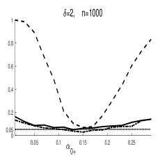
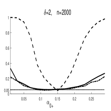
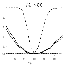
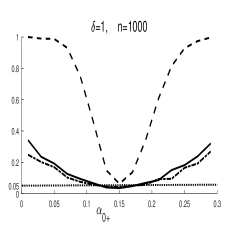
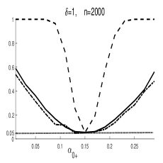
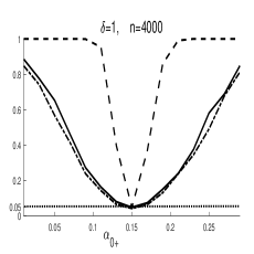
Figure 1: The power for the asymmetric test $\hat{S}_{1,r}$ (dotted line, - -), $\hat{S}_{2,r}^{(\tau_{1})}$ (solid line, -) and $\hat{S}_{2,r}^{(\tau_{2})}$ (solid and dotted line, -. ). Here, $r=1$, $\tau_{1}=0.05$, $\tau_{2}=0.1$, and $\eta_{t}\sim N(0,1)$.

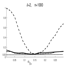
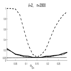
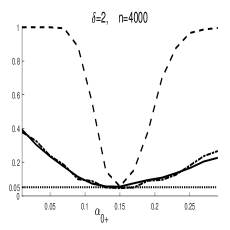
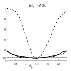
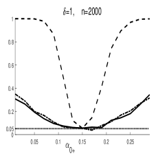
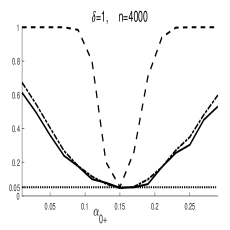
Figure 2: The power for the asymmetric test $\hat{S}_{1,r}$ (dotted line, - -), $\hat{S}_{2,r}^{(\tau_{1})}$ (solid line, -) and $\hat{S}_{2,r}^{(\tau_{2})}$ (solid and dotted line, -. ). Here, $r=1$, $\tau_{1}=0.05$, $\tau_{2}=0.1$, and $\eta_{t}\sim\mbox{st}_{5}$.

6 Applications

6.1 Stationary data

In this subsection, we re-analyze the daily log returns of two stock market indexes: the S&P 500 index and the Dow 30 index in Zheng et al. (2018). The data are observed on a daily basis from January 2, 2008 to June 30, 2016, with a sample size $n=2139$. Zheng et al. (2018) studied these two datasets by using the classical GARCH($1,1$) model, whose conditional quantile was estimated by the hybrid quantile estimator with the Guassian QMLE as its first step estimator. They found that the resulting method can produce better interval forecast than many existing ones. Since their GARCH($1,1$) model overlooks the often observed asymmetry effect in financial data, it is of interest to re-fit these two sequences by model (1.1).

Based on model (1.1) with $\delta=2$ and $1$, Table 6 gives the estimation results for both sequences. Here, we use the GQMLE $\tilde{\theta}_{n,r}$ with $r=2$ and $1$ in the first step estimation, and we consider the hybrid quantile estimators $\tilde{\theta}_{\tau n,r}$ with $\tau=0.05$ and $0.1$ in the second step estimation. From this table, the estimates of $\alpha_{0+}$ are always much smaller than those of $\alpha_{0-}$ in magnitude, indicating that there is a strong asymmetric effect for both sequences. To look for more evidence, we apply the asymmetry tests $\hat{S}_{1,r}$ and $\hat{S}_{2,r}^{(\tau)}$ to both sequences, and their corresponding p-values given in Table 6 confirm the asymmetric phenomenon. We also consider the strict stationarity test $\hat{T}_{r}$ for the testing problem (4.2) in Table 6, and its p-values show strong evidence that both time series are strictly stationary.

Next, we calculate the interval forecast of each sequence by the following expanding window procedure: first conduct the estimation using the data from January 2, 2008 to December 31, 2010 and compute the conditional quantile forecast for the next trading day, i.e., the forecast of $Q_{\tau}(\epsilon_{n+1}|\mathcal{F}_{n})$; then, advance the forecasting origin by one to include one more observation in the estimation subsample, and repeat the foregoing procedure until the end of the sample is reached.

Table 6: The estimation and testing results for the S&P 500 and Dow 30 returns

	$\delta=2$				$\delta=1$
	$r=2$		$r=1$		$r=2$		$r=1$
Panel A: S&P 500
$\omega$	4e-6 (9e-7)		2e-6 (4e-7)		7e-4 (1e-4)		3e-4 (5e-5)
$\alpha_{+}$	1e-7 (0.021)		4e-6 (0.011)		7e-6 (0.035)		1e-4 (0.017)
$\alpha_{-}$	0.261 (0.036)		0.156 (0.018)		0.302 (0.043)		0.205 (0.019)
$\beta$	0.848 (0.025)		0.850 (0.018)		0.835 (0.031)		0.862 (0.018)
$\omega_{\tau_{1}}$	-1e-5 (2e-5)		-1e-5 (2e-5)		-1e-3 (1e-3)		-9e-4 (1e-3)
$\alpha_{\tau_{1}+}$	-4e-7 (0.214)		-2e-5 (0.182)		-1e-5 (0.111)		-4e-4 (0.113)
$\alpha_{\tau_{1}-}$	-0.812 (0.357)		-0.872 (0.308)		-0.517 (0.111)		-0.476 (0.113)
$\beta_{\tau_{1}}$	-2.641 (0.004)		-4.689 (0.003)		-1.428 (0.172)		-2.002 (0.230)
$\omega_{\tau_{2}}$	-6e-6 (7e-6)		-5e-6 (8e-6)		-8e-4 (9e-4)		0.001 (9e-4)
$\alpha_{\tau_{2}+}$	-2e-7 (0.089)		-1e-5 (0.098)		-9e-6 (0.086)		-0.002 (0.082)
$\alpha_{\tau_{2}-}$	-0.431 (0.143)		-0.456 (0.160)		-0.388 (0.093)		-0.175 (0.088)
$\beta_{\tau_{2}}$	-1.403 (0.002)		-2.454 (0.002)		-1.072 (0.130)		-1.486 (0.154)
$\hat{T}_{r}$	1e-21		8e-14		7e-83		3e-51
$\hat{S}_{1,r}$	1e-13		1e-10		6e-15		7e-13
$\hat{S}_{2,r}^{(\tau_{1})}$	0.023		0.006		5e-6		4e-5
$\hat{S}_{2,r}^{(\tau_{2})}$	0.004		0.006		2e-5		0.030
Panel B: Dow 30
$\omega$	3e-6 (7e-7)		2e-6 (3e-7)		6e-4 (1e-4)		3e-4 (5e-5)
$\alpha_{+}$	4e-10 (0.019)		1e-8 (0.010)		2e-5 (0.029)		1e-5 (0.016)
$\alpha_{-}$	0.258 (0.035)		0.160 (0.018)		0.203 (0.037)		0.205(0.019)
$\beta$	0.852 (0.021)		0.852 (0.018)		0.839 (0.027)		0.863 (0.017)
$\omega_{\tau_{1}}$	-1e-5 (9e-6)		-8e-6 (9e-6)		-1e-3 (0.001)		-9e-4 (1e-3)
$\alpha_{\tau_{1}+}$	-1e-9 (0.156)		-5e-8 (0.158)		-4e-5 (0.114)		-2e-4 (0.122)
$\alpha_{\tau_{1}-}$	-0.784 (0.232)		-0.862 (0.218)		-0.501 (0.114)		-0.474 (0.119)
$\beta_{\tau_{1}}$	-2.590 (0.002)		-4.599 (0.002)		-1.447 (0.172)		-2.015 (0.230)
$\omega_{\tau_{2}}$	-5e-6 (6e-6)		-4e-6 (6e-6)		-8e-4 (9e-4)		-9e-4 (8e-4)
$\alpha_{\tau_{2}+}$	-7e-10 (0.095)		-3e-8 (0.099)		-3e-5 (0.090)		-5e-3 (0.088)
$\alpha_{\tau_{2}-}$	-0.427 (0.154)		-0.462 (0.166)		-0.377 (0.098)		-0.141 (0.095)
$\beta_{\tau_{2}}$	-1.411 (0.002)		-2.465 (0.002)		-1.087 (0.133)		-1.504 (0.159)
$\hat{T}_{r}$	5e-20		8e-14		1e-83		2e-51
$\hat{S}_{1,r}$	1e-15		2e-10		5e-15		7e-13
$\hat{S}_{2,r}^{(\tau_{1})}$	0.002		5e-4		7e-6		8e-5
$\hat{S}_{2,r}^{(\tau_{2})}$	0.008		0.007		1e-4		0.087

• ${\dagger}$ Note that $\tau_{1}=0.05$ and $\tau_{2}=0.1$.
  ${\ddagger}$ The standard deviations of all estimators are given in parentheses, and the p-values of all tests are given.

Moreover, we evaluate the forecasting performance of the aforementioned interval forecasts by using the following two measures:

(i) the minimum of the p-values of the two VaR backtests, the likelihood ratio test for correct conditional converge (CC) in Christoffersen (1998) and the dynamic quantile (DQ) test in Engle and Manganelli (2004);

(ii) the empirical coverage error is defined as the proportion of observations that exceed the corresponding VaR forecast minus the corresponding nominal level $\tau$.

The reason for selecting the smaller of the two p-values is that the CC and DQ tests have different null hypotheses and hence are complementary to each other. Note that a larger p-value of either CC or DQ test gives a stronger evidence of good interval forecasts.

Table 7: Minimum p-values of two VaR backtests and empirical coverage errors for the S&P 500 and Dow 30 returns at the lower (L) (or upper (U)) 0.01th, 0.025th, and 0.05th conditional quantiles

		Minimum p-value of VaR backtests								Empirical coverage error
		$\delta=2$					$\delta=1$			$\delta=2$					$\delta=1$
		$r=2$								$r=2$
	$\tau$	$\alpha_{0+}=\alpha_{0-}$		$\alpha_{0+}\not=\alpha_{0-}$	$r=1$		$r=2$	$r=1$		$\alpha_{0+}=\alpha_{0-}$		$\alpha_{0+}\not=\alpha_{0-}$	$r=1$		$r=2$	$r=1$
S&P 500	L1.0	0.000		0.0000	0.0000		0.0000	0.0000		-0.0002		-0.0069	-0.0069		-0.0088	-0.0076
	L2.5	0.001		0.0000	0.0000		0.0000	0.0000		-0.0048		-0.0226	-0.0195		-0.0183	-0.0183
	L5.0	0.017		0.0000	0.0000		0.0000	0.0000		-0.0090		-0.0427	-0.0378		-0.0323	-0.0255
	U5.0	0.245		0.6996	0.6304		0.4846	0.2401		0.0054		0.0041	0.0023		0.0047	0.0011
	U2.5	0.356		0.7142	0.7616		0.1476	0.2807		0.0030		0.0030	0.0011		0.0060	0.0048
	U1.0	0.275		0.8504	0.2956		0.8213	0.6206		0.0008		0.0002	-0.0028		0.0008	0.0020
Dow 30	L1.0	0.063		0.0000	0.0000		0.000	0.0000		-0.0014		-0.0076	-0.0027		-0.0088	-0.0076
	L2.5	0.000		0.0000	0.0000		0.0000	0.0000		-0.0054		-0.0249	-0.0201		-0.0213	-0.213
	L5.0	0.000		0.0000	0.0000		0.000	0.0000		-0.0072		-0.0433	-0.0420		-0.0329	-0.0286
	U5.0	0.273		0.1678	0.2304		0.1842	0.2798		0.0084		0.0072	0.0035		0.0060	0.0023
	U2.5	0.568		0.3493	0.3723		0.6350	0.3723		0.0011		0.0024	0.0005		0.0011	0.0001
	U1.0	0.418		0.8256	0.8256		0.1296	0.0002		-0.0028		-0.0004	-0.0004		0.0045	0.0020

• ${\dagger}$ Among the models with p-values $>5\%$, the largest p-value and the smallest empirical coverage error (in absolute value) are in boldface.

Based on model (1.1) with $\delta=2$ and 1, Table 7 reports the results of two measures at the lower (L) (or upper(U)) 0.01th, 0.025th and 0.05th conditional quantiles. Here, the GQMLE $\tilde{\theta}_{n,r}$ with $r=2$ and $1$ is used in the first step estimation. As a comparison, the results for the benchmark method (i.e., $\delta=2,r=2$ and $\alpha_{0+}=\alpha_{0-}$) in Zheng et al. (2018) are also included in Table 7. It can be seen that all methods have a poor performance for the lower conditional quantiles, while our proposed methods, based on the asymmetric model (1.1) together with the hybrid quantile estimation, have a significantly better interval forecasting performance for the upper conditional quantiles than the benchmark method in Zheng et al. (2018). The poor performance of the lower conditional quantiles from our method may be because our GQMLE $\tilde{\theta}_{n,r}$ does not account for the asymmetry of $\eta_{t}$. We may expect to improve our forecasting performance particularly for the lower conditional quantiles by using a skewed distribution of $\eta_{t}$ to form our first estimation, and we leave this desired direction for future study. In terms of the minimum of the p-values of the two VaR backtests, our proposed methods with $\delta=2$ are better than those with $\delta=1$ in four out of six cases, while the choice of $r$ seems irrelevant to the forecasting performance. In terms of the empirical coverage error, our proposed methods with $\delta=2$ (or $r=1$) are better than those with $\delta=1$ (or $r=2$) in general. Overall, our method with $\delta=2$, $r=2$ and $\alpha_{0+}\not=\alpha_{0-}$ has the best interval forecasting performance for both data.

6.2 Non-stationary data

In this subsection, we re-visit three daily stock return data sequences of Community Bankers Trust (BTC), China MediaExpress (CCME) and Monarch Community Bancorp (MCBF) in Francq and Zakoïan (2012, 2013a). These three sequences are shown to be non-stationary in Francq and Zakoïan (2012), while their conditional quantile estimators have not been investigated. Motivated by this, we study their conditional quantiles by our hybrid quantile estimation method. To compute our hybrid quantile estimator, we choose the GQMLE $\tilde{\theta}_{n,r}$ with $r=1$ in the first estimation step. Here, we do not consider the GQMLE $\tilde{\theta}_{n,r}$ with $r=2$, since Li et al. (2018) demonstrated the innovations of the fitted GARCH($1,1$) model for each sequence only have a finite second moment but not an infinite fourth moment. In the second step of quantile estimation, we consider the hybrid quantile estimators $\hat{\theta}_{\tau n,1}$ at levels $\tau=0.05$ and $0.1$. Table 8 reports the results of $\tilde{\theta}_{n,1}$ and $\hat{\theta}_{\tau n,1}$ for each sequence, together with the results of $\hat{T}_{1}$ for the testing problem (4.2). From the results of $\hat{T}_{1}$, we can reach the same conclusion as in Francq and Zakoïan (2012) that all three data are non-stationary, and hence the estimates for the drift term $\omega$ or $\omega_{\tau}$ may not be consistent. Meanwhile, Table 8 reports the results of $\hat{S}_{1,1}$, $\hat{S}_{2,1}^{(0.05)}$ and $\hat{S}_{2,1}^{(0.1)}$ for the testing problem (4.5). It is interesting to observe that the global asymmetry test $\hat{S}_{1,1}$ as the one in Francq and Zakoïan (2013a) indicates that all three datasets do not have the asymmetric effect, while the local asymmetry tests $\hat{S}_{2,1}^{(0.05)}$ and $\hat{S}_{2,1}^{(0.1)}$ detect some strong asymmetric effects in model (1.1) with $\delta=2$ or $1$ for the CCME and MCBF data. Although none of the considered tests can find the asymmetric evidence for the BTC data, we think the examined BTC data still have the asymmetric effect, since our forecasting comparison below indicates that the asymmetric PGARCH model can perform better than its symmetric counterpart.

Table 8: The estimation and testing results for the BTC, CCME and MCBF returns

	Panel A: BTC				Panel B: CCME				Panel C: MCBF
	$\delta=2$		$\delta=1$		$\delta=2$		$\delta=1$		$\delta=2$		$\delta=1$
$\omega$	8e-7 (7e-8)		1e-4 (1e-4)		2e-8 (2e-8)		1e-4 (2e-5)		8e-6 (4e-6)		8e-4 (3e-4)
$\alpha_{+}$	0.089 (0.035)		0.130 (0.040)		0.107 (0.047)		0.148 (0.048)		0.033 (0.016)		0.078 (0.003)
$\alpha_{-}$	0.119 (0.038)		0.172 (0.041)		0.125 (0.063)		0.161 (0.056)		0.029 (0.014)		0.078 (0.028)
$\beta$	0.840 (0.031)		0.854 (0.027)		0.838 (0.043)		0.860 (0.033)		0.931 (0.019)		0.902 (0.024)
$\omega_{\tau_{1}}$	-5e-7 (1e-6)		-9e-4 (4e-4)		-1e-9 (6e-7)		-1e-7 (3e-4)		-2e-7 (1e-4)		-9e-4 (0.005)
$\alpha_{\tau_{1}+}$	-0.448 (0.229)		-0.320 (0.211)		-0.639 (0.421)		-0.498 (0.295)		-1.515 (0.221)		-0.479 (0.346)
$\alpha_{\tau_{1}-}$	-0.661 (0.215)		-0.423 (0.182)		-1.879 (0.504)		-0.846 (0.298)		-1e-4 (0.086)		-0.009 (0.144)
$\beta_{\tau_{1}}$	-4.660 (1e-4)		-2.097 (0.060)		-3.190 (1e-4)		-1.772 (0.032)		-4.625 (0.009)		-2.037 (0.263)
$\omega_{\tau_{2}}$	-8e-8 (7e-7)		-2e-7 (3e-4)		-4e-13 (2e-7)		-3e-8 (2e-4)		-1e-8 (9e-5)		-1e-4 (0.003)
$\alpha_{\tau_{2}+}$	-0.348 (0.211)		-0.153 (0.140)		-0.364 (0.268)		-0.404 (0.191)		-0.596 (0.229)		-0.314 (0.173)
$\alpha_{\tau_{2}-}$	-0.198 (0.178)		-0.113 (0.106)		-0.741 (0.267)		-0.792 (0.182)		-2e-5 (0.088)		0.005 (0.095)
$\beta_{\tau_{2}}$	-2.232 (1e-4)		-1.522 (0.004)		-1.450 (1e-4)		-0.948 (0.021)		-2.438 (0.008)		-1.534 (0.151)
$\hat{T}_{r}$	0.397		0.966		0.145		0.577		0.894		0.143
$\hat{S}_{1,r}$	0.222		0.208		0.409		0.424		0.429		0.499
$\hat{S}_{2,r}^{(\tau_{1})}$	0.257		0.359		0.032		0.210		1e-4		0.063
$\hat{S}_{2,r}^{(\tau_{2})}$	0.298		0.411		0.164		0.076		0.008		0.035

• ${\dagger}$ Note that $r=1$, $\tau_{1}=0.05$ and $\tau_{2}=0.1$.
  ${\ddagger}$ The standard deviations of all estimators are given in parentheses, and the p-values of all tests are given.

Table 9: Minimum p-values of two VaR backtests and empirical coverage errors for the BTC, CCME and MCBF returns at the lower (L) (or upper (U)) 0.01th, 0.025th, and 0.05th conditional quantiles

		Minimum p-value of VaR backtests						Empirical coverage error
		$\delta=2$						$\delta=2$
	$\tau$	$\alpha_{0+}=\alpha_{0-}$		$\alpha_{0+}\not=\alpha_{0-}$		$\delta=1$		$\alpha_{0+}=\alpha_{0-}$		$\alpha_{0+}\not=\alpha_{0-}$		$\delta=1$
BTC	L1.0	0.0025		0.3999		0.9329		-0.0100		-0.0056		-0.0012
	L2.5	0.0000		0.0025		0.3335		-0.0250		-0.0206		-0.0096
	L5.0	0.0000		0.0000		0.0031		-0.0302		-0.0478		-0.0302
	U5.0	0.0299		0.1265		0.0182		0.0500		0.0170		0.0192
	U2.5	0.0003		0.6372		0.0877		0.0228		0.0052		0.0008
	U1.0	0.1296		0.8130		0.2569		0.0038		-0.0010		-0.0032
CCME	L1.0	0.0301		0.9574		0.9574		-0.0100		-0.0015		-0.0015
	L2.5	0.0006		0.0001		0.0000		-0.0250		-0.0165		-0.0165
	L5.0	0.0000		0.0000		0.0000		-0.0500		-0.0415		-0.0415
	U5.0	0.0002		0.0000		0.0080		0.0457		0.0457		0.0372
	U2.5	0.0433		0.0006		0.0006		0.0207		0.0250		0.0250
	U1.0	0.6077		0.6077		0.0301		0.0057		0.0057		0.0100
MCBF	L1.0	0.0031		0.0031		0.0031		-0.0100		-0.0100		-0.0100
	L2.5	0.0038		0.2131		0.4400		-0.0204		-0.0112		0.0050
	L5.0	0.0023		0.1220		0.1682		-0.0316		-0.0177		-0.0131
	U5.0	0.0067		0.0023		0.0001		0.0200		0.0316		-0.0030
	U2.5	0.0005		0.7622		0.0001		0.0227		0.0020		-0.0188
	U1.0	0.0031		0.0000		0.7747		0.0100		0.0008		0.0031

• ${\dagger}$ Among the models with p-values $>5\%$, the largest p-value and the smallest empirical coverage error (in absolute value) are in boldface.

Next, we compute the interval forecasts for each sequence by using the same procedure as in Subsection 6.1, except that the first interval forecast is calculated based on the first half of sample. Again, we follow the measurements as in Subsection 6.1 to evaluate the interval forecasting performance of our methods, based on model (1.1) with the hybrid quantile estimators. Table 9 reports the corresponding results for all three datasets. As a comparison, the forecasting performance of the benchmark GARCH($1,1$) model (i.e., $\delta=2$ and $\alpha_{0+}=\alpha_{0-}$) estimated by the Laplacian QMLE $\tilde{\theta}_{n,1}$ is also given in Table 9. It can be seen that, in terms of minimum p-values of two VaR backtests, model (1.1) with $\delta=1$ (or $\delta=2$ and $\alpha_{0+}\not=\alpha_{0-}$) can provide us with a good interval forecast in 6 cases, while the benchmark GARCH($1,1$) model can only do this in one case. Similar conclusions can be obtained in terms of empirical coverage error. Particularly, our forecasting results indicate that the BTC data have the asymmetric effect, which, however, has not been detected by our considered tests in Table 8. Note that there are 7 cases (most of them are for the CCME data) in which none of the methods can deliver a satisfactory interval forecast, and these cases may require some new methods for their interval forecast.

7 Conclusion

In this paper, the hybrid quantile estimators are proposed for the asymmetric PGARCH models via the transformation $T(x)=|x|^{\delta}\mbox{sgn}(x)$. Asymptotic normality for the quantile estimators is established under both stationarity and non-stationarity. As a result, tests for strict stationarity and asymmetry are obtained. It is hoped these results will add to the tool kits of time series analysis.

Appendix: Proofs

To facilitate our proofs, we first introduce some notations. Let $\Theta_{0}=\{\theta\in\Theta:\beta<e^{\gamma_{0}}\}$ and $\Theta_{p}=\{\theta\in\mathcal{R}_{+}^{4}:\beta<\|1/a_{0}(\eta_{t})\|_{p}^{-1}\}$. Define four $[0,\infty]$-valued processes

$$v_{t}(\vartheta)=\sum_{j=1}^{\infty}\frac{\{\alpha_{+}(\eta_{t-j}^{+})^{\delta}+\alpha_{-}(-\eta_{t-j}^{-})^{\delta}\}}{a_{0}(\eta_{t-j})}\prod_{k=1}^{j-1}\frac{\beta}{a_{0}(\eta_{t-k})},$$

$$d_{t}^{\alpha_{+}}(\vartheta)=\sum_{j=1}^{\infty}\frac{(\eta_{t-j}^{+})^{\delta}}{a_{0}(\eta_{t-j})}\prod_{k=1}^{j-1}\frac{\beta}{a_{0}(\eta_{t-k})},\ \ \ d_{t}^{\alpha_{-}}(\vartheta)=\sum_{j=1}^{\infty}\frac{(-\eta_{t-j}^{-})^{\delta}}{a_{0}(\eta_{t-j})}\prod_{k=1}^{j-1}\frac{\beta}{a_{0}(\eta_{t-k})},$$

$$d_{t}^{\beta}(\vartheta)=\sum_{j=2}^{\infty}\frac{(j-1)\{\alpha_{+}(\eta_{t-j}^{+})^{\delta}+\alpha_{-}(-\eta_{t-j}^{-})^{\delta}\}}{\beta a_{0}(\eta_{t-j})}\prod_{k=1}^{j-1}\frac{\beta}{a_{0}(\eta_{t-k})}$$

with the convention $\prod_{k=1}^{j-1}=1$ when $j\leq 1$. As shown in Francq and Zakoïan (2013a), $v_{t}(\vartheta)$, $1/v_{t}(\vartheta)$, $d_{t}^{\alpha_{+}}(\vartheta)$, $d_{t}^{\alpha_{-}}(\vartheta)$ and $d_{t}^{\beta}(\vartheta)$ have moments of any order.

Second, we give six technical lemmas. Lemmas .1-.2 from Francq and Zakoïan (2013a) show that, after being normalized by $h_{t}$, the nonstationary process $\sigma_{t}^{\delta}(\theta)$ and its first derivatives can be well approximated by some stationary processes. Lemma .3 gives the asymptotic properties of the GQMLE $\tilde{\theta}_{n,r}$, and its proof is similar to that of Theorem 3.1 in Francq and Zakoïan (2013a). Lemma .4 proves the consistency of $\tilde{\vartheta}_{n,r}$ for $\gamma_{0}\geq 0$. Lemmas .5-.6 are used to for the proof of Theorem 3.1.

Lemma .1.

Suppose that Assumption 3.1(ii) holds.

(i) When $\gamma_{0}>0$, for any $\theta\in\Theta_{0}$, the process $v_{t}(\vartheta)$ is stationary and ergodic. Moreover, for any compact set $\Theta_{0}^{*}\subset\Theta_{0}$,

$$\sup_{\theta\in\Theta_{0}^{*}}\left|\frac{\sigma_{t}^{\delta}(\theta)}{h_{t}}-v_{t}(\vartheta)\right|\rightarrow 0\mbox{ a.s. as $t\rightarrow\infty$},$$

and

$$\sup_{\theta\in\Theta_{0}^{*}}\left|\frac{h_{t}}{\sigma_{t}^{\delta}(\theta)}-\frac{1}{v_{t}(\vartheta)}\right|\rightarrow 0\mbox{ a.s. as $t\rightarrow\infty$}.$$

Finally, for any $\theta\not\in\Theta_{0}$, it holds that $\sigma_{t}^{\delta}(\theta)/h_{t}\to\infty$ as $t\to\infty$.

(ii) When $\gamma_{0}=0$, for any $\theta\in\Theta_{p}$ with $p\geq 1$, the process $v_{t}(\vartheta)$ is stationary and ergodic. Moreover, for any compact set $\Theta_{p}^{*}\subset\Theta_{p}$,

$$\sup_{\theta\in\Theta_{p}^{*}}\left|\frac{\sigma_{t}^{\delta}(\theta)}{h_{t}}-v_{t}(\vartheta)\right|\rightarrow 0\mbox{ in $L^{p}$ as $t\rightarrow\infty$},$$

and

$$\sup_{\theta\in\Theta_{p}^{*}}\left|\frac{h_{t}}{\sigma_{t}^{\delta}(\theta)}-\frac{1}{v_{t}(\vartheta)}\right|\rightarrow 0\mbox{ in $L^{p}$ as $t\rightarrow\infty$}.$$

Lemma .2.

Suppose that Assumption 3.1(ii) holds.

(i) When $\gamma_{0}>0$, for any $\theta\in\Theta_{0}$, the processes $d_{t}^{\alpha_{+}}(\vartheta)$, $d_{t}^{\alpha_{-}}(\vartheta)$, and $d_{t}^{\beta}(\vartheta)$ are stationary and ergodic. Moreover, for any compact set $\Theta_{0}^{*}\subset\Theta_{0}$,

$$\sup_{\theta\in\Theta_{0}^{*}}\left\|\frac{1}{h_{t}}\frac{\partial\sigma_{t}^{\delta}(\theta)}{\partial\vartheta}-d_{t}(\vartheta)\right\|\rightarrow 0\mbox{ a.s. as $t\rightarrow\infty$},$$

where

$$d_{t}(\vartheta)=(d_{t}^{\alpha_{+}}(\vartheta),d_{t}^{\alpha_{-}}(\vartheta),d_{t}^{\beta}(\vartheta))^{\prime}.$$ (.1)

(ii) When $\gamma_{0}=0$, for any $\theta\in\Theta_{p}$ with $p\geq 1$, the processes $d_{t}^{\alpha_{+}}(\vartheta)$, $d_{t}^{\alpha_{-}}(\vartheta)$, and $d_{t}^{\beta}(\vartheta)$ are stationary and ergodic. Moreover, for any compact set $\Theta_{p}^{*}\subset\Theta_{p}$,

$$\sup_{\theta\in\Theta_{p}^{*}}\left\|\frac{1}{h_{t}}\frac{\partial\sigma_{t}^{\delta}(\theta)}{\partial\vartheta}-d_{t}(\vartheta)\right\|\rightarrow 0\mbox{ in}\ L^{p}\ \mbox{as}\ t\rightarrow\infty.$$

Lemma .3.

Suppose that Assumption 3.1 holds and $E|\eta_{t}|^{2r}<\infty$.

(i) When $\gamma_{0}<0$, and $\beta<1$ for all $\theta\in\Theta$, then $\tilde{\theta}_{n,r}\rightarrow\theta_{0}$ a.s. as $n\rightarrow\infty$, and

$$\sqrt{n}(\tilde{\theta}_{n,r}-\theta_{0}) =-\frac{\delta J^{-1}}{r\sqrt{n}}\sum_{t=1}^{n}[1-|\eta_{t}|^{r}]\frac{1}{h_{t}}\frac{\partial h_{t}(\theta_{0})}{\partial\theta}+o_{p}(1)$$

$$\rightarrow_{d}N(0,\kappa_{2r}\delta^{2}J^{-1})\mbox{ as }n\to\infty.$$ (.2)

(ii) When $\gamma_{0}>0$, and $P(\eta_{t}=0)=0$, then $\tilde{\vartheta}_{n,r}\rightarrow\vartheta_{0}$ a.s. as $n\rightarrow\infty$, and

$$\sqrt{n}(\tilde{\vartheta}_{n,r}-\vartheta_{0}) =-\frac{\delta J_{\vartheta}^{-1}}{r\sqrt{n}}\sum_{t=1}^{n}[1-|\eta_{t}|^{r}]\frac{1}{h_{t}}\frac{\partial\sigma_{t}^{\delta}(\theta_{0})}{\partial\vartheta}+o_{p}(1)$$

$$\rightarrow_{d}N(0,\kappa_{2r}\delta^{2}J_{\vartheta}^{-1})\mbox{ as }n\to\infty.$$ (.3)

(iii) When $\gamma_{0}=0$, $P(\eta_{t}=0)=0$, and $\beta<\|1/a_{0}(\eta_{t})\|_{p}^{-1}$ for any $\theta\in\Theta$ and some $p>1$, then $\tilde{\vartheta}_{n,r}\rightarrow\vartheta_{0}$ in probability as $n\rightarrow\infty$, and (.3) holds provided that Assumption 3.3 is satisfied.

Lemma .4.

Suppose that Assumptions 3.1-3.2 hold and $E|\eta_{t}|^{2r}<\infty$.

(i) When $\gamma_{0}>0$, and $P(\eta_{t}=0)=0$, then $\hat{\vartheta}_{\tau n,r}\rightarrow\vartheta_{\tau 0}$ in probability as $n\rightarrow\infty$.

(ii) When $\gamma_{0}=0$, $P(\eta_{t}=0)=0$, and $\beta<\|1/a_{0}(\eta_{t})\|_{p}^{-1}$ for any $\theta\in\Theta$ and some $p>1$, then $\hat{\vartheta}_{\tau n,r}\rightarrow\vartheta_{\tau 0}$ in probability as $n\rightarrow\infty$.

Proof.

We only show the proof of (i), and the proof of (ii) is similar.

First, by (2), it is straightforward that $(\hat{\omega}_{\tau n,r},\hat{\vartheta}_{\tau n,r}^{\prime})^{\prime}=\operatornamewithlimits{argmin}_{\theta_{\tau}\in\Theta_{\tau}}Q_{n}(\theta_{\tau})$, where $Q_{n}(\theta_{\tau})=\frac{1}{n}\sum_{t=1}^{n}[l_{t,\rho}(\theta_{\tau})-l_{t,\rho}^{{\dagger}}]$ with $l_{t,\rho}^{{\dagger}}=\rho_{\tau}\big{(}\frac{y_{t}}{\sigma_{t}^{\delta}(\tilde{\theta}_{n,r})}-b_{\tau}\big{)}$. By using the identity

$$\rho_{\tau}(x-y)-\rho_{\tau}(x)=-y\psi_{\tau}(x)+\int_{0}^{y}\left[\mbox{I}(x\leq s)-\mbox{I}(x\leq 0)\right]ds$$

with $\psi_{\tau}(x)=\tau-\mbox{I}(x<0)$, it follows that

$$Q_{n}(\theta_{\tau}) =-\frac{1}{n}\sum_{t=1}^{n}\left[\frac{\theta_{\tau}^{\prime}\tilde{z}_{t}}{\sigma_{t}^{\delta}(\tilde{\theta}_{n,r})}-b_{\tau}\right]\psi_{\tau}\left(\frac{y_{t}}{\sigma_{t}^{\delta}(\tilde{\theta}_{n,r})}-b_{\tau}\right)$$

$$\quad\quad+\frac{1}{n}\sum_{t=1}^{n}\int_{0}^{\frac{\theta_{\tau}^{\prime}\tilde{z}_{t}}{\sigma_{t}^{\delta}(\tilde{\theta}_{n,r})}-b_{\tau}}\mbox{I}\left(\frac{y_{t}}{\sigma_{t}^{\delta}(\tilde{\theta}_{n,r})}\leq s+b_{\tau}\right)-\mbox{I}\left(\frac{y_{t}}{\sigma_{t}^{\delta}(\tilde{\theta}_{n,r})}\leq b_{\tau}\right)ds$$

$$\equiv-I_{11}(\theta_{\tau})+I_{12}(\theta_{\tau}).$$ (.4)

Next, we consider $I_{11}(\theta_{\tau})$. By Proposition 2.1 in Francq and Zakoïan (2013a), $h_{t}\to\infty$ as $t\to\infty$, and hence

$$\left|\frac{h_{t-1}}{h_{t}}-\frac{1}{a_{0}(\eta_{t-1})}\right|=\left|\frac{-\omega_{0}}{a_{0}(\eta_{t-1})h_{t}}\right|\to 0\mbox{ as }t\to\infty.$$ (.5)

By Lemma .1(i), it follows that

$$\sup_{\theta\in\Theta_{0}^{*}}\left|\frac{\sigma_{t-1}^{\delta}(\theta)}{h_{t}}-\frac{v_{t-1}(\vartheta)}{a_{0}(\eta_{t-1})}\right|\rightarrow 0\mbox{ a.s. as $t\rightarrow\infty$}.$$ (.6)

Define $Z_{t}(\theta)=(1,(\epsilon_{t-1}^{+})^{\delta},(-\epsilon_{t-1}^{-})^{\delta},\sigma^{\delta}_{t-1}(\theta))^{\prime}$ and $\varsigma_{t}(\vartheta)=\big{(}0,\frac{(\eta_{t-1}^{+})^{\delta}}{a_{0}(\eta_{t-1})},\frac{(-\eta_{t-1}^{-})^{\delta}}{a_{0}(\eta_{t-1})},\frac{v_{t-1}(\vartheta)}{a_{0}(\eta_{t-1})}\big{)}^{\prime}$. Since $(\epsilon_{t-1}^{+})^{\delta}/h_{t-1}=(\eta_{t-1}^{+})^{\delta}$ and $(-\epsilon_{t-1}^{-})^{\delta}/h_{t-1}=(-\eta_{t-1}^{-})^{\delta}$, by (.5)-(.6) we have

$$\sup_{\theta\in\Theta_{0}^{*}}\left\|\frac{Z_{t}(\theta)}{h_{t}}-\varsigma_{t}(\vartheta)\right\|\rightarrow 0\mbox{ a.s. as $t\rightarrow\infty$}.$$ (.7)

Note that $\tilde{z}_{t}=Z_{t}(\tilde{\theta}_{n,r})$ and $y_{t}=T(\eta_{t})h_{t}$. Then, it is not difficult to have

$$I_{11}(\theta_{\tau}) =\frac{1}{n}\sum_{t=1}^{n}\left[\frac{\theta_{\tau}^{\prime}\tilde{z}_{t}/h_{t}}{\sigma_{t}^{\delta}(\tilde{\theta}_{n,r})/h_{t}}-b_{\tau}\right]\psi_{\tau}\left(\frac{T(\eta_{t})}{\sigma_{t}^{\delta}(\tilde{\theta}_{n,r})/h_{t}}-b_{\tau}\right)$$

$$=\frac{1}{n}\sum_{t=1}^{n}\left[\frac{\theta_{\tau}^{\prime}\varsigma_{t}(\tilde{\vartheta}_{n,r})}{v_{t}(\tilde{\vartheta}_{n,r})}-b_{\tau}\right]\psi_{\tau}\left(\frac{T(\eta_{t})}{\sigma_{t}^{\delta}(\tilde{\theta}_{n,r})/h_{t}}-b_{\tau}\right)+o_{p}(1)$$

$$=\frac{1}{n}\sum_{t=1}^{n}\left[\frac{\theta_{\tau}^{\prime}\varsigma_{t}(\vartheta_{0})}{v_{t}(\vartheta_{0})}-b_{\tau}\right]\psi_{\tau}\left(\frac{T(\eta_{t})}{\sigma_{t}^{\delta}(\tilde{\theta}_{n,r})/h_{t}}-b_{\tau}\right)+o_{p}(1),$$ (.8)

where the second equality holds by Lemma .1(i), (.7) and the boundedness of $\psi_{\tau}(\cdot)$, and the last equality holds by Taylor’s expansion, Lemma .3(ii), and the fact that

$$\sup_{\theta\in\Theta_{0}}\left|\frac{1}{n}\sum_{t=1}^{n}\frac{\partial}{\partial\vartheta}\left(\frac{\varsigma_{t}(\vartheta)}{v_{t}(\vartheta)}\right)\right|=O_{p}(1).$$

Furthermore, by the double expectation, Lemma .1(i), Assumption 3.2, and standard arguments for tightness, we can prove

$$\sup_{\theta\in\Theta}\left|\frac{1}{n}\sum_{t=1}^{n}\left[\frac{\theta_{\tau}^{\prime}\varsigma_{t}(\vartheta_{0})}{v_{t}(\vartheta_{0})}-b_{\tau}\right]\left[\psi_{\tau}\left(\frac{T(\eta_{t})}{\sigma_{t}^{\delta}(\theta)/h_{t}}-b_{\tau}\right)-\psi_{\tau}\left(\frac{T(\eta_{t})}{v_{t}(\vartheta)}-b_{\tau}\right)\right]\right|$$

$$\quad=o_{p}(1).$$ (.9)

Hence, by (Proof.) and (Proof.), it follows that

$$I_{11}(\theta_{\tau}) =\frac{1}{n}\sum_{t=1}^{n}\left[\frac{\theta_{\tau}^{\prime}\varsigma_{t}(\vartheta_{0})}{v_{t}(\vartheta_{0})}-b_{\tau}\right]\psi_{\tau}\left(\frac{T(\eta_{t})}{v_{t}(\tilde{\vartheta}_{n,r})}-b_{\tau}\right)+o_{p}(1)$$

$$=E\left\{\left[\frac{\theta_{\tau}^{\prime}\varsigma_{t}(\vartheta_{0})}{v_{t}(\vartheta_{0})}-b_{\tau}\right]\psi_{\tau}\left(\frac{T(\eta_{t})}{v_{t}(\tilde{\vartheta}_{n,r})}-b_{\tau}\right)\right\}+o_{p}(1)$$

$$=E\left\{\left[\frac{\theta_{\tau}^{\prime}\varsigma_{t}(\vartheta_{0})}{v_{t}(\vartheta_{0})}-b_{\tau}\right]\psi_{\tau}\left(\frac{T(\eta_{t})}{v_{t}(\vartheta_{0})}-b_{\tau}\right)\right\}+o_{p}(1)$$

$$=E\left\{\left[\vartheta_{\tau}^{\prime}\xi_{t}-b_{\tau}\right]\psi_{\tau}\left(T(\eta_{t})-b_{\tau}\right)\right\}+o_{p}(1)$$

$$=o_{p}(1),$$ (.10)

where the second equality holds by the uniform ergodic theorem, the third equality holds by the dominated convergence theorem and Lemma .3(ii), the fourth equality holds since $v_{t}(\vartheta_{0})=1$ and $\varsigma_{t}(\vartheta_{0})=(0,\xi_{t})$, and the last equality holds by the double expectation and the fact that the $\tau$th quantile of $T(\eta_{t})$ is $b_{\tau}$.

Third, we consider $I_{12}(\theta_{\tau})$. As for (Proof.), we can show

$$I_{12}(\theta_{\tau}) =E\left\{\int_{0}^{\vartheta_{\tau}^{\prime}\xi_{t}-b_{\tau}}\mbox{I}\left(T(\eta_{t})\leq s+b_{\tau}\right)-\mbox{I}\left(T(\eta_{t})\leq b_{\tau}\right)ds\right\}+o_{p}(1)$$

$$=E\left\{\int_{0}^{\vartheta_{\tau}^{\prime}\xi_{t}-\vartheta_{\tau 0}^{\prime}\xi_{t}}[f(\breve{\vartheta}_{\tau})]s\,ds\right\}+o_{p}(1)$$

$$\equiv H(\vartheta_{\tau})+o_{p}(1),$$ (.11)

where $\breve{\vartheta}_{\tau}$ lies between $s+b_{\tau}$ and $b_{\tau}$, and the second equality holds by the double expectation, Taylor’s expansion, and the fact that $b_{\tau}=\vartheta_{\tau 0}^{\prime}\xi_{t}$.

Note that $|\breve{\vartheta}_{\tau}|\leq|b_{\tau}|+|(\vartheta_{\tau}-\vartheta_{\tau 0})^{\prime}\xi_{t}|\leq C_{0}$ for some constant $C_{0}>0$. By (Proof.), (Proof.) and (Proof.), we have that $Q_{n}(\theta_{\tau})=H(\vartheta_{\tau})+o_{p}(1)$, where

$$H(\vartheta_{\tau})\geq(\vartheta_{\tau}-\vartheta_{\tau 0})^{\prime}E\left\{\frac{[\inf_{|x|\leq C_{0}}f(x)]}{2}\xi_{t}\xi_{t}^{\prime}\right\}(\vartheta_{\tau}-\vartheta_{\tau 0}),$$

and the equality holds if and only if $\vartheta_{\tau}=\vartheta_{\tau 0}$. Hence, the proof of (i) is completed by standard arguments, invoking the compactness of $\Theta_{\tau}$. ∎

Write $\tilde{z}_{t}=(1,\tilde{z}_{t,\vartheta}^{\prime})^{\prime}$, where $\tilde{z}_{t,\vartheta}=((\epsilon_{t-1}^{+})^{\delta},(-\epsilon_{t-1}^{-})^{\delta},\sigma^{\delta}_{t-1}(\tilde{\theta}_{n,r}))^{\prime}$. Define $\bar{z}_{t}=(1,\bar{z}_{t,\vartheta}^{\prime})^{\prime}$, where $\bar{z}_{t,\vartheta}=((\epsilon_{t-1}^{+})^{\delta},(-\epsilon_{t-1}^{-})^{\delta},\sigma^{\delta}_{t-1}(\theta_{0}))^{\prime}.$

Lemma .5.

Suppose that Assumptions 3.1-3.2 hold and $E|\eta_{t}|^{2r}<\infty$.

(i) If $\gamma_{0}>0$, and $P(\eta_{t}=0)=0$, then

$$I_{2}=o_{p}(1),\,\,\,\,\,\,I_{3}=-f(b_{\tau})b_{\tau}\Gamma_{\vartheta}[\sqrt{n}(\tilde{\vartheta}_{n,r}-\vartheta_{0})]+o_{p}(1),$$ (.12)

$$\mbox{ and }I_{4}=[-f(b_{\tau})\Omega_{\vartheta}+o_{p}(1)][\sqrt{n}(\hat{\vartheta}_{\tau n,r}-\vartheta_{\tau 0})]+o_{p}(1),$$ (.13)

where

$$I_{2} =\frac{1}{\sqrt{n}}\sum_{t=1}^{n}\psi_{\tau}\left(y_{t}-\hat{\theta}_{\tau n,r}^{\prime}\tilde{z}_{t}\right)\left[\frac{\tilde{z}_{t,\vartheta}}{\sigma^{\delta}_{t}(\tilde{\theta}_{n,r})}-\frac{\bar{z}_{t,\vartheta}}{\sigma^{\delta}_{t}(\theta_{0})}\right],$$

$$I_{3} =\frac{1}{\sqrt{n}}\sum_{t=1}^{n}\left[\psi_{\tau}\left(y_{t}-\hat{\theta}_{\tau n,r}^{\prime}\tilde{z}_{t}\right)-\psi_{\tau}\left(y_{t}-\hat{\theta}_{\tau n,r}^{\prime}\bar{z}_{t}\right)\right]\frac{\bar{z}_{t,\vartheta}}{\sigma^{\delta}_{t}(\theta_{0})},$$

$$I_{4} =\frac{1}{\sqrt{n}}\sum_{t=1}^{n}\left[\psi_{\tau}\left(y_{t}-\hat{\theta}_{\tau n,r}^{\prime}\bar{z}_{t}\right)-\psi_{\tau}\left(y_{t}-\theta_{\tau 0}^{\prime}\bar{z}_{t}\right)\right]\frac{\bar{z}_{t,\vartheta}}{\sigma^{\delta}_{t}(\theta_{0})}.$$

(ii) If $\gamma_{0}=0$, $P(\eta_{t}=0)=0$, $\beta<\|1/a_{0}(\eta_{t})\|_{p}^{-1}$ for any $\theta\in\Theta$ and some $p>1$, and Assumption 3.3 is satisfied, then (.12)-(.13) hold.

Proof.

We only show the proof of (i), and the proof of (ii) is similar.

First, we consider $I_{2}$. Without loss of generality, we only show that $I_{21}=o_{p}(1)$, where $I_{21}$ is the first entry of $I_{2}$. Note that

$$I_{21} =\frac{1}{\sqrt{n}}\sum_{t=1}^{n}\psi_{\tau}\left(y_{t}-\hat{\theta}_{\tau n,r}^{\prime}\tilde{z}_{t}\right)(\eta_{t-1}^{+})^{\delta}h_{t-1}\left[\frac{1}{\sigma^{\delta}_{t}(\tilde{\theta}_{n,r})}-\frac{1}{\sigma^{\delta}_{t}(\theta_{0})}\right]$$

$$=\frac{1}{\sqrt{n}}\sum_{t=1}^{n}\psi_{\tau}\left(y_{t}-\hat{\theta}_{\tau n,r}^{\prime}\tilde{z}_{t}\right)\frac{(\eta_{t-1}^{+})^{\delta}h_{t-1}}{\sigma^{2\delta}_{t}(\check{\theta}_{n,r})}\frac{\partial\sigma^{\delta}_{t}(\check{\theta}_{n,r})}{\partial\vartheta^{\prime}}(\tilde{\vartheta}_{n,r}-\vartheta_{0})$$

$$\quad+\frac{1}{\sqrt{n}}\sum_{t=1}^{n}\psi_{\tau}\left(y_{t}-\hat{\theta}_{\tau n,r}^{\prime}\tilde{z}_{t}\right)\frac{(\eta_{t-1}^{+})^{\delta}h_{t-1}}{\sigma^{2\delta}_{t}(\check{\theta}_{n,r})}\frac{\partial\sigma^{\delta}_{t}(\check{\theta}_{n,r})}{\partial\omega}(\tilde{\omega}_{n,r}-\omega_{0})$$

$$\equiv I_{21,1}+I_{21,2}.$$ (.14)

By a similar argument for Lemma 7.5 in Francq and Zakoïan (2013a), we can show that $I_{21,2}=o_{p}(1)$. For $I_{21,1}$, since $\sqrt{n}(\tilde{\vartheta}_{n,r}-\vartheta_{0})=O_{p}(1)$ by Lemma .3(ii), we have

$$I_{21,1} =\frac{1}{n}\sum_{t=1}^{n}\psi_{\tau}\left(y_{t}-\hat{\theta}_{\tau n,r}^{\prime}\tilde{z}_{t}\right)\frac{(\eta_{t-1}^{+})^{\delta}[h_{t-1}/h_{t}]}{[\sigma^{\delta}_{t}(\check{\theta}_{n,r})/h_{t}]^{2}}\frac{1}{h_{t}}\frac{\partial\sigma^{\delta}_{t}(\check{\theta}_{n,r})}{\partial\vartheta^{\prime}}[\sqrt{n}(\tilde{\vartheta}_{n,r}-\vartheta_{0})]$$

$$=\frac{1}{n}\sum_{t=1}^{n}\psi_{\tau}\left(y_{t}-\hat{\theta}_{\tau n,r}^{\prime}\tilde{z}_{t}\right)\frac{(\eta_{t-1}^{+})^{\delta}}{a_{0}(\eta_{t-1})}\frac{d_{t}(\vartheta_{0})}{[v_{t}(\vartheta_{0})]^{2}}[\sqrt{n}(\tilde{\vartheta}_{n,r}-\vartheta_{0})]+o_{p}(1)$$

$$\equiv I_{21,1}^{{\dagger}}[\sqrt{n}(\tilde{\vartheta}_{n,r}-\vartheta_{0})]+o_{p}(1),$$ (.15)

where the second equality holds by Lemmas .1(i) and .2(i) and the similar arguments as for (Proof.) and (Proof.).

Write $\psi_{\tau}\left(y_{t}-\hat{\theta}_{\tau n,r}^{\prime}\tilde{z}_{t}\right)=\psi_{\tau}\left(T(\eta_{t})-b_{\tau}+c_{\tau,nt}\right)$, where $c_{\tau,nt}=b_{\tau}-\hat{\theta}_{\tau n,r}^{\prime}\tilde{z}_{t}/h_{t}$. Since the $\tau$th quantile of $T(\eta_{t})$ is $b_{\tau}$, by the ergodic theorem we have

$$I_{21,1}^{{\dagger}} =\frac{1}{n}\sum_{t=1}^{n}\left[\psi_{\tau}\left(T(\eta_{t})-b_{\tau}+c_{\tau,nt}\right)-\psi_{\tau}\left(T(\eta_{t})-b_{\tau}\right)\right]\frac{(\eta_{t-1}^{+})^{\delta}}{a_{0}(\eta_{t-1})}\frac{d_{t}(\vartheta_{0})}{[v_{t}(\vartheta_{0})]^{2}}+o_{p}(1)$$

$$=\frac{1}{n}\sum_{t=1}^{n}\chi_{t}(c_{\tau,nt})+o_{p}(1),$$

where

$$\chi_{t}(x)=\left[\psi_{\tau}\left(T(\eta_{t})-b_{\tau}+x\right)-\psi_{\tau}\left(T(\eta_{t})-b_{\tau}\right)\right]\frac{(\eta_{t-1}^{+})^{\delta}}{a_{0}(\eta_{t-1})}\frac{d_{t}(\vartheta_{0})}{[v_{t}(\vartheta_{0})]^{2}}.$$

By Lemmas .1(i), .2(i), .3(ii) and .4(i), we know that $c_{\tau,nt}=o_{p}(1)$ for sufficient large $t$. Hence, for any $\varepsilon,\eta>0$, there exits a $t_{0}(\varepsilon)>0$ such that

$$P\left(|c_{\tau,nt}|>\eta\right)<\frac{\varepsilon}{2}$$ (.16)

for $t\geq t_{0}$, and

$$I_{21,1}^{{\dagger}}=\frac{1}{n}\sum_{t=t_{0}}^{n}\chi_{t}(c_{\tau,nt})+o_{p}(1).$$ (.17)

Note that $\sup_{|x|\leq\eta}\left|\frac{1}{n}\sum_{t=t_{0}}^{n}\chi_{t}(x)\right|\leq\sup_{|x|\leq\eta}|\chi_{t}(x)|$ and $\lim_{\eta\to 0}E(\sup_{|x|\leq\eta}|\chi_{t}(x)|)=0$ by the double expectation and dominated convergence theorem. Thus, by Markov’s inequality, for any $\varepsilon,\varepsilon^{\prime}>0$, there exists a $\eta_{0}(\varepsilon)>0$ such that $P(\sup_{|x|\leq\eta_{0}}\left|\frac{1}{n}\sum_{t=t_{0}}^{n}\chi_{t}(x)\right|>\varepsilon^{\prime})<\varepsilon/2$. By (.16), it follows that

$$P\left(\left|\frac{1}{n}\sum_{t=t_{0}}^{n}\chi_{t}(c_{\tau,nt})\right|>\varepsilon^{\prime}\right) \leq P\left(\left|\frac{1}{n}\sum_{t=t_{0}}^{n}\chi_{t}(c_{\tau,nt})\right|>\varepsilon^{\prime},|c_{\tau,nt}|\leq\eta_{0}\right)+P\left(|c_{\tau,nt}|>\eta_{0}\right)$$

$$\leq P\left(\sup_{|x|\leq\eta_{0}}\left|\frac{1}{n}\sum_{t=t_{0}}^{n}\chi_{t}(x)\right|>\varepsilon^{\prime}\right)+\frac{\varepsilon}{2}$$

$$\leq\frac{\varepsilon}{2}+\frac{\varepsilon}{2}=\varepsilon,$$

which implies that $I_{21,1}^{{\dagger}}=o_{p}(1)$ by (.17), $I_{21,1}=o_{p}(1)$ by (Proof.), and $I_{21}=o_{p}(1)$ by (Proof.).

Second, by Lemmas .1(i), .2(i), .3(ii) and .4(i), Proposition 2.1 in Francq and Zakoïan (2013a), and a similar argument as for Theorem 2.1 in Zheng et al. (2018), we can prove the result for $I_{3}$.

Third, we consider $I_{4}$. Let

$$\upsilon_{t}(\omega,u) =\left[\psi_{\tau}\left(\frac{y_{t}-u^{\prime}\bar{z}_{t,\vartheta}}{h_{t}}-\frac{\omega+\vartheta_{\tau 0}^{\prime}\bar{z}_{t,\vartheta}}{h_{t}}\right)-\psi_{\tau}\left(\frac{y_{t}-{\vartheta}_{\tau 0}^{\prime}\bar{z}_{t,\vartheta}}{h_{t}}-\frac{\omega_{\tau 0}}{h_{t}}\right)\right]\frac{\bar{z}_{t,\vartheta}}{\sigma^{\delta}_{t}(\theta_{0})}$$

$$=\left[\mbox{I}\left(T(\eta_{t})<\frac{\vartheta_{\tau 0}^{\prime}\bar{z}_{t,\vartheta}+\omega_{\tau 0}}{h_{t}}\right)-\mbox{I}\left(T(\eta_{t})<\frac{u^{\prime}\bar{z}_{t,\vartheta}}{h_{t}}+\frac{\omega+\vartheta_{\tau 0}^{\prime}\bar{z}_{t,\vartheta}}{h_{t}}\right)\right]\frac{\bar{z}_{t,\vartheta}}{\sigma^{\delta}_{t}(\theta_{0})}.$$

Then, we can see that $I_{4}=\frac{1}{\sqrt{n}}\sum_{t=1}^{n}\upsilon_{t}(\hat{\omega}_{\tau n,r},\hat{u}_{\tau n,r}),$ where $\hat{u}_{\tau n,r}=\hat{\vartheta}_{\tau n,r}-\vartheta_{\tau 0}$. Since $\mbox{I}(\cdot)$ is an increasing function and $\underline{\omega}_{\tau}\leq\hat{\omega}_{\tau n}\leq\overline{\omega}_{\tau}$ for some constants $\underline{\omega}_{\tau}$ and $\overline{\omega}_{\tau}$, we only need to show

$$\frac{1}{\sqrt{n}}\sum_{t=1}^{n}\upsilon_{t}(\omega,\hat{u}_{\tau n,r})=[-f(b_{\tau})\Omega_{\vartheta}+o_{p}(1)](\sqrt{n}\hat{u}_{\tau n,r})+o_{p}(1)$$ (.18)

for any fixed $\omega$. Rewrite

$$\frac{1}{\sqrt{n}}\sum_{t=1}^{n}\upsilon_{t}(\omega,u)=W_{n}(\omega,u)+S_{n}(\omega,u),$$ (.19)

where

$$W_{n}(\omega,u) =\frac{1}{\sqrt{n}}\sum_{t=1}^{n}E[\upsilon_{t}(\omega,u)|\mathcal{F}_{t-1}],$$

$$S_{n}(\omega,u) =\frac{1}{\sqrt{n}}\sum_{t=1}^{n}\left\{\upsilon_{t}(\omega,u)-E[\upsilon_{t}(\omega,u)|\mathcal{F}_{t-1}]\right\}.$$

By Assumptions 3.1-3.2, Lemmas .1(i) and .4(i), and Proposition 2.1 in Francq and Zakoïan (2013a) it is not difficult to show that $W_{n}(\omega,u)=-f(b_{\tau})\Omega_{\vartheta}(\sqrt{n}u)+o_{p}(1)$. Meanwhile, by a similar argument as for Lemma 2.2 in Zhu and Ling (2011), we can show that for fixed $\omega$ and any $\eta>0$, we have

$$\sup_{\|u\|\leq\eta}\frac{\|S_{n}(\omega,u)\|}{1+\sqrt{n}\|u\|}=o_{p}(1),$$

which implies that $S_{n}(\omega,\hat{u}_{\tau n,r})=o_{p}(\sqrt{n}\hat{u}_{\tau n,r})+o_{p}(1)$ by Lemma .4(i). Hence, by (.19) it follows that

$$\frac{1}{\sqrt{n}}\sum_{t=1}^{n}\upsilon_{t}(\omega,\hat{u}_{\tau n,r})=-f(b_{\tau})\Omega_{\vartheta}(\sqrt{n}\hat{u}_{\tau n,r})+o_{p}(\sqrt{n}\hat{u}_{\tau n,r})+o_{p}(1),$$

i.e., (.18) holds. This completes all of the proofs. ∎

Lemma .6.

Suppose that Assumptions 3.1-3.2 hold and $E|\eta_{t}|^{2r}<\infty$.

(i) If $\gamma_{0}>0$, and $P(\eta_{t}=0)=0$, then

$$I_{5} =\frac{1}{\sqrt{n}}\sum_{t=1}^{n}\psi_{\tau}\left(\eta_{t}-Q_{\tau,\eta}\right)\frac{\bar{z}_{t,\vartheta}}{\sigma^{\delta}_{t}(\theta_{0})}+o_{p}(1)$$

$$\to_{d}N(0,(\tau-\tau^{2})E(\xi_{t}\xi_{t}^{\prime}))\,\,\mbox{ as }n\to\infty,$$ (.20)

where

$$I_{5} =\frac{1}{\sqrt{n}}\sum_{t=1}^{n}\psi_{\tau}\left(y_{t}-\theta_{\tau 0}^{\prime}\bar{z}_{t}\right)\frac{\bar{z}_{t,\vartheta}}{\sigma^{\delta}_{t}(\theta_{0})}.$$

(ii) If $\gamma_{0}=0$, $P(\eta_{t}=0)=0$, $\beta<\|1/a_{0}(\eta_{t})\|_{p}^{-1}$ for any $\theta\in\Theta$ and some $p>1$, and Assumption 3.3 is satisfied, then (.6) holds.

Proof.

The proof can be accomplished by following a similar argument as for Lemma 7.4 in Francq and Zakoïan (2013a). ∎

Proof Theorem 3.1. (i) Following the proofs in Zheng et al. (2018) and Hamadeh and Zakoïan (2011), we can show

$$\sqrt{n}(\hat{\theta}_{\tau n,r}-\theta_{\tau 0}) =\frac{\Omega^{-1}}{f(b_{\tau})}\left[\frac{1}{\sqrt{n}}\sum_{t=1}^{n}\psi_{\tau}\left(\eta_{t}-Q_{\tau,\eta}\right)\frac{z_{t}}{h_{t}(\theta_{0})}\right]$$

$$\quad-b_{\tau}\Omega^{-1}\Gamma[\sqrt{n}(\tilde{\theta}_{n,r}-\theta_{0})]+o_{p}(1),$$ (.21)

which entails (i) by Lemma .3(i) and standard arguments.

(ii) Following the same argument as for Theorem 2.1 in Francq and Zakoïan (2012), the subgradient derivative with respect to $\vartheta_{\tau}$ is asymptotically equal to zero at the minimum, since $\hat{\vartheta}_{\tau n,r}\to_{p}\vartheta_{\tau 0}$ by Lemma .4(i), and $\vartheta_{\tau 0}$ belongs to the interior of $\Theta_{\tau}$. This implies

$$0=\frac{1}{\sqrt{n}}\sum_{t=1}^{n}\psi_{\tau}\left(y_{t}-\hat{\theta}_{\tau n,r}^{\prime}\tilde{z}_{t}\right)\frac{\tilde{z}_{t,\vartheta}}{\sigma^{\delta}_{t}(\tilde{\theta}_{n,r})}.$$ (.22)

Moreover, by Lemmas .5(i) and .6(i), we have

$$\frac{1}{\sqrt{n}}\sum_{t=1}^{n}\psi_{\tau}\left(y_{t}-\hat{\theta}_{\tau n,r}^{\prime}\tilde{z}_{t}\right)\frac{\tilde{z}_{t,\vartheta}}{\sigma^{\delta}_{t}(\tilde{\theta}_{n,r})}$$

$$=I_{2}+I_{3}+I_{4}+I_{5}$$

$$=-f(b_{\tau})b_{\tau}\Gamma_{\vartheta}[\sqrt{n}(\tilde{\vartheta}_{n,r}-\vartheta_{0})]+[-f(b_{\tau})\Omega_{\vartheta}+o_{p}(1)][\sqrt{n}(\hat{\vartheta}_{\tau n,r}-\vartheta_{\tau 0})]$$

$$\quad+\frac{1}{\sqrt{n}}\sum_{t=1}^{n}\psi_{\tau}\left(\eta_{t}-Q_{\tau,\eta}\right)\frac{\bar{z}_{t,\vartheta}}{\sigma^{\delta}_{t}(\theta_{0})}+o_{p}(1).$$

By (.22), it follows that

$$\sqrt{n}(\hat{\vartheta}_{\tau n,r}-\vartheta_{\tau 0}) =\frac{\Omega_{\vartheta}^{-1}}{f(b_{\tau})}\left[\frac{1}{\sqrt{n}}\sum_{t=1}^{n}\psi_{\tau}\left(\eta_{t}-Q_{\tau,\eta}\right)\frac{\bar{z}_{t,\vartheta}}{\sigma^{\delta}_{t}(\theta_{0})}\right]$$

$$\quad-b_{\tau}\Omega_{\vartheta}^{-1}\Gamma_{\vartheta}[\sqrt{n}(\tilde{\vartheta}_{n,r}-\vartheta_{0})]+o_{p}(1),$$ (.23)

which implies (ii) holds by Lemmas .3(ii) and .6(i), and standard arguments.

(iii) Its proof can be accomplished by following a similar argument as for (ii). This completes all of the proofs. $\hfill\square$

References

- [1] Barone-Adesi, G., Bourgoin, F., Giannopoulos, K., 1998. Don’t look back. Risk 11, 100–103.
- [2] Barone-Adesi, G., Giannopoulos, K., 2001. Non parametric var techniques. myths and realities. Economic Notes 30, 167–181.
- [3] Black, F., 1976. Studies of stock price volatility changes. In Proceedings from the American Statistical Association, Business and Economic Statistics Section 177–181. Amer. Statist. Assoc., Alexandria, VA.
- [4] Bollerslev, T., 1986. Generalized autoregressive conditional heteroscedasticity. Journal of Econometrics 31, 307–327.
- [5] Christoffersen, P., 1998. Evaluating interval forecasts. International Economic Review 39, 841–862.
- [6] Engle, R.F., 1982. Autoregressive conditional heteroscedasticity with estimates of the variance of United Kingdom inflation. Econometrica 50, 987–1007.
- [7] Engle, R.F., Manganelli, S., 2004. CAViaR: conditional autoregressive value at risk by regression quantiles. Journal of Business & Economic Statistics 22, 367–381.
- [8] Francq, C., Zakoïan, J.M., 2010. GARCH Models: Structure, Statistical Inference and Financial Applications. Wiley, Chichester.
- [9] Francq, C., Zakoïan, J.M., 2012. Strict stationarity testing and estimation of explosive and stationary generalized autoregressive conditional heteroscedasticity models. Econometrica 80, 821–861.
- [10] Francq, C., Zakoïan, J.M., 2013a. Inference in nonstationary asymmetric GARCH models. Annals of Statistics 41, 1970–1998.
- [11] Francq, C., Zakoïan, J.M., 2013b. Optimal predictions of powers of conditionally heteroscedastic processes. Journal of the Royal Statistical Society: Series B 75, 345–367.
- [12] Francq, C., Zakoïan, J.M., 2015. Risk-parameter estimation in volatility models. Journal of Econometrics 184, 158–173.
- [13] Glosten, L.R., Jaganathan, R., Runkle, D., 1993. On the relation between the expected values and the volatility of the nominal excess return on stocks. Journal of Finance 48, 1779–1801.
- [14] Hamadeh, T., Zakoïan, J.M., 2011. Asymptotic properties of LS and QML estimators for a class of nonlinear GARCH processes. Journal of Statistical Planning and Inference 141, 488–507.
- [15] Higgins, M.L., Bera, A.K., 1992. A class of nonlinear ARCH models. International Economic Review 33, 137–158.
- [16] Hwang, S.Y., Kim, T.Y., 2004. Power transformation and threshold modeling for ARCH innovations with applications to tests for ARCH structure. Stochastic Processes and their Applications 110, 295–314.
- [17] Hörmann, S., 2008. Augmented GARCH sequences: dependence structure and asymptotics. Bernoulli 14, 543–561.
- [18] Jensen, S.T., Rahbek, A., 2004a. Asymptotic normality of the QMLE estimator of ARCH in the nonstationary case. Econometrica 72, 641–646.
- [19] Jensen, S.T., Rahbek, A., 2004b. Asymptotic inference for nonstationary GARCH. Econometric Theory 20, 1203–1226.
- [20] Kuester, K., Mittnik, S., Paolella, M.S., 2006. Value-at-risk prediction: a comparison of alternative strategies. Journal of Financial Econometrics 4, 53–89.
- [21] Li, C.W., Li, W.K., 1996. On a double-threshold autoregressive heteroscedastic time series model. Journal of Applied Econometrics 11, 253–274.
- [22] Li, D., Zhang, X., Zhu, K., Ling, S., 2018. The ZD-GARCH model: A new way to study heteroscedasticity. Journal of Econometrics 202, 1–17.
- [23] Pan, J., Wang, H., Tong, H., 2008. Estimation and tests for power-transformed and threshold GARCH models. Journal of Econometrics 142, 352–378.
- [24] Silverman, B.W., 1986. Density Estimation for Statistics and Data Analysis. London: Chapman and Hall.
- [25] So, M.K., Chung, R.S., 2015. Statistical inference for conditional quantiles in nonlinear time series models. Journal of Econometrics 189, 457–472.
- [26] Rabemananjara, R., Zakoïan, J.M., 1993. Threshold ARCH models and asymmetries in volatility. Journal of Applied Econometrics 8, 31–49.
- [27] Taylor, S., 1986. Modelling Financial Time Series. New York: Wiley.
- [28] Xiao, Z., Koenker, R., 2009. Conditional quantile estimation for generalized autoregressive conditional heteroscedasticity models. Journal of the American Statistical Association 104, 1696–1712.
- [29] Zheng, Y., Zhu, Q., Li, G., Xiao, Z., 2018. Hybrid quantile regression estimation for time series models with conditional heteroscedasticity. Journal of the Royal Statistical Society: Series B 80, 975–993.
- [30] Zhu, K., Li, W.K., Yu, P.L.H., 2017. Buffered autoregressive models with conditional heteroscedasticity: An application to exchange rates. Journal of Business & Economic Statistics 35, 528–542.
- [31] Zhu, K., Ling, S., 2011. Global self-weighted and local quasi-maximum exponential likelihood estimators for ARMA-GARCH/IGARCH models. Annals of Statistics 39, 2131–2163.