MusE GAs FLOw and Wind (MEGAFLOW) IV: A two sightline tomography of a galactic wind

Abstract

Galactic outflows are thought to eject baryons back out to the circum-galactic medium (CGM). Studies based on metal absorption lines (Mgii in particular) in the spectra of background quasars indicate that the gas is ejected anisotropically, with galactic winds likely leaving the host in a bi-conical flow perpendicular to the galaxy disk. In this paper, we present a detailed analysis of an outflow from a $z=0.7$ “green-valley" galaxy ($\log(M_{*}/M_{\odot})=9.9$; $\mbox{SFR}=0.5\,\mathrm{M}_{\odot}\,\mathrm{yr}^{-1}$) probed by two background sources part of the MUSE Gas Flow and Wind (MEGAFLOW) survey. Thanks to a fortuitous configuration with a background quasar (SDSSJ1358$+$1145) and a bright background galaxy at $z=1.4$, both at impact parameters of $\approx 15\,\hbox{kpc}$, we can – for the first time – probe both the receding and approaching components of a putative galactic outflow around a distant galaxy. We measure a significant velocity shift between the Mgii absorption from the two sightlines ($84\pm 17\,\hbox{km~{}s${}^{-1}$}$), which is consistent with the expectation from our simple fiducial wind model, possibly combined with an extended disk contribution.

1 Introduction

Galaxies are surrounded by a complex multi-phase medium, the circumgalactic medium (CGM; Tumlinson et al. 2017 for a recent review). Accretion from this CGM onto galaxies and winds from the galaxies into the CGM are believed to be key ingredients in regulating the evolution of galaxies.

The detailed study of absorption features detected in bright background sources is one of the main observational tools helpful in characterizing the physical properties and kinematics of the CGM gas. Among various transitions, the $\textsc{{\rm Mg}\kern 1.00006pt{\sc ii}}{}\lambda\lambda 2797,2803$ doublet is an especially useful tracer of the cool, photo-ionized component of the CGM ($T\approx 10^{4-5}\mathrm{K}$; e.g., Bergeron & Stasińska 1986). Its strength, easy identifiability as a doublet, and convenient rest-frame wavelength have allowed the collection of large statistical samples of Mgii absorbers (e.g. Lanzetta et al., 1987; Steidel & Sargent, 1992; Nestor et al., 2005; Zhu & Ménard, 2013) at redshifts $0.1\lesssim z\lesssim 2.5$. Follow-up observations of the fields surrounding the absorbers have identified galaxies associated to the absorbers and, hence, clearly established that the Mgii absorbing gas is found in the haloes of galaxies (e.g. Bergeron, 1988; Bergeron & Boissé, 1991; Steidel, 1995; Steidel et al., 2002; Nielsen et al., 2013a, b).

Subsequently, large observational efforts have been put into mapping the spatial distribution and kinematics of the Mgii absorbing gas w.r.t. the galaxies in whose haloes the gas resides. The major result from these studies is that the Mgii absorbing gas is not isotropically distributed around the galaxies (e.g. Bordoloi et al., 2011; Bouché et al., 2012; Kacprzak et al., 2012; Lan et al., 2014; Lan & Mo, 2018; Zabl et al., 2019; Martin et al., 2019; Schroetter et al., 2019). Instead, the observations support a two-component geometry: a bi-conical outflow perpendicular to the galaxy disk and an extended gas disk approximately co-planar with the stellar disk. This allows to split the Mgii absorber sightlines into an outflow and a disk sub-sample, which can be used to study the kinematics of the outflows (e.g. Bouché et al., 2012; Kacprzak et al., 2014; Muzahid et al., 2015; Schroetter et al., 2015, 2016, 2019; Rahmani et al., 2018b; Martin et al., 2019) and the extended gas accretion disks (e.g. Steidel et al., 2002; Chen et al., 2005; Kacprzak et al., 2010, 2011b; Bouché et al., 2013, 2016; Ho et al., 2017; Ho & Martin, 2019; Rahmani et al., 2018a; Zabl et al., 2019), respectively.

The aforementioned results have been obtained statistically by collecting single sightlines around many galaxies. A step forward would be to directly map the geometry of the CGM around individual galaxies. Such “tomography” requires multiple or very extended bright background sources behind the CGM of an individual galaxy.

Taking advantage of the comparably large extent that galaxies in the local Universe span on the sky, Bowen et al. (2016) have used four different background quasars to firmly conclude for an individual galaxy that the absorbing gas is distributed in an extended gas disk. However, having multiple sufficiently bright background galaxies covering the halo of a single galaxy is rare, especially at high redshift where the virial radius corresponds to a fraction of an arcminute.

The few studies beyond the local Universe were either using quasars by chance aligned close to each other (e.g. D’Odorico et al., 1998; Crighton et al., 2010; Muzahid, 2014), multiple imaged lensed-quasar pairs (e.g. Rauch et al., 1999; Lopez et al., 1999, 2007; Ellison et al., 2004; Rubin et al., 2018), or extended galaxies (e.g. Péroux et al., 2018; Lopez et al., 2018, 2019). The main focus of these studies was to characterize the coherence scale of the absorbing gas.

In this paper, we present a tomographic study of the CGM around a $z=0.70$ galaxy surrounded by two bright background sightlines which was discovered in the MUSE Gas FLow and Wind (MEGAFLOW) survey (Schroetter et al. 2016 -paper I-; Zabl et al. 2019 -paper II-; Schroetter et al. 2019 -paper III-). This survey consists of 79 strong Mgii absorbers towards 22 quasar sightlines which have been selected to have (at least) three Mgii absorbers with rest-frame equivalent widths $\hbox{$EW_{0}^{\lambda 2796}$}>0.3\,\text{\AA}$ and $0.4<z_{\mathrm{abs}}<1.5$.

The paper is organized as follows. We present our observations in §2, the galaxies and absorption sightlines in the field in §3, a model for the CGM in §4. We compare our CGM model to our data and discuss our results in §5. Finally, we present our conclusions in §6. Throughout, we use a 737 cosmology ($H_{0}=70$ km s^-1, $\Omega_{\rm m}=0.3$, and $\Omega_{\Lambda}=0.7$) and we state all distances as ’proper’ (physical) distances. A Chabrier (2003) stellar Initial Mass Function (IMF) is assumed. We refer to the $\textsc{[{\rm O}\kern 1.00006pt{\sc ii}}]\,\lambda\lambda 3727,3729$ doublet simply as [Oii]. All wavelengths and redshifts are in vacuum and are corrected to a heliocentric velocity standard.

2 Observations

2.1 MUSE data

We observed the field around the quasar SDSSJ1358+1145 with MUSE (Multi Unit Spectroscopic Explorer; Bacon et al. 2006, 2010) for a total integration time of 3.11 hr. The first four exposures (4x1500 s=1.67 hr; 2016-04-09), which constitute the data used in papers II&III, were taken with the nominal wide field mode without adaptive optics (AO) (WFM-NOAO-N), as MUSE’s AO system was not yet available at the time. After identifying the science case of the present work, we realized a potential benefit from using MUSE’s extended mode for subsequent observations of the field. Therefore, we completed the observations in extended wide field mode, while additonally taking advantange of the available AO (4x1300 s=1.44 hr; 2018-03-14; WFM-AO-E). Extended mode increases the blue wavelength coverage from $4750\,\textnormal{\AA}$ to $4600\,\textnormal{\AA}$ with the trade-off of some second order contamination at wavelengths $\gtrsim 8000\,\textnormal{\AA}$. The extra coverage helps to better constrain the continuum around $\textsc{{\rm Mg}\kern 1.00006pt{\sc ii}}\,\lambda 2796$ at $z=0.704$, the redshift of the foreground galaxy whose CGM we study in this work.

We reduced the data identically to paper II, except that we were using DRSv2.4 (Weilbacher et al., 2012, 2014; Weilbacher et al., 2016), which allows for the reduction of the AO data. The combined AO and non-AO data have a point source Moffat full width at half maximum (FWHM) of $0\arcsec.55$ at $7050\,\text{\AA}$. Using the depth estimator from paper II, this exposure time (3.11 hr) and this seeing results in an [Oii] point source detection limit of $2.7\times 10^{-18}\,\mathrm{erg}\,\mathrm{s}^{-1}\,\mathrm{cm}^{-2}$.

2.2 UVES data

We observed the quasar SDSSJ1358+1145 with the VLT high-resolution spectrograph UVES (Ultraviolet and Visual Echelle Spectrograph; Dekker et al. 2000) for a total integration time of $2966\,\mathrm{s}$ in the night of 2016-04-07. Further details about observation, reduction, and continuum normalisation are given in paper II.

3 Result

3.1 Identification of background sightlines

The main galaxy at $z=0.704$ (main) was discovered through association with an $\hbox{$EW_{0}^{\lambda 2796}$}=2.5\,\textnormal{\AA}$ Mgii absorber towards the quasar SDSSJ1358+1145 from MEGAFLOW at an impact parameter of $b=2\arcsec.3$ ($16.8\,\hbox{kpc}$).

This quasar sightline is particularly interesting as it contains two additional very strong Mgii absorbers with a rest-frame equivalent width $\hbox{$EW_{0}^{\lambda 2796}$}=1.8$ and $2.6\,\textnormal{\AA}$ at redshifts $z_{\mathrm{abs}}=0.81$ and 1.42, respectively. The galaxy counterparts of the $z_{\mathrm{abs}}=0.81$ and $z_{\mathrm{abs}}=1.42$ absorbers have been described in paper III (wind sample) and paper II (accretion sample), respectively. They are galaxies with $\log(M_{*}/\mathrm{M_{\odot}})$ of 9.3 and 9.9, and are at relatively small impact parameters of $1\arcsec.6$ and $3\arcsec.6$ from the quasar, as also expected from the known Mgii EW–impact parameter anti-correlation (e.g. Lanzetta & Bowen, 1990; Bouché et al., 2006; Kacprzak et al., 2011a; Chen et al., 2010; Nielsen et al., 2013b). We refer to these galaxies in the following as back2 and back1, respectively.

Thus, together with the quasar, the main ($z=0.704$) galaxy has potentially three background sightlines (quasar, back1, and back2) that can probe the CGM kinematics. In addition to the quasar, back1 is a useful background source, as it has a very bright UV continuum. back2 is not a useful background source, due to intractable contamination from the close-by quasar. The orientation of all three sightlines w.r.t. the $z=0.704$ galaxy is shown in Fig. 1(A) and listed in Table 1. The listed uncertainties are resulting from the uncertainties on position angle and centroid of the main galaxy (cf. §3.2 and Appendix A).

3.2 The main galaxy’s properties

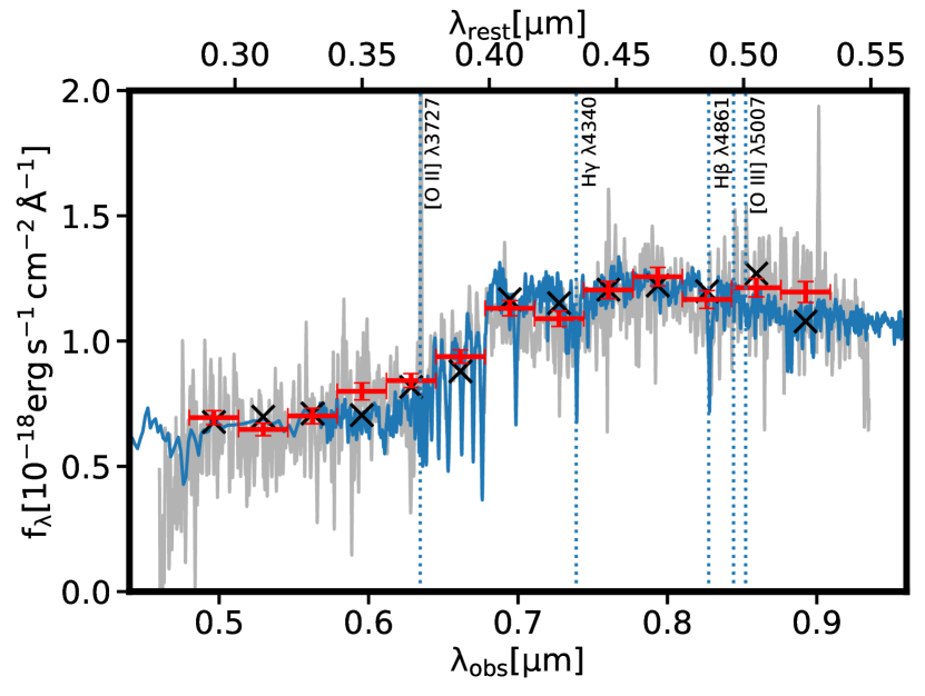
Figure 2: Best-fit SED model (blue) for the main foreground galaxy compared to the observed spectrum (grey, smoothed with $FWHM=8.8\,\textnormal{\AA}$ Gaussian). The fit was done using pseudo-photometry for 13 medium-band filters created from the spectrum itself. The red errorbars indicate the filter-averaged flux densities in these filters, with the horizontal bars indicating the width of the filters. The black crosses show the flux-densities in the same filters as obtained from the best-fit SED. While the SED fitting was done including emission lines and the shown model medium band flux-densities include this contribution, the best-fit SED is shown without the emission to avoid visual confusion with the actual emission lines.

The spectrum of the main $z=0.704$ galaxy is shown in Fig. 2. The galaxy shows visibly weaker line emission than is typical for star-forming galaxies on the star forming “main sequence” (MS) at this redshift (e.g. Speagle et al., 2014; Boogaard et al., 2018). Quantitatively, we found the galaxy to have a stellar mass of $\log(M_{*}/\mathrm{M_{\odot}})=$$9.8_{-0.0}^{+0.4}$ and a star formation rate (SFR) of $0.5_{-0.2}^{+0.3}$$\,\mathrm{M}_{\odot}\,\mathrm{yr}^{-1}$.

The corresponding specific SFR ($\mbox{sSFR}=0.07\pm 0.06\,\mathrm{Gyr}^{-1}$) is $-0.6_{-0.6}^{+0.2}$$\,\mathrm{dex}$ (or $\approx 1.5\sigma$) below the MS prediction for $z=0.70$ (Boogaard et al., 2018). This means our galaxy is similar to ’green valley’ galaxies.

We determined the stellar mass and SFR as in paper II. In short, we estimated $M_{*}$ from SED fitting using our custom code coniecto (see also Zabl et al. 2016) on 13 pseudo-medium band filters created from the MUSE spectrum. Other values obtained from the SED fit are listed in Table 2. The (instantaneous) SFR was determined starting from the measured [Oii] flux, correcting it for extinction using the Calzetti et al. (2000) law with the strength of the extinction estimated from the $M_{*}-E(B-V)$ relation of Garn & Best (2010), and converted to a SFR using the Kewley et al. (2004) relation.

We estimated the [Oii] flux from a fit to the [Oii] morpho-kinematics using the 3D fitting tool galpak3d (Bouché et al., 2015). This fit provided us also with a best-fit estimate of the kinematics (see Table 2). The steps involved in the galpak3d fitting were again identical to those described in paper II. However, as the [Oii] flux is low for this galaxy, it was not possible to robustly measure the kinematics and morphology (inclination in particular) based on [Oii] alone. Thus, we decided to constrain the inclination, $i$, using a continuum map in a pseudo r-band image created from the MUSE cube. We determined the galaxy morphology, including $i$ and position angle, $PA$, from this continuum map using galfit (Peng et al., 2010). Further, we used the appropriate PSF for the r-band as determined from the quasar. The fit was complicated by systematic residuals from the close-by quasar. Nevertheless, we could obtain a robust estimate of $i=71\pm 5\deg$ and $PA=37\,\pm 8\deg$. Details about the fit and the method to estimate the uncertainties are given in Appendix A. Finally, we fit the [Oii] kinematics with galpak3d using $i$ and the $PA$ as obtained from the continuum ($i=71\deg$, $PA=37\deg$).

3.3 Absorption in CGM of the main galaxy

The CGM around the $z=0.704$ main galaxy can be probed in absorption at multiple locations using the spectra of the background quasar and the back1 galaxy. While high spectral resolution spectroscopy is only available for the quasar, we can use the MUSE data cube to probe Mgii absorption with the same spectral resolution in both sightlines.

3.3.1 Mgii absorption at the resolution of MUSE

Mgii is the strongest among the CGM metal absorption lines covered by the MUSE data at this redshift and hence the most useful to probe the CGM with low signal-to-noise (S/N) background galaxy sightlines. We show in panel E of Fig. 1 the observed z=0.704 Mgii absorption both for the quasar (orange) and the back1 (red) sightlines ($\textsc{{\rm Mg}\kern 1.00006pt{\sc ii}}\,\lambda 2796$ -dotted-, $\textsc{{\rm Mg}\kern 1.00006pt{\sc ii}}\,\lambda 2803$ -solid-). The figure shows that Mgii absorption is not only visible in the quasar sightline ($\hbox{$EW_{0}^{\lambda 2796}$}=2.7\,\textnormal{\AA}$), as per selection, but also in the back1 sightline ($\hbox{$EW_{0}^{\lambda 2796}$}=2.0\,\textnormal{\AA}$).

Despite the moderate spectral resolution ($190\,\hbox{km~{}s${}^{-1}$}$ at $4700\,\textnormal{\AA}$), the absorption profiles encode interesting information. First, a velocity shift is clearly visible between the two sightlines. The absorption in the back1 galaxy sightline is redshifted w.r.t. that in the quasar sightline by $84\pm 17\,\hbox{km~{}s${}^{-1}$}$, with the absorption in the two sightlines centred at $110\pm 17\,\hbox{km~{}s${}^{-1}$}$ and $25.8\pm 0.4\,\hbox{km~{}s${}^{-1}$}$, respectively. We obtained these velocity measurements by simultaneously fitting both components of the Mgii doublet with Gaussians. Second, we measured a $EW_{0}^{\lambda 2796}$/$EW_{0}^{\lambda 2803}$ ratio close to one in both sightlines. This means the Mgii absorption is strongly saturated. Third, we find that the flux reaches almost zero at peak absorption. For both sightlines, this means, when accounting for the resolution of MUSE, that the Mgii absorption is spread over a large velocity range. For the extended galaxy sightline (back1), this further means that the Mgii coverage must be complete over the extent of the aperture from which we have extracted the background spectrum. The non-circular extraction aperture, which was chosen to optimize the S/N, included 29 spatial pixels corresponding to an area of $1.2\,\mathrm{arcsec}^{2}$.

3.3.2 Absorption at the resolution of UVES

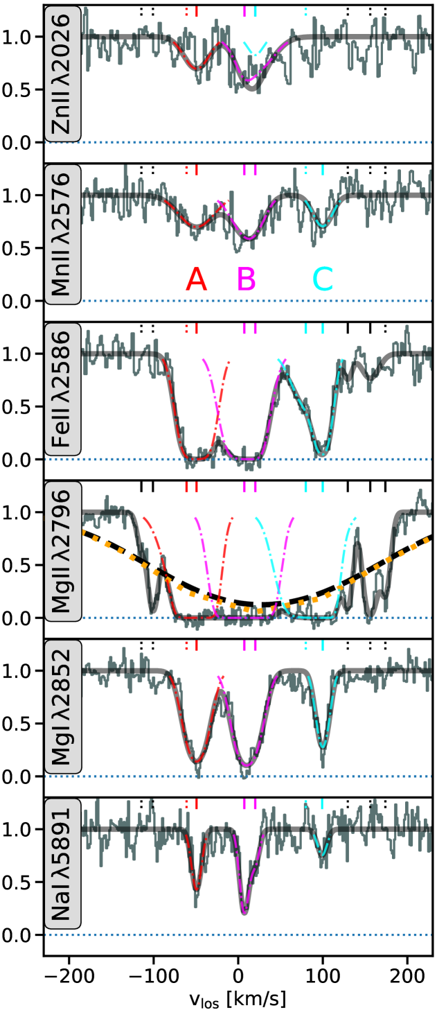
Figure 3: Absorption in the quasar sightline at the redshift of main measured with the high spectral resolution VLT/UVES data. Panels 1-6 from the top: The observed absorption is shown for multiple species, with a multi-component model fit (thick grey line) overplotted over the data. The velocity components considered in the fit are indicated as little bars near the top of the panels, where a dotted bar indicates that the component was not used for the specific line. Three main kinematic components, A, B, C, can be clearly identified from the unsaturated lines. The contribution of the three components, as measured from the multi-component fit, is shown by different colors. For comparison, the panel for $\textsc{{\rm Mg}\kern 1.00006pt{\sc ii}}{}\,\lambda 2796$ also shows the MUSE spectrum (orange dotted; identical to panel E in Fig. 1) and the UVES spectrum artificially degraded to the resolution of MUSE (black dashed).

In the previous section, we compared Mgii absorption along both the galaxy and the quasar sightline at the same moderate spectral resolution of MUSE. For the quasar sightline, we can use the high spectral resolution UVES spectrum ($8\,\hbox{km~{}s${}^{-1}$}$) to study the kinematics in more detail. In Fig. 3, we show one line each for Mnii, Znii, Feii, Mgii, Mgi, Nai. This is a subset of the low ionization lines covered by the UVES spectrum. In addition to the data, a multi-component fit is shown. For this fit, the positions and total number of velocity components in the absorption system were derived from all identified species. Their wavelength positions were then fixed to avoid degeneracy with blended features. For individual elements, only a subset of components was selected and fitted with a single Gaussian each with the evolutionary algorithm described in Quast et al. (2005) and applied in Wendt & Molaro (2012).

As expected from the MUSE spectrum, the $\textsc{{\rm Mg}\kern 1.00006pt{\sc ii}}\,\lambda 2796$ absorption covers a broad velocity range - from $-130$ to $205\,\hbox{km~{}s${}^{-1}$}$ - and is strongly saturated for most of this range. Unsaturated or weakly saturated lines, such as the $\textsc{{\rm Mg}\kern 1.00006pt{\sc i}}\,\lambda 2852$ line, are more useful to identify sub-structures. Based on these transitions, we identified three main components, which are indicated in Fig. 3 and labeled with A (red), B (magenta), and C (orange). They are offset from the systemic redshift of the foreground galaxy by $-49$, $10$, and $100\,\hbox{km~{}s${}^{-1}$}$, respectively.

From the UVES spectrum, [Znii/Feii] is measured for components A$+$B to be $\sim 1.1\pm 0.1$, which indicates a significant amount of depletion for intervening systems (De Cia et al., 2016) of $\approx 0.3$ dex ($\approx 1.5$ dex) for Zn (Fe), respectively. This level of depletion is also associated with more metal rich absorption systems with [Zn/H] around $1/2$ solar (De Cia et al., 2016).

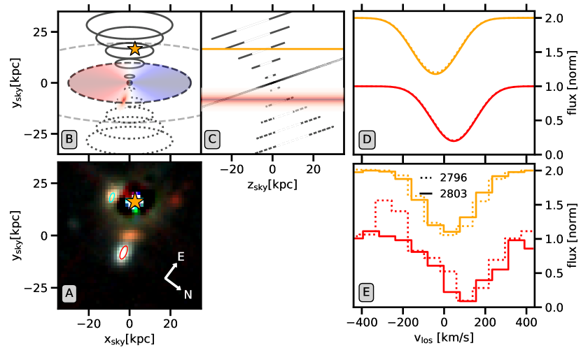
Figure 1: Comparison between data and model for the Mgii absorption seen in the MUSE spectrum for two sightlines through the CGM of the main galaxy. A: $9\arcsec{}.8\times 9\arcsec{}.8$ field, corresponding to $70\ \hbox{kpc}\times 70\,\hbox{kpc}$ at $z=0.70$, around the main foreground galaxy shown as color image with pseudo z’,r’,V broad-band MUSE images in the red, green, and blue channel, respectively. The quasar was subtracted, but residuals are visible. The main foreground galaxy (center) is surrounded by three bright background sources: the quasar towards the top (orange star), the bright galaxy towards the bottom (back1; red ellipse), and the second galaxy close to the quasar (back2; cyan ellipse). B: View of the assumed CGM model (see §4) on the sky plane. The approaching outflow cone is indicated as solid concentric circles, while the receding outflow cone is indicated by dotted circles. For the extended gas disk, the rotation line-of-sight velocity field is overlaid. The orientation is identical to panel A and the positions of the quasar and back1 are indicated by the orange dot and the red surface-brightness ellipse, respectively. C: Geometry of the same model as in B, but here with the line-of-sight direction on the x-axis. The point-source sightline for the quasar (orange) and the extended sightline for back1 (red) are indicated. The cone is hollow in the inner part. D: Mgii$\,\lambda\lambda 2796,2803$ line-of-sight kinematics simulated at the resolution of MUSE based on the model shown in panels B&C and described in §5.3 for the quasar (orange; offset by +1) and back1(red) sightlines, respectively. The model parameters are listed as ’disk + wind’ model in Table 4. E: Mgii line-of-sight kinematics measured with MUSE in the background quasar (orange; offset by +1) and galaxy spectra (red), respectively. Both the $2796\,\textnormal{\AA}$ and $2803\,\textnormal{\AA}$ lines of the Mgii doublet are shown (dotted/solid). The zero-velocity corresponds to the systemic redshift of the main galaxy ($z=0.70344$) as measured from the [Oii] emission.

Table 1: Geometrical orientation of the system. (1) Background object ID; (2) redshift; (3) impact parameter measured from main $z=0.70$ foreground galaxy [kpc at redshift of main]; (4) azimuthal angle w.r.t. the major axis of main [deg]; (5) magnitude in 1″ diameter aperture measured in pseudo-V filter created from MUSE data.

Object	z	b	$\alpha$	$m_{\textnormal{V}}$
(1)	(2)	(3)	(4)	(5)
Quasar	1.48	$16.8\pm 0.7$	$81\pm 8$	18.5
Back1	1.417	$8.8\pm 0.7$	$-109\pm 9$	24.7
Back2	0.809	$20.5\pm 0.7$	$115\pm 8$	24.0

Table 2: Physical properties of the foreground galaxy (main). For further details see §3.2 and paper II. (1) [Oii] flux obtained from galpak3d fit; (2) nebular extinction from $E(B-V)$-$M_{*}$ relation; (3) nebular extinction from SED fit; (4) instantaneous SFR from 1 & 2; (5) instantaneous SFR from SED fit; (6) stellar mass from SED fit; (7) rest-frame B absolute magnitude from best fit SED model; (8) distance from the MS (assuming MS from Boogaard et al. 2018); (9) age of galaxy from SED fit (time since onset of star-formation); (10) decay time in delayed $\tau$ SFH from SED fit; (11) rotation velocity from galpak3d fit; (12) velocity dispersion from galpak3d fit; (13) virial velocity from $v_{\mathrm{vir}}=v_{\mathrm{max}}/(1.1\pm 0.3)$; (14) virial radius from $v_{\mathrm{vir}}$; (15) virial mass from $v_{\mathrm{vir}}$; (16) virial mass from abundance matching (Behroozi et al., 2010); (17) escape velocities at position of quasar/back1 sightline assuming a truncated isothermal sphere.

Row	Property	Value	Unit
(1)	$f_{\textsc{[{\rm O}\kern 0.70004pt{\sc ii}}]}$	$(1.5{\scriptstyle\pm 0.1})\times 10^{-17}$	$\mathrm{erg}\,\mathrm{s}^{-1}\,\mathrm{cm}^{-2}$
(2)	E(B-V) ($M_{*}$)	$0.24_{-0.09}^{+0.12}$	mag
(3)	E(B-V) (SED)	$0.00_{-0.00}^{+0.42}$	mag
(4)	SFR ($f_{\textsc{[{\rm O}\kern 0.70004pt{\sc ii}}]}$)	$0.5_{-0.2}^{+0.3}$	$\mathrm{M}_{\odot}\,\mathrm{yr}^{-1}$
(5)	SFR (SED)	$0.3_{-0.0}^{+9.6}$	$\mathrm{M}_{\odot}\,\mathrm{yr}^{-1}$
(6)	$M_{*}$ (SED)	$9.8_{-0.0}^{+0.4}$	$\log(\mathrm{M_{\odot}})$
(7)	$B$	-19.6	mag
(8)	$\delta(MS)$	$-0.6_{-0.6}^{+0.2}$	dex
(9)	$age$	$9.5_{-0.3}^{+0.0}$	$\log(\mathrm{yr})$
(10)	$\tau$	$8.7_{-0.1}^{+0.6}$	$\log(\mathrm{yr})$
(11)	$v_{\mathrm{max}}$	$118{\scriptstyle\pm 21}$	km s-1
(12)	$\sigma_{0}$	$38{\scriptstyle\pm 15}$	km s-1
(13)	$v_{\mathrm{vir}}$	$107_{-30}^{+44}$	km s-1
(14)	$r_{\mathrm{vir}}$	$120_{-34}^{+50}$	kpc
(15)	$M_{\mathrm{vir}}$ (from $M_{*}$)	$11.6_{-0.1}^{+0.2}$	$\log(\mathrm{M_{\odot}})$
(16)	$M_{\mathrm{vir}}$ (from kin.)	$11.5_{-0.4}^{+0.5}$	$\log(\mathrm{M_{\odot}})$
(17)	$v_{\mathrm{esc}}$ (qso/back1)	261 / 287	km s-1

4 CGM toy model

Mgii absorption around a galaxy is in observations predominantly found either along the galaxy’s minor or major axis (e.g. Bordoloi et al., 2011; Bouché et al., 2012; Kacprzak et al., 2012; Nielsen et al., 2015; Martin et al., 2019), see also paper II and paper III. A natural explanation for this dichotomy is a simple model of a bi-conical outflow perpendicular to the galaxy disk and an extended gaseous disk aligned with the galaxy disk. This picture has gained support both from the theoretical and observational sides, i.e. predictions from cosmological hydro simulations (winds e.g., Dubois & Teyssier 2008; Shen et al. 2012, 2013, disks: e.g., Pichon et al. 2011; Kimm et al. 2011; Shen et al. 2013; Danovich et al. 2015; Stewart et al. 2011; Stewart et al. 2017) and directly observed emission properties of local galaxies (winds: e.g., Veilleux et al. 2005 for a review, disks: e.g., Putman et al. 2009; Wang et al. 2016; Ianjamasimanana et al. 2018).

In the following, we investigate a toy model implementation for kinematics and morphology of a disk$+$outflow model to interpret the observed absorption features in both the quasar and back1 sightlines.

4.1 Model parameters

Table 3: Summary of model parameters in the CGM toy model (cf. §4).

	Property	Description	Unit
Sightline
(1)	$i$	Inclination	[deg]
Biconocial outflow
(2)	$\theta_{\mathrm{out}}$	Outer (half-)cone opening angle	[deg]
(3)	$\theta_{\mathrm{in}}$	Inner (half-)cone opening angle	[deg]
(4)	$v_{\mathrm{out}}$	Outflow velocity	[km s-1]
(5)	$\sigma_{\mathrm{gas}}$	Gas velocity dispersion	[km s-1]
(6)	$\rho_{1}$	Density at norm radius (Mgii)	[$\mathrm{cm}^{-3}$]
Extended gas disk
(7)	$v_{\mathrm{circ}}$	Circular velocity of gas	[km s-1]
(8)	$v_{\mathrm{r}}$	Radial velocity of gas	[km s-1]
(9)	$h_{\mathrm{r}}$	Exponential scale length (radial)	[kpc]
(10)	$h_{\mathrm{z}}$	Exponential scale length (vertical)	[kpc]
(11)	$\sigma_{\mathrm{gas}}$	Gas velocity dispersion	[km s-1]
(12)	$\rho_{0}$	Density at $r=0$ and $z=0$ (Mgii)	[$\mathrm{cm}^{-3}$]

4.1.1 Biconical outflow

For the outflow model, we assume that a galaxy launches winds from its central region into a bi-conical outflow with half-opening angle $\theta_{\mathrm{out}}$. We allow the cone to be devoid of Mgii within an inner opening angle, $\theta_{\mathrm{in}}$, as indicated by larger samples of wind pairs (e.g. papers I & III, Bouché et al. (2012)). For the wind kinematics, we assume that the gas flows outward radially with an outflow velocity, $v_{\mathrm{out}}$, that does not change with distance from the galaxy. From mass conservation, this constant velocity necessitates a radial density $\rho(r)\propto r^{-2}$, which is normalized at 1 kpc with $\rho_{1}\equiv\rho(1\hbox{kpc})$. We also account for random motions of the encountered gas with $\sigma_{\mathrm{gas}}$. Moreover, we assume that the gas does not change its ionization state and that it is smoothly distributed. Thus the wind parameters are $\theta_{\mathrm{out}}$, $\theta_{\mathrm{in}}$, $v_{\mathrm{out}}$ and $\rho_{1}$ and $\sigma_{\mathrm{gas}}$ which are listed Table 3.

The cone opening angle $\theta_{\mathrm{out}}$ is $\approx 30\deg$, and the inner cone is $\theta_{\mathrm{in}}\approx 15\deg$, consistent with typical values in paper III. The outflow velocity $v_{\mathrm{out}}$ is assumed to be $150\,\hbox{km~{}s${}^{-1}$}$, corresponding to the typical $v_{\mathrm{out}}$ in paper III. The intrinsic dispersion $\sigma_{\mathrm{gas}}$ is chosen somewhat arbitrarily to be $10\,\hbox{km~{}s${}^{-1}$}$. All parameters of the fiducial model are summarized in Table 4.

4.1.2 Extended gas disk

However, as the sightlines are at relatively small impact parameters (at $8.8\,\hbox{kpc}$ and $16.8\,\hbox{kpc}$), a contribution from a thick extended gas disk cannot be ruled out. We model this extended gaseous disk as an exponential profile with scale length $h_{\mathrm{r}}$ in radial direction. In the direction perpendicular to the disk (z-direction), we assume an exponentional profile with scale height $h_{\mathrm{z}}$. The gas density is normalized at the disk mid-plane in the disk center with $\rho_{0}$. For the disk’s kinematics, we assume that the gas is rotating parallel to the disk midplane with a circular velocity $v_{\mathrm{circ}}$, which we assume to be identical to $v_{\mathrm{max}}$ from the galaxy rotation. In addition, the gas velocity vector can also have a radial infall component, $v_{\mathrm{r}}$, which is added to the tangential component keeping $v_{\mathrm{circ}}$ constant.  The disk parameters are $v_{\mathrm{circ}}$, $v_{\mathrm{r}}$, $\sigma_{\mathrm{gas}}$, $h_{\mathrm{z}}$ and $\rho_{0}$ which are summarized in Table 3.

The circular velocity $v_{\mathrm{circ}}$ is given by the kinematics of the host galaxy as described in § 3.2. The stellar scale height $h_{z}$ of distant galaxies is typically $1\,kpc$, as suggested by studies of edge-on disks in Hubble deep fields (e.g. Elmegreen & Elmegreen, 2006; Elmegreen et al., 2017). We assume that the extended cool gas disk probed by Mgii has similar scale height ($h_{z}=1\,\hbox{kpc}$). The gas dispersion, $\sigma_{\mathrm{gas}}$, is assumed to be $\sim 10$ km s^-1 appropriate for the temperature of low-ionization gas. The density $\rho_{0}$ will be adjusted in order to match the absorption optical depth for Mgi.

4.2 Simulated absorption lines

We use our code cgmpy to calculate the Mgii absorption profile which the outflow cones and/or the extended gas disk would imprint on a background source. In short, the code calculates for each of small steps ($=1\,\mathrm{pc}$) along the line-of-sight (LOS) the LOS velocity, $v_{\mathrm{los;step}}$, and the column density, $N_{\mathrm{step}}$, which can subsequently be converted to an optical depth, $\tau_{\mathrm{step}}(v_{\mathrm{los}})$. The full $\tau(v_{\mathrm{los}})$ distribution for the complete sightline is then obtained by summing up the $\tau_{\mathrm{step}}(v_{\mathrm{los}})$ from each step and each component without the turbulent velocity dispersion $\sigma_{\mathrm{gas}}$. We account for this random motions of the gas ($\sigma_{\mathrm{gas}}$) by convolving the optical depth distribution with a Gaussian of the selected $\sigma_{\mathrm{gas}}$. Finally, the absorption profile is obtained by taking $e^{-\tau(v_{\mathrm{los}})}$ and convolving with the instrumental line spread function (LSF).

In the case of an extended sightline (such as for ‘back1’), the absorption from the extended object is calculated by taking the average over individual sightlines flux weighted over an elliptical aperture centered on the galaxy (for back1 with an area of $\sim 1\,\mathrm{arcsec}^{2}$).

5 Discussion

Table 4: The choice for each of the parameters in Table 3 as used for the five models described in §5 and shown in Fig. 4.

Model	$i$	$\theta_{\mathrm{out}}$	$\theta_{\mathrm{in}}$	$v_{\mathrm{out}}$	$\sigma_{\mathrm{gas}}$	$\rho_{1}$	$v_{\mathrm{circ}}$	$v_{\mathrm{r}}$	$h_{\mathrm{r}}$	$h_{\mathrm{z}}$	$\sigma_{\mathrm{gas}}$	$\rho_{0}$
	(1)	(2)	(3)	(4)	(5)	(6)	(7)	(8)	(9)	(10)	(11)	(12)
Fiducial wind	71	35	15	150	10	$8\times 10^{-5}$	–	–	–	–	–	–
Slow wind	71	35	15	75	10	$8\times 10^{-5}$	–	–	–	–	–	–
Disk	71	–	–	–	–	–	118	–	5	1	10	$3\times 10^{-3}$
Disk w. infall	71	–	–	–	–	–	118	-40	5	1	10	$3\times 10^{-3}$
Disk + wind	71	35	15	100	10	$8\times 10^{-5}$	118	–	5	1	10	$3\times 10^{-3}$

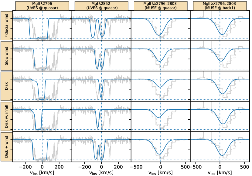
Figure 4: Comparison between data and various models. Eeach row shows a different model, as listed in Table 4. In each panel the light grey curve is the observed absorption, while the blue line shows the modeled absorption. The first two columns show Mgii$\,\lambda 2796$ (column 1) and Mgi$\,\lambda 2852$ (column 2) in the quasar sightline at the resolution of UVES. The third and fourth column show Mgii$\,\lambda 2796,2803$ for the quasar sightline (column 3) and the back1 galaxy sightline (column 4) at the resolution of MUSE. Here, the solid line is Mgii$\,\lambda 2796$ (data and model) and the dotted line is Mgii$\,\lambda 2803$ (data).

Here, we describe how the toy model discussed in §4 performs in discribing our data. However, we stress that we do not expect this simple toy model to account for all data features nor do we attempt to formally fit it to the data. Thus, if the model can, at least approximately, explain most of the absorption in both background sightlines, the simple toy model can be viewed as a description of the main galaxy’s CGM.

5.1 The fiducial (wind-only) model

We first tested the performance of a fiducial biconical outflow-only model (cf. §4.1.1) given that both the quasar and back1 are positionned along the minor axis of the host galaxy, i.e. without an extended gas disk.

Here, the model’s orientation is set by the measurement of the galaxy’s inclination $i$ (see §3.2). However, as the sign of the galaxy inclination cannot be constrained with the available data (see e.g. Ho & Martin, 2019), we were left with two possible solutions. Here, we choose the sign of the inclination such that the absorbing gas in the cones is outflowing. This outflow assumption requires that redshifted absorption must originate from the far-side cone, and consequently, the back1 galaxy sightline crosses this far-side cone. Panels B and C of Fig. 1 show the adopted orientation.

For our ‘fiducial’ outflow model, we assume a value for $\theta_{\mathrm{out}}$ ($35\deg$), which is at the higher end of typical values found in paper III. We made this choice, to ensure very high coverage over the extended back1 galaxy sightline in the model, as required by the observed absorption strength (see §3.3.1).

In Fig. 4 (row 1 - ‘Fiducial wind’), we overlay the resulting absorption profiles over the UVES and MUSE data for the ‘qso’ (Cols 1, 2 and 3) and ‘back1’ (Col. 4) sightlines. Column 1 (2) show the model for the quasar sightlines for Mgii (Mgi), respectively, where we scaled the Mgi density by 1/600 compared to Mgii according to Lan & Fukugita (2017). Comparing our UVES data to the model for the quasar sightlines shown in Cols. 1 ans 2, we find that the absorption is made of two separate components which arise from the assumption of an empty inner cone. These two components might correspond to components A and B in the observed spectrum (see §3.3.2). Comparing our MUSE data and the fiducial wind model (Cols 3 and 4), we find that the model and data match qualitatively for the blue- (red-) shifted absorptions in the quasar (galaxy) sightlines absorption shown in Col. 3 (4), respectively. However, there are some discrepancies between the model and the data.

The main discrepancy is that the wind model cannot explain the redshifted third component C. Another discrepancy is that, for the quasar absorption, the model predicts a blue-shift ($-75$ km s^-1) whereas the observed absorption is close to systemic at $\approx+25$ km s^-1.

A model with lower outflow velocity ($v_{\mathrm{out}}\approx 75\,\hbox{km~{}s${}^{-1}$}$) would better match to components A and B in the Mgi absorption (Fig. 4; row 2 - ‘Slow wind’). However, it under-predicts the redshift compared to the Mgii data in the back1 galaxy sightline. Note that this potential velocity difference between the two sightlines could indicate deceleration of the gas with distance from the galaxy, as the quasar sightline is probing gas at a larger impact parameter than the back1 sightline does ($16.8\,\hbox{kpc}$ vs $8.8\,\hbox{kpc}$). Strong, non-gravitational, deceleration in an outflow could be due to drag forces (in observations e.g., Martini et al. 2018; in simulations e.g., Oppenheimer et al. 2010). However, this interpretation would require the strong assumption that the two opposite cones have the same velocity profile.

5.2 Disk model

Given the limitations of the fiducial wind only-model, and the relatively small impact parameters, we discuss the extended gaseous disk model presented in §4.1.2. Indeed, the two minor-axis sightlines cross the disk midplane at galactocentric radii of $26\,\hbox{kpc}$ ($0.21\,r_{\mathrm{vir}}$) and $51\,\hbox{kpc}$ ($0.42\,r_{\mathrm{vir}}$), within the extent of co-rotating gas disks from paper II and Ho et al. (2017). Before discussing a potential combination of wind and disk-model, we test whether a simple thick disk model similar to Steidel et al. (2002); Kacprzak et al. (2010); Ho et al. (2017) can potentially explain all absorption on its own.

In Fig. 4 (row 3 - ‘Disk’), we overlay the resulting absorption profiles over the MUSE and UVES data as before. Comparing the UVES data to our model shows that a thick disk model can only explain component B in the Mgi spectrum. As for the wind model, the thick disk model cannot explain the redshifted third component C. However, component A in the UVES spectrum could be accounted for with an extension of this disk model with a radial inflow component (shown in row 4 of Fig. 4 - ‘Disk + infall’). The observed velocity of $-49\,\hbox{km~{}s${}^{-1}$}$ would require a radial velocity component of $v_{\mathrm{r}}\approx-40\,\hbox{km~{}s${}^{-1}$}=-0.4\,v_{\mathrm{vir}}$. Such a radial inflow velocity is feasible, based on results from simulations (e.g. Rosdahl & Blaizot, 2012; van de Voort & Schaye, 2012; Goerdt & Ceverino, 2015; Ho et al., 2019) and observational studies targeting the major axis sightlines (e.g. Bouché et al. 2013, 2016; Rahmani et al. 2018a, paper II).

5.3 Combined disk and wind

The observed absorption might be a combination of aborption from both a disk and an outflow component. As discussed in §5.1, the ouflow component alone, a faster wind ($150\,\hbox{km~{}s${}^{-1}$}$) matches better the observed absorption in the back1 sightline, while a slower wind ($75\,\hbox{km~{}s${}^{-1}$}$) matches better the absorption in the qso sightline. For the following, we assume a wind speed of $100\,\hbox{km~{}s${}^{-1}$}$ as a compromise to match approximately both sightlines with a single wind speed. Fig. 4 (row 5 - ‘Disk + wind’) shows the resulting absorption profile when combining the disk and this wind toy model (The same model is also shown in Fig. 1, panel D). While imperfect, the toy model is qualitatively in agreement with the observed spectra, apart from component C. Component C might be an unrelated component, similar to the high-velocity clouds (HVC) seen around the Milky Way (e.g., Wakker & van Woerden 1997 for a review). In summary, a plausible interpretation of the observed kinematics in the two sightlines is absorption in a bi-conical outflow with a potential disk contribution.

5.4 Feasibility of the outflow

As discussed in §3.2, the SFR of the main galaxy is low compared to star-forming galaxies with similar mass at similar redshift. This raises the question whether the energy and the momentum that are required to explain the wind are at all feasible. To answer this question, we estimated the mass outflow rate, $\dot{M}_{\mathrm{out}}$, the energy-outflow rate, $\dot{E}_{\mathrm{out}}$, and the momentum outflow rate, $\dot{p}_{\mathrm{out}}$. These estimates can subsequently be compared to the estimated SFR and the corresponding energy and momentum deposition rates from supernovae (SNe).

We estimated $\dot{M}_{\mathrm{out}}$ for the bi-conical outflow of cool gas using Eq. 5 from paper III. As inputs to the equation we assumed $\theta_{\mathrm{out}}=35\deg$, $\theta_{\mathrm{in}}=15\deg$, $b=15\,\hbox{kpc}$, $v_{\mathrm{out}}=100\,\hbox{km~{}s${}^{-1}$}$, $\log(N_{\textsc{{\rm H}\kern 0.70004pt{\sc i}}}/\mathrm{cm}^{-2})=20.0$. Here, we estimated the Hi column density using the $EW_{0}^{\lambda 2796}$ - Hi relation from Ménard & Chelouche (2009) and Lan & Fukugita (2017), which has an uncertainty of around $0.3\,\mathrm{dex}$. Using these values in the equations we obtain $\dot{M}_{\mathrm{out}}=2.0\,\mathrm{M}_{\odot}\,\mathrm{yr}^{-1}$. This corresponds with the assumed $v_{\mathrm{out}}=100\,\hbox{km~{}s${}^{-1}$}$ to $\dot{E}_{\mathrm{out}}=6.0\times 10^{39}\,\mathrm{erg}\,\mathrm{s}^{-1}$ and $\dot{p}_{\mathrm{out}}=1.3\times 10^{33}\,\mathrm{g}\,\mathrm{cm}\,\mathrm{s}^{-1}$.

A comparison of $\dot{M}_{\mathrm{out}}$ to the estimated SFR allows us to infer the mass-loading ($\eta=\dot{M}_{\mathrm{out}}/\mbox{SFR}$), which characterizes the efficiency of a star formation powered wind to remove gas from the galaxy. Assuming that the wind was powered by the current SFR of $0.5\,\mathrm{M}_{\odot}\,\mathrm{yr}^{-1}$, we infer $\eta\approx 4$. This value can be compared to measurements of $\eta$ both from individual estimates (quasar sightlines e.g. paper III, Bouché et al. 2012; Schroetter et al. 2015; down the barrel: e.g. Weiner et al. 2009; Martin et al. 2012; Rubin et al. 2014; Sugahara et al. 2017), indirect observational evidence (e.g. Zahid et al., 2014; Mitra et al., 2015), or simulations (e.g. Hopkins et al., 2012; Muratov et al., 2015). For the mass and redshift of our main galaxy, the values in these studies typically range from $\eta\approx 1\mbox{--}10$ (see also discussion in paper III). Hence, we conclude that the $\eta$ corresponding to our preferred model seems feasible.

A direct comparison of the measured $\dot{E}_{\mathrm{out}}$ and $\dot{p}_{\mathrm{out}}$ to the momentum and energy injected by SNe leads to a similar conclusion. Per $1\mathrm{M}_{\odot}\,\mathrm{yr}^{-1}$ of star formation SNe deposit mechanical energy and momentum with rates of approximately $1.6\times 3\times 10^{41}\,\mathrm{erg}\,\mathrm{s}^{-1}$ (from Chisholm et al. 2017 based on Leitherer et al. 1999) and $1.6\times 2\times 10^{33}\,\mathrm{g}\,\mathrm{cm}\,\mathrm{s}^{-1}$ (Murray et al. 2005). This means that our measured values correspond to energy and momentum loading of 3% and 80%, respectively. These values are comparable to those found by Chisholm et al. (2017) for a sample of local star-forming galaxies when considering the relevant mass range.

Finally, we note that the actual loading factors could be smaller. The SFR might have been higher at the time when the wind was launched. It would have taken the wind $\approx 200\,\mathrm{Myr}$ ($\approx 100\,\mathrm{Myr}$) to travel to the quasar (back1) sightline, assuming $v_{\mathrm{out}}=100\,\hbox{km~{}s${}^{-1}$}$. With the limited available data we cannot rule out that there was a significant burst of star-formation about $200\mbox{--}300\,\mathrm{Myr}$ ago, as motivated by tests with non-parmetric SFHs with ppxf (Cappellari & Emsellem, 2004; Cappellari, 2017).

6 Conclusions

It is now statistically well established that there is a dichotomy in the spatial distribution of the cool circum-galactic medium (CGM) gas probed through Mgii absorption, where the two components have been identified as arising in an extended gas disk and a bi-conical outflow. In this paper, we present a rare chance alignment of a quasar and a UV-bright background galaxy at relatively small impact parameters ($16.8$ and $8.8\,\hbox{kpc}$) from a $z=0.7$ foreground galaxy. As the two sightlines are close to the foreground galaxy’s projected minor axis, but on opposite sides of the major axis, the configuration is ideal to test the bi-conical outflow component. Through studying the observed absorption both in MUSE and UVES data from the MEGAFLOW survey, and comparison to modeled absorption, we reached the following conclusions:

• Both sightlines show very strong Mgii absorption ($\hbox{$EW_{0}^{\lambda 2796}$}>2.0\,\textnormal{\AA}$).

• We find a significant velocity shift of $84\pm 17\,\hbox{km~{}s${}^{-1}$}$ between the two sightlines.

• The observed velocity shift is in broad agreement with a bi-conical outflow toy model with a moderate outflow velocity of $\approx 100\,\hbox{km~{}s${}^{-1}$}$, possibly combined with a disk model.

• The foreground galaxy has a relatively low sSFR ($0.07\pm 0.06\,\mathrm{Gyr}^{-1}$), which puts the galaxy $0.6\,\mathrm{dex}$ below the MS at $z=0.7$. However, the mass-loading ($\eta$) required to explain the modelled outflow is not unrealistic high ($\eta\approx 4$). Moreover, the sSFR may have been higher when the wind was launched, $\sim 10^{8}\,\mathrm{yr}$.

This study presented a ‘tomographic’ study (i.e. with multi-sightline) of the CGM around an individual galaxy in the distant Universe ($z\approx 0.7$), and hence goes beyond the statistical inference from single sightline samples. While we find the data to be in broad agreement with our fiducial CGM model, we cannot rule out alternative explanations. A comparison of the CGM model to larger samples of rare multi-sightline cases, including cases with even more sightlines as e.g. provided by background groups or gravitationally lensed arcs (e.g. Lopez et al., 2018, 2019), will be an important test for our assumed geometry. Additionally, it will be necessary to test the geometry against observations of the CGM in emission (e.g. Finley et al., 2017; Rupke et al., 2019).

Appendix A Uncertainty on inclination and position angle

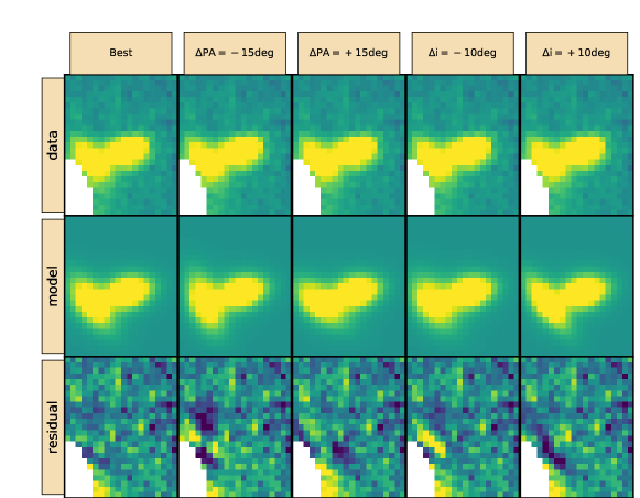
Figure 5: Data, galfit model, and residuals (data-model) are shown for each of five models in the top, center, and bottom row, respectively. The data, which are identical in each of the four columns, are a pseudo broadband r image created from the MUSE cube. The main foreground galaxy is to the left and the back1 background galaxy is to the right (north is to the top, east to the left; different orientation from Fig. 1). The white region to the lower left masks residuals from the quasar subtraction. Left column: Best fit galfit model, where both main and back1 were fit simultaneously. The main galaxy has best fit $PA_{\mathrm{best}}=37\deg$ and $i_{\mathrm{best}}=71\deg$ assuming a $n=1$ Sersic profile. Center left column: This column and the other three columns show the best fit model with either the $PA$ or $i$ of the main galaxy adjusted. Here, $PA=PA_{\mathrm{best}}-15\deg$; Center column: $PA=PA_{\mathrm{best}}+15\deg$; Center right column: $i=i_{\mathrm{best}}-10\deg$; Right column: $i=i_{\mathrm{best}}+10\deg$.

In our analysis, we tied the orientation of our toy model (§4) to the orientation of the main foreground galaxy. Therefore, a robust measurement of position angle ($PA$) and inclination ($i$) is important. As discussed in §3.2, the measurement of the galaxy’s morphology is somewhat complicated by residuals from the PSF subtraction. The residuals made a formal assessment of the uncertainties based on the $\chi^{2}$ doubtful. Therefore, we preferred to rely on a visual assessment of the uncertainties. For this purpose we created galfit models deviating from the best fit model either in $PA$ or inclination. Fig. 5 shows models and residuals all for the best-fit model, the $PA_{\mathrm{best}}-15\deg$, $PA_{\mathrm{best}}+15\deg$, $i_{\mathrm{best}}-10\deg{}$, $i_{\mathrm{best}}+10\deg{}$. Except for the modified $PA$ or $i$, we used in each case identical morphological parameters to those in the best fit model. The only free fit parameter in each of the alternative models was the total flux. Both for $PA\pm 15\deg$ and $i\pm 10\deg$ the residuals are much stronger than for the best-fit model and the models seems essentially inconsistent with the data. Therefore, it seems plausible to define these $PA$ and $incl$ differences as $2\sigma$ uncertainties. In summary, we conclude therefore that the $1\sigma$ uncertainties for $PA$ and $i$ are $8\deg$ and $5\deg$, respectively.

In addition to the uncertainty in $PA$ and $i$, there is also a small uncertainty on the centroid. We estimated this uncertainty through comparison between the continuum centroid obtained from this galfit fit and the [Oii] centroid obtained from galpak3d fit. We find a deviation of $0\arcsec.16$ between the two centroids. Therefore, we can assume as $1\sigma$ uncertainty $0\arcsec.1$ both in right ascension and declination.

Appendix B Impact of uncertainties on inclination and position angle on models

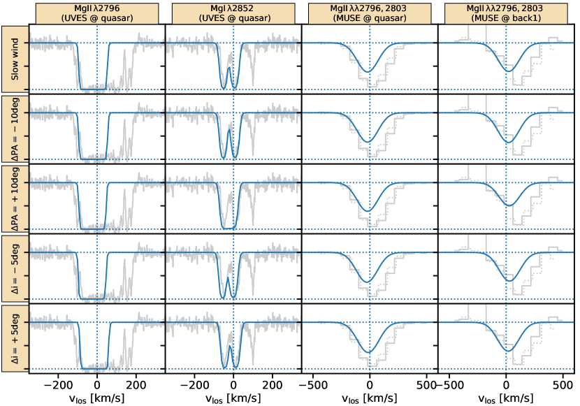
Figure 6: Comparison between modeled and observed absorption for the ‘Slow wind’ model assuming different inclinations and position angles. The first row is identical to row 2 in Fig. 4, where the best fit $i$ and $PA$ were assumed. Details about the content displayed in the four columns are given in the caption of Fig. 4. The subsequent rows (1-4) show the same model, but with $i$ or $PA$ changed by the values stated in the row labels. For further details, see Appendix B.

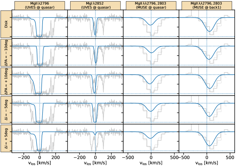
Figure 7: As Fig. 6, but here for the ‘Disk’ model (cf. row 3 in Fig. 4). For further details, see Appendix B.

In this section, we asses the impact of the uncertainties for $i$ and $PA$ on the simulated absorption in our toy models.

In Fig. 6 we show the ‘Slow wind’ model (see. Table 4) with either $i$ or $PA$ changed compared to the fiducial values (row 1). Rows 2 and 3 show the result for changing the $i$ by $\pm 5\deg$ (i.e., $66\deg$ and $76\deg$), while keeping the fiducial value for the $PA$. Rows 4 and 5 show the impact of varying the $PA$ of main by $\pm 10\deg$. Assuming $\Delta PA\pm 10\deg$ means that the azimuthal angle $\alpha$ is changed by $\mp 10\deg$ both for the quasar and the back1 sightline (equally) compared to the values stated in Table 1. All other parameters are kept identical to those listed for the ‘Slow wind’ model in Table 4 and shown in the first row of Fig. 6.

In general, the differences between the absorption profiles for these variants appear small. The strongest visible impact is for $\Delta PA=+10\deg$ (corresponding to $\alpha=71\deg$ for quasar and $\alpha=-119\deg$ for back1). In this case, the Mgi absorption profile is not double-peaked and the Mgii absorption in the back1 sightline is visibly weaker than in the fiducial model. The double peak is absent, because the distance from the minor axis is larger than in the fiducial case and, consequently, the quasar sightline does not cross the hollow part of the cone. The weaker Mgii absorption for back1 is also a consequence of a larger distance from the minor axis. At $\alpha=-119\deg$ part of the extended back1 galaxy sightline is no longer covered by the cone at all, which reduces the effective $EW_{0}^{\lambda 2796}$.

In Fig 7, we test the impact of the same $i$ and $PA$ variations, but now for the ‘Disk’ model (see Table 4). Here, the differences in absorption strength appear stronger than in the wind case. This is especially the case for changes in $i$. Here, the strength varies - especially for the Mgi absorption in the quasar sightline - as the sightline crosses the disk mid-plane at larger galacto-centric radii, the larger the $i$ is. We note, though, that most of the changes could be compensated for by merely choosing a disk with higher density. For the variations with $PA$, the centroid of the absorption shifts, but only slightly.

In summary, we can conclude that the uncertainties on $i$ and $PA/\alpha$, as estimated in Appendix A, only subtly change our simulated profiles. Therefore, we can conclude that our conclusions in §5 are not impacted by these uncertainties.

References

- Astropy Collaboration et al. (2013) Astropy Collaboration et al., 2013, A&A, 558, A33
- Bacon et al. (2006) Bacon R., et al., 2006, Msngr, 124, 5
- Bacon et al. (2010) Bacon R., et al., 2010, in Society of Photo-Optical Instrumentation Engineers (SPIE) Conference Series. p. 8, doi:10.1117/12.856027
- Bacon et al. (2017) Bacon R., et al., 2017, A&A, 608, A1
- Behroozi et al. (2010) Behroozi P. S., Conroy C., Wechsler R. H., 2010, ApJ, 717, 379
- Bergeron (1988) Bergeron J., 1988, in IAU Symp. 130: Large Scale Structures of the Universe. pp 343–+
- Bergeron & Boissé (1991) Bergeron J., Boissé P., 1991, A&A, 243, 344
- Bergeron & Stasińska (1986) Bergeron J., Stasińska G., 1986, A&A, 169, 1
- Boogaard et al. (2018) Boogaard L. A., et al., 2018, A&A, 619, A27
- Bordoloi et al. (2011) Bordoloi R., et al., 2011, ApJ, 743, 10
- Bouché et al. (2006) Bouché N., Murphy M. T., Péroux C., Csabai I., Wild V., 2006, MNRAS, 371, 495
- Bouché et al. (2012) Bouché N., Hohensee W., Vargas R., Kacprzak G. G., Martin C. L., Cooke J., Churchill C. W., 2012, MNRAS, 426, 801
- Bouché et al. (2013) Bouché N., Murphy M. T., Kacprzak G. G., Péroux C., Contini T., Martin C. L., Dessauges-Zavadsky M., 2013, Science, 341, 50
- Bouché et al. (2015) Bouché N., Carfantan H., Schroetter I., Michel-Dansac L., Contini T., 2015, AJ, 150, 92
- Bouché et al. (2016) Bouché N., et al., 2016, ApJ, 820, 121
- Bowen et al. (2016) Bowen D. V., Chelouche D., Jenkins E. B., Tripp T. M., Pettini M., York D. G., Frye B. L., 2016, ApJ, 826, 50
- Calzetti et al. (2000) Calzetti D., Armus L., Bohlin R. C., Kinney A. L., Koornneef J., Storchi-Bergmann T., 2000, ApJ, 533, 682
- Cappellari (2017) Cappellari M., 2017, MNRAS, 466, 798
- Cappellari & Emsellem (2004) Cappellari M., Emsellem E., 2004, PASP, 116, 138
- Chabrier (2003) Chabrier G., 2003, PASP, 115, 763
- Chen et al. (2005) Chen H.-W., Kennicutt Jr. R. C., Rauch M., 2005, ApJ, 620, 703
- Chen et al. (2010) Chen H.-W., Helsby J. E., Gauthier J.-R., Shectman S. A., Thompson I. B., Tinker J. L., 2010, ApJ, 714, 1521
- Chisholm et al. (2017) Chisholm J., Tremonti C. A., Leitherer C., Chen Y., 2017, MNRAS, 469, 4831
- Crighton et al. (2010) Crighton N. H. M., Morris S. L., Bechtold J., Crain R. A., Jannuzi B. T., Shone A., Theuns T., 2010, MNRAS, 402, 1273
- D’Odorico et al. (1998) D’Odorico V., Cristiani S., D’Odorico S., Fontana A., Giallongo E., Shaver P., 1998, A&A, 339, 678
- Dahlen et al. (2007) Dahlen T., Mobasher B., Dickinson M., Ferguson H. C., Giavalisco M., Kretchmer C., Ravindranath S., 2007, ApJ, 654, 172
- Danovich et al. (2015) Danovich M., Dekel A., Hahn O., Ceverino D., Primack J., 2015, MNRAS, 449, 2087
- De Cia et al. (2016) De Cia A., Ledoux C., Mattsson L., Petitjean P., Srianand R., Gavignaud I., Jenkins E. B., 2016, A&A, 596, A97
- Dekker et al. (2000) Dekker H., D’Odorico S., Kaufer A., Delabre B., Kotzlowski H., 2000, in Iye M., Moorwood A. F., eds, Proc. SPIEVol. 4008, Optical and IR Telescope Instrumentation and Detectors. pp 534–545, doi:10.1117/12.395512
- Dubois & Teyssier (2008) Dubois Y., Teyssier R., 2008, A&A, 477, 79
- Ellison et al. (2004) Ellison S. L., Ibata R., Pettini M., Lewis G. F., Aracil B., Petitjean P., Srianand R., 2004, A&A, 414, 79
- Elmegreen & Elmegreen (2006) Elmegreen B. G., Elmegreen D. M., 2006, ApJ, 650, 644
- Elmegreen et al. (2017) Elmegreen B. G., Elmegreen D. M., Tompkins B., Jenks L. G., 2017, ApJ, 847, 14
- Finley et al. (2017) Finley H., et al., 2017, A&A, 605, A118
- Garn & Best (2010) Garn T., Best P. N., 2010, MNRAS, 409, 421
- Goerdt & Ceverino (2015) Goerdt T., Ceverino D., 2015, MNRAS, 450, 3359
- Ho & Martin (2019) Ho S. H., Martin C. L., 2019, arXiv e-prints, p. arXiv:1901.11182
- Ho et al. (2017) Ho S. H., Martin C. L., Kacprzak G. G., Churchill C. W., 2017, ApJ, 835, 267
- Ho et al. (2019) Ho S. H., Martin C. L., Turner M. L., 2019, ApJ, 875, 54
- Hopkins et al. (2012) Hopkins P. F., Quataert E., Murray N., 2012, MNRAS, 421, 3522
- Hunter (2007) Hunter J. D., 2007, Computing in Science and Engineering, 9, 90
- Ianjamasimanana et al. (2018) Ianjamasimanana R., Walter F., de Blok W. J. G., Heald G. H., Brinks E., 2018, AJ, 155, 233
- Jenkins (2009) Jenkins E. B., 2009, ApJ, 700, 1299
- Kacprzak et al. (2010) Kacprzak G. G., Churchill C. W., Ceverino D., Steidel C. C., Klypin A., Murphy M. T., 2010, ApJ, 711, 533
- Kacprzak et al. (2011a) Kacprzak G. G., Churchill C. W., Evans J. L., Murphy M. T., Steidel C. C., 2011a, MNRAS, 416, 3118
- Kacprzak et al. (2011b) Kacprzak G. G., Churchill C. W., Barton E. J., Cooke J., 2011b, ApJ, 733, 105
- Kacprzak et al. (2012) Kacprzak G. G., Churchill C. W., Nielsen N. M., 2012, ApJ, 760, L7
- Kacprzak et al. (2014) Kacprzak G. G., et al., 2014, ApJ, 792, L12
- Kewley et al. (2004) Kewley L. J., Geller M. J., Jansen R. A., 2004, AJ, 127, 2002
- Kimm et al. (2011) Kimm T., Devriendt J., Slyz A., Pichon C., Kassin S. A., Dubois Y., 2011, preprint, (arXiv:1106.0538)
- Lan & Fukugita (2017) Lan T.-W., Fukugita M., 2017, ApJ, 850, 156
- Lan & Mo (2018) Lan T.-W., Mo H., 2018, ApJ, 866, 36
- Lan et al. (2014) Lan T.-W., Ménard B., Zhu G., 2014, ApJ, 795, 31
- Lanzetta & Bowen (1990) Lanzetta K. M., Bowen D., 1990, ApJ, 357, 321
- Lanzetta et al. (1987) Lanzetta K. M., Turnshek D. A., Wolfe A. M., 1987, ApJ, 322, 739
- Leitherer et al. (1999) Leitherer C., et al., 1999, ApJS, 123, 3
- Lodders (2003) Lodders K., 2003, ApJ, 591, 1220
- Lopez et al. (1999) Lopez S., Reimers D., Rauch M., Sargent W. L. W., Smette A., 1999, ApJ, 513, 598
- Lopez et al. (2007) Lopez S., Ellison S., D’Odorico S., Kim T. S., 2007, A&A, 469, 61
- Lopez et al. (2018) Lopez S., et al., 2018, Nature, 554, 493
- Lopez et al. (2019) Lopez S., et al., 2019, arXiv e-prints, p. arXiv:1911.04809
- Martin et al. (2012) Martin C. L., Shapley A. E., Coil A. L., Kornei K. A., Bundy K., Weiner B. J., Noeske K. G., Schiminovich D., 2012, ApJ, 760, 127
- Martin et al. (2019) Martin C. L., Ho S. H., Kacprzak G. G., Churchill C. W., 2019, ApJ, 878, 84
- Martini et al. (2018) Martini P., Leroy A. K., Mangum J. G., Bolatto A., Keating K. M., Sandstrom K., Walter F., 2018, ApJ, 856, 61
- Ménard & Chelouche (2009) Ménard B., Chelouche D., 2009, MNRAS, 393, 808
- Mitra et al. (2015) Mitra S., Davé R., Finlator K., 2015, MNRAS, 452, 1184
- Muratov et al. (2015) Muratov A. L., Kereš D., Faucher-Giguère C.-A., Hopkins P. F., Quataert E., Murray N., 2015, MNRAS, 454, 2691
- Murray et al. (2005) Murray N., Quataert E., Thompson T. A., 2005, ApJ, 618, 569
- Muzahid (2014) Muzahid S., 2014, ApJ, 784, 5
- Muzahid et al. (2015) Muzahid S., Kacprzak G. G., Churchill C. W., Charlton J. C., Nielsen N. M., Mathes N. L., Trujillo-Gomez S., 2015, ApJ, 811, 132
- Nestor et al. (2005) Nestor D. B., Turnshek D. A., Rao S. M., 2005, ApJ, 628, 637
- Nielsen et al. (2013a) Nielsen N. M., Churchill C. W., Kacprzak G. G., Murphy M. T., 2013a, ApJ, 776, 114
- Nielsen et al. (2013b) Nielsen N. M., Churchill C. W., Kacprzak G. G., 2013b, ApJ, 776, 115
- Nielsen et al. (2015) Nielsen N. M., Churchill C. W., Kacprzak G. G., Murphy M. T., Evans J. L., 2015, ApJ, 812, 83
- Oliphant (2007) Oliphant T. E., 2007, Computing in Science and Engineering, 9, 10
- Oppenheimer et al. (2010) Oppenheimer B. D., Davé R., Kereš D., Fardal M., Katz N., Kollmeier J. A., Weinberg D. H., 2010, MNRAS, 406, 2325
- Peng et al. (2010) Peng C. Y., Ho L. C., Impey C. D., Rix H.-W., 2010, AJ, 139, 2097
- Péroux et al. (2018) Péroux C., Rahmani H., Arrigoni Battaia F., Augustin R., 2018, MNRAS, 479, L50
- Pichon et al. (2011) Pichon C., Pogosyan D., Kimm T., Slyz A., Devriendt J., Dubois Y., 2011, MNRAS, 418, 2493
- Piqueras et al. (2017) Piqueras L., Conseil S., Shepherd M., Bacon R., Leclercq F., Richard J., 2017, preprint, (arXiv:1710.03554)
- Putman et al. (2009) Putman M. E., et al., 2009, ApJ, 703, 1486
- Quast et al. (2005) Quast R., Baade R., Reimers D., 2005, A&A, 431, 1167
- Rahmani et al. (2018a) Rahmani H., et al., 2018a, MNRAS, 474, 254
- Rahmani et al. (2018b) Rahmani H., et al., 2018b, MNRAS, 480, 5046
- Rauch et al. (1999) Rauch M., Sargent W. L. W., Barlow T. A., 1999, ApJ, 515, 500
- Rosdahl & Blaizot (2012) Rosdahl J., Blaizot J., 2012, MNRAS, 423, 344
- Rubin et al. (2014) Rubin K. H. R., Prochaska J. X., Koo D. C., Phillips A. C., Martin C. L., Winstrom L. O., 2014, ApJ, 794, 156
- Rubin et al. (2018) Rubin K. H. R., et al., 2018, ApJ, 859, 146
- Rupke et al. (2019) Rupke D. S. N., et al., 2019, Nature, 574, 643
- Salpeter (1955) Salpeter E. E., 1955, ApJ, 121, 161
- Schroetter et al. (2015) Schroetter I., Bouché N., Péroux C., Murphy M. T., Contini T., Finley H., 2015, ApJ, 804, 83
- Schroetter et al. (2016) Schroetter I., et al., 2016, ApJ, 833, 39
- Schroetter et al. (2019) Schroetter I., et al., 2019, MNRAS, 490, 4368
- Shen et al. (2012) Shen S., Madau P., Aguirre A., Guedes J., Mayer L., Wadsley J., 2012, ApJ, 760, 50
- Shen et al. (2013) Shen S., Madau P., Guedes J., Mayer L., Prochaska J. X., Wadsley J., 2013, ApJ, 765, 89
- Soto et al. (2016) Soto K. T., Lilly S. J., Bacon R., Richard J., Conseil S., 2016, ZAP: Zurich Atmosphere Purge, Astrophysics Source Code Library (ascl:1602.003)
- Speagle et al. (2014) Speagle J. S., Steinhardt C. L., Capak P. L., Silverman J. D., 2014, ApJS, 214, 15
- Steidel (1995) Steidel C. C., 1995, in Meylan G., ed., QSO Absorption Lines. ESO Astrophysics Symposia. Springer-Verlag, Berlin, Germany, p. 139
- Steidel & Sargent (1992) Steidel C. C., Sargent W. L. W., 1992, ApJS, 80, 1
- Steidel et al. (2002) Steidel C. C., Kollmeier J. A., Shapley A. E., Churchill C. W., Dickinson M., Pettini M., 2002, ApJ, 570, 526
- Stewart et al. (2011) Stewart K. R., Kaufmann T., Bullock J. S., Barton E. J., Maller A. H., Diemand J., Wadsley J., 2011, ApJ, 738, 39
- Stewart et al. (2017) Stewart K. R., et al., 2017, ApJ, 843, 47
- Sugahara et al. (2017) Sugahara Y., Ouchi M., Lin L., Martin C. L., Ono Y., Harikane Y., Shibuya T., Yan R., 2017, ApJ, 850, 51
- Tumlinson et al. (2017) Tumlinson J., Peeples M. S., Werk J. K., 2017, Annual Review of Astronomy and Astrophysics, 55, 389
- Veilleux et al. (2005) Veilleux S., Cecil G., Bland-Hawthorn J., 2005, ARA&A, 43, 769
- Wakker & van Woerden (1997) Wakker B. P., van Woerden H., 1997, ARA&A, 35, 217
- Wang et al. (2016) Wang J., Koribalski B. S., Serra P., van der Hulst T., Roychowdhury S., Kamphuis P., Chengalur J. N., 2016, MNRAS, 460, 2143
- Weilbacher et al. (2012) Weilbacher P. M., Streicher O., Urrutia T., Jarno A., Pécontal-Rousset A., Bacon R., Böhm P., 2012, in Society of Photo-Optical Instrumentation Engineers (SPIE) Conference Series. p. 0, doi:10.1117/12.925114
- Weilbacher et al. (2014) Weilbacher P. M., Streicher O., Urrutia T., Pécontal-Rousset A., Jarno A., Bacon R., 2014, in Manset N., Forshay P., eds, Astronomical Society of the Pacific Conference Series Vol. 485, Astronomical Data Analysis Software and Systems XXIII. p. 451 (arXiv:1507.00034)
- Weilbacher et al. (2016) Weilbacher P. M., Streicher O., Palsa R., 2016, MUSE-DRP: MUSE Data Reduction Pipeline, Astrophysics Source Code Library (ascl:1610.004)
- Weiner et al. (2009) Weiner B. J., et al., 2009, ApJ, 692, 187
- Wendt & Molaro (2012) Wendt M., Molaro P., 2012, A&A, 541, A69
- Zabl et al. (2016) Zabl J., Freudling W., Møller P., Milvang-Jensen B., Nilsson K. K., Fynbo J. P. U., Le Fèvre O., Tasca L. A. M., 2016, A&A, 590, A66
- Zabl et al. (2019) Zabl J., et al., 2019, MNRAS, 485, 1961
- Zahid et al. (2014) Zahid H. J., Torrey P., Vogelsberger M., Hernquist L., Kewley L., Davé R., 2014, Ap&SS, 349, 873
- Zhu & Ménard (2013) Zhu G., Ménard B., 2013, ApJ, 770, 130
- van de Voort & Schaye (2012) van de Voort F., Schaye J., 2012, MNRAS, 423, 2991
- van der Walt et al. (2011) van der Walt S., Colbert S. C., Varoquaux G., 2011, Computing in Science and Engineering, 13, 22