Traveling wave solutions of some important Wick-type fractional stochastic nonlinear partial differential equations

Abstract

In this article, exact traveling wave solutions of a Wick-type stochastic nonlinear Schrödinger equation and of a Wick-type stochastic fractional Regularized Long Wave-Burgers (RLW-Burgers) equation have been obtained by using an improved computational method. Specifically, the Hermite transform is employed for transforming Wick-type stochastic nonlinear partial differential equations into deterministic nonlinear partial differential equations with integral and fraction order. Furthermore, the required set of stochastic solutions in the white noise space is obtained by using the inverse Hermite transform. Based on the derived solutions, the dynamics of the considered equations are performed with some particular values of the physical parameters. The results reveal that the proposed improved computational technique can be applied to solve various kinds of Wick-type stochastic fractional partial differential equations.

Keywords: Wick-type stochastic nonlinear Schrödinger equation; Wick-type stochastic fractional RLW-Burgers equation; Travelling wave solutions; Hermite transform; Solitary waves.

1 Introduction

Stochastic nonlinear partial differential equations play an important role in various fields of science and engineering [1, 2, 3]. In general, finding solutions of stochastic nonlinear partial differential equations is more complex due to its additional random terms when compared to deterministic partial differential equations [4, 5, 6, 7]. In particular, the exact traveling wave solution receives a great deal of attention since it reveals the internal mechanism of physical phenomena and also it can be used to assist numerical solvers to compare the correctness of their results. In particular, the study on obtaining exact traveling wave solutions of stochastic nonlinear partial differential equations via computational techniques is still in the initial stage. At present, only few works have been reported regarding the exact traveling wave solutions of stochastic nonlinear partial differential equations [8, 9, 10, 11, 12, 13]. Saha Ray and Singh obtained new exact solutions of the Wick-type stochastic Kudryashov–Sinelshchikov equation with the aid of improved Sub-equation method [14]. In addition, exact traveling wave solutions for the Wick-type stochastic coupled KdV-mKdV equations have been obtained by employing the Jacobian elliptic function expansion method in [15].

Consider the variable coefficient nonlinear Schrödinger equation in the following form:

$$i\psi_{t}+\alpha(t)\psi_{xx}+\beta(t)\psi|\psi|^{2}+\lambda(t)\psi=0,\quad i^{2}=-1,$$ (1)

which is used to describe a variety of significant phenomena in ocean dynamics, fluid mechanics and plasma physics. Here, $(x,t)\in\mathbb{R}\times\mathbb{R}^{+}$; $\alpha(t),\beta(t)$ and $\lambda(t)$ are bounded measurable or integrable functions on $\mathbb{R}^{+}$ [16, 17]. Based on Eq. (1), we consider the Wick-type stochastic nonlinear Shrödinger equation in form

$$i\Psi_{t}+\alpha^{*}(t)\diamondsuit\Psi_{xx}+\beta^{*}(t)\diamondsuit\Psi\diamondsuit|\Psi|^{\diamondsuit 2}+\lambda^{*}(t)\diamondsuit\Psi=0,$$ (2)

where $\diamondsuit$ is the Wick product on the Kondratiev distribution space $(S(\mathbb{R}^{d}))^{*}$ and $\alpha^{*}(t)$, $\beta^{*}(t)$ and $\lambda^{*}(t)$ are white noise functionals defined in $(S(\mathbb{R}^{d}))^{*}$, where $(S(\mathbb{R}^{d}))^{*}$ is the white noise functional space [18, 19, 20, 21].

On the other hand, fractional calculus is devoted to the study of integrals and derivatives of fractional order, which has been used to describe nonlinear physical models arising in real world problems such as in viscoelastic systems, complex biological systems, signal processing control and image processing of computer vision [22, 23, 24, 25, 26, 27, 28]. Fractional nonlinear partial differential equations (Fractional NPDEs) can be written as generalizations of classical NPDEs through several senses of fractional derivatives [29, 30, 31, 32, 33], including the recent popular one called the Atangana–Baleanu fractional derivative in Caputo sense, which was introduced in [34]. It should be noted that fractional NPDEs can characterize the physical phenomena better than deterministic NPDEs [35, 36]. In particular, it should be noted that it is more difficult to solve stochastic NPDEs in comparison with deterministic NPDEs. Though exact traveling wave solutions of Wick-type stochastic NPDEs have been extensively studied by many researchers, finding exact traveling wave solutions of fractional versions of them is still in the initial stage. Motivated by this consideration, in this paper we consider the fractional Regularized Long Wave-Burgers equation (RLW-Burgers) with Burgers-type dissipative and dispersive terms in the form

$$\frac{\partial^{\alpha}V}{\partial t^{\alpha}}+p(t)\frac{\partial^{\alpha}V}{\partial x^{\alpha}}+q(t)V\frac{\partial^{\alpha}V}{\partial x^{\alpha}}+r(t)\frac{\partial^{2\alpha}V}{\partial x^{2\alpha}}+s(t)\frac{\partial^{3\alpha}V}{\partial t^{\alpha}\partial x^{2\alpha}}=0,$$ (3)

where $p(t)$, $q(t)$, $r(t)$ and $s(t)$ are bounded measurable functions on $\mathbb{R}^{+}$ and the fractional order $\alpha$ belongs to $(0,1)$ [36, 37].

Motivated by Eq. (3), in this paper we consider the Wick-type fractional stochastic version of Eq. (3) in the following form:

$$\frac{\partial^{\diamondsuit\alpha}V}{\partial t^{\diamondsuit\alpha}}+P(t)\diamondsuit\frac{\partial^{\diamondsuit\alpha}V}{\partial x^{\diamondsuit\alpha}}+Q(t)\diamondsuit V\diamondsuit\frac{\partial^{\diamondsuit\alpha}V}{\partial x^{\diamondsuit\alpha}}+R(t)\diamondsuit\frac{\partial^{\diamondsuit 2\alpha}V}{\partial x^{\diamondsuit 2\alpha}}+S(t)\diamondsuit\frac{\partial^{\diamondsuit 3\alpha}V}{\partial t^{\diamondsuit\alpha}\partial x^{\diamondsuit 2\alpha}}=0,$$ (4)

where “$\diamondsuit$” is the Wick product on the Kondratiev distribution space $(S(\mathbb{R}^{d}))^{*}$, and $P(t),Q(t),R(t)$ and $S(t)$ are white noise functionals defined in $(S(\mathbb{R}^{d}))^{*}$ [38]. Also, $P(t)=f_{1}(t)+c_{1}W(t)$, $Q(t)=f_{2}(t)+c_{2}W(t)$, $R(t)=f_{3}(t)+c_{3}W(t)$, $S(t)=f_{4}(t)+c_{4}W(t)$ and $\left\{f_{i}(t)\right\}_{i=1}^{4}$ are bounded and integrable functions on $\mathbb{R}^{+}$, where $\left\{c_{i}\right\}_{i=1}^{4}$ denote constants and $W(t)$ is the Gaussian white noise that satisfies $W(t)=\dot{B}_{t}=dB(t)/dt$ where $B(t)$ is a Brownian motion.

The main aim of this work is to obtain new Wick-type exact traveling wave solutions for Eq. (2) and Eq. (4) by using the improved computational algorithm and the modified fractional sub-equation method. Further, we obtain the white noise functional solutions of Eq. (4) based on the Hermite transform and the Caputo fractional derivative. This paper is organized as follows. In Section 2, we describe the Wick-type product and the improved computational algorithm and we obtain new Wick-type exact traveling wave solutions of the Wick-type stochastic nonlinear Schrödinger equations, and we perform the dynamics of the given solutions of the considered equation. In Section 3, we describe the modified fractional sub-equation method and we present new Wick-type exact traveling wave solutions of Wick-type stochastic fractional RLW-Burgers equations. Finally, some conclusions are presented at the end of the paper in Section 4.

2 Wick-type stochastic nonlinear Schrödinger Equation

Let the space $(S)_{-1}^{n}$ consists of all formal expansions $F(z)=\sum_{\alpha}a_{\alpha}H_{\alpha}(z)$ with $a_{\alpha}\in\mathbb{R}^{n}$ and $z=(z_{1},\ldots,z_{n})\in\mathbb{C}^{n}$ (the set of all sequences of complex numbers).

2.1 Mathematical Computation scheme with Wick product

We define the Wick product of two elements $F=\sum_{\alpha}a_{\alpha}H_{\alpha}$ and $G=\sum_{\beta}b_{\beta}H_{\beta}\in(S)_{-1}^{n}$ with $a_{\alpha},b_{\beta}\in\mathbb{R}^{n}$ by

$$F\diamondsuit G=\sum_{\alpha,\beta}(a_{\alpha},b_{\beta})H_{\alpha+\beta}.$$

For $F=\sum_{\alpha}a_{\alpha}H_{\alpha}\in(S)_{-1}^{n}$, with $a_{\alpha}\in\mathbb{R}^{n}$, the Hermite transform of $F$, denoted by $\mathcal{H}(F)$ or $\tilde{F}(z)$ is defined by

$$\mathcal{H}(F)=\tilde{F}(z)=\sum a_{\alpha}z^{\alpha}\in\mathbb{C}^{n}\ \ (\textrm{when}\mbox{~{}}\textrm{convergent}),$$

where $z=(z_{1},z_{2},\ldots)\in\mathbb{C}^{n}$ and $z^{\alpha}=(z_{1}^{\alpha_{1}},z_{2}^{\alpha_{2}}\ldots)$ for $\alpha=(\alpha_{1},\alpha_{2},\ldots)\in J$, where $z_{j}^{0}=1$.

By the above definition, for $F,G\in(S)_{-1}^{n}$, we have

$$\widetilde{F\diamondsuit G}(z)={\tilde{F}}(z)\dot{\tilde{G}}(z)$$

for all $z$ such that ${\tilde{F}}(z)$ and ${\tilde{G}}(z)$ exist, where the product on the right hand side of the above equation is the complex bilinear product between two elements of $\mathbb{C}^{n}$ defined by $(z_{1}^{\alpha_{1}}\ldots\,z_{n}^{\alpha_{1}})\cdot(z_{1}^{\alpha_{2}}\ldots\,z_{n}^{\alpha_{2}})=\sum_{k=1}^{n}z_{k}^{\alpha_{1}}z_{k}^{\alpha_{2}}$, where $z_{k}^{\alpha_{i}}\in\mathbb{C}$.

We next present the main steps of finding exact solutions of the Wick-type stochastic nonlinear partial differential equations.

Consider nonlinear stochastic partial differential equation in the following form

$$\mathcal{P}(t,x,\partial_{t},\nabla_{x},U,z)=0$$

where $\mathcal{P}$ is some given function, $U=U(t,x,z)$ is the unknown solution, and the operators are $\partial_{t}=\frac{\partial}{\partial t}$, $\nabla_{x}=\left(\frac{\partial}{\partial x_{1}},\ldots,\frac{\partial}{\partial x_{d}}\right)$ when $x=(x_{1},\ldots,x_{d})\in\mathbb{R}^{d}$.

Suppose all functions and all products are interpreted as the Wick products and the Wick versions. Eq. (2.1) can be written in the form

$$\mathcal{P}^{\diamondsuit}(t,x,\partial_{t},\nabla_{x},U,\omega)=0.$$ (5)

By taking the Hermite transform of Eq. (5), Eq. (5) convert Wick products into ordinary products

$${\tilde{\mathcal{P}}}(t,x,\partial_{t},\nabla_{x},{\tilde{U}},z)=0,$$ (6)

where ${\tilde{U}}=\mathcal{H}(U)$ is the Hermite transform of $U$ and $z=(z_{1},z_{2},\ldots)\in\mathbb{C}^{n}$ [40, 41, 42].

Step 1. Combining the independent variables $x$ and $t$ into one variable $\eta$, we have

$${\tilde{U}}(x,t,z)=\textsf{u}(\eta),\eta=x-\int_{0}^{t}\omega(s,z)ds.$$ (7)

With the use of the traveling wave variable (7), (6) is reduced to the ordinary differential equation for $\textsf{u}=\textsf{u}(\eta)$

$$\mathcal{Q}(\textsf{u},\textsf{u}^{\prime},\textsf{u}^{\prime\prime},\textsf{u}^{\prime\prime\prime},\ldots)=0,$$ (8)

where $\textsf{u}^{\prime}=\frac{d\textsf{u}}{d\eta},\textsf{u}^{\prime\prime}=\frac{d^{2}\textsf{u}}{d\eta^{2}},\textsf{u}^{\prime\prime\prime}=\frac{d^{3}\textsf{u}}{d\eta^{3}},\ldots$.

Step 2. Assume that the solution of Eq. (8) can be described by a polynomial in $\left\{\textsf{F}(\eta)/\textsf{G}(\eta)\right\}$ as follows:

$$\textsf{u}(\eta)=\sum_{i=0}^{m}A_{i}(t,z)\left\{\frac{\textsf{F}(\eta)}{\textsf{G}(\eta)}\right\}^{i},$$ (9)

where $\textsf{F}(\eta)$ and $\textsf{G}(\eta)$ satisfy the system with variable coefficients

$$\cases{\textsf{F}^{\prime}(\eta)=p(t)\mbox{~{}}\textsf{F}(\eta),\textsf{G}^{\prime}(\eta)=p(t)\mbox{~{}}\textsf{F}(\eta)+q(t)\mbox{~{}}\textsf{G}(\eta),}$$ (10)

and $A_{m}(t,z),\ldots,A_{1}(t,z)$ and $A_{0}(t,z)$ are unknown coefficients to be computed later with $A_{m}(t,z)\neq 0$.

The pole-order $m$ can be determined by considering the homogeneous balancing principle between the highest order derivatives of linear term and nonlinear term appearing in Eq. (8). Now, the system (10) admits the following ans$\ddot{{\rm a}}$tz:

$$\left\{\frac{\textsf{F}(\eta)}{\textsf{G}(\eta)}\right\}=\frac{p(t)-q(t)}{p(t)-q(t)\exp\{-(p(t)-q(t))\eta\}},$$ (11)

where $p(t)$ and $q(t)$ are arbitrary nonzero integrable functions with respect to parameter $t$ with $p(t)\neq q(t)$.

Step 3. Substituting the solution (9) into Eq. (8) and collecting all terms with the same order of $\{\textsf{F}(\eta)/\textsf{G}(\eta)\}$ together, the left-hand side of Eq. (8) is converted into another polynomial in $\{\textsf{F}(\eta)/\textsf{G}(\eta)\}$. Equating each coefficient of this polynomial to zero, we get the algebraic equations for coefficients $A_{m}(t,z),\ldots,A_{1}(t,z),A_{0}(t,z)$ and $\omega(t,z)$. Further, the coefficients $A_{m}(t,z),\ldots,A_{1}(t,z),A_{0}(t,z)$, and $\omega(t,z)$ can be obtained by solving the algebraic equations, since the general solutions of the system (10) are known. Then by substituting $A_{m}(t,z),A_{m-1}(t,z),\ldots,A_{1}(t,z),A_{0}(t,z)$ and $\omega(t,z)$ into (9), we can have more new exact solutions of Eq. (8).

Step 4. Some explicit expressions for some undetermined coefficients can derive from exact solutions of (6) by substituting them into ${\tilde{U}}(t,x,z)$. Moreover, under certain conditions, we take the inverse Hermite transform $U=\mathcal{H}^{-1}({\tilde{U}})\in(S)_{-1}$ and thereby obtain the Wick-type solutions $U$ of Eq. (5).

Theorem 2.1

Suppose $u(t,x,z)$ is a solution of (6) for $(t,x)$ in some bounded open set $\mathbf{G}\subset\mathbb{R}\times\mathbb{R}^{d}$, and for all $z\in\mathbb{K}_{q}(r)$, for some $q,r$. Also, assume that $u(t,x,z)$ and all its partial derivatives involved in (6) are bounded for $(t,x,z)\in\mathbf{G}\times\mathbb{K}_{q}(r)$, continuous with respect to $(t,x)\in\mathbf{G}$ for all $z\in\mathbb{K}_{q}(r)$ and analytic with respect to $z\in\mathbb{K}_{q}(R)$, for all $(t,x)\in\mathbf{G}$. Then there exists $U(t,x)\in H_{-1}$ such that $u(t,x,z)=U(t,x)(z)$ for all $(t,x,z)\in\mathbf{G}\times\mathbb{K}_{q}(r)$ and $U(t,x)$ solves Eq. (5) in $H_{-1}$ in the strong sense.

2.2 Wick-type stochastic explicit solutions of equation (2)

By taking the Hermite transform in Eq. (2), we have

$$i\tilde{\psi}_{t}(t,x,z)+\tilde{\alpha}(t,z)\tilde{\psi}_{xx}(t,x,z)+\tilde{\beta}(t,z)\tilde{\psi}(t,x,z)|\tilde{\psi}(t,x,z)|^{2}+\tilde{\lambda}(t,z)\tilde{\psi}(t,x,z)=0,$$ (12)

where $z=(z_{1},z_{2},\ldots)\in\mathbb{C}^{n}$ is a vector parameter. The condition $\alpha(t)\diamondsuit\beta(t)\diamondsuit\lambda(t)\neq 0$ yields $\tilde{\alpha}(t)\tilde{\beta}(t)\tilde{\lambda}(t)\neq 0$. To simplify Eq. (12), we take $\tilde{\psi}(t,x,z)=\psi(t,x,z)$, $\tilde{\alpha}(t,z)=\alpha(t,z)$, $\tilde{\beta}(t,z)=\beta(t,z)$, and $\tilde{\lambda}(t,z)=\lambda(t,z)$. Then, we have

$$i\psi_{t}(t,x,z)+\alpha(t,z)\psi_{xx}(t,x,z)+\beta(t,z)\psi(t,x,z)|\psi(t,x,z)|^{2}+\lambda(t,z)\psi(t,x,z)=0.$$ (13)

In order to solve Eq. (13), first we substitute the transformation $\psi(t,x,z)=U(t,x,z)\textsf{e}^{i\theta(t,z)}$ into Eq. (13), and then Eq. (13) can be converted to the following equation

$$iU_{t}(t,x,z)+\alpha(t,z)U_{xx}(t,x,z)+\beta(t,z)U^{3}(t,x,z)+(\lambda(t,z)-\theta)U(t,x,z)=0,$$ (14)

where $\theta$ is an integrable function of $t$. Now by using the transformations

$$U(t,x,z)=\textsf{u}(\eta),\eta=x-\int_{0}^{t}\omega(s,z)ds,$$ (15)

the Eq. (14) can be rewritten in the following form

$$-i\omega(t,z)\textsf{u}^{\prime}+\alpha(t,z)\textsf{u}^{\prime\prime}+\beta(t,z)\textsf{u}^{3}+(\lambda(t,z)-\theta(t,z))\textsf{u}=0,$$ (16)

where $\textsf{u}^{\prime}=\frac{d\textsf{u}}{d\eta}$ and $\textsf{u}^{\prime\prime}=\frac{d^{2}\textsf{u}}{d\eta^{2}}$. Now, let us find exact traveling wave solutions of Eq. (2). Suppose that the exact traveling wave solution of Eq. (16) can be expressed in the form

$$\textsf{u}(\eta)=A_{1}(t,z)\left\{\frac{\textsf{F}(\eta)}{\textsf{G}(\eta)}\right\}+A_{0}(t,z),$$ (17)

where the ans$\ddot{{\rm a}}$tz $\{\textsf{F}(\eta)/\textsf{G}(\eta)\}$ is given by

$$\left\{\frac{\textsf{F}(\eta)}{\textsf{G}(\eta)}\right\}=\frac{p(t)-q(t)}{p(t)-q(t)\exp\{-(p(t)-q(t))\eta\}},$$ (18)

where $\textsf{F}(\eta)$ and $\textsf{G}(\eta)$ satisfy system (10), and $A_{0}(t,z),A_{1}(t,z)$ and $\omega(t,z)$ are time dependent functions to be determined later. By taking the exact solution (17) and the system (10), we can obtain the derivatives $\textsf{u}^{\prime}$ and $\textsf{u}^{\prime\prime}$ expressed via the ans$\ddot{{\rm a}}$tz $\{\textsf{F}(\eta)/\textsf{G}(\eta)\}$. Substituting $\textsf{u},\textsf{u}^{\prime}$ and $\textsf{u}^{\prime\prime}$ into Eq. (16) and equating to zero the expressions with the same degree of $\{\textsf{F}(\eta)/\textsf{G}(\eta)\}$ and solving the algebraic equations with respect to the unknowns $A_{1}(t,z),A_{0}(t,z),\lambda(t,z)$ and $\omega(t,z)$ by the help of Maple, we obtain three nontrivial solution sets of coefficients as given below:

$$\cases{\theta(t,z)=\lambda(t,z)-2\alpha(t,z)(p(t)-q(t))^{2},\quad\omega(t,z)=-2i\alpha(t,z)(p(t)-2q(t)),\cr A_{0}(t,z)=0,\quad A_{1}(t,z)=\pm p(t)\sqrt{-\frac{2\alpha(t,z)}{\beta(t,z)}},}$$ (19)

$$\cases{\theta(t,z)=\lambda(t,z)-2\alpha(t,z)(p(t)-q(t))^{2},\quad\omega(t,z)=2i\alpha(t,z)(2p(t)-q(t)),\cr A_{0}(t,z)=\pm\frac{2\alpha(t,z)(p(t)-q(t))}{\beta(t,z)\sqrt{-\frac{2\alpha(t,z)}{\beta(t,z)}}},\quad A_{1}(t,z)=\pm p(t)\sqrt{-\frac{2\alpha(t,z)}{\beta(t,z)}},}$$ (20)

$$\cases{\theta(t,z)=\lambda(t,z)-\frac{1}{2}\alpha(t,z)(p(t)-q(t))^{2},\quad\omega(t,z)=i\alpha(t,z)(p(t)+q(t)),\cr A_{0}(t,z)=\pm\frac{\alpha(t,z)(p(t)-q(t))}{\beta(t,z)\sqrt{-\frac{2\alpha(t,z)}{\beta(t,z)}}},\quad A_{1}(t,z)=\pm p(t)\sqrt{-\frac{2\alpha(t,z)}{\beta(t,z)}}.}$$ (21)

By substitutions (17) and (18) into the solution $\tilde{\psi}(t,x,z)=U(t,x,z)\textsf{e}^{i\theta(t,z)}$, we obtain new exact traveling wave solutions of Eq. (13) according to each coefficient set (19)–(21) as the followings. Now, based on nontrivial coefficient set (19), exact traveling wave solution of Eq. (12) can be written as

$$\tilde{\psi}_{1}(t,x,z)=\pm p(t)\sqrt{-\frac{2\tilde{\alpha}(t,z)}{\tilde{\beta}(t,z)}}\left[\frac{p(t)-q(t)}{p(t)-q(t)\exp\{-(p(t)-q(t))\eta(x,t,z)\}}\right]\textsf{e}^{i\theta(t,z)},$$ (22)

where $\eta(x,t,z)=x+2i\int_{0}^{t}\tilde{\alpha}(s,z)(p(s)-2q(s))ds$ and $\theta(t,z)=\tilde{\lambda}(t,z)-2\tilde{\alpha}(t,z)(p(t)-q(t))^{2}$. Next, with the use of the nontrivial coefficient set (20), the exact traveling wave solution of Eq. (12) is

$$\tilde{\psi}_{2}(t,x,z)=\pm p(t)\sqrt{-\frac{2\tilde{\alpha}(t,z)}{\tilde{\beta}(t,z)}}\left[\frac{p(t)-q(t)}{p(t)-q(t)\exp\{-(p(t)-q(t))\eta(x,t,z)\}}\right]\textsf{e}^{i\theta(t,z)}\pm\frac{2\tilde{\alpha}(t,z)(p(t)-q(t))}{\tilde{\beta}(t,z)\sqrt{-\frac{2\tilde{\alpha}(t,z)}{\tilde{\beta}(t,z)}}},$$ (23)

where $\eta(x,t,z)=x-2i\int_{0}^{t}\tilde{\alpha}(s,z)(2p(s)-q(s))ds$ and $\theta(t,z)=\tilde{\lambda}(t,z)-2\tilde{\alpha}(t,z)(p(t)-q(t))^{2}$. Finally, by using the nontrivial coefficient set (21), the exact traveling wave solution of Eq. (12) is

$$\tilde{\psi}_{3}(t,x,z)=\pm p(t)\sqrt{-\frac{2\tilde{\alpha}(t,z)}{\tilde{\beta}(t,z)}}\left[\frac{p(t)-q(t)}{p(t)-q(t)\exp\{-(p(t)-q(t))\eta(x,t,z)\}}\right]\textsf{e}^{i\theta(t,z)}\pm\frac{\tilde{\alpha}(t,z)(p(t)-q(t))}{\tilde{\beta}(t,z)\sqrt{-\frac{2\tilde{\alpha}(t,z)}{\tilde{\beta}(t,z)}}},$$ (24)

where $\eta(x,t,z)=x-i\int_{0}^{t}\tilde{\alpha}(s,z)(p(s)+q(s))ds$ and $\theta(t,z)=\tilde{\lambda}(t,z)-\frac{1}{2}\tilde{\alpha}(t,z)(p(t)-q(t))^{2}$.

In order to obtain white functional solutions for Eq. (2), we use the Hermite transform and Theorem 2.1. Also, the property of generalized exponential functions gives that there exists a bounded open set $\mathbf{G}\subset\mathbb{R}\times\mathbb{R}^{+}$, $k<\infty$, $r>0$ such that the exact solutions $\tilde{\psi}(t,x,z)$ of Eq. (12) are uniformly bounded for $(t,x,z)\in\mathbf{G}\times\mathbb{K}_{q}(r)$, continuous with respect to $(t,x)\in\mathbf{G}$ and analytic with respect to $z\in\mathbb{K}_{k}(r)$, for all $(x,t)\in\mathbf{G}$. Also from Theorem 2.1, there exist $\Psi(t,x,z)\in(S)_{-1}$ such that $\tilde{\psi}(t,x,z)=({\tilde{\Psi}}(t,x))(z)$ for all $(t,x,z)\in\mathbf{G}\times\mathbb{K}_{q}(r)$ and $U(t,x)$ solves Eq. (2) in $(S)_{-1}$. Hence, by applying the inverse Hermite transform to solutions (22)–(24), we have the Wick-type solutions of Eq. (2). Based on (22), we get the white noise functional solution in the form

$$\Psi_{1}(t,x)=\pm p(t)\diamondsuit\sqrt{-\frac{2\alpha^{*}(t)}{\beta^{*}(t)}}\diamondsuit\left[\frac{p(t)-q(t)}{p(t)-q(t)\diamondsuit\exp^{\diamondsuit}\{-(p(t)-q(t))\diamondsuit\eta(x,t)\}}\right]\diamondsuit\textsf{e}^{\diamondsuit i\theta(t)},$$ (25)

where $\eta(x,t)=x+2i\int_{0}^{t}\alpha^{*}(s)\diamondsuit(p(s)-2q(s))ds$ and $\theta(t)=\lambda^{*}(t)-2\alpha^{*}(t)\diamondsuit(p(t)-q(t))^{2}$. Subsequently, from (23) and (24), we obtain the following Wick-type solutions of Eq. (2):

$$\Psi_{2}(t,x)=\pm p(t)\diamondsuit\sqrt{-\frac{2\alpha^{*}(t)}{\beta^{*}(t)}}\diamondsuit\left[\frac{p(t)-q(t)}{p(t)-q(t)\diamondsuit\exp^{\diamondsuit}\{-(p(t)-q(t))\diamondsuit\eta(x,t)\}}\right]\diamondsuit\textsf{e}^{\diamondsuit i\theta(t)}$$ (26)

$$\pm\frac{2\alpha^{*}(t)\diamondsuit(p(t)-q(t))}{\beta^{*}(t)\diamondsuit\sqrt{-\frac{2\alpha^{*}(t)}{\beta^{*}(t)}}},$$ (27)

where $\eta(x,t)=x-2i\int_{0}^{t}\alpha^{*}(s)\diamondsuit(2p(s)-q(s))ds$ and $\theta(t)=\lambda^{*}(t)-2\alpha^{*}(t)\diamondsuit(p(t)-q(t))^{2}$ and

$$\Psi_{3}(x,t)=\pm p(t)\diamondsuit\sqrt{-\frac{2\alpha^{*}(t)}{\beta^{*}(t)}}\diamondsuit\left[\frac{p(t)-q(t)}{p(t)-q(t)\diamondsuit\exp^{\diamondsuit}\{-(p(t)-q(t))\diamondsuit\eta(x,t)\}}\right]\diamondsuit\textsf{e}^{\diamondsuit i\theta(t)}$$ (28)

$$\pm\frac{\alpha^{*}(t)\diamondsuit(p(t)-q(t))}{\beta^{*}(t)\diamondsuit\sqrt{-\frac{2\alpha^{*}(t)}{\beta^{*}(t)}}},$$ (29)

where $\eta(x,t)=x-i\int_{0}^{t}\alpha^{*}(s)\diamondsuit(p(s)+q(s))ds$ and $\theta(t)=\lambda^{*}(t)-\frac{1}{2}\alpha^{*}(t)\diamondsuit(p(t)-q(t))^{2}$.

It should be mentioned that for different forms of $\alpha^{*}(t),\beta^{*}(t)$ and $\lambda^{*}(t)$, we can obtain different exact traveling wave solutions of Eq. (2) from the solutions (25)–(29).

Example 2.2

Take $\tilde{\beta}(t,z)=\tilde{\alpha}(t,z)/c$ for a constant parameter $c$ , we obtain the following solution of Eq. (12) based on (22),

$$\tilde{\psi}_{12}(t,x,z)=\pm p(t)\sqrt{-2c}\left[\frac{p(t)-q(t)}{p(t)-q(t)\exp\{-(p(t)-q(t))\eta(t,x,z))\}}\right]\textsf{e}^{i\theta(t,z)},$$ (30)

where $\eta(x,t,z)=x+2i\int_{0}^{t}\tilde{\alpha}(s,z)(p(s)-2q(s))ds$ and $\theta(t,z)=\tilde{\lambda}(t,z)-2\tilde{\alpha}(t,z)(p(t)-q(t))^{2}$. Further, we have the following solutions of Eq. (12) from (23) and (24):

$$\tilde{\psi}_{22}(t,x,z)=\pm p(t)\sqrt{-2c}\left[\frac{p(t)-q(t)}{p(t)-q(t)\exp\{-(p(t)-q(t))\eta(t,x,z))\}}\right]\textsf{e}^{i\theta(t,z)}\pm\frac{2c(p(t)-q(t))}{\sqrt{-2c}},$$ (31)

where $\eta(x,t,z)=x-2i\int_{0}^{t}\tilde{\alpha}(s,z)(2p(s)-q(s))ds$ and $\theta(t,z)=\tilde{\lambda}(t,z)-2\tilde{\alpha}(t,z)(p(t)-q(t))^{2}$,

$$\tilde{\psi}_{32}(t,x,z)=\pm p(t)\sqrt{-2c}\left[\frac{p(t)-q(t)}{p(t)-q(t)\exp\{-(p(t)-q(t))\eta(t,x,z))\}}\right]\textsf{e}^{i\theta(t,z)}\pm\frac{c(p(t)-q(t))}{\sqrt{-2c}},$$ (32)

where $\eta(x,t,z)=x-i\int_{0}^{t}\tilde{\alpha}(s,z)(p(s)+q(s))ds$ and $\theta(t,z)=\tilde{\lambda}(t,z)-\frac{1}{2}\tilde{\alpha}(t,z)(p(t)-q(t))^{2}$.

Example 2.3

It is noted that $\Psi(t,x)$ is the inverse Hermit transformation of $\psi(t,x,z)$. If $\alpha^{*}(t)\neq 0$, then we can obtain the following Wick-type solution of Eq. (2) from (30):

$$\Psi_{13}(t,x)=\pm p(t)\sqrt{-2c}\diamondsuit\left[\frac{p(t)-q(t)}{p(t)-q(t)\diamondsuit\exp^{\diamondsuit}\{-(p(t)-q(t))\diamondsuit\eta(t,x))\}}\right]\diamondsuit\textsf{e}^{\diamondsuit i\theta(t)},$$ (33)

where $\eta(x,t)=x+2i\int_{0}^{t}\alpha^{*}(s)\diamondsuit(p(s)-2q(s))ds$ and $\theta(t)=\lambda^{*}(t)-2\alpha^{*}(t)\diamondsuit(p(t)-q(t))^{2}$. Further, we obtain the following solutions from (31) and (32):

$$\Psi_{23}(t,x)=\pm p(t)\sqrt{-2c}\diamondsuit\left[\frac{p(t)-q(t)}{p(t)-q(t)\diamondsuit\exp^{\diamondsuit}\{-(p(t)-q(t))\diamondsuit\eta(t,x))\}}\right]\diamondsuit\textsf{e}^{\diamondsuit i\theta(t)}\pm\frac{2c(p(t)-q(t))}{\sqrt{-2c}},$$ (34)

where $\eta(x,t)=x-2i\int_{0}^{t}\alpha^{*}(s)\diamondsuit(2p(s)-q(s))ds$ and $\theta(t)=\lambda^{*}(t)-2\alpha^{*}(t)\diamondsuit(p(t)-q(t))^{2}$,

$$\Psi_{33}(t,x)=\pm p(t)\sqrt{-2c}\diamondsuit\left[\frac{p(t)-q(t)}{p(t)-q(t)\diamondsuit\exp^{\diamondsuit}\{-(p(t)-q(t))\diamondsuit\eta(t,x))\}}\right]\diamondsuit\textsf{e}^{\diamondsuit i\theta(t)}\pm\frac{c(p(t)-q(t))}{\sqrt{-2c}},$$ (35)

where $\eta(x,t)=x-i\int_{0}^{t}\alpha^{*}(s)\diamondsuit(p(s)+q(s))ds$ and $\theta(t)=\lambda^{*}(t)-\frac{1}{2}\alpha^{*}(t)\diamondsuit(p(t)-q(t))^{2}$.

Example 2.4

Let $f(t)$ be an integrable function on $\mathbb{R}_{+}$ and take $\alpha^{*}(t)=\alpha(t)+W(t)$ and $\lambda^{*}(t)=\lambda(t)+W(t)$, where $W(t)$ denotes Gaussian white noise, that is, $W(t)=\dot{B}(t)=dB(t)/dt$, $\{B(t)|t\in\mathbb{R}\}$ is a Brownian motion. Further, taking the Hermite transform in $\alpha^{*}(t)$ and $\lambda^{*}(t)$, we have $\alpha^{*}(t,z)=\alpha(t)+\tilde{W}(t,z)$ and $\lambda^{*}(t)=\lambda(t)+\tilde{W}(t,z)$, where $\tilde{W}(t,z)=\sum_{k=1}^{\infty}\int_{0}^{t}\eta_{k}(s)dsz_{k}$ and $z=(z_{1},z_{2},\ldots)\in\mathbb{C}^{n}$ is a parameter vector and $\eta_{k}(s)$ is defined as in [43]. Now, based on (33), the stochastic soliton-like solution of Eq. (12) can be obtained as

$$\Psi_{14}(x,t,z)=\pm p(t)\sqrt{-2c}\left[\frac{p(t)-q(t)}{p(t)-q(t)\exp\{-(p(t)-q(t))\eta(t,x,z))\}}\right]\textsf{e}^{i\theta(t,z)},$$ (36)

where $\eta(x,t,z)=x+2i\int_{0}^{t}(\alpha(s)+\tilde{W}(s,z))(p(s)-2q(s))ds$ and

$$\theta(t,z)=(\lambda(t)+\tilde{W}(t,z))-2(\alpha(t)+\tilde{W}(t,z))(p(t)-q(t))^{2}.$$ (37)

Similarly, from (34) and (35) the solutions of Eq. (12) can be obtained by

$$\Psi_{24}(x,t,z)=\pm p(t)\sqrt{-2c}\left[\frac{p(t)-q(t)}{p(t)-q(t)\exp\{-(p(t)-q(t))\eta(t,x,z))\}}\right]\textsf{e}^{i\theta(t,z)}\pm\frac{2c(p(t)-q(t))}{\sqrt{-2c}},$$ (38)

where $\eta(x,t,z)=x-2i\int_{0}^{t}(\alpha(s)+\tilde{W}(s,z))(2p(s)-q(s))ds$, $\theta(t,z)$ is given by (37) and

$$\Psi_{34}(x,t,z)=\pm p(t)\sqrt{-2c}\left[\frac{p(t)-q(t)}{p(t)-q(t)\exp\{-(p(t)-q(t))\eta(t,x,z))\}}\right]\textsf{e}^{i\theta(t,z)}\pm\frac{c(p(t)-q(t))}{\sqrt{-2c}},$$ (39)

where $\eta(x,t,z)=x-i\int_{0}^{t}(\alpha(s)+\tilde{W}(s,z))(p(s)+q(s))ds$ and

$$\theta(t,z)=(\lambda(t)+\tilde{W}(t,z))-\frac{1}{2}(\alpha(t)+\tilde{W}(t,z))(p(t)-q(t))^{2}.$$

By non-random terms and random terms, the non-Wick-type solution from (38) can be represented by

$$\Psi_{15}(x,t)=\pm p(t)\sqrt{-2c}\left[\frac{p(t)-q(t)}{p(t)-q(t)\exp\{-(p(t)-q(t))\eta(t,x))\}}\right]\textsf{e}^{i\theta(t)},$$ (40)

where $\eta(x,t)=x+2i\int_{0}^{t}(\alpha(s)+\dot{B}(s))(p(s)-2q(s))ds$ and $\theta(t)=(\lambda(t)+\dot{B}(t))-2(\alpha(t)+\dot{B}(t))(p(t)-q(t))^{2}$. Similarly, from (38) and (39), the solutions of Eq. (12) are given by

$$\Psi_{25}(x,t)=\pm p(t)\sqrt{-2c}\left[\frac{p(t)-q(t)}{p(t)-q(t)\exp\{-(p(t)-q(t))\eta(t,x))\}}\right]\textsf{e}^{i\theta(t)}\pm\frac{2c(p(t)-q(t))}{\sqrt{-2c}},$$ (41)

where $\eta(x,t)=x-2i\int_{0}^{t}(\alpha(s)+\dot{B}(s))(2p(s)-q(s))ds$ and $\theta(t)=(\lambda(t)+\dot{B}(t))-2(\alpha(t)+\dot{B}(t))(p(t)-q(t))^{2}$,

$$\Psi_{35}(x,t,z)=\pm p(t)\sqrt{-2c}\left[\frac{p(t)-q(t)}{p(t)-q(t)\exp\{-(p(t)-q(t))\eta(t,x))\}}\right]\textsf{e}^{i\theta(t)}\pm\frac{c(p(t)-q(t))}{\sqrt{-2c}},$$ (42)

where $\eta(x,t)=x-i\int_{0}^{t}(\alpha(s)+\dot{B}(s))(p(s)+q(s))ds$ and $\theta(t,z)=(\lambda(t)+\dot{B}(t))-\frac{1}{2}(\alpha(t)+\dot{B}(t))(p(t)-q(t))^{2}$.

Remark 2.5

By choosing appropriate values for physical parameters, the behaviors of the solitons-like traveling wave solution (41) and (42) are shown graphically in Fig. 1 and Fig. 2.

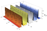
(a)     (b)

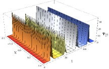
Figure 1: Profiles of the non-Wick-type solution (41): (a) $\dot{B}_{t}=i\cos(0.1t)$ and (b) $\dot{B}_{t}=0$, under $p(t)=-1$, $q(t)=0.2$, $c=-0.01$, $\alpha(t)=-1.5i\cos(0.2t)$, $\lambda(t)=i\cos(0.2t)$.

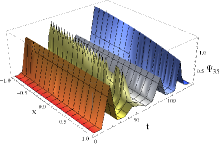
(a)     (b)

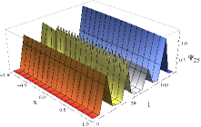
Figure 2: Profiles of the non-Wick-type solution (42): (a) $\dot{B}(t)=0.25i(\cos(0.1t)+1.5\sin(0.5t))$; (b) $\dot{B}(t)=0$, under $p(t)=-1$, $q(t)=0.2$, $c=-0.01$, $\alpha(t)=-1.5i\cos(0.2t)$, $\lambda(t)=i\cos(0.2t)$.

In particular, Fig. 1 and 2 are plotted for time-dependent coefficients $\alpha(t),\lambda(t)$, without white noise effect and with white noise effect, respectively. In Fig. 1, with white noise functional, the white noise effect is generated in the part (a) as time changes, and without white noise functional, the noise is disappearing as time increases in the part (b). Fig. 2 performs the behaviors of the solitons-like traveling wave solution (42) or the white noise functionals.

3 Wick-type stochastic fractional RLW-Burgers equation

The Caputo fractional derivative of order $0<\alpha<1$ is defined as follows [39]:

$${}^{c}D_{t}^{\alpha}f(t)=\frac{1}{\Gamma(1-\alpha)}\frac{\partial}{\partial\tau}\int_{0}^{t}\frac{f(\tau)}{(t-\tau)^{\alpha}}d\tau.$$ (43)

Some useful properties for the Caputo regularized partial derivative are:

$${}^{c}D_{t}^{\alpha}t^{r}=\frac{\Gamma(1+r)}{\Gamma(1+r-\alpha)}t^{r-\alpha},$$ (44)

$${}^{c}D_{t}^{\alpha}(f(t)g(t))=g(t){}^{c}D_{t}^{\alpha}f(t)+f(t){}^{c}D_{t}^{\alpha}g(t),$$ (45)

$${}^{c}D_{t}^{\alpha}f[g(t)]=f^{\prime}[g(t)]{}^{c}D_{t}^{\alpha}g(t).$$ (46)

In this section, we present the main steps of the mathematical computation with the Caputo fractional derivative for obtaining exact solutions of fractional NPDEs.

3.1 Mathematical computation scheme with fractional order

Consider the fractional improved Riccati equations with parameter functions as follows:

$$\cases{D_{\xi}^{\alpha}\Psi(\xi)=\lambda(t)\Psi(\xi),\cr D_{\xi}^{\alpha}\Phi(\xi)=\lambda(t)\Psi(\xi)+\mu(t)\Phi(\xi),}$$ (47)

where $\lambda(t)$ and $\mu(t)$ denote arbitrary integrable functions, $D_{\xi}^{\alpha}\Psi(\xi)$ and $D_{\xi}^{\alpha}\Phi(\xi)$ denote the Caputo fractional derivative of fractional-order $\alpha$ for $\Psi(\xi)$ and $\Phi(\xi)$, and ${}^{c}D_{\xi}^{\alpha}=D_{\xi}^{\alpha}$ for using a simple notation. In order to obtain the solutions for Eq. (47), we consider $\Psi(\xi)=\psi(\eta)$ and $\Phi(\xi)=\phi(\eta)$ with a nonlinear fractional complex transformation $\eta=\xi^{\alpha}/\Gamma(1+\alpha)$. By using Eq. (44) and Eq. (46), that is, $D_{\xi}^{\alpha}\Psi(\xi)=D_{\xi}^{\alpha}\psi(\eta)=\psi^{\prime}(\eta)D_{\xi}^{\alpha}\eta=\psi^{\prime}(\eta)$ and $D_{\xi}^{\alpha}\Phi(\xi)=D_{\xi}^{\alpha}\phi(\eta)=\phi^{\prime}(z)D_{\xi}^{\alpha}\eta=\phi^{\prime}(\eta)$, the fractional improved Riccati equations (47) can be transformed to the improved Riccati equation in the following form:

$$\cases{\psi^{\prime}(\eta)=\lambda(t)\mbox{~{}}\psi(\eta),\cr\phi^{\prime}(\eta)=\lambda(t)\mbox{~{}}\psi(\eta)+\mu(t)\phi(\eta).}$$ (48)

From the general solutions of Eq. (48), we construct the ans$\ddot{{\rm a}}$tz in the following form:

$$\left\{\frac{\psi(\eta)}{\phi(\eta)}\right\}=\frac{\lambda(t)-\mu(t)}{\lambda(t)-\mu(t)\exp\{-(\lambda(t)-\mu(t))\eta\}},$$ (49)

and by substituting the nonlinear fractional transformation $\eta=\xi^{\alpha}/\Gamma(1+\alpha)$, the ans$\ddot{{\rm a}}$tz (49) can be rewritten in the following form:

$$\left\{\frac{\Psi(\xi)}{\Phi(\xi)}\right\}=\frac{\lambda(t)-\mu(t)}{\lambda(t)-\mu(t)\exp\{-(\lambda(t)-\mu(t))\frac{\xi^{\alpha}}{\Gamma(1+\alpha)}\}}.$$ (50)

Suppose that the fractional Wick-type stochastic NPDE with the independent variables $t,x_{1},x_{2},\ldots,x_{n}$, is given by

$$\mathcal{P}^{\diamondsuit}\left(u,D_{t}^{\diamondsuit\alpha}u,D_{x_{1}}^{\diamondsuit\alpha}u,D_{x_{2}}^{\diamondsuit\alpha}u,\ldots,D_{t}^{\diamondsuit 2\alpha}u,D_{x_{1}}^{\diamondsuit 2\alpha}u,D_{x_{2}}^{\diamondsuit 2\alpha}u,\ldots\right)=0,$$ (51)

where $D_{t}^{\diamondsuit\alpha}u,D_{x_{1}}^{\diamondsuit\alpha}u,D_{x_{2}}^{\diamondsuit\alpha}u,\ldots,D_{t}^{\diamondsuit 2\alpha}u,D_{x_{1}}^{\diamondsuit 2\alpha}u,D_{x_{2}}^{\diamondsuit 2\alpha}u,\ldots$, are the Caputo fractional derivatives of $u$ in the Wick-type sense with respect to $t,x_{1},x_{2},\ldots,x_{n}$ and $u=u(t,x_{1},x_{2},\ldots,x_{n})$. $\mathcal{P}$ is a polynomial in $u$ and its various partial fractional derivatives.

Step 1. Suppose that traveling wave transformation is given by

$$\cases{u(t,x_{1},x_{2},\ldots,x_{n})=U(\zeta),\cr\zeta=\int_{0}^{T}c(s)ds+\frac{k_{1}x_{1}^{\alpha}}{\Gamma(1+\alpha)}+\frac{k_{2}x_{2}^{\alpha}}{\Gamma(1+\alpha)}+\cdots+\frac{k_{n}x_{n}^{\alpha}}{\Gamma(1+\alpha)},T=\frac{t^{\alpha}}{\Gamma(1+\alpha)}}$$ (52)

where $k_{1},k_{2},\ldots,k_{n}$ represent nonzero constants and $c(t)$ is an integrable function of $t$. Then, by the property (46) of the Caputo fractional derivative and by taking $u=\tilde{U}(\zeta)$, $D_{t}^{\alpha}u=c(T)\tilde{U}_{\zeta}$, $D_{x_{1}}^{\alpha}u=k_{1}\tilde{U}_{\zeta}$, $D_{x_{2}}^{\alpha}u=k_{2}\tilde{U}_{\zeta}$, $\ldots$, $D_{t}^{2\alpha}u=c^{2}(T)\tilde{U}_{\zeta\zeta}$, $D_{x_{1}}^{2\alpha}u=k_{1}^{2}\tilde{U}_{\zeta\zeta}$, $D_{x_{2}}^{2\alpha}u=k_{2}^{2}\tilde{U}_{\zeta\zeta}$, $\ldots$, the Eq. (51) can be reduced into the following fractional ordinary differential equation with respect to traveling wave variable $\zeta$:

$$\tilde{\mathcal{P}}(\tilde{U},c\tilde{U}^{\prime},k_{1}\tilde{U}^{\prime},k_{2}\tilde{U}^{\prime}\ldots,c^{2}\tilde{U}^{\prime\prime},k_{1}^{2}\tilde{U}^{\prime\prime},k_{2}^{2}\tilde{U}^{\prime\prime}\ldots,z)=0,$$ (53)

where $c=c(T),\tilde{U}^{\prime}=\tilde{U}_{\zeta},\tilde{U}^{\prime\prime}=\tilde{U}_{\zeta\zeta},\ldots$, and $\tilde{U}=\mathcal{H}(U)$ is the Hermite transform of $U$ and $z=(z_{1},z_{2},\ldots)$ is a vector of all sequences of complex numbers. Suppose that we can find the solution $u=\tilde{U}(t,x,z)$ of Eq. (53) for $z\in\mathbb{K}_{m}(n)$, where $\mathbb{K}_{m}(n)=\{(z_{1},z_{2},\ldots)\in\mathbb{C}^{n}\mbox{~{}}{\rm and}\mbox{~{}}\sum_{\alpha}|z^{\alpha}|^{2}(2N)^{m\alpha}<n^{2}\}$ for some integers $m,n$, $x=(x_{1},x_{2},\ldots,x_{n})$ and $z=(z_{1},z_{2},\ldots,z_{n})$.

Step 2. Suppose that the solution of Eq. (53) can be expressed by a polynomial in $\left\{\psi(\zeta)/\phi(\zeta)\right\}$ as given below:

$$\tilde{U}(\zeta)=\sum_{i=0}^{m}A_{i}(t)\left\{\frac{\psi(\zeta)}{\phi(\zeta)}\right\}^{i},$$ (54)

where $\left\{\psi(\zeta)/\phi(\zeta)\right\}$ is the ans$\ddot{{\rm a}}$tz (49) and $\{A_{i}(t)\}_{i=0}^{m}$ are unknown coefficients to be computed later, $A_{m}(t)\neq 0$. The pole-order $m$ can be determined by considering the homogeneous balancing principle between the highest order linear term and the highest order nonlinear term that occurs in Eq. (53).

Step 3. Substituting the solution (54) into Eq. (53), collecting all terms with the same order of $\left\{\psi(\zeta)/\phi(\zeta)\right\}$ together, the left-hand side of Eq. (53) changed into another polynomial in $\left\{\psi(\zeta)/\phi(\zeta)\right\}$. Equating each coefficient of this resulting polynomial to zero, we get a set of algebraic equations for coefficients $\left\{A_{i}(t)\right\}_{i=0}^{m},\left\{k_{i}\right\}_{i=1}^{n}$ and $c(t)$.

Step 4. Solving the resulting set of obtained algebraic equations in Step 3 and combining the solution (54), the traveling wave transformation (52) and the fractional ans$\ddot{\rm a}$tz (50), under certain conditions, we can take the inverse Hermite transform $\tilde{U}=\mathcal{H}^{-1}(u)\in(\mathcal{S})_{-1}$ and hence we obtain the Wick-type solution $u$ of the original fractional Wick-type stochastic NPDE (51) [38].

3.2 Wick-type fractional exact traveling wave solutions of equation (4)

Now, by applying the Hermite transform, the fractional Wick-type stochastic RLW-Burgers equation is converted into a deterministic fractional NPDE, which is expressed in the following form:

$$\frac{\partial^{\alpha}\tilde{V}}{\partial t^{\alpha}}+\tilde{P}(t,z)\frac{\partial^{\alpha}\tilde{V}}{\partial x^{\alpha}}+\tilde{Q}(t,z)\tilde{V}\frac{\partial^{\alpha}\tilde{V}}{\partial x^{\alpha}}+\tilde{R}(t,z)\frac{\partial^{2\alpha}\tilde{V}}{\partial x^{2\alpha}}+\tilde{S}(t,z)\frac{\partial^{3\alpha}\tilde{V}}{\partial t^{\alpha}\partial x^{2\alpha}}=0,$$ (55)

where $z=(z_{1},z_{2},\ldots)\in\mathbb{C}^{n}$ is a vector parameter. To derive exact traveling wave solutions of Eq. (55), we consider the solution form $\tilde{V}=\tilde{V}(x,t,z)=\textsf{y}(\zeta(x,t,z))$ with the traveling wave variable

$$\zeta(x,t,z)=kX+\int_{0}^{T}c(s,z)ds,$$ (56)

where $X=\frac{x^{\alpha}}{\Gamma(1+\alpha)},T=\frac{t^{\alpha}}{\Gamma(1+\alpha)}$, $k$ is a nonzero constant and $c(s,z)$ is a nonzero function of the indicated variables to be calculated later. By using the traveling wave variable (56), Eq. (55) can be converted into the form

$$(c(T,z)+kp(t,z))\textsf{y}^{\prime}+kq(t,z)\textsf{y}\textsf{y}^{\prime}+k^{2}r(t,z)\textsf{y}^{\prime\prime}+kc(T,z)s(t,z)\textsf{y}^{\prime\prime\prime}=0,$$ (57)

where $\textsf{y}^{\prime}=\frac{d\tilde{V}}{d\zeta},\textsf{y}^{\prime\prime}=\frac{d^{2}\tilde{V}}{d\zeta^{2}},\textsf{y}^{\prime\prime\prime}=\frac{d^{3}\tilde{V}}{d\zeta^{3}}$ and $p(t,z)=\tilde{P}(t,z),q(t,z)=\tilde{Q}(t,z),r(t,z)=\tilde{R}(t,z),s(t,z)=\tilde{S}(t,z).$ Integrating Eq. (57) with respect to $\zeta$ once, we can get

$$(c(T,z)+kp(t,z))\textsf{y}+\frac{1}{2}kq(t,z)\textsf{y}^{2}+k^{2}r(t,z)\textsf{y}^{\prime}+k^{2}c(T,z)s(t,z)\textsf{y}^{\prime\prime}=0.$$ (58)

Here the arbitrary integral constant is assumed to be zero.

To determine the pole-order $m$ of the exact traveling wave solution of Eq. (58), by balancing the highest order linear term $\textsf{y}^{\prime\prime}$ and the highest order nonlinear term $\textsf{y}^{2}$ in Eq. (58), we obtain $N+2=2N$, which gives $N=2$. Now, we assume that the second-order pole exact traveling wave solution of Eq. (58) can be expressed by the following form:

$$\textsf{y}(\zeta)=\sum_{i=0}^{2}A_{i}(t,z)\left\{\frac{\psi(\zeta)}{\phi(\zeta)}\right\}^{i}.$$ (59)

Substituting the solution (59) into Eq. (58), collecting all the terms with the same power of $\{\psi(\zeta)/\phi(\zeta)\}$ together and equating each coefficient of this polynomial to zero, we obtain a set of algebraic equations for $A_{0}(t,z),A_{1}(t,z),A_{2}(t,z)$ and $c(t,z)$. Further, by solving the algebraic equations and substituting the coefficients of nontrivial solutions and the traveling wave variable (56) into Eq. (59), we obtain six exact traveling wave solutions of Eq. (55). Let $\tau_{\alpha}=[\tau\Gamma(1+\alpha)]^{1/\alpha}$, $B_{1}(t,z)=r(t,z)-s(t,z)\mu(t,z)$, $B_{2}(t,z)=r(t,z)-2s(t,z)\mu(t,z)$, $C_{1}(t,z)=r(t,z)-6s(t,z)\mu(t,z)$, $C_{2}(t,z)=r(t,z)-5s(t,z)\mu(t,z)$, $D_{1}(t,z)=r(t,z)+4s(t,z)\mu(t,z)$, $D_{2}(t,z)=r(t,z)-2s(t,z)\mu(t,z)$, and $k$ be a nonzero constant.

The first exact traveling wave solution with a relation $\lambda(t,z)=(r(t,z)-s(t,z)\mu(t,z))/s(t,z)$ is expressed by the form

$$\tilde{V}_{1}(x,t,z)=\frac{12kB_{1}(t,z)B_{2}^{2}(t,z)}{q(t,z)s(t,z)\left[B_{1}(t,z)-s(t,z)\mu(t,z)\exp\{-\frac{B_{2}(t,z)}{s(t,z)}\zeta_{1}(x,t,z)\}\right]}\mbox{~{}~{}~{}~{}~{}}$$ (60)

$$-\frac{12kB_{1}^{2}(t,z)B_{2}(t,z)}{q(t,z)s(t,z)\left[B_{1}(t,z)-s(t,z)\mu(t,z)\exp\{-\frac{B_{2}(t,z)}{s(t,z)}\zeta_{1}(x,t,z)\}\right]^{2}},$$ (61)

where $\zeta_{1}(x,t,z)=\frac{kx^{\alpha}}{\Gamma(1+\alpha)}+\int_{0}^{\frac{t^{\alpha}}{\Gamma(1+\alpha)}}c(\tau,z)d\tau$ and

$$c(\tau,z)=-k(4k\mu^{2}(\tau_{\alpha},z)s(\tau_{\alpha},z)-4kr(\tau_{\alpha},z)\mu(\tau_{\alpha},z)+p(\tau_{\alpha},z)+kr^{2}(\tau_{\alpha},z)/s(\tau_{\alpha},z)).$$

The second exact traveling wave solution with relation $\lambda(t,z)=-(r(t,z)-6s(t,z)\mu(t,z))/s(t,z)$ is given by

$$\tilde{V}_{2}(x,t,z)=-\frac{3kC_{1}^{2}(t,z)C_{2}(t,z)}{4q(t,z)s(t,z)\left[C_{1}(t,z)+s(t,z)\mu(t,z)\exp\{-\frac{C_{2}(t,z)}{s(t,z)}\zeta_{2}(x,t,z)\}\right]^{2}},$$ (62)

where $\zeta_{2}(x,t,z)=\frac{kx^{\alpha}}{\Gamma(1+\alpha)}+\int_{0}^{\frac{t^{\alpha}}{\Gamma(1+\alpha)}}c(\tau,z)d\tau$ and

$$c(\tau,z)=k(12k\mu^{2}(\tau_{\alpha},z)s(\tau_{\alpha},z)-12kr(\tau_{\alpha},z)\mu(\tau_{\alpha},z)-8p(\tau_{\alpha},z)+3kr^{2}(\tau_{\alpha},z)/s(\tau_{\alpha},z))/8.$$

The third exact traveling wave solution with relation $\lambda(t,z)=(r(t,z)+4s(t,z)\mu(t,z))/(6s(t,z))$ can be expressed by

$$\tilde{V}_{3}(x,t,z)=\frac{2kD_{1}(t,z)D_{2}^{2}(t,z)}{q(t,z)s(t,z)\left[D_{1}(t,z)-6s(t,z)\mu(t,z)\exp\{-\frac{D_{2}(t,z)}{6s(t,z)}\zeta_{3}(x,t,z)\}\right]}\mbox{~{}~{}~{}~{}~{}}$$ (63)

$$-\frac{kD_{1}^{2}(t,z)D_{2}(t,z)}{3q(t,z)s(t,z)\left[D_{1}(t,z)-6s(t,z)\mu(t,z)\exp\{-\frac{D_{2}(t,z)}{6s(t,z)}\zeta_{3}(x,t,z)\}\right]^{2}},$$ (64)

where $\zeta_{3}(x,t,z)=\frac{kx^{\alpha}}{\Gamma(1+\alpha)}+\int_{0}^{\frac{t^{\alpha}}{\Gamma(1+\alpha)}}c(\tau,z)d\tau$, $k$ an arbitrary constant, and

$$c(\tau,z)=-k(4k\mu^{2}(\tau_{\alpha},z)s(\tau_{\alpha},z)-4kr(\tau_{\alpha},z)\mu(\tau_{\alpha},z)+6p(\tau_{\alpha},z)+kr^{2}(\tau_{\alpha},z)/s(\tau_{\alpha},z))/6.$$

The fourth exact traveling wave solution with relation $\lambda(t,z)=(r(t,z)-s(t,z)\mu(t,z))/s(t,z)$ is expressed by

$$\tilde{V}_{4}(x,t,z)=-\frac{2kB_{2}^{2}(t,z)}{s(t,z)\mu(t,z)}\frac{12kB_{1}(t,z)B_{2}^{2}(t,z)}{q(t,z)s(t,z)\left[B_{1}(t,z)-s(t,z)\mu(t,z)\exp\{-\frac{B_{2}(t,z)}{s(t,z)}\zeta_{4}(x,t,z)\}\right]}\mbox{~{}}$$ (65)

$$-\frac{12kB_{1}^{2}(t,z)B_{2}(t,z)}{q(t,z)s(t,z)\left[B_{1}(t,z)-s(t,z)\mu(t,z)\exp\{-\frac{B_{2}(t,z)}{s(t,z)}\zeta_{4}(x,t,z)\}\right]^{2}},$$ (66)

where $\zeta_{4}(x,t,z)=\frac{kx^{\alpha}}{\Gamma(1+\alpha)}+\int_{0}^{\frac{t^{\alpha}}{\Gamma(1+\alpha)}}c(\tau,z)d\tau$ and

$$c(\tau,z)=k(4k\mu^{2}(\tau_{\alpha},z)s(\tau_{\alpha},z)-4kr(\tau_{\alpha},z)\mu(\tau_{\alpha},z)-p(\tau_{\alpha},z)+kr^{2}(\tau_{\alpha},z)/s(\tau_{\alpha},z)).$$

The fifth exact traveling wave solution with relation $\lambda(t,z)=-(r(t,z)-6s(t,z)\mu(t,z))/s(t,z)$ is given by

$$\tilde{V}_{5}(x,t,z)=\frac{3kB_{2}^{2}(t,z)}{4q(t,z)s(t,z)}-\frac{3kC_{1}^{2}(t,z)C_{2}(t,z)}{4q(t,z)s(t,z)\left[C_{1}(t,z)+s(t,z)\mu(t,z)\exp\{-\frac{C_{2}(t,z)}{s(t,z)}\zeta_{5}(x,t,z)\}\right]^{2}},$$ (67)

where $\zeta_{5}(x,t,z)=\frac{kx^{\alpha}}{\Gamma(1+\alpha)}+\int_{0}^{\frac{t^{\alpha}}{\Gamma(1+\alpha)}}c(\tau,z)d\tau$ and

$$c(\tau,z)=-k(12k\mu^{2}(\tau_{\alpha},z)s(\tau_{\alpha},z)-12kr(\tau_{\alpha},z)\mu(\tau_{\alpha},z)+8p(\tau_{\alpha},z)+3kr^{2}(\tau_{\alpha},z)/s(\tau_{\alpha},z))/8.$$

Finally, the sixth exact traveling wave solution with relation $\lambda(t,z)=(r(t,z)+4s(t,z)\mu(t,z))/(6s(t,z))$ is given by

$$\tilde{V}_{6}(x,t,z)=\frac{2kD_{1}(t,z)D_{2}^{2}(t,z)}{q(t,z)s(t,z)\left[D_{1}(t,z)-6s(t,z)\mu(t,z)\exp\{-\frac{D_{2}(t,z)}{6s(t,z)}\zeta_{6}(x,t,z)\}\right]}\mbox{~{}~{}~{}~{}~{}}$$ (68)

$$-\frac{kD_{1}^{2}(t,z)D_{2}(t,z)}{3q(t,z)s(t,z)\left[D_{1}(t,z)-6s(t,z)\mu(t,z)\exp\{-\frac{D_{2}(t,z)}{6s(t,z)}\zeta_{6}(x,t,z)\}\right]^{2}},$$ (69)

where $\zeta_{6}(x,t,z)=\frac{kx^{\alpha}}{\Gamma(1+\alpha)}+\int_{0}^{\frac{t^{\alpha}}{\Gamma(1+\alpha)}}c(\tau,z)d\tau$ and

$$c(\tau,z)=k(4k\mu^{2}(\tau_{\alpha},z)s(\tau_{\alpha},z)-4kr(\tau_{\alpha},z)\mu(\tau_{\alpha},z)-6p(\tau_{\alpha},z)+kr^{2}(\tau_{\alpha},z)/s(\tau_{\alpha},z))/6.$$

In order to obtain the white noise functional solutions of Eq. (4), we need to use the inverse Hermite transform and Theorem 4.1.1 in [38]. Then we can obtain the Wick-type exact traveling wave solutions as the white noise functional solutions of Eq. (4) based on the solutions (61)–(69) in the following form:

$$V_{1}(x,t)=\frac{12kB_{1}(t)\diamondsuit B_{2}^{\diamondsuit 2}(t)}{Q(t)\diamondsuit S(t)\diamondsuit\left[B_{1}(t)-S(t)\diamondsuit\mu(t)\diamondsuit\exp^{\diamondsuit}\{-\frac{B_{2}(t)}{S(t)}\diamondsuit\Xi_{1}(x,t)\}\right]}\mbox{~{}}$$ (70)

$$-\frac{12kB_{1}^{\diamondsuit 2}(t)\diamondsuit B_{2}(t)}{Q(t)\diamondsuit S(t)\diamondsuit\left[B_{1}(t)-S(t)\diamondsuit\mu(t)\diamondsuit\exp^{\diamondsuit}\{-\frac{B_{2}(t)}{S(t)}\diamondsuit\Xi_{1}(x,t)\}\right]^{\diamondsuit 2}},$$ (71)

where $\Xi_{1}(x,t)=\frac{kx^{\alpha}}{\Gamma(1+\alpha)}+\int_{0}^{\frac{t^{\alpha}}{\Gamma(1+\alpha)}}c(\tau)d\tau$ and

$$c(\tau)=-k(4k\mu^{\diamondsuit 2}(\tau_{\alpha})\diamondsuit S(\tau_{\alpha})-4kR(\tau_{\alpha})\diamondsuit\mu(\tau_{\alpha})+P(\tau_{\alpha})+kR^{\diamondsuit 2}(\tau_{\alpha})/S(\tau_{\alpha})),$$

$$V_{2}(x,t)=-\frac{3kC_{1}^{\diamondsuit 2}(t)\diamondsuit C_{2}(t)}{4Q(t)\diamondsuit S(t)\diamondsuit\left[C_{1}(t)+S(t)\diamondsuit\mu(t)\diamondsuit\exp^{\diamondsuit}\{-\frac{C_{2}(t)}{S(t)}\diamondsuit\Xi_{2}(x,t)\}\right]^{\diamondsuit 2}},$$ (72)

where $\Xi_{2}(x,t)=\frac{kx^{\alpha}}{\Gamma(1+\alpha)}+\int_{0}^{\frac{t^{\alpha}}{\Gamma(1+\alpha)}}c(\tau)d\tau$ and

$$c(\tau)=k(12k\mu^{\diamondsuit 2}(\tau_{\alpha})\diamondsuit S(\tau_{\alpha})-12kR(\tau_{\alpha})\diamondsuit\mu(\tau_{\alpha})-8P(\tau_{\alpha})+3kR^{\diamondsuit 2}(\tau_{\alpha})/S(\tau_{\alpha}))/8,$$

$$V_{3}(x,t)=\frac{2kD_{1}(t)\diamondsuit D_{2}^{\diamondsuit 2}(t)}{Q(t)\diamondsuit S(t)\diamondsuit\left[D_{1}(t)-6S(t)\diamondsuit\mu(t)\diamondsuit\exp^{\diamondsuit}\{-\frac{D_{2}(t)}{6S(t)}\diamondsuit\Xi_{3}(x,t)\}\right]}\mbox{~{}~{}~{}~{}}$$ (73)

$$-\frac{kD_{1}^{\diamondsuit 2}(t)\diamondsuit D_{2}(t)}{3Q(t)\diamondsuit S(t)\diamondsuit\left[D_{1}(t)-6S(t)\diamondsuit\mu(t)\diamondsuit\exp^{\diamondsuit}\{-\frac{D_{2}(t)}{6S(t)}\diamondsuit\Xi_{3}(x,t)\}\right]^{\diamondsuit 2}},$$ (74)

where $\Xi_{3}(x,t)=\frac{kx^{\alpha}}{\Gamma(1+\alpha)}+\int_{0}^{\frac{t^{\alpha}}{\Gamma(1+\alpha)}}c(\tau)d\tau$ and

$$c(\tau)=-k(4k\mu^{2}(\tau_{\alpha})\diamondsuit S(\tau_{\alpha})-4kR(\tau_{\alpha})\diamondsuit\mu(\tau_{\alpha})+6P(\tau_{\alpha})+kR^{\diamondsuit 2}(\tau_{\alpha})/S(\tau_{\alpha}))/6,$$

$$V_{4}(x,t)=-\frac{2kB_{2}^{\diamondsuit 2}(t)}{S(t)\diamondsuit Q(t)}+\frac{12kB_{1}(t)\diamondsuit B_{2}^{\diamondsuit 2}(t)}{Q(t)\diamondsuit S(t)\diamondsuit\left[B_{1}(t)-S(t)\diamondsuit\mu(t)\diamondsuit\exp^{\diamondsuit}\{-\frac{B_{2}(t)}{S(t)}\diamondsuit\Xi_{4}(x,t)\}\right]}\mbox{~{}}$$ (75)

$$-\frac{12kB_{1}^{\diamondsuit 2}(t)\diamondsuit B_{2}(t)}{Q(t)\diamondsuit S(t)\diamondsuit\left[B_{1}(t)-S(t)\diamondsuit\mu(t)\diamondsuit\exp^{\diamondsuit}\{-\frac{B_{2}(t)}{S(t)}\diamondsuit\Xi_{4}(x,t)\}\right]^{\diamondsuit 2}},$$ (76)

where $\Xi_{4}(x,t)=\frac{kx^{\alpha}}{\Gamma(1+\alpha)}+\int_{0}^{\frac{t^{\alpha}}{\Gamma(1+\alpha)}}c(\tau)d\tau$ and

$$c(\tau)=-k(4k\mu^{\diamondsuit 2}(\tau_{\alpha})\diamondsuit S(\tau_{\alpha})-4kR(\tau_{\alpha})\diamondsuit\mu(\tau_{\alpha})-P(\tau_{\alpha})+kR^{\diamondsuit 2}(\tau_{\alpha})/S(\tau_{\alpha})),$$

$$V_{5}(x,t)=\frac{3kB_{2}^{\diamondsuit 2}(t)}{4S(t)\diamondsuit Q(t)}-\frac{3kC_{1}^{\diamondsuit 2}(t)\diamondsuit C_{2}(t)}{4Q(t)\diamondsuit S(t)\diamondsuit\left[C_{1}(t)+S(t)\diamondsuit\mu(t)\diamondsuit\exp^{\diamondsuit}\{-\frac{C_{2}(t)}{S(t)}\diamondsuit\Xi_{5}(x,t)\}\right]^{\diamondsuit 2}},$$ (77)

where $\Xi_{5}(x,t)=\frac{kx^{\alpha}}{\Gamma(1+\alpha)}+\int_{0}^{\frac{t^{\alpha}}{\Gamma(1+\alpha)}}c(\tau)d\tau$ and

$$c(\tau)=-k(12k\mu^{\diamondsuit 2}(\tau_{\alpha})\diamondsuit S(\tau_{\alpha})-12kR(\tau_{\alpha})\diamondsuit\mu(\tau_{\alpha})+8P(\tau_{\alpha})+3kR^{\diamondsuit 2}(\tau_{\alpha})/S(\tau_{\alpha}))/8,$$

and

$$V_{6}(x,t)=-\frac{kB_{2}^{\diamondsuit 2}(t)}{3S(t)\diamondsuit Q(t)}+\frac{2kD_{1}(t)\diamondsuit D_{2}^{\diamondsuit 2}(t)}{Q(t)\diamondsuit S(t)\diamondsuit\left[D_{1}(t)-6S(t)\diamondsuit\mu(t)\diamondsuit\exp^{\diamondsuit}\{-\frac{D_{2}(t)}{6S(t)}\diamondsuit\Xi_{6}(x,t)\}\right]}\mbox{~{}}$$ (78)

$$-\frac{kD_{1}^{\diamondsuit 2}(t)\diamondsuit D_{2}(t)}{3Q(t)\diamondsuit S(t)\diamondsuit\left[D_{1}(t)-6S(t)\diamondsuit\mu(t)\diamondsuit\exp^{\diamondsuit}\{-\frac{D_{2}(t)}{6S(t)}\diamondsuit\Xi_{6}(x,t)\}\right]^{\diamondsuit 2}},$$ (79)

where $\Xi_{6}(x,t)=\frac{kx^{\alpha}}{\Gamma(1+\alpha)}+\int_{0}^{\frac{t^{\alpha}}{\Gamma(1+\alpha)}}c(\tau)d\tau$ and

$$c(\tau)=k(4k\mu^{\diamondsuit 2}(\tau_{\alpha})\diamondsuit S(\tau_{\alpha})-4kR(\tau_{\alpha})\diamondsuit\mu(\tau_{\alpha})-6P(\tau_{\alpha})+kR^{\diamondsuit 2}(\tau_{\alpha})/S(\tau_{\alpha}))/6.$$

Here, $\tau_{\alpha}=[\tau\Gamma(1+\alpha)]^{1/\alpha}$, $B_{1}(t)=R(t)-S(t)\diamondsuit\mu(t)$, $B_{2}(t)=R(t)-2S(t)\diamondsuit\mu(t)$, $C_{1}(t)=R(t)-6S(t)\diamondsuit\mu(t)$, $C_{2}(t)=R(t)-5S(t)\diamondsuit\mu(t)$, $D_{1}(t)=R(t)+4S(t)\diamondsuit\mu(t)$, $D_{2}(t)=R(t)-2S(t)\diamondsuit\mu(t)$, and $k$ is a nonzero constant.

Note that the obtained solutions contain arbitrary functions, which reveal the physical quantities $V_{i}$, $i=1,2,\ldots,6$. These solutions possess rich structures and can be used to discuss some particular physical situations through the choice of the arbitrary functions. Note also that for different forms of $P(t)$, $Q(t)$, $R(t)$ and $S(t)$, we can get white noise functional solutions of exponential type of Eq. (4) from the obtained solutions (71)–(79).

Example 3.1

Assume $R(t)=0$ and take $P(t)=f_{1}(t)+c_{1}W(t)$, $Q(t)=f_{2}(t)+c_{2}W(t)$, $S(t)=f_{4}(t)+c_{4}W(t)$, where $c_{i}$, $i=1,2,4$, are arbitrary constants and $f_{i}(t)$, $i=1,2,4$, are bounded functions on $\mathbb{R}^{+}$, where $W(t)$ is the Gaussian white noise, i.e., $W(t)=\dot{B}(t)=dB(t)/dt$, $B(t)$ is a Brownian motion. Also we have the Hermite transform $P(t,z)=f_{1}(t)+c_{1}\tilde{W}(t,z)$, $Q(t,z)=f_{2}(t)+c_{2}\tilde{W}(t,z)$, $S(t,z)=f_{4}(t)+c_{4}\tilde{W}(t,z)$, where $\tilde{W}(t,z)=\sum_{i=1}^{\infty}\int_{0}^{t}\zeta_{i}(s)dsz_{i}$, $z=(z_{1},z_{2},\ldots)\in\mathbb{C}^{n}$ is a parameter vector and $\zeta_{i}(s)$ is defined in [38]. By the definition of $\tilde{W}(t,z)$, the Wick-type exact traveling wave solutions (71)–(79) give the white noise functional solutions of Eq. (4) as follows:

$$V_{1}(x,t)=\frac{48k(f_{4}(t)+c_{4}W(t))\mu^{2}(t)}{(f_{2}(t)+c_{2}W(t))\left[1+\exp\{2\mu(t)\Xi_{1}(x,t)\}\right]}\mbox{~{}}-\frac{48k(f_{4}(t)+c_{4}W(t))\mu^{2}(t)}{(f_{2}(t)+c_{2}W(t))\left[1+\exp\{2\mu(t)\Xi_{1}(x,t)\}\right]^{2}},$$ (80)

where $\Xi_{1}(x,t)=\frac{kx^{\alpha}}{\Gamma(1+\alpha)}+\int_{0}^{\frac{t^{\alpha}}{\Gamma(1+\alpha)}}c(\tau)d\tau$, $c(\tau)=-k(4k\mu^{2}(\tau_{\alpha})(f_{4}(\tau_{\alpha})+c_{4}W(t))+(f_{1}(\tau_{\alpha})+c_{1}W(t)))$ and $\tau_{\alpha}=[\tau\Gamma(1+\alpha)]^{1/\alpha}$,

$$V_{2}(x,t)=-\frac{675k(f_{4}(t)+c_{4}W(t))\mu^{2}(t)}{(f_{2}(t)+c_{2}W(t))\left[6-\exp\{5\mu(t)\Xi_{2}(x,t)\}\right]^{2}},$$ (81)

where $\Xi_{2}(x,t)=\frac{kx^{\alpha}}{\Gamma(1+\alpha)}+\int_{0}^{\frac{t^{\alpha}}{\Gamma(1+\alpha)}}c(\tau)d\tau$, $c(\tau)=-(3k^{2}\mu^{2}(\tau_{\alpha})(f_{4}(\tau_{\alpha})+c_{4}W(t))-2k(f_{1}(\tau_{\alpha})+c_{1}W(t)))/2$ and $\tau_{\alpha}=[\tau\Gamma(1+\alpha)]^{1/\alpha}$,

$$V_{3}(x,t)=\frac{16k(f_{4}(t)+c_{4}W(t))\mu^{2}(t)}{(f_{2}(t)+c_{2}W(t))\left[2-3\exp\{\mu(t)\Xi_{3}(x,t)/3\}\right]}\mbox{~{}}-\frac{16k(f_{4}(t)+c_{4}W(t))\mu^{2}(t)}{3(f_{2}(t)+c_{2}W(t))\left[2-3\exp\{\mu(t)\Xi_{3}(x,t)/3\}\right]^{2}},$$ (82)

where $\Xi_{3}(x,t)=\frac{kx^{\alpha}}{\Gamma(1+\alpha)}+\int_{0}^{\frac{t^{\alpha}}{\Gamma(1+\alpha)}}c(\tau)d\tau$, $c(\tau)=-(4k^{2}\mu^{2}(\tau_{\alpha})(f_{4}(\tau_{\alpha})+c_{4}W(t))+6k(f_{1}(\tau_{\alpha})+c_{1}W(t)))/6$ and $\tau_{\alpha}=[\tau\Gamma(1+\alpha)]^{1/\alpha}$,

$$V_{4}(x,t)=-\frac{8k\mu^{2}(t)(f_{4}(t)+c_{4}W(t))}{f_{2}(t)+c_{2}W(t)}+\frac{48k(f_{4}(t)+c_{4}W(t))\mu^{2}(t)}{(f_{2}(t)+c_{2}W(t))\left[1+\exp\{2\mu(t)\Xi_{4}(x,t)\}\right]}\mbox{~{}}$$ (83)

$$-\frac{48k(f_{4}(t)+c_{4}W(t))\mu^{2}(t)}{(f_{2}(t)+c_{2}W(t))\left[1+\exp\{2\mu(t)\Xi_{4}(x,t)\}\right]^{2}},$$ (84)

where $\Xi_{4}(x,t)=\frac{kx^{\alpha}}{\Gamma(1+\alpha)}+\int_{0}^{\frac{t^{\alpha}}{\Gamma(1+\alpha)}}c(\tau)d\tau$, $c(\tau)=k(4k\mu^{2}(\tau_{\alpha})(f_{4}(\tau_{\alpha})+c_{4}W(t))+(f_{1}(\tau_{\alpha})+c_{1}W(t)))$, and $\tau_{\alpha}=[\tau\Gamma(1+\alpha)]^{1/\alpha}$,

$$V_{5}(x,t)=-\frac{3k\mu^{2}(t)(f_{4}(t)+c_{4}W(t))}{f_{2}(t)+c_{2}W(t)}-\frac{675k(f_{4}(t)+c_{4}W(t))\mu^{2}(t)}{(f_{2}(t)+c_{2}W(t))\left[6-\exp\{5\mu(t)\Xi_{2}(x,t)\}\right]^{2}},$$ (85)

where $\Xi_{5}(x,t)=\frac{kx^{\alpha}}{\Gamma(1+\alpha)}+\int_{0}^{\frac{t^{\alpha}}{\Gamma(1+\alpha)}}c(\tau)d\tau$, $c(\tau)=-(3k^{2}\mu^{2}(\tau_{\alpha})(f_{4}(\tau_{\alpha})+c_{4}W(t))+2k(f_{1}(\tau_{\alpha})+c_{1}W(t)))/2$ and $\tau_{\alpha}=[\tau\Gamma(1+\alpha)]^{1/\alpha}$, and

$$V_{6}(x,t)=-\frac{4k\mu^{2}(t)(f_{4}(t)+c_{4}W(t))}{3(f_{2}(t)+c_{2}W(t))}+\frac{16k(f_{4}(t)+c_{4}W(t))\mu^{2}(t)}{(f_{2}(t)+c_{2}W(t))\left[2-3\exp\{\mu(t)\Xi_{3}(x,t)/3\}\right]}\mbox{~{}}$$ (86)

$$-\frac{16k(f_{4}(t)+c_{4}W(t))\mu^{2}(t)}{3(f_{2}(t)+c_{2}W(t))\left[2-3\exp\{\mu(t)\Xi_{3}(x,t)/3\}\right]^{2}},$$ (87)

where $\Xi_{3}(x,t)=\frac{kx^{\alpha}}{\Gamma(1+\alpha)}+\int_{0}^{\frac{t^{\alpha}}{\Gamma(1+\alpha)}}c(\tau)d\tau$, $c(\tau)=(2k^{2}\mu^{2}(\tau_{\alpha})(f_{4}(\tau_{\alpha})+c_{4}W(t))-3k(f_{1}(\tau_{\alpha})+c_{1}W(t)))/2$, and $\tau_{\alpha}=[\tau\Gamma(1+\alpha)]^{1/\alpha}$. Here $k$ is a nonzero constant.

Remark 3.2

Let $\alpha=1$, $P(t)=1,Q(t)=1,R(t)=0,S(t)=-1$. Eq. (4) becomes the RLW equation [44, 45]:

$$\frac{\partial v}{\partial t}+\frac{\partial v}{\partial x}+v\frac{\partial v}{\partial x}-\frac{\partial^{3}v}{\partial t\partial x^{2}}=0.$$ (88)

Now, the solutions for the Eq. (88) can be obtained by the derived solutions of (4). Here we provide some exact solutions of Eq. (88) in the following form:

$$v_{1}(x,t)=-\frac{48k\mu^{2}(t)}{\left[1+\exp\{2\mu(t)\xi_{1}(x,t)\}\right]}+\frac{24k\mu^{2}(t)}{\left[1+\exp\{2\mu(t)\xi_{1}(x,t)\}\right]^{2}},$$ (89)

where $\xi_{1}(x,t)=kx+\int_{0}^{t}k(4k\mu^{2}(\tau)-1)d\tau$, and

$$v_{2}(x,t)=\frac{135k\mu^{2}(t)}{\left[6-\exp\{5\mu(t)\xi_{2}(x,t)\}\right]^{2}},$$ (90)

where $\xi_{2}(x,t)=kx-\int_{0}^{t}\frac{k}{2}(3k\mu^{2}(\tau)+2)d\tau$ and

$$v_{5}(x,t)=-3k\mu^{2}(t)+\frac{135k\mu^{2}(t)}{\left[6-\exp\{5\mu(t)\xi_{5}(x,t)\}\right]^{2}},$$ (91)

where $\xi_{5}(x,t)=kx+\int_{0}^{t}\frac{k}{2}(3k\mu^{2}(\tau)-2)d\tau$, here $k$ is a nonzero constant.

Now, we discuss the solitary waves and the amplitudes of the derived solutions of Eq. (4) for fractional-orders with white noise under some constraints. From the obtained exact solutions of Eq. (4), we perform wave dynamics related to the damped oscillatory kink wave [6]. In Fig. 3, we show the dynamic behavior of exact solution (80) with $W(t)=0$ under $k=0.05$, $\mu(t)=-3$, $f_{1}(t)=-0.2$, $f_{2}(t)=10$, $f_{4}(t)=0.01\cos(0.5t)$, $c_{1}=c_{2}=c_{4}=1$ as $\alpha=0.25$, $0.5$, $1$.

   

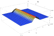
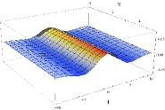
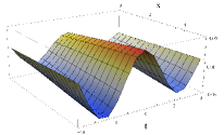
Figure 3: Wave profiles of exact solution (80) without white noise as $\alpha=0.25,0.5,1$.

Note that it satisfies $V_{1}(x,t)\rightarrow 0$ as $t\rightarrow\pm\infty$ for all $x$ as $\alpha=0.25,0.5$ and $V_{1}(x,t)\rightarrow 0$ as $t\rightarrow\infty$ for all $x$ as $\alpha=1$.

With $k=0.05$, $\mu(t)=-3$, $f_{1}(t)=-0.2$, $f_{2}(t)=10$, $f_{4}(t)=0.01\cos(0.5t)$, $c_{1}=c_{2}=c_{4}=1$ as $\alpha=0.25$, $0.5$, $1$, $W(t)=\sin(0.5t)$, we present the dynamics of the white noise functional exact solution (80) in Fig. 4.

   

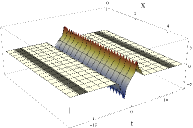
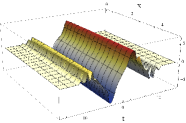
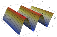
Figure 4: Wave profiles of exact solution (80) with white noise as $\alpha=0.25,0.5,1$.

Note that $V_{1}(x,t)\rightarrow 0$ as $t\rightarrow\pm\infty$ for all $x$ and the dynamics represent irregular movements in some interval of $t$ by employing white noise. For $\alpha=1$, it is like a periodic solution that satisfies $V_{1}(x,t)\rightarrow 0$ as $t\rightarrow\infty$ for all $x$. In Fig. 5, we provided the dynamics of exact solution (84) with $W(t)=0$, under $k=0.05$, $\mu(t)=-1.5$, $f_{1}(t)=-0.2$, $f_{2}(t)=10$, $f_{4}(t)=0.01\cos(0.5t)$, $c_{1}=c_{2}=c_{4}=1$. For $\alpha=0.25$, $0.5$, $1$, it gives $V_{4}(x,t)\rightarrow 0.018$ as $t\rightarrow\infty$ for all $x$.

   

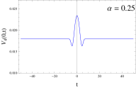
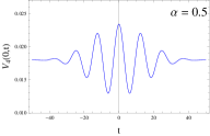
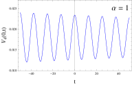
Figure 5: Wave motions of exact solution (84) without white noise as $\alpha=0.25,0.5,1$.

   

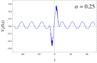
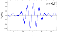
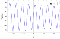
Figure 6: Wave motions of exact solution (84) with white noise as $\alpha=0.25,0.5,1$.

Under a white noise $W(t)=\sin(0.5t)$ and $k=0.05$, $\mu(t)=-1.5$, $f_{1}(t)=-0.2$, $f_{2}(t)=10$, $f_{4}(t)=0.01\cos(0.5t)$, $c_{1}=c_{2}=c_{4}=1$, for $\alpha=0.25,0.5,1$, Fig. 6 gives wave motions of the white noise functional solution of (84). It can be seen that the behaviors of exact solution $V_{4}(x,t)$ are roughly dynamic in $(-t_{0},t_{0})$ and it gives periodic wave motions in $(\infty,-t_{0})$ and $(t_{0},\infty)$ for $\alpha=0.25$ and $\alpha=0.5$. Furthermore, for $\alpha=1$, the values of $V_{4}(0,t)$ lies between $-0.08$ and $0.12$ as $t$ approaches $\infty$. From the simulations, it is concluded that we obtain different dynamics of the white noise functional solutions of Eq. (4) by the role of white noise as fractional orders.

4 Conclusion

In this paper, we obtained Wick-type exact solutions of the stochastic nonlinear Schrödinger and the Wick-type stochastic fractional RLW-Burgers equations by employing an improved computational method with integral and fractional order. Specifically, the Hermite transform is implemented, which changes Wick products into ordinary products and consequently converts Wick-type stochastic equations to deterministic nonlinear ordinary differential ones. Then we have applied the improved computational technique for determining exact traveling wave solutions for associated deterministic equations. Finally, the inverse Hermite transform is applied to obtained solutions for obtaining Wick-type exact solutions in the Wick type stochastic case.

References

- [1] X.-F. Pang, The properties of the solutions of nonlinear Schrödinger equation with center potential, Int. J. Nonlinear Sci. Numer. Simul. 15 (2014), no. 3-4, 215–219.
- [2] B. Kafash, R. Lalehzari, A. Delavarkhalafi and E. Mahmoudi, Application of stochastic differential system in chemical reactions via simulation, MATCH Commun. Math. Comput. Chem. 71 (2014), 265–277.
- [3] C. H. Lee and P. Kim, An analytical approach to solutions of master equations for stochastic nonlinear reactions, J. Math. Chem. 50 (2012), no. 6, 1550–1569.
- [4] H. Holden, B. Øksendal, J. Uboe and T. Zhang, Stochastic partial differential equations, Probability and its Applications, Birkhäuser Boston, Inc., Boston, MA, 1996.
- [5] H. Holden, B. Øksendal, J. Uboe and T. Zhang, Stochastic partial differential equations, second edition, Universitext, Springer, New York, 2010.
- [6] S. B. Zhang, Y. Wu and J. G. Wang, Time-dependent quantum wave packet dynamics to study charge transfer in heavy particle collisions, J. Chem. Phys. 145 (2016), no. 22, 224306.
- [7] C. Burgos, J. C. Cortés, A. Debbouche, L. Villafuerte and R. J. Villanueva, Random fractional generalized Airy differential equations: a probabilistic analysis using mean square calculus, Appl. Math. Comput. 352 (2019), 15–29.
- [8] H. Kim and R. Sakthivel, New travelling wave solutions for nonlinear stochastic evolution equations, Pramana J. Phys. 80 (2013), no. 6, 917–931.
- [9] J. H. Choi, H. Kim and R. Sakthivel, Exact solution of the Wick-type stochastic fractional coupled KdV equations, J. Math. Chem. 52 (2014), no. 10, 2482–2493.
- [10] S. Saha Ray and S. Singh, New exact solutions for the Wick-type stochastic modified Boussinesq equation for describing wave propagation in nonlinear dispersive systems, Chinese J. Phys. 55 (2017), 1653–1662.
- [11] S. Saha Ray and S. Singh, New exact solutions for the Wick-type stochastic Zakharov-Kuznetsov equation for modelling waves on shallow water surfaces, Random Oper. Stoch. Equ. 25 (2017), no. 2, 107–116.
- [12] H. A. Ghany, S. K. Elagan and A. Hyder, Exact travelling wave solutions for stochastic fractional Hirota-Satsuma coupled KdV equations, Chinese J. Phys. 53 (2015), no. 4, Art. ID 080705.
- [13] Y. Li, Y. Zhao and Z. Yao, Stochastic exact solutions of the Wick-type stochastic NLS equation, Appl. Math. Comput. 249 (2014), 209–221.
- [14] S. Saha Ray and S. Singh, New exact solutions for the Wick-type stochastic Kudryashov-Sinelshchikov equation, Commun. Theor. Phys. 67 (2017), 197–206.
- [15] S. Singh and S. Saha Ray, Exact solutions for the Wick-type stochastic Kersten-Krasilshchik coupled KdV-mKdV equations, S. Eur. Phys. J. Plus 132 (2017), 480.
- [16] N. M. Yazid, T. Kim, Y. Y. Choy and A. M. Sudin, Solving Nonlinear Schrodinger Equation with Variable Coefficient Using Homotopy Perturbation Method. In: Proceedings of the International Conference on Computing, Mathematics and Statistics (iCMS 2015), Springer, Singapore, 2017, 253–262.
- [17] F. Güngör, M. Hasanov and C. Özemir, A variable coefficient nonlinear Schrödinger equation with a four-dimensional symmetry group and blow-up, Appl. Anal. 92 (2013), no. 6, 1322–1331.
- [18] M. A. El-Tawil and A. S. Al-Jihany, On the solution of stochastic oscillatory quadratic nonlinear equations using different techniques, a comparison study, Topol. Methods Nonlinear Anal. 31 (2008), no. 2, 315–330.
- [19] C. Q. Dai and J. F. Zhang, Stochastic exact solutions and two-soliton solution of the Wick-type stochastic KdV equation, Europhys. Lett. 86 (2009), 40006–40008.
- [20] X.-J. Pan, C.-Q. Dai and L.-F. Mo, Analytical solutions for the stochastic Gardner equation, Comput. Math. Appl. 61 (2011), no. 8, 2138–2141.
- [21] Y. Li, Y. Zhao and Z. Yao, Stochastic exact solutions of the Wick-type stochastic NLS equation, Appl. Math. Comput. 249 (2014), 209–221.
- [22] M. A. Matlob and Y. Jamali, The concepts and applications of fractional order differential calculus in modelling of viscoelastic systems: A primer, Crit. Rev. Biomed. Eng. 47 (2019), no. 4, 249–276.
- [23] A. A. Tateishi, H. V. Ribeiro and E. K. Lenzi, The role of fractional time-derivative operatos on anomalous diffusion, Front. Phys. 5 (2017), Art. ID 52, 9 pp.
- [24] R. Garrappa, E. Kaslik and M. Popolizio, Evaluation of fractional integrals and derivatives of elementary functions: Overview and tutorial, Mathematics 7 (2019), no. 5, Art. ID 407, 21 pp.
- [25] R. Herrmann, Fractional calculus, World Scientific Publishing Co. Pte. Ltd., Hackensack, NJ, 2018.
- [26] P. Ostalczyk, Discrete fractional calculus, Series in Computer Vision, 4, World Scientific Publishing Co. Pte. Ltd., Hackensack, NJ, 2016.
- [27] Y. Povstenko, Linear fractional diffusion-wave equation for scientists and engineers, Springer, Cham, 2015.
- [28] S. K. Mitter, Filtering and stochastic control: a historical perspective, IEEE Control Systems Magazine 16 (1996), no. 3, 67–76.
- [29] M. R. Sidi Ammi, I. Jamiai and D. F. M. Torres, A finite element approximation for a class of Caputo time-fractional diffusion equations, Comput. Math. Appl. 78 (2019), no. 5, 1334–1344. arXiv:1905.10657
- [30] M. R. Sidi Ammi and D. F. M. Torres, Optimal control of a nonlocal thermistor problem with ABC fractional time derivatives, Comput. Math. Appl. 78 (2019), no. 5, 1507–1516. arXiv:1903.07961
- [31] N. H. Tuan, A. Debbouche and T. B. Ngoc, Existence and regularity of final value problems for time fractional wave equations, Comput. Math. Appl. 78 (2019), no. 5, 1396–1414.
- [32] Y. Zhou, L. Shangerganesh, J. Manimaran and A. Debbouche, A class of time-fractional reaction-diffusion equation with nonlocal boundary condition, Math. Methods Appl. Sci. 41 (2018), no. 8, 2987–2999.
- [33] J. Manimaran, L. Shangerganesh, A. Debbouche and V. Antonov, Numerical solutions for time-fractional cancer invasion system with nonlocal diffusion, Frontiers in Physics 7 (2019), 93.
- [34] A. Atangana and I. Koca, Chaos in a simple nonlinear system with Atangana-Baleanu derivatives with fractional order, Chaos Solitons Fractals 89 (2016), 447–454.
- [35] R. Hilfer, Applications of fractional calculus in physics, World Scientific Publishing Co., Inc., River Edge, NJ, 2000.
- [36] S. Zhang and H.-Q. Zhang, Fractional sub-equation method and its applications to nonlinear fractional PDEs, Phys. Lett. A 375 (2011), no. 7, 1069–1073.
- [37] J. L. Bona, W. G. Pritchard and L. R. Scott, An evaluation of a model equation for water waves, Philos. Trans. Roy. Soc. London Ser. A 302 (1981), no. 1471, 457–510.
- [38] H. Holden, B. Øsandal, J. Uboe and T. Zhang, Stochastic partial differential equations, Probability and its Applications, Birkhäuser Boston, Inc., Boston, MA, 1996.
- [39] A. A. Kilbas, H. M. Srivastava and J. J. Trujillo, Theory and applications of fractional differential equations, North-Holland Mathematics Studies, 204, Elsevier Science B.V., Amsterdam, 2006.
- [40] F. E. Benth and J. Gjerde, A remark on the equivalence between Poisson and Gaussian stochastic partial differential equations, Potential Anal. 8 (1998), no. 2, 179–193.
- [41] C. Q. Dai and J. F. Zhang, Stochastic exact solutions and two-soliton solution of the Wick-type stochastic KdV equation, Europhys. Lett. 86 (2009), 40006–40008.
- [42] Y. Chen, Q. Wang and B. Li, The stochastic soliton-like solutions of stochastic KdV equations, Chaos Solitons Fractals 23 (2005), no. 4, 1465–1473.
- [43] Y. Xie, Positonic solutions for Wick-type stochastic KdV equations, Chaos Solitons Fractals 20 (2004), no. 2, 337–342.
- [44] M. Z. Gorgulu, I. Dag and D. Irk, Simulations of solitary waves of RLW equation by exponential B-spline Galerkin method, Chin. Phys. B 26 (2017), no. 8, 080202.
- [45] S. Abbasbandy and A. Shirzadi, The first integral method for modified Benjamin-Bona-Mahony equation, Commun. Nonlinear Sci. Numer. Simul. 15 (2010), no. 7, 1759–1764.