Vibration Suppression for Coupled Wave PDEs
in Deep-sea Construction

Ji Wang, , and Miroslav Krstic J. Wang and M. Krstic are with Department of Mechanical and Aerospace Engineering, University of California, San Diego, La Jolla, CA 92093-0411, USA(e-mail: jiwang9024@gmail.com;krstic@ucsd.edu).
Abstract

A deep-sea construction vessel is used to install underwater parts of an off-shore oil drilling platform at the designated locations on the seafloor. By using extended Hamilton’s principle, a nonlinear PDE system governing the lateral-longitudinal coupled vibration dynamics of the deep-sea construction vessel consisting of a time-varying-length cable with an attached item is derived, and it is linearized at the steady state generating a linear PDE model, which is extended to a more general system including two coupled wave PDEs connected with two interacting ODEs at the uncontrolled boundaries. Through a preliminary transformation, an equivalent reformulated plant is generated as a 4×4444\times 4 coupled heterodirectional hyperbolic PDE-ODE system characterized by spatially-varying coefficients on a time-varying domain. To stabilize such a system, an observer-based output-feedback control design is proposed, where the measurements are only placed at the actuated boundary of the PDE, namely, at the platform at the sea surface. The exponential stability of the closed-loop system, boundedness and exponential convergence of the control inputs, are proved via Lyapunov analysis. The obtained theoretical result is tested on a nonlinear model with ocean disturbances, even though the design is developed in the absence of such real-world effects.

Index Terms:
wave PDE, distributed parameter system, boundary control, backstepping, vibration control.

I Introduction

Deep-sea construction vessels

In deep-sea oil exploration, a deep-sea construction vessel (DCV) is an important device used to install equipment such as a subsea manifold, a subsea pump station, flowlines and so on, at the designated locations around the drill center on the seafloor [25, 26]. A dominant component in the DCV is a long cable with time-varying length, of which the top is attached to a ship-mounted crane and the bottom is attached to the equipment (referred to as payloads hereafter). Excessive vibration of the cable due to its compliant and lightweight properties is a major problem affecting the payload positioning precision of the DCV. Besides, the excessive vibration also may cause premature fatigue fracture of the cable especially at the connection point [18], which would raise the cost of part replacement or maintenance of the DCV. Therefore, vibration suppression for the cable in the DCV is well motivated for improving performance of the DCV.

Vibration control of string/cable

Vibration control of a string/cable has received much attention in the past several decades. An active vibration control strategy was designed for a vibrational string in [36], where the actuator and sensor are required to be placed at the interior point of the cable. [18, 19] suppressed the undesired vibrations of a moving vibrational string by applying control inputs at both boundaries. In [37], robust adaptive vibration control was proposed for a disturbed vibrating string of which one boundary is fixed and the opposite one is connected with a payload regulated by the control input. However, the required actuator layouts of the aforementioned control systems are unsuitable for the DCV where the actuator is only available at the ship-mounted crane, i.e., the top end of the cable.

Boundary control of wave PDE-ODE systems

The mathematical model of a vibrational string/cable is a wave partial differential equation (PDE), and the attached payload is modeled as an ordinary differential equation (ODE) at the PDE uncontrolled boundary. Boundary control of a wave PDE-ODE systems where the control input and the unstable ODE are anti-collocated is a more challenging task than the classical collocated “boundary damper” feedback control. Stabilization of such a wave PDE-ODE system on a fixed domain was presented in [20, 27]. For a wave PDE-nonlinear ODE system, the boundary control problem is also studied in [8, 10]. References [32, 33] presented boundary control of a wave PDE-ODE coupled system on a time-varying domain, which physically describes the axial vibration of a mining cable elevator. Adaptive boundary control of a wave PDE-ODE coupled system with unknown parameters was also considered in [31]. The aforementioned works only concern a single wave PDE describing vibrations in one-direction. Challenges appear in the suppression of two-dimensional string vibrations, because there are in-domain couplings between two wave PDEs.

Boundary control of coupled heterodirectional transport PDEs

A feasible approach to solving the boundary control problem of in-domain coupled wave PDEs is by introducing Riemann transformations to convert the plant to coupled transport PDEs, for which the boundary control problem has been a research focus for the past ten years, with many authors contributing to this topic. Basic boundary stabilization of a 2×2222\times 2 coupled linear transport PDEs, i.e., two heterodirectional coupled transport PDEs, by backstepping was proposed in [28, 9]. It was further extended to boundary control of a n+1𝑛1n+1 system in [22]. For a more general coupled linear transport PDE system where the number of PDEs in either direction is arbitrary, the boundary stabilization problem was first addressed in [17] by backstepping, which leads to a systematic framework for the backstepping-based control of this type of system. Moreover, adaptive control with unknown system parameters or disturbance rejection for external periodic disturbances in coupled heterodirectional transport PDEs, have appeared in [3, 4] and [11, 12, 2, 1] respectively. Considering the attached massive payload at the bottom of the cable, boundary control of coupled linear transport PDEs connected with an ODE at the uncontrolled boundary can also be found in [23, 35, 13]. The aforementioned works on coupled transport PDEs focus on the constant spatial domain rather than a time-varying domain introduced by the time-varying length of the cable.

Contribution
  • To the best of our knowledge, our result is the first for boundary control of a two-dimensional coupled vibrating cable of time-varying length, where only one control input is applied at one boundary without requirements of energy dissipation or another controller on another boundary.

  • A similar physical problem was considered in [5] which presented state-feedback control design while neglecting the couplings between two directions of vibration and assuming the cable length as constant. An observer-based output-feedback is proposed here, considering the coupled vibrations of a time-varying-length cable.

  • [23] first proposed a full-state feedback law needing measurements of the distributed states for a general coupled linear heterodirectional hyperbolic PDE-ODE system on a fixed domain. We develop a design for such systems on a time-varying domain, and using only measurements at the actuated boundary.

  • As compared to our previous results about longitudinal vibration suppression control of cables in PDE-modeled mining cable elevators [32, 33, 34], this paper achieves suppression of longitudinal-lateral coupled vibrations in cables, where the in-domain couplings between wave PDEs, i.e., the couplings between two direction vibrations, make the control design more challenging.

For complete clarity, the comparisons with our previous results and other related results from the theoretical and application aspects are summarized in Tab. I-II respectively.

TABLE I: Comparisons with application results on boundary vibration control of cables.
Multi-dimensional Time-varying Number of
coupled vibrations cable controlled/fixed/
in cables lengths damped boundaries
[18, 21] ×\times square-root\surd 2
[19] square-root\surd square-root\surd 2
[5] square-root\surd ×\times 1
[32]-[34] ×\times square-root\surd 1
This paper square-root\surd square-root\surd 1
TABLE II: Comparisons with recent theoretical results on boundary control of linear coupled transport PDEs-ODE systems.
Types of Spatially-varying Time-varying Measurements
hyperbolic PDEs coefficients domain
[23] n𝑛n coupled transport PDEs square-root\surd ×\times Full distributed states
[13] n𝑛n coupled transport PDEs square-root\surd ×\times States at the uncontrolled boundary
[29] 2×2222\times 2 coupled transport PDEs ×\times ×\times Output states of ODE at the uncontrolled boundary
[34] 2×2222\times 2 coupled transport PDEs ×\times square-root\surd States at two boundaries
This paper 4×4444\times 4 coupled transport PDEs square-root\surd square-root\surd States at the actuated boundary
Organization

This paper is organized as follows. In Section II, a nonlinear distributed parameter model governing the longitudinal-lateral vibration dynamics of the DCV is derived by Hamilton’s principle, which is then linearized around the steady state and extend to a general plant, based on which the control design would be conducted in the following sections. In Section III, the state-feedback control design is presented and the exponential stability result of the state-feedback closed-loop system is proved. In Section IV, we design a state observer and prove the exponential convergence to zero of observer errors. In Section V, we propose an observer-based output-feedback controller and establish the main result in the output-feedback closed-loop system. In Section VI, the obtained theoretical result is tested on a nonlinear model with ocean disturbances, even though the design is developed in the absence of such real-world effects. In Section VII, the conclusion and future work are provided.

Notation

Throughout this paper, the partial derivatives and total derivatives are denoted as: fx(x,t)=fx(x,t)subscript𝑓𝑥𝑥𝑡𝑓𝑥𝑥𝑡{f_{x}}(x,t)=\frac{{\partial f}}{{\partial x}}(x,t), ft(x,t)=ft(x,t)subscript𝑓𝑡𝑥𝑡𝑓𝑡𝑥𝑡{f_{t}}(x,t)=\frac{{\partial f}}{{\partial t}}(x,t), f(x)=df(x)dxsuperscript𝑓𝑥𝑑𝑓𝑥𝑑𝑥f^{\prime}(x)=\frac{{df(x)}}{{dx}}, f˙(t)=df(t)dt˙𝑓𝑡𝑑𝑓𝑡𝑑𝑡\dot{f}(t)=\frac{{df(t)}}{{dt}}.

II Problem Formulation

II-A Modeling

Refer to caption
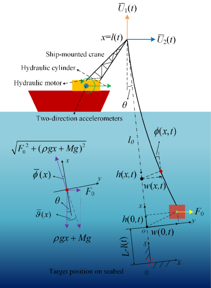
Figure 1: Diagram of a deep-sea construction vessel.

DCVs are often used for installation of underwater parts for an offshore drilling platform, such as a subsea manifold, a subsea pump station, a subsea distribution unit along with associated foundations, flowlines and umbilicals [25]-[26]. A DCV is depicted in Fig. 1, where a crane mounted on a ship regulates a cable to install an equipment (attached payload) at the target position on the seabed. The attached payload is subject to a constant drag force caused by a constant water stream velocity. We only consider the water-stream caused drag force at the payload because the diameter of the cable is much smaller than that of the payload. For suppression of cable oscillation/vibration, two-directional control forces implemented by two actuators (hydraulic cylinder and hydraulic motor) and measurements by accelerometers are applied/placed at the ship-mounted crane. Note that cable motion is provided by an additional winch winded by cable on the ship, which can be considered as a pre-defined time-varying function l(t)𝑙𝑡l(t) of cable length in the cable vibration dynamics regulated by the cranes.

Hamilton’s principle [24] is applied to formulate the mathematical model of the two-dimensional vibrations of the DCV in Fig. 1, where we neglect the dynamics of the ship because it can be kept at the desired position by the ship dynamic positioning system. The physical parameters of the DCV are shown in Table III and the given values are used in the simulation. To describe the vibrations of the cable, the classical moving frame approach is used [6]. In Fig. 1, the xoy𝑥𝑜𝑦xoy frame is a moving coordinate associated with cable motion, i.e., the time-varying cable length l(t)𝑙𝑡l(t), moving along line lθsubscript𝑙𝜃l_{\theta}, where x𝑥x ranges from x=0𝑥0x=0 at the cable bottom to x=l(t)𝑥𝑙𝑡x=l(t) at the top end. The other coordinate frame x¯o¯y¯¯𝑥¯𝑜¯𝑦\underline{x}\underline{o}\underline{y} is earth fixed. Buoyancy on the cable can easily be included by adjusting the cable linear density mcsubscript𝑚𝑐m_{c} as ρ=mcρwAa𝜌subscript𝑚𝑐subscript𝜌𝑤subscript𝐴𝑎\rho=m_{c}-\rho_{w}A_{a}, and changing the payload mass MLsubscript𝑀𝐿M_{L} as M=MLρwVp𝑀subscript𝑀𝐿subscript𝜌𝑤subscript𝑉𝑝M=M_{L}-\rho_{w}V_{p}, when calculate the gravity of the payload.

Denote the longitudinal and (in-plane) lateral dynamic deflections in the distributed position x𝑥x in the cable as h(x,t)𝑥𝑡h(x,t) and w(x,t)𝑤𝑥𝑡w(x,t), respectively. The deformed position vector, i.e., vibration displacement vector, in the earth fixed coordinate frame x¯o¯y¯¯𝑥¯𝑜¯𝑦\underline{x}\underline{o}\underline{y} is

D(x,t)=[Ll(t)+x+h(x,t),w(x,t)]T.𝐷𝑥𝑡superscript𝐿𝑙𝑡𝑥𝑥𝑡𝑤𝑥𝑡𝑇\displaystyle D(x,t)=[L-l(t)+x+h(x,t),w(x,t)]^{T}. (1)

Thus, the velocity vector is

Dt(x,t)=[ht(x,t)l˙(t),wt(x,t)]T.subscript𝐷𝑡𝑥𝑡superscriptsubscript𝑡𝑥𝑡˙𝑙𝑡subscript𝑤𝑡𝑥𝑡𝑇\displaystyle D_{t}(x,t)=[h_{t}(x,t)-\dot{l}(t),w_{t}(x,t)]^{T}. (2)

According to the large displacement approach [7], the strain at the distributed positions x𝑥x in the cable is given by

ε(x,t)=hx(x,t)+12wx(x,t)2.𝜀𝑥𝑡subscript𝑥𝑥𝑡12subscript𝑤𝑥superscript𝑥𝑡2\displaystyle\varepsilon(x,t)={h_{x}}(x,t)+\frac{1}{2}{w_{x}}{{(x,t)}^{2}}. (3)

Therefore, the kinetic energy Eksubscript𝐸𝑘E_{k} and the potential energy Epsubscript𝐸𝑝E_{p} of the system are represented as

Eksubscript𝐸𝑘\displaystyle E_{k} =ρ20l(t)Dt(x,t)2𝑑x+ML2Dt(0,t)2,absent𝜌2superscriptsubscript0𝑙𝑡subscript𝐷𝑡superscript𝑥𝑡2differential-d𝑥subscript𝑀𝐿2subscript𝐷𝑡superscript0𝑡2\displaystyle=\frac{\rho}{2}\int_{0}^{l(t)}{{D_{t}}{{(x,t)}^{2}}}dx+\frac{M_{L}}{2}{D_{t}}{(0,t)^{2}}, (4)
Epsubscript𝐸𝑝\displaystyle E_{p} =120l(t)EAaε(x,t)2𝑑x+0l(t)T(x,t)ε(x,t)𝑑x,absent12superscriptsubscript0𝑙𝑡𝐸subscript𝐴𝑎𝜀superscript𝑥𝑡2differential-d𝑥superscriptsubscript0𝑙𝑡𝑇𝑥𝑡𝜀𝑥𝑡differential-d𝑥\displaystyle=\frac{1}{2}\int_{0}^{l(t)}{EA_{a}\varepsilon{{(x,t)}^{2}}}dx+\int_{0}^{l(t)}{T(x,t)\varepsilon(x,t)}dx, (5)

where T(x)𝑇𝑥T(x) is static tension given by

T(x)=ρgx+Mg.𝑇𝑥𝜌𝑔𝑥𝑀𝑔\displaystyle T(x)=\rho gx+Mg. (6)

Because the long steel cable and the equipment at the bottom of the cable are very heavy and the resulting gravity is much larger than the water-stream caused drag force F0=ρw2CdVs2subscript𝐹0subscript𝜌𝑤2subscript𝐶𝑑superscriptsubscript𝑉𝑠2F_{0}=\frac{\rho_{w}}{2}C_{d}V_{s}^{2} [5], the angle θ=arctanF0ρgL+Mg𝜃subscript𝐹0𝜌𝑔𝐿𝑀𝑔\theta=\arctan\frac{F_{0}}{\sqrt{\rho gL+Mg}} in Fig. 1 is thus small. Therefore, it is reasonable to assume that the static tension T(x)𝑇𝑥T(x) only results from the mass of the payload and cable.

TABLE III: Physical parameters of the DCV.
Parameters (units) values
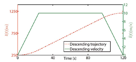
Final cable length L𝐿{L} (m) 1210
Initial cable length l(0)𝑙0l(0) (m) 250
Maximum descending velocity M¯¯𝑀\bar{M} (m/s) 10
Operation time tfsubscript𝑡𝑓t_{f} (s) 120
Cable cross-sectional area Aasubscript𝐴𝑎{A_{a}} (m2) 0.47×{\times}103superscript103{10^{-3}}
Cable effective Young s Modulus E𝐸E (N/m2) 7.03×\times1010superscript1010{10^{10}}
Cable linear density mcsubscript𝑚𝑐m_{c} (kg/m) 8. 95
Payload mass MLsubscript𝑀𝐿{M_{L}} (kg) 8000
Payload volume Vpsubscript𝑉𝑝V_{p} (m3superscript𝑚3m^{3}) 5
Gravitational acceleration g (m/s2) 9.8
Drag coefficient Cdsubscript𝐶𝑑C_{d} 1
Stream velocity Vssubscript𝑉𝑠V_{s} (m/s) 2
Seawater density ρwsubscript𝜌𝑤\rho_{w} (kgm3𝑘𝑔superscript𝑚3kgm^{-3}) 1024
Longitudinal damping coefficient in cable cusubscript𝑐𝑢c_{u} 0.5
Lateral damping coefficient in cable cvsubscript𝑐𝑣c_{v} 0.3
Longitudinal damping coefficient at attached payload chsubscript𝑐c_{h} 0.5
Lateral damping coefficient at attached payload cwsubscript𝑐𝑤c_{w} 0.3

The virtual work is

δW=𝛿𝑊absent\displaystyle\delta W= U¯1δh(l(t),t)+U¯2δw(l(t),t)+ch(ht(0,t)l˙(t))δh(0,t)subscript¯𝑈1𝛿𝑙𝑡𝑡subscript¯𝑈2𝛿𝑤𝑙𝑡𝑡subscript𝑐subscript𝑡0𝑡˙𝑙𝑡𝛿0𝑡\displaystyle{\bar{U}_{1}}\delta h(l(t),t)+{\bar{U}_{2}}\delta w(l(t),t)+c_{h}({h_{t}}(0,t)-\dot{l}(t))\delta h(0,t)
+cwwt(0,t)δw(0,t)+0l(t)cvwt(x,t)δw(x,t)𝑑xsubscript𝑐𝑤subscript𝑤𝑡0𝑡𝛿𝑤0𝑡superscriptsubscript0𝑙𝑡subscript𝑐𝑣subscript𝑤𝑡𝑥𝑡𝛿𝑤𝑥𝑡differential-d𝑥\displaystyle+{c_{w}}{w_{t}}(0,t)\delta w(0,t)+\int_{0}^{l(t)}{{c_{v}}{w_{t}}(x,t)\delta}w(x,t)dx
+0l(t)cu(ht(x,t)l˙(t))δh(x,t)𝑑x+F0δw(0,t)superscriptsubscript0𝑙𝑡subscript𝑐𝑢subscript𝑡𝑥𝑡˙𝑙𝑡𝛿𝑥𝑡differential-d𝑥subscript𝐹0𝛿𝑤0𝑡\displaystyle+\int_{0}^{l(t)}{c_{u}}({h_{t}}(x,t)-\dot{l}(t))\delta h(x,t)dx+F_{0}\delta w(0,t)
Mgδh(0,t)0l(t)ρgδh(x,t)𝑑x.𝑀𝑔𝛿0𝑡superscriptsubscript0𝑙𝑡𝜌𝑔𝛿𝑥𝑡differential-d𝑥\displaystyle-Mg\delta h(0,t)-\int_{0}^{l(t)}{\rho g\delta h(x,t)}dx. (7)

Note that an approximation is adopted in the virtual work (7), that the virtual work done by the gravity and U1subscript𝑈1U_{1} are parallel to x𝑥x-direction, and the virtual work done by F0subscript𝐹0F_{0} and U2subscript𝑈2U_{2} are parallel to y𝑦y-direction, due to the small θ𝜃\theta.

Apply variations of (4)-(5) into extended Hamilton’s principle

t1t2(δEkδEp+δW)𝑑t=0,superscriptsubscriptsubscript𝑡1subscript𝑡2𝛿subscript𝐸𝑘𝛿subscript𝐸𝑝𝛿𝑊differential-d𝑡0\displaystyle\int_{t_{1}}^{t_{2}}(\delta E_{k}-\delta E_{p}+\delta W)dt=0, (8)

where a difference from the standard procedure due to the time-varying integration domain should be noted as (9)-(10),

ρ0l(t)Dt(x,t)δDt(x,t)𝑑x𝜌superscriptsubscript0𝑙𝑡subscript𝐷𝑡𝑥𝑡𝛿subscript𝐷𝑡𝑥𝑡differential-d𝑥\displaystyle\rho\int_{0}^{l(t)}{{D_{t}}(x,t)\delta{D_{t}}(x,t)}dx
=ρ0l(t)Dt(x,t)δD(x,t)𝑑xdtl˙(t)ρDt(l(t),t)δD(l(t),t)absent𝜌superscriptsubscript0𝑙𝑡subscript𝐷𝑡𝑥𝑡𝛿𝐷𝑥𝑡differential-d𝑥𝑑𝑡˙𝑙𝑡𝜌subscript𝐷𝑡𝑙𝑡𝑡𝛿𝐷𝑙𝑡𝑡\displaystyle=\frac{{\rho\int_{0}^{l(t)}{{D_{t}}(x,t)\delta D(x,t)}dx}}{{dt}}-\dot{l}(t)\rho{D_{t}}(l(t),t)\delta D(l(t),t)
ρ0l(t)Dtt(x,t)δD(x,t)𝑑x,𝜌superscriptsubscript0𝑙𝑡subscript𝐷𝑡𝑡𝑥𝑡𝛿𝐷𝑥𝑡differential-d𝑥\displaystyle-\rho\int_{0}^{l(t)}{{D_{tt}}(x,t)\delta D(x,t)}dx, (9)

integrating (9) from t1subscript𝑡1t_{1} to t2subscript𝑡2t_{2} then yields

t1t2ρ0l(t)Dt(x,t)δDt(x,t)𝑑x𝑑tsuperscriptsubscriptsubscript𝑡1subscript𝑡2𝜌superscriptsubscript0𝑙𝑡subscript𝐷𝑡𝑥𝑡𝛿subscript𝐷𝑡𝑥𝑡differential-d𝑥differential-d𝑡\displaystyle\int_{{t_{1}}}^{{t_{2}}}\rho\int_{0}^{l(t)}{{D_{t}}(x,t)\delta{D_{t}}(x,t)}dxdt
=t1t2l˙(t)ρDt(l(t),t)δD(l(t),t)𝑑tabsentsuperscriptsubscriptsubscript𝑡1subscript𝑡2˙𝑙𝑡𝜌subscript𝐷𝑡𝑙𝑡𝑡𝛿𝐷𝑙𝑡𝑡differential-d𝑡\displaystyle=-\int_{{t_{1}}}^{{t_{2}}}\dot{l}(t)\rho{D_{t}}(l(t),t)\delta D(l(t),t)dt
t1t2ρ0l(t)Dtt(x,t)δD(x,t)𝑑x𝑑t.superscriptsubscriptsubscript𝑡1subscript𝑡2𝜌superscriptsubscript0𝑙𝑡subscript𝐷𝑡𝑡𝑥𝑡𝛿𝐷𝑥𝑡differential-d𝑥differential-d𝑡\displaystyle-\int_{{t_{1}}}^{{t_{2}}}\rho\int_{0}^{l(t)}{{D_{tt}}(x,t)\delta D(x,t)}dxdt. (10)

Note that l(t)𝑙𝑡l(t) is treated as a pre-defined function and thus it is not necessary to consider its variation in δD(x,t),δDt(x,t)𝛿𝐷𝑥𝑡𝛿subscript𝐷𝑡𝑥𝑡\delta{D}(x,t),\delta{D_{t}}(x,t), i.e., δl(t)=δl˙(t)=0𝛿𝑙𝑡𝛿˙𝑙𝑡0\delta l(t)=\delta\dot{l}(t)=0.

Through a lengthy calculation for (8), the following governing equations are then obtained as

mc(htt(x,t)l¨(t))+EAahxx(x,t)subscript𝑚𝑐subscript𝑡𝑡𝑥𝑡¨𝑙𝑡𝐸subscript𝐴𝑎subscript𝑥𝑥𝑥𝑡\displaystyle-m_{c}({h_{tt}}(x,t)-\ddot{l}(t))+EA_{a}{h_{xx}}(x,t)
+cu(ht(x,t)l˙(t))+EAawx(x,t)wxx(x,t)=0,subscript𝑐𝑢subscript𝑡𝑥𝑡˙𝑙𝑡𝐸subscript𝐴𝑎subscript𝑤𝑥𝑥𝑡subscript𝑤𝑥𝑥𝑥𝑡0\displaystyle+{c_{u}}({h_{t}}(x,t)-\dot{l}(t))+EA_{a}{w_{x}}(x,t){w_{xx}}(x,t)=0, (11)
mcwtt(x,t)+32EAawx(x,t)2wxx(x,t)+T(x)wxx(x,t)subscript𝑚𝑐subscript𝑤𝑡𝑡𝑥𝑡32𝐸subscript𝐴𝑎subscript𝑤𝑥superscript𝑥𝑡2subscript𝑤𝑥𝑥𝑥𝑡𝑇𝑥subscript𝑤𝑥𝑥𝑥𝑡\displaystyle-m_{c}{w_{tt}}(x,t)+\frac{3}{2}EA_{a}{w_{x}}{(x,t)^{2}}{w_{xx}}(x,t)+T(x){w_{xx}}(x,t)
+EAahx(x,t)wxx(x,t)+EAahxx(x,t)wx(x,t)𝐸subscript𝐴𝑎subscript𝑥𝑥𝑡subscript𝑤𝑥𝑥𝑥𝑡𝐸subscript𝐴𝑎subscript𝑥𝑥𝑥𝑡subscript𝑤𝑥𝑥𝑡\displaystyle+EA_{a}{h_{x}}(x,t){w_{xx}}(x,t)+EA_{a}{h_{xx}}(x,t){w_{x}}(x,t)
+cvwt(x,t)+T(x)wx(x,t)=0,subscript𝑐𝑣subscript𝑤𝑡𝑥𝑡superscript𝑇𝑥subscript𝑤𝑥𝑥𝑡0\displaystyle+{c_{v}}{w_{t}}(x,t)+T^{\prime}(x){w_{x}}(x,t)=0, (12)
ML(htt(0,t)l¨(t))+ch(ht(0,t)l˙(t))+EAahx(0,t)subscript𝑀𝐿subscript𝑡𝑡0𝑡¨𝑙𝑡subscript𝑐subscript𝑡0𝑡˙𝑙𝑡𝐸subscript𝐴𝑎subscript𝑥0𝑡\displaystyle M_{L}({h_{tt}}(0,t)-\ddot{l}(t))+c_{h}({h_{t}}(0,t)-\dot{l}(t))+EA_{a}{h_{x}}(0,t)
+12EAawx(0,t)2=0,12𝐸subscript𝐴𝑎subscript𝑤𝑥superscript0𝑡20\displaystyle+\frac{1}{2}EA_{a}{w_{x}}{(0,t)^{2}}=0, (13)
MLwtt(0,t)+cwwt(0,t)+12EAawx(0,t)3subscript𝑀𝐿subscript𝑤𝑡𝑡0𝑡subscript𝑐𝑤subscript𝑤𝑡0𝑡12𝐸subscript𝐴𝑎subscript𝑤𝑥superscript0𝑡3\displaystyle M_{L}{w_{tt}}(0,t)+{c_{w}}{w_{t}}(0,t)+\frac{1}{2}EA_{a}{w_{x}}{(0,t)^{3}}
+EAahx(0,t)wx(0,t)+T(0)wx(0,t)+F0=0,𝐸subscript𝐴𝑎subscript𝑥0𝑡subscript𝑤𝑥0𝑡𝑇0subscript𝑤𝑥0𝑡subscript𝐹00\displaystyle+EA_{a}{h_{x}}(0,t){w_{x}}(0,t)+T(0){w_{x}}(0,t)+F_{0}=0, (14)
(EAa(hx(l(t),t)+12wx(l(t),t)2)+T(l(t)))wx(l(t),t)𝐸subscript𝐴𝑎subscript𝑥𝑙𝑡𝑡12subscript𝑤𝑥superscript𝑙𝑡𝑡2𝑇𝑙𝑡subscript𝑤𝑥𝑙𝑡𝑡\displaystyle-\left(EA_{a}({h_{x}}(l(t),t)+\frac{1}{2}{w_{x}}{(l(t),t)^{2}})+T(l(t))\right){w_{x}}(l(t),t)
l˙(t)ρwt(l(t),t)+U¯2(t)=0,˙𝑙𝑡𝜌subscript𝑤𝑡𝑙𝑡𝑡subscript¯𝑈2𝑡0\displaystyle-\dot{l}(t)\rho{w_{t}}(l(t),t)+{\bar{U}_{2}}(t)=0, (15)
EAa(hx(l(t),t)+12wx(l(t),t)2)T(l(t))𝐸subscript𝐴𝑎subscript𝑥𝑙𝑡𝑡12subscript𝑤𝑥superscript𝑙𝑡𝑡2𝑇𝑙𝑡\displaystyle-EA_{a}\left({h_{x}}(l(t),t)+\frac{1}{2}{w_{x}}{(l(t),t)^{2}}\right)-T(l(t))
l˙(t)ρ(ht(l(t),t)l˙(t))+U¯1(t)=0.˙𝑙𝑡𝜌subscript𝑡𝑙𝑡𝑡˙𝑙𝑡subscript¯𝑈1𝑡0\displaystyle-\dot{l}(t)\rho({h_{t}}(l(t),t)-\dot{l}{(t)})+{\bar{U}_{1}}(t)=0. (16)

Note that crane dynamics are neglected and the control input is considered to act on the top end of the cable directly. Incorporating the crane dynamics into the actuation path of the cable would generate an ODE-coupled hyperbolic PDEs-ODE system. Control problem of such a sandwiched system was addressed in [29] which, however, only dealt with one-dimensional vibrations of DCV with a constant-length cable.

(11)-(16) is a strongly nonlinear system, so an approximated linear model that is suitable for control design should be built. The nonlinear PDE system (11)-(16) is linearized in the next subsection around a steady state as in the procedure in [5] .

II-B Linearization

The steady states of the distributed strain and pivot angle ε(x,t),ϕ(x,t)𝜀𝑥𝑡italic-ϕ𝑥𝑡\varepsilon(x,t),\phi(x,t) can be calculated analytically and expressed as

ε¯(x)¯𝜀𝑥\displaystyle\bar{\varepsilon}(x) =1EAa(ρgx+Mg)2+F02,absent1𝐸subscript𝐴𝑎superscript𝜌𝑔𝑥𝑀𝑔2superscriptsubscript𝐹02\displaystyle=\frac{1}{EA_{a}}\sqrt{(\rho gx+Mg)^{2}+F_{0}^{2}}, (17)
ϕ¯(x)¯italic-ϕ𝑥\displaystyle\bar{\phi}(x) =ϑ¯(x)θ=arctan(F0ρgx+Mg)θ.absent¯italic-ϑ𝑥𝜃subscript𝐹0𝜌𝑔𝑥𝑀𝑔𝜃\displaystyle=\bar{\vartheta}(x)-\theta=\arctan\left(\frac{F_{0}}{\rho gx+Mg}\right)-\theta. (18)

In nonlinear terms in (11)-(16), replacing hx(x,t)subscript𝑥𝑥𝑡h_{x}(x,t) which approximately describes the distributed strain in the cable by ε¯(x)¯𝜀𝑥\bar{\varepsilon}(x) , and replacing wx(x,t)subscript𝑤𝑥𝑥𝑡-w_{x}(x,t) which is approximately equal to the pivot angle ϕ(x,t)italic-ϕ𝑥𝑡\phi(x,t) in Fig. 1 by ϕ¯(x)¯italic-ϕ𝑥\bar{\phi}(x), a linear model around the steady state can be obtained as

mcutt(x,t)+EAauxx(x,t)EAawx(x,t)ϕ¯(x)subscript𝑚𝑐subscript𝑢𝑡𝑡𝑥𝑡𝐸subscript𝐴𝑎subscript𝑢𝑥𝑥𝑥𝑡𝐸subscript𝐴𝑎subscript𝑤𝑥𝑥𝑡superscript¯italic-ϕ𝑥\displaystyle-m_{c}{u_{tt}}(x,t)+EA_{a}{u_{xx}}(x,t)-EA_{a}{w_{x}}(x,t)\bar{\phi}^{\prime}(x)
+cuut(x,t)=0,subscript𝑐𝑢subscript𝑢𝑡𝑥𝑡0\displaystyle+{c_{u}}{u_{t}}(x,t)=0, (19)
mcwtt(x,t)+(32EAaϕ¯(x)2+T(x))wxx(x,t)subscript𝑚𝑐subscript𝑤𝑡𝑡𝑥𝑡32𝐸subscript𝐴𝑎¯italic-ϕsuperscript𝑥2𝑇𝑥subscript𝑤𝑥𝑥𝑥𝑡\displaystyle-m_{c}{w_{tt}}(x,t)+\left(\frac{3}{2}EA_{a}\bar{\phi}(x)^{2}+T(x)\right){w_{xx}}(x,t)
+(EAaε¯(x)+ρg)wx(x,t)𝐸subscript𝐴𝑎superscript¯𝜀𝑥𝜌𝑔subscript𝑤𝑥𝑥𝑡\displaystyle+(EA_{a}\bar{\varepsilon}^{\prime}(x)+\rho g){w_{x}}(x,t)
+cvwt(x,t)EAaϕ¯(x)ux(x,t)=0,subscript𝑐𝑣subscript𝑤𝑡𝑥𝑡𝐸subscript𝐴𝑎superscript¯italic-ϕ𝑥subscript𝑢𝑥𝑥𝑡0\displaystyle+{c_{v}}{w_{t}}(x,t)-EA_{a}\bar{\phi}^{\prime}(x){u_{x}}(x,t)=0, (20)
MLutt(0,t)+chut(0,t)+EAaux(0,t)subscript𝑀𝐿subscript𝑢𝑡𝑡0𝑡subscript𝑐subscript𝑢𝑡0𝑡𝐸subscript𝐴𝑎subscript𝑢𝑥0𝑡\displaystyle M_{L}{u_{tt}}(0,t)+c_{h}u_{t}(0,t)+EA_{a}{u_{x}}(0,t)
EAa2ϕ¯(0)wx(0,t)=0,𝐸subscript𝐴𝑎2¯italic-ϕ0subscript𝑤𝑥0𝑡0\displaystyle-\frac{EA_{a}}{2}\bar{\phi}(0){w_{x}}{(0,t)}=0, (21)
MLwtt(0,t)+cwwt(0,t)+12EAaϕ¯(0)2wx(0,t)subscript𝑀𝐿subscript𝑤𝑡𝑡0𝑡subscript𝑐𝑤subscript𝑤𝑡0𝑡12𝐸subscript𝐴𝑎¯italic-ϕsuperscript02subscript𝑤𝑥0𝑡\displaystyle M_{L}{w_{tt}}(0,t)+{c_{w}}{w_{t}}(0,t)+\frac{1}{2}EA_{a}\bar{\phi}(0)^{2}{w_{x}}(0,t)
+EAaϕ¯(0)ux(0,t)=0,𝐸subscript𝐴𝑎¯italic-ϕ0subscript𝑢𝑥0𝑡0\displaystyle+EA_{a}\bar{\phi}(0){u_{x}}(0,t)=0, (22)
wx(l(t),t)=1EAaε¯(l(t))+EAa2ϕ¯(l(t))2+T(l(t))U2(t),subscript𝑤𝑥𝑙𝑡𝑡1𝐸subscript𝐴𝑎¯𝜀𝑙𝑡𝐸subscript𝐴𝑎2¯italic-ϕsuperscript𝑙𝑡2𝑇𝑙𝑡subscript𝑈2𝑡\displaystyle{w_{x}}(l(t),t)=\frac{1}{EA_{a}\bar{\varepsilon}(l(t))+\frac{EA_{a}}{2}\bar{\phi}(l(t))^{2}+T(l(t))}{U_{2}}(t), (23)
ux(l(t),t)=1EAaU1(t),subscript𝑢𝑥𝑙𝑡𝑡1𝐸subscript𝐴𝑎subscript𝑈1𝑡\displaystyle{u_{x}}(l(t),t)=\frac{1}{EA_{a}}{U_{1}}(t), (24)

with defining u(x,t)=h(x,t)l(t)𝑢𝑥𝑡𝑥𝑡𝑙𝑡u(x,t)=h(x,t)-l(t) and

U1(t)=subscript𝑈1𝑡absent\displaystyle{U_{1}}(t)= U¯1(t)+EAa2ϕ¯(l(t))2subscript¯𝑈1𝑡𝐸subscript𝐴𝑎2¯italic-ϕsuperscript𝑙𝑡2\displaystyle{\bar{U}_{1}}(t)+\frac{EA_{a}}{2}\bar{\phi}(l(t))^{2}
T(l(t))l˙(t)ρut(l(t),t),𝑇𝑙𝑡˙𝑙𝑡𝜌subscript𝑢𝑡𝑙𝑡𝑡\displaystyle-T(l(t))-\dot{l}(t)\rho{u_{t}}(l(t),t), (25)
U2(t)=subscript𝑈2𝑡absent\displaystyle{U_{2}}(t)= U¯2(t)l˙(t)ρwt(l(t),t).subscript¯𝑈2𝑡˙𝑙𝑡𝜌subscript𝑤𝑡𝑙𝑡𝑡\displaystyle{\bar{U}_{2}}(t)-\dot{l}(t)\rho{w_{t}}(l(t),t). (26)

Note that Mgvx(0,t)+F00𝑀𝑔subscript𝑣𝑥0𝑡subscript𝐹00Mg{v_{x}}(0,t)+F_{0}\approx 0 in (14) via replacing vx(0,t)subscript𝑣𝑥0𝑡{v_{x}}(0,t) by the steady state ε¯(0)arctan(F0Mg)F0Mg¯𝜀0subscript𝐹0𝑀𝑔subscript𝐹0𝑀𝑔-\bar{\varepsilon}(0)\approx-\arctan(\frac{F_{0}}{Mg})\approx\frac{-F_{0}}{Mg} considering the small angles.

From a practical point of view, available measurements are acceleration signals utt(l(t),t),wtt(l(t),t)subscript𝑢𝑡𝑡𝑙𝑡𝑡subscript𝑤𝑡𝑡𝑙𝑡𝑡u_{tt}(l(t),t),w_{tt}(l(t),t) obtained by accelerometers placed at the crane, because measuring vibrational acceleration rather than velocity/displacement is a more convenient way in vibrational mechanical system. The velocity signals ut(l(t),t),wt(l(t),t)subscript𝑢𝑡𝑙𝑡𝑡subscript𝑤𝑡𝑙𝑡𝑡u_{t}(l(t),t),w_{t}(l(t),t) can then be obtained by integrations of the measured acceleration signals under known initial conditions.

Therefore, the vibration control design of the DCV corresponds to boundary control of the above coupled wave PDEs (19)-(24), characterized by spatially-varying coefficients related to the steady states, the time-varying domain introduced by the time-varying length of the cable and second order boundary conditions describing dynamics of the attached payload. Note that using the known signals ut(l(t),t),wt(l(t),t)subscript𝑢𝑡𝑙𝑡𝑡subscript𝑤𝑡𝑙𝑡𝑡u_{t}(l(t),t),w_{t}(l(t),t), the designed control laws U1(t),U2(t)subscript𝑈1𝑡subscript𝑈2𝑡U_{1}(t),U_{2}(t) can be converted to the physical control forces U¯1(t),U¯2(t)subscript¯𝑈1𝑡subscript¯𝑈2𝑡\bar{U}_{1}(t),\bar{U}_{2}(t) at the ship-mounted crane via (6),(18).

II-C General plant

In this paper, we represent (19)-(24) in a more general form which includes more couplings between two wave PDEs, in both the domain and the dynamic boundary, and consider the boundary control problem for this general model. The obtained theoretical result is then applied back to the specific application problem of the DCV, i.e., (19)-(24) in the simulation.

The concerned plant is

wtt(x,t)subscript𝑤𝑡𝑡𝑥𝑡\displaystyle{w_{tt}}(x,t) =d1(x)wxx(x,t)+d2(x)wx(x,t)+d3(x)ux(x,t)absentsubscript𝑑1𝑥subscript𝑤𝑥𝑥𝑥𝑡subscript𝑑2𝑥subscript𝑤𝑥𝑥𝑡subscript𝑑3𝑥subscript𝑢𝑥𝑥𝑡\displaystyle={d_{1}}(x){w_{xx}}(x,t)+{d_{2}}(x){w_{x}}(x,t)+{d_{3}}(x){u_{x}}(x,t)
+d4(x)wt(x,t)+d5(x)ut(x,t),subscript𝑑4𝑥subscript𝑤𝑡𝑥𝑡subscript𝑑5𝑥subscript𝑢𝑡𝑥𝑡\displaystyle\quad+{d_{4}}(x){w_{t}}(x,t)+{d_{5}}(x){u_{t}}(x,t), (27)
utt(x,t)subscript𝑢𝑡𝑡𝑥𝑡\displaystyle{u_{tt}}(x,t) =d6(x)uxx(x,t)+d7(x)wx(x,t)+d8(x)ux(x,t)absentsubscript𝑑6𝑥subscript𝑢𝑥𝑥𝑥𝑡subscript𝑑7𝑥subscript𝑤𝑥𝑥𝑡subscript𝑑8𝑥subscript𝑢𝑥𝑥𝑡\displaystyle={d_{6}}(x){u_{xx}}(x,t)+{d_{7}}(x){w_{x}}(x,t)+{d_{8}}(x){u_{x}}(x,t)
+d9(x)wt(x,t)+d10(x)ut(x,t),subscript𝑑9𝑥subscript𝑤𝑡𝑥𝑡subscript𝑑10𝑥subscript𝑢𝑡𝑥𝑡\displaystyle\quad+{d_{9}}(x){w_{t}}(x,t)+{d_{10}}(x){u_{t}}(x,t), (28)
wtt(0,t)subscript𝑤𝑡𝑡0𝑡\displaystyle{w_{tt}}(0,t) =d11wt(0,t)+d12wx(0,t)+d13ut(0,t)absentsubscript𝑑11subscript𝑤𝑡0𝑡subscript𝑑12subscript𝑤𝑥0𝑡subscript𝑑13subscript𝑢𝑡0𝑡\displaystyle=d_{11}{w_{t}}(0,t)+{d_{12}}{w_{x}}(0,t)+d_{13}{u_{t}}(0,t)
+d14ux(0,t),subscript𝑑14subscript𝑢𝑥0𝑡\displaystyle\quad+{d_{14}}{u_{x}}(0,t), (29)
utt(0,t)subscript𝑢𝑡𝑡0𝑡\displaystyle{u_{tt}}(0,t) =d15ut(0,t)+d16ux(0,t)+d17wt(0,t)absentsubscript𝑑15subscript𝑢𝑡0𝑡subscript𝑑16subscript𝑢𝑥0𝑡subscript𝑑17subscript𝑤𝑡0𝑡\displaystyle=d_{15}{u_{t}}(0,t)+{d_{16}}{u_{x}}(0,t)+d_{17}{w_{t}}(0,t)
+d18wx(0,t),subscript𝑑18subscript𝑤𝑥0𝑡\displaystyle\quad+{d_{18}}{w_{x}}(0,t), (30)
ux(l(t),t)subscript𝑢𝑥𝑙𝑡𝑡\displaystyle{u_{x}}(l(t),t) =d19(l(t))U1(t),absentsubscript𝑑19𝑙𝑡subscript𝑈1𝑡\displaystyle=d_{19}(l(t)){U_{1}}(t), (31)
wx(l(t),t)subscript𝑤𝑥𝑙𝑡𝑡\displaystyle{w_{x}}(l(t),t) =d20(l(t))U2(t),absentsubscript𝑑20𝑙𝑡subscript𝑈2𝑡\displaystyle=d_{20}(l(t)){U_{2}}(t), (32)

(x,t)[0,l(t)]×[0,)for-all𝑥𝑡0𝑙𝑡0\forall(x,t)\in[0,l(t)]\times[0,\infty), and assumed measurements are ut(l(t),t),wt(l(t),t)subscript𝑢𝑡𝑙𝑡𝑡subscript𝑤𝑡𝑙𝑡𝑡{u_{t}}(l(t),t),{w_{t}}(l(t),t) according to the available measurements in the DCV mentioned in Section II-B. Wave PDEs w𝑤w and u𝑢u are coupled with each other both in the domain and at the dynamic boundary. System coefficients d12,d11,d13subscript𝑑12subscript𝑑11subscript𝑑13{d_{12}},d_{11},d_{13}, d16,d17subscript𝑑16subscript𝑑17{d_{16}},d_{17}, d15,d18,d14subscript𝑑15subscript𝑑18subscript𝑑14d_{15},d_{18},d_{14} are arbitrary constants and d19(l(t)),d20(l(t))subscript𝑑19𝑙𝑡subscript𝑑20𝑙𝑡d_{19}(l(t)),d_{20}(l(t)) are nonzero. The spatially-varying coefficients d1(x)subscript𝑑1𝑥{d_{1}}(x), d2(x)subscript𝑑2𝑥{d_{2}}(x), d3(x)subscript𝑑3𝑥{d_{3}}(x), d6(x)subscript𝑑6𝑥{d_{6}}(x), d7(x)subscript𝑑7𝑥{d_{7}}(x), d8(x)subscript𝑑8𝑥{d_{8}}(x), d4(x)subscript𝑑4𝑥{d_{4}}(x), d5(x)subscript𝑑5𝑥{d_{5}}(x), d9(x)subscript𝑑9𝑥{d_{9}}(x), d10(x)subscript𝑑10𝑥{d_{10}}(x) are under the following two assumptions:

Assumption 1.

The spatially-varying coefficients d1(x)subscript𝑑1𝑥{d_{1}}(x), d2(x)subscript𝑑2𝑥{d_{2}}(x), d3(x)subscript𝑑3𝑥{d_{3}}(x), d4(x)subscript𝑑4𝑥{d_{4}}(x), d5(x)subscript𝑑5𝑥{d_{5}}(x), d6(x)subscript𝑑6𝑥{d_{6}}(x), d7(x)subscript𝑑7𝑥{d_{7}}(x), d8(x)subscript𝑑8𝑥{d_{8}}(x), d9(x)subscript𝑑9𝑥{d_{9}}(x), d10(x)subscript𝑑10𝑥{d_{10}}(x) are bounded, x[0,L]for-all𝑥0𝐿\forall x\in[0,L].

Assumption 2.

d1(x),d6(x)C1subscript𝑑1𝑥subscript𝑑6𝑥superscript𝐶1d_{1}(x),d_{6}(x)\in C^{1} are positive and d1(x)d6(x)subscript𝑑1𝑥subscript𝑑6𝑥d_{1}(x)\neq d_{6}(x), x[0,L]for-all𝑥0𝐿\forall x\in[0,L].

The time-varying domain, i.e., moving boundary l(t)𝑙𝑡l(t) is under the following two assumptions:

Assumption 3.

l(t)𝑙𝑡l(t) is bounded by 0<l(t)L0𝑙𝑡𝐿0<l(t)\leq L, t0for-all𝑡0\forall t\geq 0.

Assumption 4.

l˙(t)˙𝑙𝑡\dot{l}(t) is bounded by [M¯,M¯]¯𝑀¯𝑀[\underline{M},\overline{M}], where M¯¯𝑀\overline{M} satisfies

M¯<min0xL{d1(x),d6(x)},¯𝑀subscript0𝑥𝐿subscript𝑑1𝑥subscript𝑑6𝑥\displaystyle\overline{M}<\min_{0\leq x\leq L}\{\sqrt{d_{1}(x)},\sqrt{d_{6}(x)}\}, (33)

and M¯¯𝑀\underline{M} is arbitrary in (,M¯)¯𝑀(-\infty,\overline{M}).

Remark 1.

Assumptions 1-4 about the spatially-varying coefficients and the time-varying spatial domain of (27)-(32) are fully satisfied in the application of the DCV, which can be easily checked by the specific expressions of d1,,d20subscript𝑑1subscript𝑑20d_{1},\ldots,d_{20} (222)-(228) and parameter values in Tab. III of the DCV in the simulation.

Remark 2.

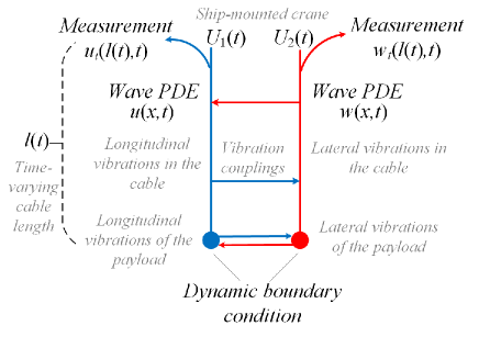
The general plant (27)-(32) whose diagram is shown in Fig.2 covers the vibration dynamics of the DCV (19)-(24) considered in this paper, namely (19)-(24) being a particular case of (27)-(32) by setting the coefficients d1,,d20subscript𝑑1subscript𝑑20d_{1},\ldots,d_{20} as the expressions (222)-(228) in simulation. Moreover, (27)-(32) also can cover the coupled vibration dynamics of mining cable elevators or oil drilling systems.
Refer to caption
Figure 2: Diagram of the plant (27)-(32). The italics text in gray describes the according physical meanings of (27)-(32) in the specific application of the DCV.

Our objective is to exponentially stabilize (27)-(32) through designing control inputs U1(t)subscript𝑈1𝑡U_{1}(t), U2(t)subscript𝑈2𝑡U_{2}(t) in (31)-(32) only using boundary values ut(l(t),t),wt(l(t),t)subscript𝑢𝑡𝑙𝑡𝑡subscript𝑤𝑡𝑙𝑡𝑡u_{t}(l(t),t),w_{t}(l(t),t), i.e., a collocated type output-feedback control system. Note that well-posedness of (27)-(32) can be seen clearly based on an equivalent reformulated plant shown in the next subsection.

II-D Reformulated plant

A preliminary transformation, which allows one to convert the original plant (27)-(32) to a reformulated plant based on which the control design will be conducted, will be utilized in the following.

We introduce a set of Riemann transformations:

z(x,t)=wt(x,t)+d1(x)wx(x,t),𝑧𝑥𝑡subscript𝑤𝑡𝑥𝑡subscript𝑑1𝑥subscript𝑤𝑥𝑥𝑡\displaystyle z(x,t)={w_{t}}(x,t)+\sqrt{{d_{1}}(x)}{w_{x}}(x,t), (34)
v(x,t)=wt(x,t)d1(x)wx(x,t),𝑣𝑥𝑡subscript𝑤𝑡𝑥𝑡subscript𝑑1𝑥subscript𝑤𝑥𝑥𝑡\displaystyle v(x,t)={w_{t}}(x,t)-\sqrt{{d_{1}}(x)}{w_{x}}(x,t), (35)
k(x,t)=ut(x,t)+d6(x)ux(x,t),𝑘𝑥𝑡subscript𝑢𝑡𝑥𝑡subscript𝑑6𝑥subscript𝑢𝑥𝑥𝑡\displaystyle k(x,t)={u_{t}}(x,t)+\sqrt{{d_{6}}(x)}{u_{x}}(x,t), (36)
y(x,t)=ut(x,t)d6(x)ux(x,t)𝑦𝑥𝑡subscript𝑢𝑡𝑥𝑡subscript𝑑6𝑥subscript𝑢𝑥𝑥𝑡\displaystyle y(x,t)={u_{t}}(x,t)-\sqrt{{d_{6}}(x)}{u_{x}}(x,t) (37)

and define new variables as

X(t)=[w(0,t),wt(0,t)],Y(t)=[u(0,t),ut(0,t)],formulae-sequence𝑋𝑡𝑤0𝑡subscript𝑤𝑡0𝑡𝑌𝑡𝑢0𝑡subscript𝑢𝑡0𝑡\displaystyle X(t)=[w(0,t),w_{t}(0,t)],~{}~{}Y(t)=[u(0,t),u_{t}(0,t)], (38)

to reformulate (27)-(32) as

yt(x,t)+d6(x)yx(x,t)=(d7(x)2d1(x)+d9(x)2)z(x,t)subscript𝑦𝑡𝑥𝑡subscript𝑑6𝑥subscript𝑦𝑥𝑥𝑡subscript𝑑7𝑥2subscript𝑑1𝑥subscript𝑑9𝑥2𝑧𝑥𝑡\displaystyle{y_{t}}(x,t)+\sqrt{{d_{6}}(x)}{y_{x}}(x,t)=\left(\frac{{{d_{7}}(x)}}{{2\sqrt{{d_{1}}(x)}}}+\frac{{{d_{9}}(x)}}{2}\right)z(x,t)
+(s1(x)+d10(x)2)k(x,t)+(d9(x)2d7(x)2d1(x))v(x,t)subscript𝑠1𝑥subscript𝑑10𝑥2𝑘𝑥𝑡subscript𝑑9𝑥2subscript𝑑7𝑥2subscript𝑑1𝑥𝑣𝑥𝑡\displaystyle+\left(s_{1}(x)+\frac{{{d_{10}}(x)}}{2}\right)k(x,t)+\left(\frac{{{d_{9}}(x)}}{2}-\frac{{{d_{7}}(x)}}{{2\sqrt{{d_{1}}(x)}}}\right)v(x,t)
+(d10(x)2s1(x))y(x,t),subscript𝑑10𝑥2subscript𝑠1𝑥𝑦𝑥𝑡\displaystyle+\left(\frac{{{d_{10}}(x)}}{2}-s_{1}(x)\right)y(x,t), (39)
kt(x,t)d6(x)kx(x,t)=(d7(x)2d1(x)+d9(x)2)z(x,t)subscript𝑘𝑡𝑥𝑡subscript𝑑6𝑥subscript𝑘𝑥𝑥𝑡subscript𝑑7𝑥2subscript𝑑1𝑥subscript𝑑9𝑥2𝑧𝑥𝑡\displaystyle{k_{t}}(x,t)-\sqrt{{d_{6}}(x)}{k_{x}}(x,t)=\left(\frac{{{d_{7}}(x)}}{{2\sqrt{{d_{1}}(x)}}}+\frac{{{d_{9}}(x)}}{2}\right)z(x,t)
+(s1(x)+d10(x)2)k(x,t)+(d9(x)2d7(x)2d1(x))v(x,t)subscript𝑠1𝑥subscript𝑑10𝑥2𝑘𝑥𝑡subscript𝑑9𝑥2subscript𝑑7𝑥2subscript𝑑1𝑥𝑣𝑥𝑡\displaystyle+\left(s_{1}(x)+\frac{{{d_{10}}(x)}}{2}\right)k(x,t)+\left(\frac{{{d_{9}}(x)}}{2}-\frac{{{d_{7}}(x)}}{{2\sqrt{{d_{1}}(x)}}}\right)v(x,t)
+(d10(x)2s1(x))y(x,t),subscript𝑑10𝑥2subscript𝑠1𝑥𝑦𝑥𝑡\displaystyle+\left(\frac{{{d_{10}}(x)}}{2}-s_{1}(x)\right)y(x,t), (40)
vt(x,t)+d1(x)vx(x,t)=(s2(x)+d4(x)2)z(x,t)subscript𝑣𝑡𝑥𝑡subscript𝑑1𝑥subscript𝑣𝑥𝑥𝑡subscript𝑠2𝑥subscript𝑑4𝑥2𝑧𝑥𝑡\displaystyle{v_{t}}(x,t)+\sqrt{{d_{1}}(x)}{v_{x}}(x,t)=\left(s_{2}(x)+\frac{{{d_{4}}(x)}}{2}\right)z(x,t)
+(d3(x)2d6(x)+d5(x)2)k(x,t)+(d4(x)2s2(x))v(x,t)subscript𝑑3𝑥2subscript𝑑6𝑥subscript𝑑5𝑥2𝑘𝑥𝑡subscript𝑑4𝑥2subscript𝑠2𝑥𝑣𝑥𝑡\displaystyle+\left(\frac{{{d_{3}}(x)}}{{2\sqrt{{d_{6}}(x)}}}+\frac{{{d_{5}}(x)}}{2}\right)k(x,t)+\left(\frac{{{d_{4}}(x)}}{2}-s_{2}(x)\right)v(x,t)
+(d5(x)2d3(x)2d6(x))y(x,t),subscript𝑑5𝑥2subscript𝑑3𝑥2subscript𝑑6𝑥𝑦𝑥𝑡\displaystyle+\left(\frac{{{d_{5}}(x)}}{2}-\frac{{{d_{3}}(x)}}{{2\sqrt{{d_{6}}(x)}}}\right)y(x,t), (41)
zt(x,t)d1(x)zx(x,t)=(s2(x)+d4(x)2)z(x,t)subscript𝑧𝑡𝑥𝑡subscript𝑑1𝑥subscript𝑧𝑥𝑥𝑡subscript𝑠2𝑥subscript𝑑4𝑥2𝑧𝑥𝑡\displaystyle{z_{t}}(x,t)-\sqrt{{d_{1}}(x)}{z_{x}}(x,t)=\left(s_{2}(x)+\frac{{{d_{4}}(x)}}{2}\right)z(x,t)
+(d3(x)2d6(x)+d5(x)2)k(x,t)+(d4(x)2s2(x))v(x,t)subscript𝑑3𝑥2subscript𝑑6𝑥subscript𝑑5𝑥2𝑘𝑥𝑡subscript𝑑4𝑥2subscript𝑠2𝑥𝑣𝑥𝑡\displaystyle+\left(\frac{{{d_{3}}(x)}}{{2\sqrt{{d_{6}}(x)}}}+\frac{{{d_{5}}(x)}}{2}\right)k(x,t)+\left(\frac{{{d_{4}}(x)}}{2}-s_{2}(x)\right)v(x,t)
+(d5(x)2d3(x)2d6(x))y(x,t),subscript𝑑5𝑥2subscript𝑑3𝑥2subscript𝑑6𝑥𝑦𝑥𝑡\displaystyle+\left(\frac{{{d_{5}}(x)}}{2}-\frac{{{d_{3}}(x)}}{{2\sqrt{{d_{6}}(x)}}}\right)y(x,t), (42)
v(0,t)=2C2X(t)z(0,t),𝑣0𝑡2subscript𝐶2𝑋𝑡𝑧0𝑡\displaystyle v(0,t)=2{C_{2}}X(t)-z(0,t), (43)
y(0,t)=2C2Y(t)k(0,t),𝑦0𝑡2subscript𝐶2𝑌𝑡𝑘0𝑡\displaystyle y(0,t)=2{C_{2}}Y(t)-k(0,t), (44)
X˙(t)=(A1B1d12C2d1(0))X(t)˙𝑋𝑡subscript𝐴1subscript𝐵1subscript𝑑12subscript𝐶2subscript𝑑10𝑋𝑡\displaystyle\dot{X}(t)=\left(A_{1}-\frac{{{B_{1}}{d_{12}}C_{2}}}{{\sqrt{{d_{1}}(0)}}}\right)X(t)
+(d13B1C2B1d14C2d6(0))Y(t)subscript𝑑13subscript𝐵1subscript𝐶2subscript𝐵1subscript𝑑14subscript𝐶2subscript𝑑60𝑌𝑡\displaystyle+\left({{d_{13}}}{B_{1}}{C_{2}}-\frac{{{B_{1}}{d_{14}}C_{2}}}{{\sqrt{{d_{6}}(0)}}}\right)Y(t)
+B1d12d1(0)z(0,t)+B1d14d6(0)k(0,t),subscript𝐵1subscript𝑑12subscript𝑑10𝑧0𝑡subscript𝐵1subscript𝑑14subscript𝑑60𝑘0𝑡\displaystyle+\frac{{{B_{1}}{d_{12}}}}{{\sqrt{{d_{1}}(0)}}}z(0,t)+\frac{{{B_{1}}{d_{14}}}}{{\sqrt{{d_{6}}(0)}}}k(0,t), (45)
Y˙(t)=(A2B1d16C2d6(0))Y(t)˙𝑌𝑡subscript𝐴2subscript𝐵1subscript𝑑16subscript𝐶2subscript𝑑60𝑌𝑡\displaystyle\dot{Y}(t)=\left(A_{2}-\frac{{{B_{1}}{d_{16}}C_{2}}}{{\sqrt{{d_{6}}(0)}}}\right)Y(t)
+(d17B1C2B1d18C2d1(0))X(t)subscript𝑑17subscript𝐵1subscript𝐶2subscript𝐵1subscript𝑑18subscript𝐶2subscript𝑑10𝑋𝑡\displaystyle+\left(d_{17}{B_{1}}{C_{2}}-\frac{{{B_{1}}{d_{18}}C_{2}}}{{\sqrt{{d_{1}}(0)}}}\right)X(t)
+B1d18d1(0)z(0,t)+B1d16d6(0)k(0,t),subscript𝐵1subscript𝑑18subscript𝑑10𝑧0𝑡subscript𝐵1subscript𝑑16subscript𝑑60𝑘0𝑡\displaystyle+\frac{{{B_{1}}{d_{18}}}}{{\sqrt{{d_{1}}(0)}}}z(0,t)+\frac{{{B_{1}}{d_{16}}}}{{\sqrt{{d_{6}}(0)}}}k(0,t), (46)
k(l(t),t)=2d6(l(t))d19(l(t))U1(t)+y(l(t),t),𝑘𝑙𝑡𝑡2subscript𝑑6𝑙𝑡subscript𝑑19𝑙𝑡subscript𝑈1𝑡𝑦𝑙𝑡𝑡\displaystyle k(l(t),t)=2\sqrt{{d_{6}}(l(t))}d_{19}(l(t)){U_{1}}(t)+y(l(t),t), (47)
z(l(t),t)=2d1(l(t))d20(l(t))U2(t)+v(l(t),t)𝑧𝑙𝑡𝑡2subscript𝑑1𝑙𝑡subscript𝑑20𝑙𝑡subscript𝑈2𝑡𝑣𝑙𝑡𝑡\displaystyle z(l(t),t)=2\sqrt{{d_{1}}(l(t))}d_{20}(l(t)){U_{2}}(t)+v(l(t),t) (48)

where

s1(x)=d8(x)d6(x)d6(x)2d6(x),subscript𝑠1𝑥subscript𝑑8𝑥subscript𝑑6𝑥superscriptsubscript𝑑6𝑥2subscript𝑑6𝑥\displaystyle s_{1}(x)=\frac{{{d_{8}}(x)-\sqrt{{d_{6}}(x)}{{\sqrt{{d_{6}}(x)}}^{\prime}}}}{{2\sqrt{{d_{6}}(x)}}}, (49)
s2(x)=d2(x)d1(x)d1(x)2d1(x),subscript𝑠2𝑥subscript𝑑2𝑥subscript𝑑1𝑥superscriptsubscript𝑑1𝑥2subscript𝑑1𝑥\displaystyle s_{2}(x)=\frac{{{d_{2}}(x)-\sqrt{{d_{1}}(x)}{{\sqrt{{d_{1}}(x)}}^{\prime}}}}{{2\sqrt{{d_{1}}(x)}}}, (50)

and

A1=[010d11],A2=[010d15],formulae-sequencesubscript𝐴1delimited-[]01missing-subexpressionmissing-subexpressionmissing-subexpressionmissing-subexpressionmissing-subexpressionmissing-subexpressionmissing-subexpressionmissing-subexpressionmissing-subexpressionmissing-subexpressionmissing-subexpressionmissing-subexpressionmissing-subexpressionmissing-subexpressionmissing-subexpressionmissing-subexpressionmissing-subexpressionmissing-subexpression0subscript𝑑11missing-subexpressionmissing-subexpressionmissing-subexpressionmissing-subexpressionmissing-subexpressionmissing-subexpressionmissing-subexpressionmissing-subexpressionmissing-subexpressionmissing-subexpressionmissing-subexpressionmissing-subexpressionmissing-subexpressionmissing-subexpressionmissing-subexpressionmissing-subexpressionmissing-subexpressionmissing-subexpressionsubscript𝐴2delimited-[]01missing-subexpressionmissing-subexpressionmissing-subexpressionmissing-subexpressionmissing-subexpressionmissing-subexpressionmissing-subexpressionmissing-subexpressionmissing-subexpressionmissing-subexpressionmissing-subexpressionmissing-subexpressionmissing-subexpressionmissing-subexpressionmissing-subexpressionmissing-subexpressionmissing-subexpressionmissing-subexpression0subscript𝑑15missing-subexpressionmissing-subexpressionmissing-subexpressionmissing-subexpressionmissing-subexpressionmissing-subexpressionmissing-subexpressionmissing-subexpressionmissing-subexpressionmissing-subexpressionmissing-subexpressionmissing-subexpressionmissing-subexpressionmissing-subexpressionmissing-subexpressionmissing-subexpressionmissing-subexpressionmissing-subexpression\displaystyle A_{1}=\left[{\begin{array}[]{*{20}{c}}0&1\\ 0&{{d_{11}}}\end{array}}\right],A_{2}=\left[{\begin{array}[]{*{20}{c}}0&1\\ 0&{{d_{15}}}\end{array}}\right], (55)
B1=(01),C2=(01).formulae-sequencesubscript𝐵101subscript𝐶201\displaystyle B_{1}=\left(\begin{array}[]{c}0\\ 1\\ \end{array}\right),C_{2}=\left(\begin{array}[]{cc}0&1\\ \end{array}\right). (59)

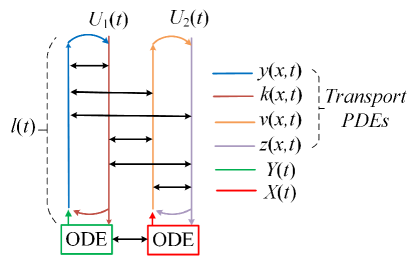
The diagram of the system (39)-(48) is depicted in Fig. 3.

Refer to caption
Figure 3: Diagram of the system (39)-(48).

(39)-(48) is an unstable 4×4444\times 4 coupled linear heterodirectional hyperbolic PDE-ODE system, where y(x,t),v(x,t)𝑦𝑥𝑡𝑣𝑥𝑡y(x,t),v(x,t) and k(x,t),z(x,t)𝑘𝑥𝑡𝑧𝑥𝑡k(x,t),z(x,t) propagate in opposite direction, and the four transport PDEs are coupled with each other in the time-varying spatial domain [0,l(t)]0𝑙𝑡[0,l(t)] and coupled with two ODEs X(t),Y(t)𝑋𝑡𝑌𝑡X(t),Y(t) which are coupled with each other as well at the uncontrolled boundary x=0𝑥0x=0. Compared with our previous result in [34], the two pairs of 2×2222\times 2 coupled linear heterodirectional hyperbolic PDE-ODE system is extended to one 4×4444\times 4 system because additional in-domain couplings between original wave PDEs are considered. Moreover, the assumption that some ODE states at the uncontrolled boundary are measurable [34] is removed in this paper.

In order to rewrite (39)-(48) in a compact form, i.e., in a matrix representation, we define new variables as

p(x,t)𝑝𝑥𝑡\displaystyle p(x,t) =[y(x,t),v(x,t)]T,absentsuperscript𝑦𝑥𝑡𝑣𝑥𝑡𝑇\displaystyle={[y(x,t),v(x,t)]^{T}}, (60)
r(x,t)𝑟𝑥𝑡\displaystyle r(x,t) =[k(x,t),z(x,t)]T,absentsuperscript𝑘𝑥𝑡𝑧𝑥𝑡𝑇\displaystyle={[k(x,t),z(x,t)]^{T}}, (61)
W(t)𝑊𝑡\displaystyle W(t) =[X(t),Y(t)]T.absentsuperscript𝑋𝑡𝑌𝑡𝑇\displaystyle={[X(t),Y(t)]^{T}}. (62)

(39)-(48) can then be rewritten as

pt(x,t)+Q(x)px(x,t)=Ta(x)r(x,t)+Tb(x)p(x,t),subscript𝑝𝑡𝑥𝑡𝑄𝑥subscript𝑝𝑥𝑥𝑡subscript𝑇𝑎𝑥𝑟𝑥𝑡subscript𝑇𝑏𝑥𝑝𝑥𝑡\displaystyle{p_{t}}(x,t)+Q(x){p_{x}}(x,t)={T_{a}}(x)r(x,t)+{T_{b}}(x)p(x,t), (63)
rt(x,t)Q(x)rx(x,t)=Ta(x)r(x,t)+Tb(x)p(x,t),subscript𝑟𝑡𝑥𝑡𝑄𝑥subscript𝑟𝑥𝑥𝑡subscript𝑇𝑎𝑥𝑟𝑥𝑡subscript𝑇𝑏𝑥𝑝𝑥𝑡\displaystyle{r_{t}}(x,t)-Q(x){r_{x}}(x,t)={T_{a}}(x)r(x,t)+{T_{b}}(x)p(x,t), (64)
p(0,t)=C3W(t)r(0,t),𝑝0𝑡subscript𝐶3𝑊𝑡𝑟0𝑡\displaystyle p(0,t)={C_{3}}W(t)-r(0,t), (65)
W˙(t)=(A¯B¯C3)W(t)+2B¯r(0,t),˙𝑊𝑡¯𝐴¯𝐵subscript𝐶3𝑊𝑡2¯𝐵𝑟0𝑡\displaystyle\dot{W}(t)=(\bar{A}-\bar{B}{C_{3}})W(t)+2\bar{B}r(0,t), (66)
r(l(t),t)=R(l(t))U(t)+p(l(t),t)𝑟𝑙𝑡𝑡𝑅𝑙𝑡𝑈𝑡𝑝𝑙𝑡𝑡\displaystyle r(l(t),t)=R(l(t))U(t)+p(l(t),t) (67)

where U(t)=[U1(t),U2(t)]T𝑈𝑡superscriptsubscript𝑈1𝑡subscript𝑈2𝑡𝑇U(t)=[U_{1}(t),U_{2}(t)]^{T}, R(l(t))=2diag(d6(l(t))d19(l(t)),d1(l(t))d20(l(t)))𝑅𝑙𝑡2diagsubscript𝑑6𝑙𝑡subscript𝑑19𝑙𝑡subscript𝑑1𝑙𝑡subscript𝑑20𝑙𝑡R(l(t))=2{\rm{diag}}({{\sqrt{{d_{6}}(l(t))}d_{19}(l(t))}},{{\sqrt{{d_{1}}(l(t))}d_{20}(l(t))}}), Q(x)=diag{Q1(x),Q2(x)}=diag{d6(x),d1(x)}𝑄𝑥diagsubscript𝑄1𝑥subscript𝑄2𝑥diagsubscript𝑑6𝑥subscript𝑑1𝑥Q(x)={\rm{diag}}\{Q_{1}(x),Q_{2}(x)\}={\rm{diag}}\{\sqrt{{d_{6}}(x)},\sqrt{{d_{1}}(x)}\}. A¯,C3,B¯¯𝐴subscript𝐶3¯𝐵\bar{A},{C_{3}},\bar{B} and Ta(x)={Taij(x)}1i,j2subscript𝑇𝑎𝑥subscriptsubscript𝑇𝑎𝑖𝑗𝑥formulae-sequence1𝑖𝑗2{T_{a}}(x)=\{T_{aij}(x)\}_{1\leq i,j\leq 2}, Tb(x)={Tbij(x)}1i,j2subscript𝑇𝑏𝑥subscriptsubscript𝑇𝑏𝑖𝑗𝑥formulae-sequence1𝑖𝑗2{T_{b}}(x)=\{T_{bij}(x)\}_{1\leq i,j\leq 2} are shown as follows

A¯=[A1d13B1C2d17B1C2A2],C3=2[0C2C20],formulae-sequence¯𝐴delimited-[]subscript𝐴1subscript𝑑13subscript𝐵1subscript𝐶2missing-subexpressionmissing-subexpressionmissing-subexpressionmissing-subexpressionmissing-subexpressionmissing-subexpressionmissing-subexpressionmissing-subexpressionmissing-subexpressionmissing-subexpressionmissing-subexpressionmissing-subexpressionmissing-subexpressionmissing-subexpressionmissing-subexpressionmissing-subexpressionmissing-subexpressionmissing-subexpressionsubscript𝑑17subscript𝐵1subscript𝐶2subscript𝐴2missing-subexpressionmissing-subexpressionmissing-subexpressionmissing-subexpressionmissing-subexpressionmissing-subexpressionmissing-subexpressionmissing-subexpressionmissing-subexpressionmissing-subexpressionmissing-subexpressionmissing-subexpressionmissing-subexpressionmissing-subexpressionmissing-subexpressionmissing-subexpressionmissing-subexpressionmissing-subexpressionsubscript𝐶32delimited-[]0subscript𝐶2missing-subexpressionmissing-subexpressionmissing-subexpressionmissing-subexpressionmissing-subexpressionmissing-subexpressionmissing-subexpressionmissing-subexpressionmissing-subexpressionmissing-subexpressionmissing-subexpressionmissing-subexpressionmissing-subexpressionmissing-subexpressionmissing-subexpressionmissing-subexpressionmissing-subexpressionmissing-subexpressionsubscript𝐶20missing-subexpressionmissing-subexpressionmissing-subexpressionmissing-subexpressionmissing-subexpressionmissing-subexpressionmissing-subexpressionmissing-subexpressionmissing-subexpressionmissing-subexpressionmissing-subexpressionmissing-subexpressionmissing-subexpressionmissing-subexpressionmissing-subexpressionmissing-subexpressionmissing-subexpressionmissing-subexpression\displaystyle\bar{A}=\left[{\begin{array}[]{*{20}{c}}{{A_{1}}}&{{{d_{13}}}{B_{1}}{C_{2}}}\\ {{d_{17}}{B_{1}}{C_{2}}}&{{A_{2}}}\end{array}}\right],{C_{3}}=2\left[{\begin{array}[]{*{20}{c}}0&{{C_{2}}}\\ {{C_{2}}}&0\end{array}}\right], (72)
B¯=[B1d142d6(0)B1d122d1(0)B1d162d6(0)B1d182d1(0)]=[00d142d6(0)d122d1(0)00d162d6(0)d182d1(0)]¯𝐵delimited-[]subscript𝐵1subscript𝑑142subscript𝑑60subscript𝐵1subscript𝑑122subscript𝑑10missing-subexpressionmissing-subexpressionmissing-subexpressionmissing-subexpressionmissing-subexpressionmissing-subexpressionmissing-subexpressionmissing-subexpressionmissing-subexpressionmissing-subexpressionmissing-subexpressionmissing-subexpressionmissing-subexpressionmissing-subexpressionmissing-subexpressionmissing-subexpressionmissing-subexpressionmissing-subexpressionsubscript𝐵1subscript𝑑162subscript𝑑60subscript𝐵1subscript𝑑182subscript𝑑10missing-subexpressionmissing-subexpressionmissing-subexpressionmissing-subexpressionmissing-subexpressionmissing-subexpressionmissing-subexpressionmissing-subexpressionmissing-subexpressionmissing-subexpressionmissing-subexpressionmissing-subexpressionmissing-subexpressionmissing-subexpressionmissing-subexpressionmissing-subexpressionmissing-subexpressionmissing-subexpressiondelimited-[]00missing-subexpressionmissing-subexpressionmissing-subexpressionmissing-subexpressionmissing-subexpressionmissing-subexpressionmissing-subexpressionmissing-subexpressionmissing-subexpressionmissing-subexpressionmissing-subexpressionmissing-subexpressionmissing-subexpressionmissing-subexpressionmissing-subexpressionmissing-subexpressionmissing-subexpressionmissing-subexpressionsubscript𝑑142subscript𝑑60subscript𝑑122subscript𝑑10missing-subexpressionmissing-subexpressionmissing-subexpressionmissing-subexpressionmissing-subexpressionmissing-subexpressionmissing-subexpressionmissing-subexpressionmissing-subexpressionmissing-subexpressionmissing-subexpressionmissing-subexpressionmissing-subexpressionmissing-subexpressionmissing-subexpressionmissing-subexpressionmissing-subexpressionmissing-subexpression00missing-subexpressionmissing-subexpressionmissing-subexpressionmissing-subexpressionmissing-subexpressionmissing-subexpressionmissing-subexpressionmissing-subexpressionmissing-subexpressionmissing-subexpressionmissing-subexpressionmissing-subexpressionmissing-subexpressionmissing-subexpressionmissing-subexpressionmissing-subexpressionmissing-subexpressionmissing-subexpressionsubscript𝑑162subscript𝑑60subscript𝑑182subscript𝑑10missing-subexpressionmissing-subexpressionmissing-subexpressionmissing-subexpressionmissing-subexpressionmissing-subexpressionmissing-subexpressionmissing-subexpressionmissing-subexpressionmissing-subexpressionmissing-subexpressionmissing-subexpressionmissing-subexpressionmissing-subexpressionmissing-subexpressionmissing-subexpressionmissing-subexpressionmissing-subexpression\displaystyle\bar{B}=\left[{\begin{array}[]{*{20}{c}}{\frac{{{B_{1}}{d_{14}}}}{{2\sqrt{{d_{6}}(0)}}}}&{\frac{{{B_{1}}{d_{12}}}}{{2\sqrt{{d_{1}}(0)}}}}\\ {\frac{{{B_{1}}{d_{16}}}}{{2\sqrt{{d_{6}}(0)}}}}&{\frac{{{B_{1}}{d_{18}}}}{{2\sqrt{{d_{1}}(0)}}}}\end{array}}\right]=\left[{\begin{array}[]{*{20}{c}}0&0\\ {\frac{{{d_{14}}}}{{2\sqrt{{d_{6}}(0)}}}}&{\frac{{{d_{12}}}}{{2\sqrt{{d_{1}}(0)}}}}\\ 0&0\\ {\frac{{{d_{16}}}}{{2\sqrt{{d_{6}}(0)}}}}&{\frac{{{d_{18}}}}{{2\sqrt{{d_{1}}(0)}}}}\end{array}}\right] (79)
Ta(x)=[s1(x)+d10(x)2d7(x)2d1(x)+d9(x)2d3(x)2d6(x)+d5(x)2s2(x)+d4(x)2],subscript𝑇𝑎𝑥delimited-[]subscript𝑠1𝑥subscript𝑑10𝑥2subscript𝑑7𝑥2subscript𝑑1𝑥subscript𝑑9𝑥2missing-subexpressionmissing-subexpressionmissing-subexpressionmissing-subexpressionmissing-subexpressionmissing-subexpressionmissing-subexpressionmissing-subexpressionmissing-subexpressionmissing-subexpressionmissing-subexpressionmissing-subexpressionmissing-subexpressionmissing-subexpressionmissing-subexpressionmissing-subexpressionmissing-subexpressionmissing-subexpressionsubscript𝑑3𝑥2subscript𝑑6𝑥subscript𝑑5𝑥2subscript𝑠2𝑥subscript𝑑4𝑥2missing-subexpressionmissing-subexpressionmissing-subexpressionmissing-subexpressionmissing-subexpressionmissing-subexpressionmissing-subexpressionmissing-subexpressionmissing-subexpressionmissing-subexpressionmissing-subexpressionmissing-subexpressionmissing-subexpressionmissing-subexpressionmissing-subexpressionmissing-subexpressionmissing-subexpressionmissing-subexpression\displaystyle{T_{a}}(x)=\left[{\begin{array}[]{*{20}{c}}s_{1}(x)+\frac{{d_{10}}(x)}{2}&{\frac{{{d_{7}}(x)}}{{2\sqrt{{d_{1}}(x)}}}+\frac{{d_{9}}(x)}{2}}\\ {\frac{{{d_{3}}(x)}}{{2\sqrt{{d_{6}}(x)}}}+\frac{{d_{5}}(x)}{2}}&{s_{2}(x)+\frac{{d_{4}}(x)}{2}}\end{array}}\right], (82)
Tb(x)=[d10(x)2s1(x)d9(x)2d7(x)2d1(x)d5(x)2d3(x)2d6(x)d4(x)2s2(x)].subscript𝑇𝑏𝑥delimited-[]subscript𝑑10𝑥2subscript𝑠1𝑥subscript𝑑9𝑥2subscript𝑑7𝑥2subscript𝑑1𝑥missing-subexpressionmissing-subexpressionmissing-subexpressionmissing-subexpressionmissing-subexpressionmissing-subexpressionmissing-subexpressionmissing-subexpressionmissing-subexpressionmissing-subexpressionmissing-subexpressionmissing-subexpressionmissing-subexpressionmissing-subexpressionmissing-subexpressionmissing-subexpressionmissing-subexpressionmissing-subexpressionsubscript𝑑5𝑥2subscript𝑑3𝑥2subscript𝑑6𝑥subscript𝑑4𝑥2subscript𝑠2𝑥missing-subexpressionmissing-subexpressionmissing-subexpressionmissing-subexpressionmissing-subexpressionmissing-subexpressionmissing-subexpressionmissing-subexpressionmissing-subexpressionmissing-subexpressionmissing-subexpressionmissing-subexpressionmissing-subexpressionmissing-subexpressionmissing-subexpressionmissing-subexpressionmissing-subexpressionmissing-subexpression\displaystyle{T_{b}}(x)=\left[{\begin{array}[]{*{20}{c}}{\frac{{d_{10}}(x)}{2}-s_{1}(x)}&{\frac{{d_{9}}(x)}{2}-\frac{{{d_{7}}(x)}}{{2\sqrt{{d_{1}}(x)}}}}\\ {\frac{{d_{5}}(x)}{2}-\frac{{{d_{3}}(x)}}{{2\sqrt{{d_{6}}(x)}}}}&{\frac{{d_{4}}(x)}{2}-s_{2}(x)}\end{array}}\right]. (85)

The following assumption is required for the stabilization of the ODE subsystem (66) in the state-feedback and observer design, and is also satisfied in the DCV model by checking the system parameters in the simulation.

Assumption 5.

(A¯B¯C3,B¯)¯𝐴¯𝐵subscript𝐶3¯𝐵(\bar{A}-\bar{B}{C_{3}},\bar{B}) is controllable and (A¯B¯C3,C3)¯𝐴¯𝐵subscript𝐶3subscript𝐶3(\bar{A}-\bar{B}{C_{3}},{C_{3}}) is observable .

Remark 3.

The reformulated plant (63)-(67) obtained from (27)-(32) via the preliminary transformation in Section II-D is well-posed, because it is analogous to the well-posed plant in [23] with setting m=n=2𝑚𝑛2m=n=2, which indicates that the original plant (27)-(32) is also well-posed because of the invertible preliminary transformation.

As compared to [23] where state-feedback control design needing distributed states on a constant PDE domain was presented, in the following sections, we develop an observer-based output-feedback controller upon (63)-(67) on a time-varying PDE domain, and only collocated boundary states are assumed measurable. Then the control input and the stability result will be formulated back in the original plant (27)-(32).

III State-feedback control design

III-A Backstepping design

We seek an invertible transformation that converts the system (63)-(67) (p(x,t),r(x,t),W(t))𝑝𝑥𝑡𝑟𝑥𝑡𝑊𝑡(p(x,t),r(x,t),W(t)) into a so called target system whose exponential stability is obvious.

We postulate the backstepping transformation in the form

α(x,t)𝛼𝑥𝑡\displaystyle\alpha(x,t) =p(x,t)0xK(x,y)p(y,t)𝑑yabsent𝑝𝑥𝑡superscriptsubscript0𝑥𝐾𝑥𝑦𝑝𝑦𝑡differential-d𝑦\displaystyle=p(x,t)-\int_{0}^{x}K(x,y)p(y,t)dy
0xJ(x,y)r(y,t)𝑑yγ(x)W(t),superscriptsubscript0𝑥𝐽𝑥𝑦𝑟𝑦𝑡differential-d𝑦𝛾𝑥𝑊𝑡\displaystyle\quad-\int_{0}^{x}{J(x,y)r(y,t)dy-}\gamma(x)W(t), (86)
β(x,t)𝛽𝑥𝑡\displaystyle\beta(x,t) =r(x,t)0xF(x,y)p(y,t)𝑑yabsent𝑟𝑥𝑡superscriptsubscript0𝑥𝐹𝑥𝑦𝑝𝑦𝑡differential-d𝑦\displaystyle=r(x,t)-\int_{0}^{x}F(x,y)p(y,t)dy
0xN(x,y)r(y,t)𝑑yλ(x)W(t),superscriptsubscript0𝑥𝑁𝑥𝑦𝑟𝑦𝑡differential-d𝑦𝜆𝑥𝑊𝑡\displaystyle\quad-\int_{0}^{x}{N(x,y)r(y,t)dy-}\lambda(x)W(t), (87)

where

K(x,y)={Kij(x,y)}1i,j2,J(x,y)={Jij(x,y)}1i,j2,formulae-sequence𝐾𝑥𝑦subscriptsubscript𝐾𝑖𝑗𝑥𝑦formulae-sequence1𝑖𝑗2𝐽𝑥𝑦subscriptsubscript𝐽𝑖𝑗𝑥𝑦formulae-sequence1𝑖𝑗2\displaystyle K(x,y)=\{K_{ij}(x,y)\}_{1\leq i,j\leq 2},J(x,y)=\{J_{ij}(x,y)\}_{1\leq i,j\leq 2},
F(x,y)={Fij(x,y)}1i,j2,N(x,y)={Nij(x,y)}1i,j2,formulae-sequence𝐹𝑥𝑦subscriptsubscript𝐹𝑖𝑗𝑥𝑦formulae-sequence1𝑖𝑗2𝑁𝑥𝑦subscriptsubscript𝑁𝑖𝑗𝑥𝑦formulae-sequence1𝑖𝑗2\displaystyle F(x,y)=\{F_{ij}(x,y)\}_{1\leq i,j\leq 2},N(x,y)=\{N_{ij}(x,y)\}_{1\leq i,j\leq 2},

on the triangular domain 𝒟={0yxl(t)}𝒟0𝑦𝑥𝑙𝑡\mathcal{D}=\{0\leq y\leq x\leq l(t)\}, and γ(x)={γij(x)}1i2,1j4𝛾𝑥subscriptsubscript𝛾𝑖𝑗𝑥formulae-sequence1𝑖21𝑗4\gamma(x)=\{\gamma_{ij}(x)\}_{1\leq i\leq 2,1\leq j\leq 4}, λ(x)={λij(x)}1i2,1j4𝜆𝑥subscriptsubscript𝜆𝑖𝑗𝑥formulae-sequence1𝑖21𝑗4\lambda(x)=\{\lambda_{ij}(x)\}_{1\leq i\leq 2,1\leq j\leq 4} are to be determined.

The target system (α(x,t),β(x,t),W(t))𝛼𝑥𝑡𝛽𝑥𝑡𝑊𝑡(\alpha(x,t),\beta(x,t),W(t)) is designed as

W˙(t)=A^W(t)+2B¯β(0,t),˙𝑊𝑡^𝐴𝑊𝑡2¯𝐵𝛽0𝑡\displaystyle\dot{W}(t)=\hat{A}W(t)+2\bar{B}\beta(0,t), (88)
αt(x,t)=Q(x)αx(x,t)subscript𝛼𝑡𝑥𝑡𝑄𝑥subscript𝛼𝑥𝑥𝑡\displaystyle{\alpha_{t}}(x,t){\rm{=}}-Q(x){\alpha_{x}}(x,t)
+T¯b(x)α(x,t)+g1(x)β(0,t),subscript¯𝑇𝑏𝑥𝛼𝑥𝑡subscript𝑔1𝑥𝛽0𝑡\displaystyle\quad\quad\quad\quad+{\bar{T}_{b}}(x)\alpha(x,t)+g_{1}(x)\beta(0,t), (89)
βt(x,t)=Q(x)βx(x,t)+T¯a(x)β(x,t)+g(x)β(0,t),subscript𝛽𝑡𝑥𝑡𝑄𝑥subscript𝛽𝑥𝑥𝑡subscript¯𝑇𝑎𝑥𝛽𝑥𝑡𝑔𝑥𝛽0𝑡\displaystyle{\beta_{t}}(x,t)=Q(x){\beta_{x}}(x,t)+{\bar{T}_{a}}(x)\beta(x,t)+g(x)\beta(0,t), (90)
α(0,t)=β(0,t),𝛼0𝑡𝛽0𝑡\displaystyle\alpha(0,t)=-\beta(0,t), (91)
β(l(t),t)=0𝛽𝑙𝑡𝑡0\displaystyle\beta(l(t),t)=0 (92)

where A^=A¯B¯C3+2B¯κ^𝐴¯𝐴¯𝐵subscript𝐶32¯𝐵𝜅\hat{A}=\bar{A}-\bar{B}{C_{3}}+2\bar{B}\kappa is a Hurwitz matrix by choosing κ={κij}1i2,1j4𝜅subscriptsubscript𝜅𝑖𝑗formulae-sequence1𝑖21𝑗4\kappa=\{\kappa_{ij}\}_{1\leq i\leq 2,1\leq j\leq 4} recalling Assumption 5. Note that T¯a(x),T¯b(x)subscript¯𝑇𝑎𝑥subscript¯𝑇𝑏𝑥{\bar{T}_{a}}(x),{\bar{T}_{b}}(x) are diagonal matrices consisting of the diagonal elements of (82)-(85), denoted as T¯a(x)=diag(T¯ai(x))subscript¯𝑇𝑎𝑥diagsubscript¯𝑇𝑎𝑖𝑥{\bar{T}_{a}}(x)={\rm{diag}}({\bar{T}_{ai}}(x)) and T¯b(x)=diag(T¯bi(x))subscript¯𝑇𝑏𝑥diagsubscript¯𝑇𝑏𝑖𝑥{\bar{T}_{b}}(x)={\rm{diag}}({\bar{T}_{bi}}(x)) for i=1,2𝑖12i=1,2. Thus all coupling terms in the PDE domain (63)-(64) are removed. g(x),g1(x)𝑔𝑥subscript𝑔1𝑥g(x),g_{1}(x) are in the form of

g(x)=(00ga(x)0),g1(x)=(00gb(x)0)formulae-sequence𝑔𝑥00subscript𝑔𝑎𝑥0subscript𝑔1𝑥00subscript𝑔𝑏𝑥0\displaystyle g(x)=\left(\begin{array}[]{cc}0&0\\ g_{a}(x)&0\\ \end{array}\right),g_{1}(x)=\left(\begin{array}[]{cc}0&0\\ g_{b}(x)&0\\ \end{array}\right) (97)

where ga(x)=d6(0)F21(x,0)λ22(x)d14d6(0)λ24(x)d16d6(0)+d6(0)N21(x,0)subscript𝑔𝑎𝑥subscript𝑑60subscript𝐹21𝑥0subscript𝜆22𝑥subscript𝑑14subscript𝑑60subscript𝜆24𝑥subscript𝑑16subscript𝑑60subscript𝑑60subscript𝑁21𝑥0g_{a}(x)=\sqrt{{d_{6}}(0)}{F_{21}}(x,0)-\frac{{{{\lambda_{22}}(x)d_{14}}}}{{\sqrt{{d_{6}}(0)}}}-\frac{{{\lambda_{24}}(x){d_{16}}}}{{\sqrt{{d_{6}}(0)}}}+\sqrt{{d_{6}}(0)}{N_{21}}(x,0) and gb(x)=d6(0)J21(x,0)γ22(x)d14d6(0)γ24(x)d16d6(0)+d6(0)K21(x,0)subscript𝑔𝑏𝑥subscript𝑑60subscript𝐽21𝑥0subscript𝛾22𝑥subscript𝑑14subscript𝑑60subscript𝛾24𝑥subscript𝑑16subscript𝑑60subscript𝑑60subscript𝐾21𝑥0g_{b}(x)=\sqrt{{d_{6}}(0)}{J_{21}}(x,0)-\frac{{{\gamma_{22}}(x){d_{14}}}}{{\sqrt{{d_{6}}(0)}}}-\frac{{{\gamma_{24}}(x){d_{16}}}}{{\sqrt{{d_{6}}(0)}}}+\sqrt{{d_{6}}(0)}{K_{21}}(x,0). (88)-(92) is exponentially stable, as we will see in the stability analysis via Lyapunov function in Theorem 1.

By matching the systems (63)-(67) and (88)-(92) through (86)-(87), a lengthy but straightforward calculation leads to the conditions on the kernels in (86)-(87) as follows. F(x,y)𝐹𝑥𝑦F(x,y), N(x,y)𝑁𝑥𝑦N(x,y) λ(x)𝜆𝑥\lambda(x) should satisfy the matrix equations:

Q(x)F(x,x)+F(x,x)Q(x)=Tb(x),𝑄𝑥𝐹𝑥𝑥𝐹𝑥𝑥𝑄𝑥subscript𝑇𝑏𝑥\displaystyle Q(x)F(x,x)+F(x,x)Q(x)=-{T_{b}}(x), (98)
Q(x)N(x,x)N(x,x)Q(x)=T¯a(x)Ta(x),𝑄𝑥𝑁𝑥𝑥𝑁𝑥𝑥𝑄𝑥subscript¯𝑇𝑎𝑥subscript𝑇𝑎𝑥\displaystyle Q(x)N(x,x)-N(x,x)Q(x)=\bar{T}_{a}(x)-T_{a}(x), (99)
N(x,0)Q(0)=F(x,0)Q(0)+2λ(x)B¯+g(x),𝑁𝑥0𝑄0𝐹𝑥0𝑄02𝜆𝑥¯𝐵𝑔𝑥\displaystyle N(x,0)Q(0)=-F(x,0)Q(0)+2\lambda(x)\bar{B}+g(x), (100)
Q(x)Nx(x,y)+Ny(x,y)Q(y)+N(x,y)Q(y)𝑄𝑥subscript𝑁𝑥𝑥𝑦subscript𝑁𝑦𝑥𝑦𝑄𝑦𝑁𝑥𝑦superscript𝑄𝑦\displaystyle Q(x){N_{x}}(x,y)+{N_{y}}(x,y)Q(y)+N(x,y)Q^{\prime}(y)
N(x,y)Ta(y)+T¯a(x)N(x,y)F(x,y)Ta(y)=0,𝑁𝑥𝑦subscript𝑇𝑎𝑦subscript¯𝑇𝑎𝑥𝑁𝑥𝑦𝐹𝑥𝑦subscript𝑇𝑎𝑦0\displaystyle-N(x,y){T_{a}}(y)+{\bar{T}_{a}}(x)N(x,y)-F(x,y){T_{a}}(y)=0, (101)
Q(x)Fx(x,y)Fy(x,y)Q(y)F(x,y)Q(y)𝑄𝑥subscript𝐹𝑥𝑥𝑦subscript𝐹𝑦𝑥𝑦𝑄𝑦𝐹𝑥𝑦superscript𝑄𝑦\displaystyle Q(x){F_{x}}(x,y)-{F_{y}}(x,y)Q(y)-F(x,y)Q^{\prime}(y)
F(x,y)Tb(y)+T¯a(x)F(x,y)N(x,y)Tb(y)=0,𝐹𝑥𝑦subscript𝑇𝑏𝑦subscript¯𝑇𝑎𝑥𝐹𝑥𝑦𝑁𝑥𝑦subscript𝑇𝑏𝑦0\displaystyle-F(x,y){T_{b}}(y)+{\bar{T}_{a}}(x)F(x,y)-N(x,y){T_{b}}(y)=0, (102)
Q(x)λ(x)λ(x)(A¯B¯C3)+T¯a(x)λ(x)𝑄𝑥superscript𝜆𝑥𝜆𝑥¯𝐴¯𝐵subscript𝐶3subscript¯𝑇𝑎𝑥𝜆𝑥\displaystyle Q(x)\lambda^{\prime}(x)-\lambda(x)(\bar{A}-\bar{B}{C_{3}})+{\bar{T}_{a}}(x)\lambda(x)
F(x,0)Q(0)C3+g(x)λ(0)=0,𝐹𝑥0𝑄0subscript𝐶3𝑔𝑥𝜆00\displaystyle-F(x,0)Q(0){C_{3}}+g(x)\lambda(0)=0, (103)
λ(0)=κ𝜆0𝜅\displaystyle\lambda(0)=\kappa (104)

and K(x,y)𝐾𝑥𝑦K(x,y), J(x,y)𝐽𝑥𝑦J(x,y), γ(x)𝛾𝑥\gamma(x) should satisfy

Q(x)J(x,x)J(x,x)Q(x)=Ta(x),𝑄𝑥𝐽𝑥𝑥𝐽𝑥𝑥𝑄𝑥subscript𝑇𝑎𝑥\displaystyle-Q(x)J(x,x)-J(x,x)Q(x)=-{T_{a}}(x), (105)
K(x,x)Q(x)Q(x)K(x,x)=T¯b(x)Tb(x),𝐾𝑥𝑥𝑄𝑥𝑄𝑥𝐾𝑥𝑥subscript¯𝑇𝑏𝑥subscript𝑇𝑏𝑥\displaystyle K(x,x)Q(x)-Q(x)K(x,x)=\bar{T}_{b}(x)-T_{b}(x), (106)
K(x,0)Q(0)=J(x,0)Q(0)+2γ(x)B¯+g1(x),𝐾𝑥0𝑄0𝐽𝑥0𝑄02𝛾𝑥¯𝐵subscript𝑔1𝑥\displaystyle K(x,0)Q(0)=-J(x,0)Q(0)+2\gamma(x)\bar{B}+g_{1}(x), (107)
Q(x)Jx(x,y)+Jy(x,y)Q(y)+J(x,y)Q(y)𝑄𝑥subscript𝐽𝑥𝑥𝑦subscript𝐽𝑦𝑥𝑦𝑄𝑦𝐽𝑥𝑦superscript𝑄𝑦\displaystyle-Q(x){J_{x}}(x,y)+{J_{y}}(x,y)Q(y)+J(x,y)Q^{\prime}(y)
J(x,y)Ta(y)+T¯b(x)J(x,y)K(x,y)Ta(y)=0,𝐽𝑥𝑦subscript𝑇𝑎𝑦subscript¯𝑇𝑏𝑥𝐽𝑥𝑦𝐾𝑥𝑦subscript𝑇𝑎𝑦0\displaystyle-J(x,y){T_{a}}(y)+{\bar{T}_{b}}(x)J(x,y)-K(x,y){T_{a}}(y)=0, (108)
Q(x)Kx(x,y)Ky(x,y)Q(y)K(x,y)Q(y)𝑄𝑥subscript𝐾𝑥𝑥𝑦subscript𝐾𝑦𝑥𝑦𝑄𝑦𝐾𝑥𝑦superscript𝑄𝑦\displaystyle-Q(x){K_{x}}(x,y)-{K_{y}}(x,y)Q(y)-K(x,y)Q^{\prime}(y)
K(x,y)Tb(y)+T¯b(x)K(x,y)J(x,y)Tb(y)=0,𝐾𝑥𝑦subscript𝑇𝑏𝑦subscript¯𝑇𝑏𝑥𝐾𝑥𝑦𝐽𝑥𝑦subscript𝑇𝑏𝑦0\displaystyle-K(x,y){T_{b}}(y)+{\bar{T}_{b}}(x)K(x,y)-J(x,y){T_{b}}(y)=0, (109)
Q(x)γ(x)+γ(x)(A¯B¯C3)+T¯b(x)γ(x)𝑄𝑥superscript𝛾𝑥𝛾𝑥¯𝐴¯𝐵subscript𝐶3subscript¯𝑇𝑏𝑥𝛾𝑥\displaystyle Q(x)\gamma^{\prime}(x)+\gamma(x)(\bar{A}-\bar{B}{C_{3}})+{\bar{T}_{b}}(x)\gamma(x)
K(x,0)Q(0)C3+g1(x)λ(0)=0,𝐾𝑥0𝑄0subscript𝐶3subscript𝑔1𝑥𝜆00\displaystyle-K(x,0)Q(0){C_{3}}+g_{1}(x)\lambda(0)=0, (110)
γ(0)=C3λ(0).𝛾0subscript𝐶3𝜆0\displaystyle\gamma(0)={C_{3}}-\lambda(0). (111)

In order to ensure the existence of a unique solution of the above kernel equations, additional artificial boundary conditions should be imposed, which is shown in the proof of the following lemma about well-posedness of the kernel equations.

Lemma 1.

After adding two additional artificial boundary conditions for the subelements N21,K21subscript𝑁21subscript𝐾21N_{21},K_{21} of kernels N𝑁N and K𝐾K respectively, the matrix equations (98)-(104) have a unique solution F,NL(𝒟)𝐹𝑁superscript𝐿𝒟{F},{N}\in L^{\infty}(\mathcal{D}), λL([0,l(t)])𝜆superscript𝐿0𝑙𝑡\lambda\in L^{\infty}([0,l(t)]) and (105)-(111) have a unique solution K,JL(𝒟)𝐾𝐽superscript𝐿𝒟{K},{J}\in L^{\infty}(\mathcal{D}),γL([0,l(t)])𝛾superscript𝐿0𝑙𝑡\gamma\in L^{\infty}([0,l(t)]).

Proof.

The proof is shown in the Appendix. ∎

With similar derivations, one can show that the inverse transformations are defined as

p(x,t)𝑝𝑥𝑡\displaystyle p(x,t) =α(x,t)0xK¯(x,y)α(y,t)𝑑yabsent𝛼𝑥𝑡superscriptsubscript0𝑥¯𝐾𝑥𝑦𝛼𝑦𝑡differential-d𝑦\displaystyle=\alpha(x,t)-\int_{0}^{x}\bar{K}(x,y)\alpha(y,t)dy
0xJ¯(x,y)β(y,t)𝑑yγ¯(x)W(t),superscriptsubscript0𝑥¯𝐽𝑥𝑦𝛽𝑦𝑡differential-d𝑦¯𝛾𝑥𝑊𝑡\displaystyle-\int_{0}^{x}{\bar{J}(x,y)\beta(y,t)dy-}\bar{\gamma}(x)W(t), (112)
r(x,t)𝑟𝑥𝑡\displaystyle r(x,t) =β(x,t)0xF¯(x,y)α(y,t)𝑑yabsent𝛽𝑥𝑡superscriptsubscript0𝑥¯𝐹𝑥𝑦𝛼𝑦𝑡differential-d𝑦\displaystyle=\beta(x,t)-\int_{0}^{x}\bar{F}(x,y)\alpha(y,t)dy
0xN¯(x,y)β(y,t)𝑑yλ¯(x)W(t),superscriptsubscript0𝑥¯𝑁𝑥𝑦𝛽𝑦𝑡differential-d𝑦¯𝜆𝑥𝑊𝑡\displaystyle-\int_{0}^{x}{\bar{N}(x,y)\beta(y,t)dy-}\bar{\lambda}(x)W(t), (113)

where kernels K¯(x,y),J¯(x,y),γ¯(x),F¯(x,y),N¯(x,y),λ¯(x)¯𝐾𝑥𝑦¯𝐽𝑥𝑦¯𝛾𝑥¯𝐹𝑥𝑦¯𝑁𝑥𝑦¯𝜆𝑥\bar{K}(x,y),\bar{J}(x,y),\bar{\gamma}(x),\bar{F}(x,y),\bar{N}(x,y),\bar{\lambda}(x) can be proved well-posed as Lemma 1.

Once the equation for the kernels are solved, the control input is obtained as

U(t)𝑈𝑡\displaystyle U(t) =R(l(t))1[p(l(t),t)0l(t)F(l(t),y)p(y,t)dy\displaystyle=-R(l(t))^{-1}\bigg{[}p(l(t),t)-\int_{0}^{l(t)}F(l(t),y)p(y,t)dy
0l(t)N(l(t),y)r(y,t)dyλ(l(t))W(t)]\displaystyle-\int_{0}^{l(t)}{N({l(t)},y)r(y,t)dy-}\lambda({l(t)})W(t)\bigg{]} (114)

by matching boundary conditions (67) and (92) via (87).

Applying (34)-(37), (38), (60)-(62), then (114) can be expanded and rewritten as the original states as

U1(t)=subscript𝑈1𝑡absent\displaystyle U_{1}(t)= 1d19(l(t))d6(l(t)[ut(l(t),t)\displaystyle-\frac{1}{d_{19}(l(t))\sqrt{d_{6}(l(t)}}\bigg{[}{u_{t}}(l(t),t)
0l(t)[F11(l(t),y)(ut(y,t)d6(y)ux(y,t))\displaystyle-\int_{0}^{l(t)}\big{[}F_{11}(l(t),y)({u_{t}}(y,t)-\sqrt{{d_{6}}(y)}{u_{x}}(y,t))
+F12(l(t),y)(wt(y,t)d1(y)wx(y,t))]dy\displaystyle+F_{12}(l(t),y)({w_{t}}(y,t)-\sqrt{{d_{1}}(y)}{w_{x}}(y,t))\big{]}dy
0l(t)[N11(l(t),y)(ut(y,t)+d6(y)ux(y,t))\displaystyle-\int_{0}^{l(t)}\big{[}N_{11}(l(t),y)({u_{t}}(y,t)+\sqrt{{d_{6}}(y)}{u_{x}}(y,t))
+N12(l(t),y)(wt(y,t)+d1(y)wx(y,t))]dy\displaystyle+N_{12}(l(t),y)({w_{t}}(y,t)+\sqrt{{d_{1}}(y)}{w_{x}}(y,t))\big{]}dy
λ11(l(t))w(0,t)λ12(l(t))wt(0,t)subscript𝜆11𝑙𝑡𝑤0𝑡subscript𝜆12𝑙𝑡subscript𝑤𝑡0𝑡\displaystyle-\lambda_{11}(l(t))w(0,t)-\lambda_{12}(l(t))w_{t}(0,t)
λ13(l(t))u(0,t)λ14(l(t))ut(0,t)],\displaystyle-\lambda_{13}(l(t))u(0,t)-\lambda_{14}(l(t))u_{t}(0,t)\bigg{]}, (115)
U2(t)=subscript𝑈2𝑡absent\displaystyle U_{2}(t)= 1d20(l(t))d1(l(t)[wt(l(t),t)\displaystyle-\frac{1}{d_{20}(l(t))\sqrt{d_{1}(l(t)}}\bigg{[}{w_{t}}(l(t),t)
0l(t)[F21(l(t),y)(ut(y,t)d6(y)ux(y,t))\displaystyle-\int_{0}^{l(t)}\big{[}F_{21}(l(t),y)({u_{t}}(y,t)-\sqrt{{d_{6}}(y)}{u_{x}}(y,t))
+F22(l(t),y)(wt(y,t)d1(y)wx(y,t))]dy\displaystyle+F_{22}(l(t),y)({w_{t}}(y,t)-\sqrt{{d_{1}}(y)}{w_{x}}(y,t))\big{]}dy
0l(t)[N21(l(t),y)(ut(y,t)+d6(y)ux(y,t))\displaystyle-\int_{0}^{l(t)}\big{[}N_{21}(l(t),y)({u_{t}}(y,t)+\sqrt{{d_{6}}(y)}{u_{x}}(y,t))
+N22(l(t),y)(wt(y,t)+d1(y)wx(y,t))]dy\displaystyle+N_{22}(l(t),y)({w_{t}}(y,t)+\sqrt{{d_{1}}(y)}{w_{x}}(y,t))\big{]}dy
λ21(l(t))w(0,t)λ22(l(t))wt(0,t)subscript𝜆21𝑙𝑡𝑤0𝑡subscript𝜆22𝑙𝑡subscript𝑤𝑡0𝑡\displaystyle-\lambda_{21}(l(t))w(0,t)-\lambda_{22}(l(t))w_{t}(0,t)
λ23(l(t))u(0,t)λ24(l(t))ut(0,t)].\displaystyle-\lambda_{23}(l(t))u(0,t)-\lambda_{24}(l(t))u_{t}(0,t)\bigg{]}. (116)

where inserting (31)-(32) to replace ux(l(t),t)subscript𝑢𝑥𝑙𝑡𝑡u_{x}(l(t),t), wx(l(t),t)subscript𝑤𝑥𝑙𝑡𝑡w_{x}(l(t),t) is used. With the above control laws U1(t),U2(t)subscript𝑈1𝑡subscript𝑈2𝑡U_{1}(t),U_{2}(t), we obtain stability results of the state-feedback closed-loop system, summarized in the following two theorems.

III-B Stability analysis in the state-feedback closed-loop system

III-B1 Stability result of closed-loop system

The exponential stability result of the state-feedback closed-loop system is shown in the following theorem, which physically means the vibration energy of the cable, including kinetic energy and potential energy in two directions, bounded by ξ(wt(,t)2+wx(,t)2+ut(,t)2+ux(,t)2)𝜉superscriptnormsubscript𝑤𝑡𝑡2superscriptnormsubscript𝑤𝑥𝑡2superscriptnormsubscript𝑢𝑡𝑡2superscriptnormsubscript𝑢𝑥𝑡2\xi(\|{{w_{t}}(\cdot,t)}\|^{2}+\|{{w_{x}}(\cdot,t)}\|^{2}+\|{{u_{t}}(\cdot,t)}\|^{2}+\|{{u_{x}}(\cdot,t)}\|^{2}) with ξ>0𝜉0\xi>0, is exponentially convergent to zero, where the decay rate of the vibration energy is adjustable by the control parameters.

Theorem 1.

If initial values (w(x,0),wt(x,0))H2(0,L)×H1(0,L)𝑤𝑥0subscript𝑤𝑡𝑥0superscript𝐻20𝐿superscript𝐻10𝐿(w(x,0),w_{t}(x,0))\in H^{2}(0,L)\times H^{1}(0,L), (u(x,0),ut(x,0))H2(0,L)×H1(0,L)𝑢𝑥0subscript𝑢𝑡𝑥0superscript𝐻20𝐿superscript𝐻10𝐿(u(x,0),u_{t}(x,0))\in H^{2}(0,L)\times H^{1}(0,L), the closed-loop system consisting of the plant (27)-(32) and the state-feedback control law (115)-(116) is exponentially stable in the sense that there exist positive constants Υ1,σ1subscriptΥ1subscript𝜎1\Upsilon_{1},\sigma_{1} such that

((\displaystyle\bigg{(} wt(,t)2+wx(,t)2+ut(,t)2+ux(,t)2superscriptnormsubscript𝑤𝑡𝑡2superscriptnormsubscript𝑤𝑥𝑡2superscriptnormsubscript𝑢𝑡𝑡2superscriptnormsubscript𝑢𝑥𝑡2\displaystyle\|{{w_{t}}(\cdot,t)}\|^{2}+\|{{w_{x}}(\cdot,t)}\|^{2}+\|{{u_{t}}(\cdot,t)}\|^{2}+\|{{u_{x}}(\cdot,t)}\|^{2}
+|w(0,t)|2+|wt(0,t)|2+|u(0,t)|2+|ut(0,t)|2)1/2\displaystyle+|w(0,t)|^{2}+|w_{t}(0,t)|^{2}+|u(0,t)|^{2}+|u_{t}(0,t)|^{2}\bigg{)}^{1/2}
Υ1(wt(,0)2+wx(,0)2+ut(,0)2+ux(,0)2\displaystyle\leq\Upsilon_{1}\bigg{(}\|{{w_{t}}(\cdot,0)}\|^{2}+\|{{w_{x}}(\cdot,0)}\|^{2}+\|{{u_{t}}(\cdot,0)}\|^{2}+\|{{u_{x}}(\cdot,0)}\|^{2}
+|w(0,0)|2+|wt(0,0)|2+|u(0,0)|2+|ut(0,0)|2)1/2eσ1t,\displaystyle+|w(0,0)|^{2}+|w_{t}(0,0)|^{2}+|u(0,0)|^{2}+|u_{t}(0,0)|^{2}\bigg{)}^{1/2}e^{-\sigma_{1}t}, (117)

where u(,t)2superscriptnorm𝑢𝑡2\|u(\cdot,t)\|^{2} is a compact notation for 0l(t)u(x,t)2𝑑xsuperscriptsubscript0𝑙𝑡𝑢superscript𝑥𝑡2differential-d𝑥\int_{0}^{l(t)}{{u}(x,t)^{2}}dx and |||\cdot| denotes the Euclidean norm. The convergence rate σ1subscript𝜎1\sigma_{1} is adjustable by the control parameters.

Proof.

We start from studying the stability of the target system (88)-(92). The equivalent stability property between the target system (88)-(92) and the original system (27)-(32) is ensured via the definitions (34)-(37), (60)-(62) and the backsteppting transformations (86)-(87) and (112)-(113).

Consider the following Lyapunov funtion for the target system (88)-(92),

V1=subscript𝑉1absent\displaystyle V_{1}= WT(t)P1W(t)+120l(t)eδ2xβ(x,t)TRaQ(x)1β(x,t)𝑑xsuperscript𝑊𝑇𝑡subscript𝑃1𝑊𝑡12superscriptsubscript0𝑙𝑡superscript𝑒subscript𝛿2𝑥𝛽superscript𝑥𝑡𝑇subscript𝑅𝑎𝑄superscript𝑥1𝛽𝑥𝑡differential-d𝑥\displaystyle{W^{T}}(t){P_{1}}W(t)+\frac{1}{2}\int_{0}^{l(t)}{{e^{{\delta_{2}}x}}\beta{{(x,t)}^{T}}{R_{a}}Q{{(x)}^{-1}}\beta(x,t)}dx
+120l(t)eδ1xα(x,t)TRbQ(x)1α(x,t)𝑑x,12superscriptsubscript0𝑙𝑡superscript𝑒subscript𝛿1𝑥𝛼superscript𝑥𝑡𝑇subscript𝑅𝑏𝑄superscript𝑥1𝛼𝑥𝑡differential-d𝑥\displaystyle+\frac{1}{2}\int_{0}^{l(t)}{{e^{-{\delta_{1}}x}}\alpha{{(x,t)}^{T}}{R_{b}}Q{{(x)}^{-1}}\alpha(x,t)}dx, (118)

where there exists a positive definite matrix P1=P1Tsubscript𝑃1superscriptsubscript𝑃1𝑇P_{1}={P_{1}^{T}} being the solution to the Lyapunov equation P1A^+A^TP1=Q^1subscript𝑃1^𝐴superscript^𝐴𝑇subscript𝑃1subscript^𝑄1P_{1}\hat{A}+\hat{A}^{T}P_{1}=-\hat{Q}_{1}, for some Q^1=Q^1T>0subscript^𝑄1superscriptsubscript^𝑄1𝑇0\hat{Q}_{1}={{\hat{Q}_{1}}^{T}}>0. Ra,Rbsubscript𝑅𝑎subscript𝑅𝑏R_{a},R_{b} are diagonal matrices as Ra=diag{ra1,ra2}subscript𝑅𝑎diagsubscript𝑟𝑎1subscript𝑟𝑎2R_{a}={\rm diag}\{r_{a1},r_{a2}\}, Rb=diag{rb1,rb2}subscript𝑅𝑏diagsubscript𝑟𝑏1subscript𝑟𝑏2R_{b}={\rm diag}\{r_{b1},r_{b2}\}. The positive parameters ra1,ra2,rb1.rb2,δ1,δ2formulae-sequencesubscript𝑟𝑎1subscript𝑟𝑎2subscript𝑟𝑏1subscript𝑟𝑏2subscript𝛿1subscript𝛿2r_{a1},r_{a2},r_{b1}.r_{b2},\delta_{1},\delta_{2} are to be chosen later.

According to (118), we have

μ1Ω(t)V1(t)μ2Ω(t)subscript𝜇1Ω𝑡subscript𝑉1𝑡subscript𝜇2Ω𝑡\displaystyle\mu_{1}\Omega(t)\leq V_{1}(t)\leq\mu_{2}\Omega(t) (119)

with defining

Ω(t)=|W(t)|2+β(x,t)2+α(x,t)2Ω𝑡superscript𝑊𝑡2superscriptnorm𝛽𝑥𝑡2superscriptnorm𝛼𝑥𝑡2\displaystyle\Omega(t)=|W(t)|^{2}+\|{\beta}{{(x,t)}}\|^{2}+\|{\alpha}{{(x,t)}}\|^{2} (120)

for some positive μ1,μ2subscript𝜇1subscript𝜇2\mu_{1},\mu_{2}. Time derivative of V1(t)subscript𝑉1𝑡V_{1}(t) along (88)-(92) is obtained as

V˙1subscript˙𝑉1\displaystyle\dot{V}_{1} =W˙T(t)P1W(t)+WT(t)P1W˙(t)absentsuperscript˙𝑊𝑇𝑡subscript𝑃1𝑊𝑡superscript𝑊𝑇𝑡subscript𝑃1˙𝑊𝑡\displaystyle={{\dot{W}}^{T}}(t){P_{1}}W(t)+{W^{T}}(t){P_{1}}\dot{W}(t)
+0l(t)eδ2xβ(x,t)TRaQ(x)1βt(x,t)𝑑xsuperscriptsubscript0𝑙𝑡superscript𝑒subscript𝛿2𝑥𝛽superscript𝑥𝑡𝑇subscript𝑅𝑎𝑄superscript𝑥1subscript𝛽𝑡𝑥𝑡differential-d𝑥\displaystyle+\int_{0}^{l(t)}{{e^{{\delta_{2}}x}}\beta{{(x,t)}^{T}}{R_{a}}Q{{(x)}^{-1}}{\beta_{t}}(x,t)}dx
+0l(t)eδ1xα(x,t)TRbQ(x)1αt(x,t)𝑑xsuperscriptsubscript0𝑙𝑡superscript𝑒subscript𝛿1𝑥𝛼superscript𝑥𝑡𝑇subscript𝑅𝑏𝑄superscript𝑥1subscript𝛼𝑡𝑥𝑡differential-d𝑥\displaystyle+\int_{0}^{l(t)}{{e^{-{\delta_{1}}x}}\alpha{{(x,t)}^{T}}{R_{b}}Q{{(x)}^{-1}}{\alpha_{t}}(x,t)}dx
+l˙(t)2eδ1l(t)α(l(t),t)TRbQ(l(t))1α(l(t),t)˙𝑙𝑡2superscript𝑒subscript𝛿1𝑙𝑡𝛼superscript𝑙𝑡𝑡𝑇subscript𝑅𝑏𝑄superscript𝑙𝑡1𝛼𝑙𝑡𝑡\displaystyle+\frac{{\dot{l}(t)}}{2}{e^{-{\delta_{1}}l(t)}}\alpha{(l(t),t)^{T}}{R_{b}}Q{(l(t))^{-1}}\alpha(l(t),t)
=W(t)T(A^TP1+P1A^)W(t)+4WT(t)P1B¯β(0,t)absent𝑊superscript𝑡𝑇superscript^𝐴𝑇subscript𝑃1subscript𝑃1^𝐴𝑊𝑡4superscript𝑊𝑇𝑡subscript𝑃1¯𝐵𝛽0𝑡\displaystyle=W{(t)^{T}}({{\hat{A}}^{T}}{P_{1}}+{P_{1}}\hat{A})W(t)+4{W^{T}}(t){P_{1}}\bar{B}\beta(0,t)
+l˙(t)2eδ1l(t)α(l(t),t)TRbQ(l(t))1α(l(t),t)˙𝑙𝑡2superscript𝑒subscript𝛿1𝑙𝑡𝛼superscript𝑙𝑡𝑡𝑇subscript𝑅𝑏𝑄superscript𝑙𝑡1𝛼𝑙𝑡𝑡\displaystyle+\frac{{\dot{l}(t)}}{2}{e^{-{\delta_{1}}l(t)}}\alpha{(l(t),t)^{T}}{R_{b}}Q{(l(t))^{-1}}\alpha(l(t),t)
+0l(t)eδ2xβ(x,t)TRaQ(x)1T¯a(x)β(x,t)𝑑xsuperscriptsubscript0𝑙𝑡superscript𝑒subscript𝛿2𝑥𝛽superscript𝑥𝑡𝑇subscript𝑅𝑎𝑄superscript𝑥1subscript¯𝑇𝑎𝑥𝛽𝑥𝑡differential-d𝑥\displaystyle+\int_{0}^{l(t)}{{e^{{\delta_{2}}x}}\beta{{(x,t)}^{T}}{R_{a}}Q{{(x)}^{-1}}{{\bar{T}}_{a}}(x)\beta(x,t)}dx
+0l(t)eδ2xβ(x,t)TRaQ(x)1g(x)β(0,t)𝑑xsuperscriptsubscript0𝑙𝑡superscript𝑒subscript𝛿2𝑥𝛽superscript𝑥𝑡𝑇subscript𝑅𝑎𝑄superscript𝑥1𝑔𝑥𝛽0𝑡differential-d𝑥\displaystyle+\int_{0}^{l(t)}{{e^{{\delta_{2}}x}}\beta{{(x,t)}^{T}}{R_{a}}Q{{(x)}^{-1}}g(x)\beta(0,t)}dx
12β(0,t)TRaβ(0,t)δ220l(t)eδ2xβ(x,t)TRaβ(x,t)𝑑x12𝛽superscript0𝑡𝑇subscript𝑅𝑎𝛽0𝑡subscript𝛿22superscriptsubscript0𝑙𝑡superscript𝑒subscript𝛿2𝑥𝛽superscript𝑥𝑡𝑇subscript𝑅𝑎𝛽𝑥𝑡differential-d𝑥\displaystyle-\frac{1}{2}\beta{(0,t)^{T}}{R_{a}}\beta(0,t)-\frac{{{\delta_{2}}}}{2}\int_{0}^{l(t)}{{e^{{\delta_{2}}x}}\beta{{(x,t)}^{T}}{R_{a}}\beta(x,t)}dx
12eδ1l(t)α(l(t),t)TRbα(l(t),t)+12α(0,t)TRbα(0,t)12superscript𝑒subscript𝛿1𝑙𝑡𝛼superscript𝑙𝑡𝑡𝑇subscript𝑅𝑏𝛼𝑙𝑡𝑡12𝛼superscript0𝑡𝑇subscript𝑅𝑏𝛼0𝑡\displaystyle-\frac{1}{2}{e^{-{\delta_{1}}l(t)}}\alpha{(l(t),t)^{T}}{R_{b}}\alpha(l(t),t)+\frac{1}{2}\alpha{(0,t)^{T}}{R_{b}}\alpha(0,t)
δ120l(t)eδ1xα(x,t)TRbα(x,t)𝑑xsubscript𝛿12superscriptsubscript0𝑙𝑡superscript𝑒subscript𝛿1𝑥𝛼superscript𝑥𝑡𝑇subscript𝑅𝑏𝛼𝑥𝑡differential-d𝑥\displaystyle-\frac{{{\delta_{1}}}}{2}\int_{0}^{l(t)}{{e^{-{\delta_{1}}x}}\alpha{{(x,t)}^{T}}{R_{b}}\alpha(x,t)}dx
+0l(t)eδ1xα(x,t)TRbQ(x)1T¯b(x)α(x,t)𝑑xsuperscriptsubscript0𝑙𝑡superscript𝑒subscript𝛿1𝑥𝛼superscript𝑥𝑡𝑇subscript𝑅𝑏𝑄superscript𝑥1subscript¯𝑇𝑏𝑥𝛼𝑥𝑡differential-d𝑥\displaystyle+\int_{0}^{l(t)}{{e^{-{\delta_{1}}x}}\alpha{{(x,t)}^{T}}{R_{b}}Q{{(x)}^{-1}}{{\bar{T}}_{b}}(x)\alpha(x,t)}dx
+0l(t)eδ1xα(x,t)TRbQ(x)1g1(x)β(0,t)𝑑x.superscriptsubscript0𝑙𝑡superscript𝑒subscript𝛿1𝑥𝛼superscript𝑥𝑡𝑇subscript𝑅𝑏𝑄superscript𝑥1subscript𝑔1𝑥𝛽0𝑡differential-d𝑥\displaystyle+\int_{0}^{l(t)}{{e^{-{\delta_{1}}x}}\alpha{{(x,t)}^{T}}{R_{b}}Q{{(x)}^{-1}}{g_{1}}(x)\beta(0,t)}dx. (121)

Applying Young’s inequality and considering the boundedness of the elements 1d1(x),1d6(x),ga(x),gb(x)1subscript𝑑1𝑥1subscript𝑑6𝑥subscript𝑔𝑎𝑥subscript𝑔𝑏𝑥\frac{1}{\sqrt{d_{1}(x)}},\frac{1}{\sqrt{d_{6}(x)}},g_{a}(x),g_{b}(x) in the matrices Q(x)1,g(x),g1(x)𝑄superscript𝑥1𝑔𝑥subscript𝑔1𝑥Q(x)^{-1},g(x),g_{1}(x), there exists ξ>0𝜉0\xi>0 such that the following inequalities holds

0l(t)eδ2xβ(x,t)TRaQ(x)1g(x)β(0,t)𝑑xsuperscriptsubscript0𝑙𝑡superscript𝑒subscript𝛿2𝑥𝛽superscript𝑥𝑡𝑇subscript𝑅𝑎𝑄superscript𝑥1𝑔𝑥𝛽0𝑡differential-d𝑥\displaystyle\quad\int_{0}^{l(t)}{{e^{{\delta_{2}}x}}\beta{{(x,t)}^{T}}{R_{a}}Q{{(x)}^{-1}}g(x)\beta(0,t)}dx
ξ0l(t)eδ2xβ(x,t)TRaβ(x,t)𝑑xabsent𝜉superscriptsubscript0𝑙𝑡superscript𝑒subscript𝛿2𝑥𝛽superscript𝑥𝑡𝑇subscript𝑅𝑎𝛽𝑥𝑡differential-d𝑥\displaystyle\leq\xi\int_{0}^{l(t)}{{e^{{\delta_{2}}x}}\beta{{(x,t)}^{T}}{R_{a}}\beta(x,t)}dx
+ξ0l(t)eδ2Lβ(0,t)TΛaβ(0,t)𝑑x𝜉superscriptsubscript0𝑙𝑡superscript𝑒subscript𝛿2𝐿𝛽superscript0𝑡𝑇subscriptΛ𝑎𝛽0𝑡differential-d𝑥\displaystyle\quad+\xi\int_{0}^{l(t)}{{e^{{\delta_{2}}L}}\beta{{(0,t)}^{T}}{\Lambda_{a}}\beta(0,t)}dx (122)
0l(t)eδ1xα(x,t)TRbQ(x)1g1(x)β(0,t)𝑑xsuperscriptsubscript0𝑙𝑡superscript𝑒subscript𝛿1𝑥𝛼superscript𝑥𝑡𝑇subscript𝑅𝑏𝑄superscript𝑥1subscript𝑔1𝑥𝛽0𝑡differential-d𝑥\displaystyle\quad\int_{0}^{l(t)}{{e^{-{\delta_{1}}x}}\alpha{{(x,t)}^{T}}{R_{b}}Q{{(x)}^{-1}}{g_{1}}(x)\beta(0,t)}dx
ξ0l(t)eδ1xα(x,t)TRbα(x,t)𝑑xabsent𝜉superscriptsubscript0𝑙𝑡superscript𝑒subscript𝛿1𝑥𝛼superscript𝑥𝑡𝑇subscript𝑅𝑏𝛼𝑥𝑡differential-d𝑥\displaystyle\leq\xi\int_{0}^{l(t)}{{e^{-{\delta_{1}}x}}\alpha{{(x,t)}^{T}}{R_{b}}\alpha(x,t)}dx
+ξ0l(t)β(0,t)TΛbβ(0,t)𝑑x,𝜉superscriptsubscript0𝑙𝑡𝛽superscript0𝑡𝑇subscriptΛ𝑏𝛽0𝑡differential-d𝑥\displaystyle\quad+\xi\int_{0}^{l(t)}{\beta{{(0,t)}^{T}}{\Lambda_{b}}\beta(0,t)}dx, (123)

where

Λa=[ra2000],Λb=[rb2000].formulae-sequencesubscriptΛ𝑎delimited-[]subscript𝑟𝑎20missing-subexpressionmissing-subexpressionmissing-subexpressionmissing-subexpressionmissing-subexpressionmissing-subexpressionmissing-subexpressionmissing-subexpressionmissing-subexpressionmissing-subexpressionmissing-subexpressionmissing-subexpressionmissing-subexpressionmissing-subexpressionmissing-subexpressionmissing-subexpressionmissing-subexpressionmissing-subexpression00missing-subexpressionmissing-subexpressionmissing-subexpressionmissing-subexpressionmissing-subexpressionmissing-subexpressionmissing-subexpressionmissing-subexpressionmissing-subexpressionmissing-subexpressionmissing-subexpressionmissing-subexpressionmissing-subexpressionmissing-subexpressionmissing-subexpressionmissing-subexpressionmissing-subexpressionmissing-subexpressionsubscriptΛ𝑏delimited-[]subscript𝑟𝑏20missing-subexpressionmissing-subexpressionmissing-subexpressionmissing-subexpressionmissing-subexpressionmissing-subexpressionmissing-subexpressionmissing-subexpressionmissing-subexpressionmissing-subexpressionmissing-subexpressionmissing-subexpressionmissing-subexpressionmissing-subexpressionmissing-subexpressionmissing-subexpressionmissing-subexpressionmissing-subexpression00missing-subexpressionmissing-subexpressionmissing-subexpressionmissing-subexpressionmissing-subexpressionmissing-subexpressionmissing-subexpressionmissing-subexpressionmissing-subexpressionmissing-subexpressionmissing-subexpressionmissing-subexpressionmissing-subexpressionmissing-subexpressionmissing-subexpressionmissing-subexpressionmissing-subexpressionmissing-subexpression\displaystyle{\Lambda_{a}}=\left[{\begin{array}[]{*{20}{c}}{{r_{a2}}}&0\\ 0&0\end{array}}\right],{\Lambda_{b}}=\left[{\begin{array}[]{*{20}{c}}{{r_{b2}}}&0\\ 0&0\end{array}}\right]. (128)

Inserting (122)-(123) and applying Young’s inequality into (121), one obtains

V˙1(t)12λmin(Q2)|W(t)|2β(0,t)T(Ra2Rb2\displaystyle\dot{V}_{1}(t)\leq-\frac{1}{2}{\lambda_{\min}}({Q_{2}}){\left|{W(t)}\right|^{2}}-\beta{(0,t)^{T}}\bigg{(}\frac{{{R_{a}}}}{2}-\frac{{{R_{b}}}}{2}
8|P1B¯1|2λmin(Q2)I2eδ2LξΛaξΛb)β(0,t)0l(t)eδ2xβ(x,t)T\displaystyle-\frac{{8{{\left|{{P_{1}}{{\bar{B}}_{1}}}\right|}^{2}}}}{{{\lambda_{\min}}({Q_{2}})}}{I_{2}}-{e^{{\delta_{2}}L}}\xi{\Lambda_{a}}-\xi{\Lambda_{b}}\bigg{)}\beta(0,t)-\int_{0}^{l(t)}{e^{{\delta_{2}}x}}\beta{{(x,t)}^{T}}
×Ra((δ22ξ)I2Q(x)1T¯a(x))β(x,t)dx0l(t)eδ1xabsentsubscript𝑅𝑎subscript𝛿22𝜉subscript𝐼2𝑄superscript𝑥1subscript¯𝑇𝑎𝑥𝛽𝑥𝑡𝑑𝑥superscriptsubscript0𝑙𝑡superscript𝑒subscript𝛿1𝑥\displaystyle\times{R_{a}}\left((\frac{{{\delta_{2}}}}{2}-\xi){I_{2}}-Q{{(x)}^{-1}}{{\bar{T}}_{a}}(x)\right)\beta(x,t)dx-\int_{0}^{l(t)}{e^{-{\delta_{1}}x}}
×α(x,t)TRb((δ12ξ)I2Q(x)1T¯b(x))α(x,t)dxabsent𝛼superscript𝑥𝑡𝑇subscript𝑅𝑏subscript𝛿12𝜉subscript𝐼2𝑄superscript𝑥1subscript¯𝑇𝑏𝑥𝛼𝑥𝑡𝑑𝑥\displaystyle\times\alpha{{(x,t)}^{T}}{R_{b}}\left((\frac{{{\delta_{1}}}}{2}-\xi){I_{2}}-Q{{(x)}^{-1}}{{\bar{T}}_{b}}(x)\right)\alpha(x,t)dx
12eδ1l(t)α(l(t),t)TRb(I2Q(l(t))1l˙(t))α(l(t),t),12superscript𝑒subscript𝛿1𝑙𝑡𝛼superscript𝑙𝑡𝑡𝑇subscript𝑅𝑏subscript𝐼2𝑄superscript𝑙𝑡1˙𝑙𝑡𝛼𝑙𝑡𝑡\displaystyle-\frac{1}{2}{e^{-{\delta_{1}}l(t)}}\alpha{(l(t),t)^{T}}{R_{b}}\left({I_{2}}-Q{(l(t))^{-1}}\dot{l}(t)\right)\alpha(l(t),t), (129)

where I2subscript𝐼2I_{2} is a 2×2222\times 2 identity matrix.

The parameters ra1,ra2,rb1.rb2,δ1,δ2formulae-sequencesubscript𝑟𝑎1subscript𝑟𝑎2subscript𝑟𝑏1subscript𝑟𝑏2subscript𝛿1subscript𝛿2r_{a1},r_{a2},r_{b1}.r_{b2},\delta_{1},\delta_{2} are chosen to satisfy

ra1>rb1+16|P1B¯1|2λmin(Q2)+2ra2eδ2Lξ+2rb2ξ,subscript𝑟𝑎1subscript𝑟𝑏116superscriptsubscript𝑃1subscript¯𝐵12subscript𝜆subscript𝑄22subscript𝑟𝑎2superscript𝑒subscript𝛿2𝐿𝜉2subscript𝑟𝑏2𝜉\displaystyle{r_{a1}}>{r_{b1}}+\frac{{16{{\left|{{P_{1}}{{\bar{B}}_{1}}}\right|}^{2}}}}{{{\lambda_{\min}}({Q_{2}})}}+2{r_{a2}}{e^{{\delta_{2}}L}}\xi+2{r_{b2}}\xi, (130)
ra2>rb2+16|P1B¯1|2λmin(Q2)subscript𝑟𝑎2subscript𝑟𝑏216superscriptsubscript𝑃1subscript¯𝐵12subscript𝜆subscript𝑄2\displaystyle{r_{a2}}>{r_{b2}}+\frac{{16{{\left|{{P_{1}}{{\bar{B}}_{1}}}\right|}^{2}}}}{{{\lambda_{\min}}({Q_{2}})}} (131)

with sufficiently large δ1,δ2subscript𝛿1subscript𝛿2\delta_{1},\delta_{2}. Note that positive constants rb1,rb2subscript𝑟𝑏1subscript𝑟𝑏2r_{b1},r_{b2} can be arbitrary. We know the elements in the diagonal matrix Q(l(t))1l˙(t)𝑄superscript𝑙𝑡1˙𝑙𝑡Q{(l(t))^{-1}}\dot{l}(t) is less than 111 by recalling Assumption 4, and the boundedness of all elements in the diagonal matrix Q(x)1𝑄superscript𝑥1Q(x)^{-1}, T¯a(x),T¯b(x)subscript¯𝑇𝑎𝑥subscript¯𝑇𝑏𝑥\bar{T}_{a}(x),\bar{T}_{b}(x) by recalling Assumption 1, we thus arrive at

V˙1(t)η1V1(t),subscript˙𝑉1𝑡subscript𝜂1subscript𝑉1𝑡\displaystyle\dot{V}_{1}(t)\leq-\eta_{1}V_{1}(t), (132)

for some positive η1subscript𝜂1\eta_{1}. It follows that

V1(t)V1(0)eη1tsubscript𝑉1𝑡subscript𝑉10superscript𝑒subscript𝜂1𝑡\displaystyle V_{1}(t)\leq V_{1}(0)e^{-\eta_{1}t} (133)

and then

Ω(t)μ2μ1Ω(0)eη1tΩ𝑡subscript𝜇2subscript𝜇1Ω0superscript𝑒subscript𝜂1𝑡\displaystyle\Omega(t)\leq\frac{\mu_{2}}{\mu_{1}}\Omega(0)e^{-\eta_{1}t} (134)

by recalling (119).

Now we have obtained exponential stability in Ω(t)Ω𝑡\Omega(t). Establishing the relationship between the Ω(t)Ω𝑡\Omega(t) and the appropriate norm of the u(x,t),w(x,t)𝑢𝑥𝑡𝑤𝑥𝑡u(x,t),w(x,t)-system, is the key to establishing exponential stability in the original variables.

Defining

Ξ(t)=ux(,t)2+ut(,t)2+|u(0,t)|2+|ut(0,t)|2Ξ𝑡superscriptnormsubscript𝑢𝑥𝑡2superscriptnormsubscript𝑢𝑡𝑡2superscript𝑢0𝑡2superscriptsubscript𝑢𝑡0𝑡2\displaystyle\Xi(t)=\|u_{x}(\cdot,t)\|^{2}+\|u_{t}(\cdot,t)\|^{2}+|u(0,t)|^{2}+|u_{t}(0,t)|^{2}
+wx(,t)2+wt(,t)2+|w(0,t)|2+|wt(0,t)|2superscriptnormsubscript𝑤𝑥𝑡2superscriptnormsubscript𝑤𝑡𝑡2superscript𝑤0𝑡2superscriptsubscript𝑤𝑡0𝑡2\displaystyle+\|w_{x}(\cdot,t)\|^{2}+\|w_{t}(\cdot,t)\|^{2}+|w(0,t)|^{2}+|w_{t}(0,t)|^{2} (135)

and recalling (34)-(37), (38)-(62), (112)-(113), applying Cauchy-Schwarz inequality, the following inequality holds

θ¯1aΞ(t)Ω(t)θ¯1bΞ(t)subscript¯𝜃1𝑎Ξ𝑡Ω𝑡subscript¯𝜃1𝑏Ξ𝑡\displaystyle{\bar{\theta}_{1a}}\Xi(t)\leq\Omega(t)\leq\bar{\theta}_{1b}\Xi(t) (136)

for some positive θ¯1asubscript¯𝜃1𝑎{\bar{\theta}_{1a}} and θ¯1bsubscript¯𝜃1𝑏\bar{\theta}_{1b}. Therefore, we have

Ξ(t)μ2θ¯1bμ1θ¯1aΞ(0)eη1t.Ξ𝑡subscript𝜇2subscript¯𝜃1𝑏subscript𝜇1subscript¯𝜃1𝑎Ξ0superscript𝑒subscript𝜂1𝑡\displaystyle\Xi(t)\leq\frac{\mu_{2}\bar{\theta}_{1b}}{\mu_{1}\bar{\theta}_{1a}}\Xi(0)e^{-\eta_{1}t}. (137)

Thus (117) is achieved with

Υ1subscriptΥ1\displaystyle\Upsilon_{1} =μ2θ¯1bμ1θ¯1a,σ1=η12,formulae-sequenceabsentsubscript𝜇2subscript¯𝜃1𝑏subscript𝜇1subscript¯𝜃1𝑎subscript𝜎1subscript𝜂12\displaystyle=\sqrt{\frac{\mu_{2}\bar{\theta}_{1b}}{\mu_{1}\bar{\theta}_{1a}}},~{}\sigma_{1}=\frac{\eta_{1}}{2}, (138)

where the convergence rate σ1subscript𝜎1\sigma_{1} can be adjusted by the control parameter κ𝜅\kappa through affecting λmin(Q^1)subscript𝜆subscript^𝑄1{\lambda_{\min}}({\hat{Q}_{1}}). Then the proof of Theorem 1 is completed.∎

III-B2 Exponential convergence of control input

Before proving the exponential convergence of the control input, we propose a lemma first which shows the exponential stability result of the closed-loop system in the sense of H2superscript𝐻2H^{2} norm.

Lemma 2.

For any initial data (w(x,0),wt(x,0))H2(0,L)×H1(0,L)𝑤𝑥0subscript𝑤𝑡𝑥0superscript𝐻20𝐿superscript𝐻10𝐿(w(x,0),w_{t}(x,0))\in H^{2}(0,L)\times H^{1}(0,L), (u(x,0),ut(x,0))H2(0,L)×H1(0,L)𝑢𝑥0subscript𝑢𝑡𝑥0superscript𝐻20𝐿superscript𝐻10𝐿(u(x,0),u_{t}(x,0))\in H^{2}(0,L)\times H^{1}(0,L), the exponential stability estimate of the closed-loop system (u(x,t),w(x,t))𝑢𝑥𝑡𝑤𝑥𝑡(u(x,t),w(x,t)) is obtained in the sense that there exist positive constants Υ1asubscriptΥ1𝑎\Upsilon_{1a} and σ1asubscript𝜎1𝑎\sigma_{1a} such that

(uxx(,t)2+wxx(,t)2+utx(,t)2+wtx(,t)2)12superscriptsuperscriptnormsubscript𝑢𝑥𝑥𝑡2superscriptnormsubscript𝑤𝑥𝑥𝑡2superscriptnormsubscript𝑢𝑡𝑥𝑡2superscriptnormsubscript𝑤𝑡𝑥𝑡212\displaystyle\quad\left(\|u_{xx}(\cdot,t)\|^{2}+\|w_{xx}(\cdot,t)\|^{2}+\|u_{tx}(\cdot,t)\|^{2}+\|w_{tx}(\cdot,t)\|^{2}\right)^{\frac{1}{2}}
Υ1a(ux(,0)2+wx(,0)2+ut(,0)2+wt(,0)2\displaystyle\leq\Upsilon_{1a}\bigg{(}{\|u_{x}(\cdot,0)\|^{2}+\|w_{x}(\cdot,0)\|^{2}+\|u_{t}(\cdot,0)\|^{2}+\|w_{t}(\cdot,0)\|^{2}}
+uxx(,0)2+wxx(,0)2+utx(,0)2+wtx(,0)2superscriptnormsubscript𝑢𝑥𝑥02superscriptnormsubscript𝑤𝑥𝑥02superscriptnormsubscript𝑢𝑡𝑥02superscriptnormsubscript𝑤𝑡𝑥02\displaystyle{+\|u_{xx}(\cdot,0)\|^{2}+\|w_{xx}(\cdot,0)\|^{2}+\|u_{tx}(\cdot,0)\|^{2}+\|w_{tx}(\cdot,0)\|^{2}}
+|w(0,0)|2+|wt(0,0)|2+|u(0,0)|2+|ut(0,0)|2)eσ1at,\displaystyle{+|w(0,0)|^{2}+|w_{t}(0,0)|^{2}+|u(0,0)|^{2}+|u_{t}(0,0)|^{2}}\bigg{)}e^{-\sigma_{1a}t}, (139)
Proof.

Taking the spatial derivative and time derivative of (89)-(90) and (140), (143)-(144) respectively,

W¨(t)=A^W˙(t)+2B¯Q(0)βx(0,t)+2B¯T¯a(0)β(0,t),¨𝑊𝑡^𝐴˙𝑊𝑡2¯𝐵𝑄0subscript𝛽𝑥0𝑡2¯𝐵subscript¯𝑇𝑎0𝛽0𝑡\displaystyle\ddot{W}(t)=\hat{A}\dot{W}(t)+2\bar{B}Q(0){\beta_{x}}(0,t)+2\bar{B}{\bar{T}_{a}}(0)\beta(0,t), (140)
αxt(x,t)=Q(x)αxx(x,t)+(T¯b(x)Q(x))αx(x,t)subscript𝛼𝑥𝑡𝑥𝑡𝑄𝑥subscript𝛼𝑥𝑥𝑥𝑡subscript¯𝑇𝑏𝑥superscript𝑄𝑥subscript𝛼𝑥𝑥𝑡\displaystyle{\alpha_{xt}}(x,t)=-Q(x){\alpha_{xx}}(x,t)+({\bar{T}_{b}}(x)-Q^{\prime}(x))\alpha_{x}(x,t)
+T¯b(x)α(x,t),superscriptsubscript¯𝑇𝑏𝑥𝛼𝑥𝑡\displaystyle\quad\quad\quad\quad\quad+{\bar{T}_{b}}^{\prime}(x)\alpha(x,t), (141)
βxt(x,t)=Q(x)βxx(x,t)+(T¯a(x)+Q(x))βx(x,t)subscript𝛽𝑥𝑡𝑥𝑡𝑄𝑥subscript𝛽𝑥𝑥𝑥𝑡subscript¯𝑇𝑎𝑥superscript𝑄𝑥subscript𝛽𝑥𝑥𝑡\displaystyle{\beta_{xt}}(x,t)=Q(x){\beta_{xx}}(x,t)+({\bar{T}_{a}}(x)+Q^{\prime}(x)){\beta_{x}}(x,t)
+T¯a(x)β(x,t),superscriptsubscript¯𝑇𝑎𝑥𝛽𝑥𝑡\displaystyle\quad\quad\quad\quad\quad+{\bar{T}_{a}}^{\prime}(x)\beta(x,t), (142)
Q(0)αx(0,t)=Q(0)βx(0,t)T¯a(0)β(0,t)𝑄0subscript𝛼𝑥0𝑡𝑄0subscript𝛽𝑥0𝑡subscript¯𝑇𝑎0𝛽0𝑡\displaystyle-Q(0){\alpha_{x}}(0,t)=-Q(0){\beta_{x}}(0,t)-{\bar{T}_{a}}(0)\beta(0,t)
T¯b(0)α(0,t),subscript¯𝑇𝑏0𝛼0𝑡\displaystyle\quad\quad\quad\quad\quad\quad\quad\quad-{\bar{T}_{b}}(0)\alpha(0,t), (143)
βx(l(t),t)=0subscript𝛽𝑥𝑙𝑡𝑡0\displaystyle{\beta}_{x}(l(t),t)=0 (144)

where (90), (92) are used. Note that (144) results from (l˙(t)+Q(l(t)))βx(l(t),t)=0˙𝑙𝑡𝑄𝑙𝑡subscript𝛽𝑥𝑙𝑡𝑡0(\dot{l}(t)+Q(l(t))){\beta_{x}}(l(t),t)=0 where the elements in the diagonal matrix l˙(t)+Q(l(t))˙𝑙𝑡𝑄𝑙𝑡\dot{l}(t)+Q(l(t)) are identically nonzero by recalling Assumption 4. Define new variables ϖ(x,t)=αx(x,t)italic-ϖ𝑥𝑡subscript𝛼𝑥𝑥𝑡\varpi(x,t)=\alpha_{x}(x,t), ζ(x,t)=βx(x,t)𝜁𝑥𝑡subscript𝛽𝑥𝑥𝑡\zeta(x,t)=\beta_{x}(x,t), Z(t)=W˙(t)𝑍𝑡˙𝑊𝑡Z(t)=\dot{W}(t). Consider a Lyapunov function as

V2(t)subscript𝑉2𝑡\displaystyle V_{2}(t) =R1V1(t)+Z(t)TP1Z(t)absentsubscript𝑅1subscript𝑉1𝑡𝑍superscript𝑡𝑇subscript𝑃1𝑍𝑡\displaystyle=R_{1}V_{1}(t)+{{Z}}(t)^{T}P_{1}Z(t)
+120l(t)eδ¯1xζ(x,t)TR¯aQ(x)1ζ(x,t)𝑑x12superscriptsubscript0𝑙𝑡superscript𝑒subscript¯𝛿1𝑥𝜁superscript𝑥𝑡𝑇subscript¯𝑅𝑎𝑄superscript𝑥1𝜁𝑥𝑡differential-d𝑥\displaystyle+\frac{1}{2}\int_{0}^{l(t)}{e^{\bar{\delta}_{1}x}}{\zeta}{{(x,t)}}^{T}\bar{R}_{a}Q(x)^{-1}{\zeta}{{(x,t)}}dx
+120l(t)eδ¯2xϖ(x,t)TR¯bQ(x)1ϖ(x,t)𝑑x,12superscriptsubscript0𝑙𝑡superscript𝑒subscript¯𝛿2𝑥italic-ϖsuperscript𝑥𝑡𝑇subscript¯𝑅𝑏𝑄superscript𝑥1italic-ϖ𝑥𝑡differential-d𝑥\displaystyle+\frac{1}{2}\int_{0}^{l(t)}{e^{-\bar{\delta}_{2}x}}\varpi(x,t)^{T}\bar{R}_{b}Q(x)^{-1}\varpi(x,t)dx, (145)

where R¯a,R¯bsubscript¯𝑅𝑎subscript¯𝑅𝑏\bar{R}_{a},\bar{R}_{b} are diagonal matrices as R¯a=diag{r¯a1,r¯a2}subscript¯𝑅𝑎diagsubscript¯𝑟𝑎1subscript¯𝑟𝑎2\bar{R}_{a}={\rm diag}\{\bar{r}_{a1},\bar{r}_{a2}\}, R¯b=diag{r¯b1,r¯b2}subscript¯𝑅𝑏diagsubscript¯𝑟𝑏1subscript¯𝑟𝑏2\bar{R}_{b}={\rm diag}\{\bar{r}_{b1},\bar{r}_{b2}\}. r¯a1,r¯a2,r¯b1,r¯b2,δ¯1,δ¯1subscript¯𝑟𝑎1subscript¯𝑟𝑎2subscript¯𝑟𝑏1subscript¯𝑟𝑏2subscript¯𝛿1subscript¯𝛿1\bar{r}_{a1},\bar{r}_{a2},\bar{r}_{b1},\bar{r}_{b2},\bar{\delta}_{1},\bar{\delta}_{1} and R1subscript𝑅1R_{1} are positive parameters.

Taking the derivative of (145) along (140)-(144), recalling (129), determining r¯a1,r¯a2,r¯b1,r¯b2,δ¯1,δ¯2subscript¯𝑟𝑎1subscript¯𝑟𝑎2subscript¯𝑟𝑏1subscript¯𝑟𝑏2subscript¯𝛿1subscript¯𝛿2\bar{r}_{a1},\bar{r}_{a2},\bar{r}_{b1},\bar{r}_{b2},\bar{\delta}_{1},\bar{\delta}_{2} through a similar process as (121)-(133), and choosing large enough positive constant R1subscript𝑅1R_{1}, we arrive at

V˙2(t)η2V2(t)subscript˙𝑉2𝑡subscript𝜂2subscript𝑉2𝑡\displaystyle\dot{V}_{2}(t)\leq-\eta_{2}V_{2}(t) (146)

for some positive η2subscript𝜂2\eta_{2}. Recalling backstepping transformations (112)-(113), we have

px(,t)2+rx(,t)2Υ1b(W(0)2+p(,0)2+r(,0)2\displaystyle\|p_{x}(\cdot,t)\|^{2}+\|r_{x}(\cdot,t)\|^{2}\leq\Upsilon_{1b}(W(0)^{2}+\|p(\cdot,0)\|^{2}+\|r(\cdot,0)\|^{2}
+px(,0)2+rx(,0)2)eη2t\displaystyle+\|p_{x}(\cdot,0)\|^{2}+\|r_{x}(\cdot,0)\|^{2})e^{-\eta_{2}t} (147)

for some positive Υ1bsubscriptΥ1𝑏\Upsilon_{1b}. Applying (34)-(37), (60)-(61), the proof of Lemma 2 is completed. ∎

Theorem 2.

In the closed-loop system, the state-feedback controller U1(t)subscript𝑈1𝑡U_{1}(t), U2(t)subscript𝑈2𝑡U_{2}(t) (115)-(116) are bounded and exponentially convergent to zero in the sense that there exist positive constants σ2subscript𝜎2\sigma_{2} and Υ2subscriptΥ2\Upsilon_{2} such that

|U1(t)|2+|U2(t)|2Υ2(ux(,0)2+wx(,0)2\displaystyle|U_{1}(t)|^{2}+|U_{2}(t)|^{2}\leq{\Upsilon_{2}}\bigg{(}\|u_{x}(\cdot,0)\|^{2}+\|w_{x}(\cdot,0)\|^{2}
+ut(,0)2+wt(,0)2+uxx(,0)2+wxx(,0)2superscriptnormsubscript𝑢𝑡02superscriptnormsubscript𝑤𝑡02superscriptnormsubscript𝑢𝑥𝑥02superscriptnormsubscript𝑤𝑥𝑥02\displaystyle+\|u_{t}(\cdot,0)\|^{2}+\|w_{t}(\cdot,0)\|^{2}+\|u_{xx}(\cdot,0)\|^{2}+\|w_{xx}(\cdot,0)\|^{2}
+utx(,0)2+wtx(,0)2+|w(0,0)|2+|wt(0,0)|2superscriptnormsubscript𝑢𝑡𝑥02superscriptnormsubscript𝑤𝑡𝑥02superscript𝑤002superscriptsubscript𝑤𝑡002\displaystyle+\|u_{tx}(\cdot,0)\|^{2}+\|w_{tx}(\cdot,0)\|^{2}+|w(0,0)|^{2}+|w_{t}(0,0)|^{2}
+|u(0,0)|2+|ut(0,0)|2)eσ2t.\displaystyle{+|u(0,0)|^{2}+|u_{t}(0,0)|^{2}}\bigg{)}e^{-{\sigma_{2}}t}. (148)
Proof.

Considering (114) and the exponential stability result in Theorem 1, we know once p(l(t),t)=[ut(l(t),t)d6(l(t))ux(l(t),t)p(l(t),t)=[{u_{t}}(l(t),t)-\sqrt{{d_{6}}(l(t))}{u_{x}}(l(t),t), wt(l(t),t)d1(l(t))wx(l(t),t)]T{w_{t}}(l(t),t)-\sqrt{{d_{1}}(l(t))}{w_{x}}(l(t),t)]^{T} is made sure to be exponentially convergent zero in the sense of |p(l(t),t)|2superscript𝑝𝑙𝑡𝑡2|p(l(t),t)|^{2}, the exponential convergence of the control input is obtained.

Applying Cauchy-Schwarz inequality and recalling (30)-(31), one obtain

|p(l(t),t)|𝑝𝑙𝑡𝑡\displaystyle|p(l(t),t)| 2|p(0,t)|+2Lpx(,t)absent2𝑝0𝑡2𝐿normsubscript𝑝𝑥𝑡\displaystyle\leq 2|p(0,t)|+2\sqrt{L}\|p_{x}(\cdot,t)\|
4|r(0,t)|+4|C3W(t)|+2Lpx(,t)absent4𝑟0𝑡4subscript𝐶3𝑊𝑡2𝐿normsubscript𝑝𝑥𝑡\displaystyle\leq 4|r(0,t)|+4|C_{3}W(t)|+2\sqrt{L}\|p_{x}(\cdot,t)\|
8|r(l(t),t)|+8Lrx(,t)+4|C3W(t)|absent8𝑟𝑙𝑡𝑡8𝐿normsubscript𝑟𝑥𝑡4subscript𝐶3𝑊𝑡\displaystyle\leq 8|r(l(t),t)|+8\sqrt{L}\|r_{x}(\cdot,t)\|+4|C_{3}W(t)|
+2Lpx(,t).2𝐿normsubscript𝑝𝑥𝑡\displaystyle\quad+2\sqrt{L}\|p_{x}(\cdot,t)\|. (149)

Recalling (113), (92) and the exponential convergence of α(,t)2,β(,t)2,|W(t)|2superscriptnorm𝛼𝑡2superscriptnorm𝛽𝑡2superscript𝑊𝑡2\|\alpha(\cdot,t)\|^{2},\|\beta(\cdot,t)\|^{2},|W(t)|^{2} proved in Theorem 1, we have |r(l(t),t)|𝑟𝑙𝑡𝑡|r(l(t),t)| is exponentially convergent to zero. Recalling Lemma 2, we thus have that |p(l(t),t)|𝑝𝑙𝑡𝑡|p(l(t),t)| is exponentially convergent to zero. The proof of Theorem 2 is completed. ∎

IV Observer design

IV-A Observer structure

Consider the sensors only are placed at the actuated boundary, an observer should be designed to estimate the in-domain and uncontrolled boundary states required in the state-feedback control laws (115)-(116). The available measurements are ut(l(t),t)subscript𝑢𝑡𝑙𝑡𝑡u_{t}(l(t),t), wt(l(t),t)subscript𝑤𝑡𝑙𝑡𝑡w_{t}(l(t),t), i.e., p(l(t),t)𝑝𝑙𝑡𝑡p(l(t),t) being known through a convertor as

p(l(t),t)=𝑝𝑙𝑡𝑡absent\displaystyle p(l(t),t)= [ut(l(t),t)d6(l(t))d19(l(t))U1(t),\displaystyle[u_{t}(l(t),t)-\sqrt{d_{6}(l(t))}d_{19}(l(t))U_{1}(t),
wt(l(t),t)d1(l(t))d20(l(t))U2(t)]\displaystyle w_{t}(l(t),t)-\sqrt{d_{1}(l(t))}d_{20}(l(t))U_{2}(t)] (150)

recalling (31)-(32), (60), (34) and (37).

Using the known signal p(l(t),t)𝑝𝑙𝑡𝑡p(l(t),t), the observer for the coupled wave PDE plant (27)-(32) is constructed as:

w^t(x,t)=12(z^(x,t)+v^(x,t)),subscript^𝑤𝑡𝑥𝑡12^𝑧𝑥𝑡^𝑣𝑥𝑡\displaystyle\hat{w}_{t}(x,t)=\frac{1}{2}(\hat{z}(x,t)+\hat{v}(x,t)), (151)
w^x(x,t)=12d1(x)(z^(x,t)v^(x,t)),subscript^𝑤𝑥𝑥𝑡12subscript𝑑1𝑥^𝑧𝑥𝑡^𝑣𝑥𝑡\displaystyle\hat{w}_{x}(x,t)=\frac{1}{2\sqrt{d_{1}(x)}}(\hat{z}(x,t)-\hat{v}(x,t)), (152)
u^t(x,t)=12(k^(x,t)+y^(x,t)),subscript^𝑢𝑡𝑥𝑡12^𝑘𝑥𝑡^𝑦𝑥𝑡\displaystyle\hat{u}_{t}(x,t)=\frac{1}{2}(\hat{k}(x,t)+\hat{y}(x,t)), (153)
u^x(x,t)=12d6(x)(k^(x,t)y^(x,t)),subscript^𝑢𝑥𝑥𝑡12subscript𝑑6𝑥^𝑘𝑥𝑡^𝑦𝑥𝑡\displaystyle\hat{u}_{x}(x,t)=\frac{1}{2\sqrt{d_{6}(x)}}(\hat{k}(x,t)-\hat{y}(x,t)), (154)
p^t(x,t)+Q(x)p^x(x,t)=Ta(x)r^(x,t)+Tb(x)p^(x,t)subscript^𝑝𝑡𝑥𝑡𝑄𝑥subscript^𝑝𝑥𝑥𝑡subscript𝑇𝑎𝑥^𝑟𝑥𝑡subscript𝑇𝑏𝑥^𝑝𝑥𝑡\displaystyle{\hat{p}_{t}}(x,t)+Q(x){\hat{p}_{x}}(x,t)={T_{a}}(x)\hat{r}(x,t)+{T_{b}}(x)\hat{p}(x,t)
+Γ1(x,t)(p(l(t),t)p^(l(t),t)),subscriptΓ1𝑥𝑡𝑝𝑙𝑡𝑡^𝑝𝑙𝑡𝑡\displaystyle+\Gamma_{1}(x,t)(p(l(t),t)-\hat{p}(l(t),t)), (155)
r^t(x,t)Q(x)r^x(x,t)=Ta(x)r^(x,t)+Tb(x)p^(x,t)subscript^𝑟𝑡𝑥𝑡𝑄𝑥subscript^𝑟𝑥𝑥𝑡subscript𝑇𝑎𝑥^𝑟𝑥𝑡subscript𝑇𝑏𝑥^𝑝𝑥𝑡\displaystyle{\hat{r}_{t}}(x,t)-Q(x){\hat{r}_{x}}(x,t)={T_{a}}(x)\hat{r}(x,t)+{T_{b}}(x)\hat{p}(x,t)
+Γ2(x,t)(p(l(t),t)p^(l(t),t)),subscriptΓ2𝑥𝑡𝑝𝑙𝑡𝑡^𝑝𝑙𝑡𝑡\displaystyle+\Gamma_{2}(x,t)(p(l(t),t)-\hat{p}(l(t),t)), (156)
p^(0,t)=C3W^(t)r^(0,t),^𝑝0𝑡subscript𝐶3^𝑊𝑡^𝑟0𝑡\displaystyle\hat{p}(0,t)={C_{3}}\hat{W}(t)-\hat{r}(0,t), (157)
W^˙(t)=(A¯B¯C3)W^(t)+2B¯r^(0,t)˙^𝑊𝑡¯𝐴¯𝐵subscript𝐶3^𝑊𝑡2¯𝐵^𝑟0𝑡\displaystyle\dot{\hat{W}}(t)=(\bar{A}-\bar{B}{C_{3}})\hat{W}(t)+2\bar{B}\hat{r}(0,t)
+Γ3(t)(p(l(t),t)p^(l(t),t)),subscriptΓ3𝑡𝑝𝑙𝑡𝑡^𝑝𝑙𝑡𝑡\displaystyle+\Gamma_{3}(t)(p(l(t),t)-\hat{p}(l(t),t)), (158)
r^(l(t),t)=R(l(t))U(t)+p(l(t),t)^𝑟𝑙𝑡𝑡𝑅𝑙𝑡𝑈𝑡𝑝𝑙𝑡𝑡\displaystyle\hat{r}(l(t),t)=R(l(t))U(t)+p(l(t),t) (159)

where p^=[y^(x,t),v^(x,t)]T^𝑝superscript^𝑦𝑥𝑡^𝑣𝑥𝑡𝑇\hat{p}=[\hat{y}(x,t),\hat{v}(x,t)]^{T}, r^=[k^(x,t),z^(x,t)]T^𝑟superscript^𝑘𝑥𝑡^𝑧𝑥𝑡𝑇\hat{r}=[\hat{k}(x,t),\hat{z}(x,t)]^{T}, W^(t)=[X^(t),Y^(t)]T=[w^(0,t),w^t(0,t),u^(0,t),u^t(0,t)]T^𝑊𝑡superscript^𝑋𝑡^𝑌𝑡𝑇superscript^𝑤0𝑡subscript^𝑤𝑡0𝑡^𝑢0𝑡subscript^𝑢𝑡0𝑡𝑇\hat{W}(t)=[\hat{X}(t),\hat{Y}(t)]^{T}=[\hat{w}(0,t),\hat{w}_{t}(0,t),\hat{u}(0,t),\hat{u}_{t}(0,t)]^{T}.

Note that the observer consists of two parts:

1. (155)-(159) in the sense of a copy of plant (63)-(67) plus output injections is built to estimate p(x,t),r(x,t)𝑝𝑥𝑡𝑟𝑥𝑡p(x,t),r(x,t);

2. Once p(x,t),r(x,t)𝑝𝑥𝑡𝑟𝑥𝑡p(x,t),r(x,t) are estimated successfully by (155)-(159), the estimations of the original plant are straightly obtained as (151)-(154) considering Riemann transformations (34)-(37).

Next, the observer gains Γ1(x,t)subscriptΓ1𝑥𝑡\Gamma_{1}(x,t), Γ2(x,t)subscriptΓ2𝑥𝑡\Gamma_{2}(x,t) and Γ3(t)subscriptΓ3𝑡\Gamma_{3}(t) will be determined to achieve the exponential stability of the observer error system which can be seen in the next subsection. A difference from the traditional ones should be noted that Γ1subscriptΓ1\Gamma_{1}, Γ2subscriptΓ2\Gamma_{2} not only depend on the spatial variable x𝑥x but also depend on time t𝑡t because of the time-varying domain.

IV-B Observer error system

The observation problem is essentially to ensure the observer errors (differences between the estimated and real states) are reduced to zero, by defining adequate observer gains. Denote the observer errors as

w~t(x,t)subscript~𝑤𝑡𝑥𝑡\displaystyle\tilde{w}_{t}(x,t) =wt(x,t)w^t(x,t),absentsubscript𝑤𝑡𝑥𝑡subscript^𝑤𝑡𝑥𝑡\displaystyle=w_{t}(x,t)-\hat{w}_{t}(x,t), (160)
w~x(x,t)subscript~𝑤𝑥𝑥𝑡\displaystyle\tilde{w}_{x}(x,t) =wx(x,t)w^x(x,t),absentsubscript𝑤𝑥𝑥𝑡subscript^𝑤𝑥𝑥𝑡\displaystyle=w_{x}(x,t)-\hat{w}_{x}(x,t), (161)
u~t(x,t)subscript~𝑢𝑡𝑥𝑡\displaystyle\tilde{u}_{t}(x,t) =ut(x,t)u^t(x,t),absentsubscript𝑢𝑡𝑥𝑡subscript^𝑢𝑡𝑥𝑡\displaystyle=u_{t}(x,t)-\hat{u}_{t}(x,t), (162)
u~x(x,t)subscript~𝑢𝑥𝑥𝑡\displaystyle\tilde{u}_{x}(x,t) =ux(x,t)u^x(x,t),absentsubscript𝑢𝑥𝑥𝑡subscript^𝑢𝑥𝑥𝑡\displaystyle=u_{x}(x,t)-\hat{u}_{x}(x,t), (163)
W~(x,t)~𝑊𝑥𝑡\displaystyle\tilde{W}(x,t) =W(x,t)W^(t)absent𝑊𝑥𝑡^𝑊𝑡\displaystyle=W(x,t)-\hat{W}(t)
=[X(t),Y(t)][X^(t),Y^(t)]absent𝑋𝑡𝑌𝑡^𝑋𝑡^𝑌𝑡\displaystyle=[X(t),Y(t)]-[\hat{X}(t),\hat{Y}(t)]
=[w(0,t),wt(0,t),u(0,t),ut(0,t)]Tabsentsuperscript𝑤0𝑡subscript𝑤𝑡0𝑡𝑢0𝑡subscript𝑢𝑡0𝑡𝑇\displaystyle=[w(0,t),w_{t}(0,t),u(0,t),u_{t}(0,t)]^{T}
[w^(0,t),w^t(0,t),u^(0,t),u^t(0,t)]Tsuperscript^𝑤0𝑡subscript^𝑤𝑡0𝑡^𝑢0𝑡subscript^𝑢𝑡0𝑡𝑇\displaystyle\quad-[\hat{w}(0,t),\hat{w}_{t}(0,t),\hat{u}(0,t),\hat{u}_{t}(0,t)]^{T}
=[X~(t),Y~(t)]absent~𝑋𝑡~𝑌𝑡\displaystyle=[\tilde{X}(t),\tilde{Y}(t)]
=[w~(0,t),w~t(0,t),u~(0,t),u~t(0,t)]T,absentsuperscript~𝑤0𝑡subscript~𝑤𝑡0𝑡~𝑢0𝑡subscript~𝑢𝑡0𝑡𝑇\displaystyle=[\tilde{w}(0,t),\tilde{w}_{t}(0,t),\tilde{u}(0,t),\tilde{u}_{t}(0,t)]^{T}, (164)
p~(x,t)~𝑝𝑥𝑡\displaystyle\tilde{p}(x,t) =p(x,t)p^(x,t)=[y~(x,t),v~(x,t)],absent𝑝𝑥𝑡^𝑝𝑥𝑡~𝑦𝑥𝑡~𝑣𝑥𝑡\displaystyle=p(x,t)-\hat{p}(x,t)=[\tilde{y}(x,t),\tilde{v}(x,t)], (165)
r~(x,t)~𝑟𝑥𝑡\displaystyle\tilde{r}(x,t) =r(x,t)r^(x,t)=[k~(x,t),z~(x,t)].absent𝑟𝑥𝑡^𝑟𝑥𝑡~𝑘𝑥𝑡~𝑧𝑥𝑡\displaystyle=r(x,t)-\hat{r}(x,t)=[\tilde{k}(x,t),\tilde{z}(x,t)]. (166)

Recalling (63)-(67), (34)-(37) and (151)-(159), the resulting observer error dynamics is given by

w~t(x,t)=12(z~(x,t)+v~(x,t)),subscript~𝑤𝑡𝑥𝑡12~𝑧𝑥𝑡~𝑣𝑥𝑡\displaystyle\tilde{w}_{t}(x,t)=\frac{1}{2}(\tilde{z}(x,t)+\tilde{v}(x,t)), (167)
w~x(x,t)=12d1(x)(z~(x,t)v~(x,t)),subscript~𝑤𝑥𝑥𝑡12subscript𝑑1𝑥~𝑧𝑥𝑡~𝑣𝑥𝑡\displaystyle\tilde{w}_{x}(x,t)=\frac{1}{2\sqrt{d_{1}(x)}}(\tilde{z}(x,t)-\tilde{v}(x,t)), (168)
u~t(x,t)=12(k~(x,t)+y~(x,t)),subscript~𝑢𝑡𝑥𝑡12~𝑘𝑥𝑡~𝑦𝑥𝑡\displaystyle\tilde{u}_{t}(x,t)=\frac{1}{2}(\tilde{k}(x,t)+\tilde{y}(x,t)), (169)
u~x(x,t)=12d6(x)(k~(x,t)y~(x,t)),subscript~𝑢𝑥𝑥𝑡12subscript𝑑6𝑥~𝑘𝑥𝑡~𝑦𝑥𝑡\displaystyle\tilde{u}_{x}(x,t)=\frac{1}{2\sqrt{d_{6}(x)}}(\tilde{k}(x,t)-\tilde{y}(x,t)), (170)
p~t(x,t)+Q(x)p~x(x,t)=Ta(x)r~(x,t)+Tb(x)p~(x,t)subscript~𝑝𝑡𝑥𝑡𝑄𝑥subscript~𝑝𝑥𝑥𝑡subscript𝑇𝑎𝑥~𝑟𝑥𝑡subscript𝑇𝑏𝑥~𝑝𝑥𝑡\displaystyle{\tilde{p}_{t}}(x,t)+Q(x){\tilde{p}_{x}}(x,t)={T_{a}}(x)\tilde{r}(x,t)+{T_{b}}(x)\tilde{p}(x,t)
+Γ1(x,t)p~(l(t),t),subscriptΓ1𝑥𝑡~𝑝𝑙𝑡𝑡\displaystyle+\Gamma_{1}(x,t)\tilde{p}(l(t),t), (171)
r~t(x,t)Q(x)r~x(x,t)=Ta(x)r~(x,t)+Tb(x)p~(x,t)subscript~𝑟𝑡𝑥𝑡𝑄𝑥subscript~𝑟𝑥𝑥𝑡subscript𝑇𝑎𝑥~𝑟𝑥𝑡subscript𝑇𝑏𝑥~𝑝𝑥𝑡\displaystyle{\tilde{r}_{t}}(x,t)-Q(x){\tilde{r}_{x}}(x,t)={T_{a}}(x)\tilde{r}(x,t)+{T_{b}}(x)\tilde{p}(x,t)
+Γ2(x,t)p~(l(t),t),subscriptΓ2𝑥𝑡~𝑝𝑙𝑡𝑡\displaystyle+\Gamma_{2}(x,t)\tilde{p}(l(t),t), (172)
p~(0,t)=C3W~(t)r~(0,t),~𝑝0𝑡subscript𝐶3~𝑊𝑡~𝑟0𝑡\displaystyle\tilde{p}(0,t)={C_{3}}\tilde{W}(t)-\tilde{r}(0,t), (173)
W~˙(t)=(A¯B¯C3)W~(t)+2B¯r~(0,t)˙~𝑊𝑡¯𝐴¯𝐵subscript𝐶3~𝑊𝑡2¯𝐵~𝑟0𝑡\displaystyle\dot{\tilde{W}}(t)=(\bar{A}-\bar{B}{C_{3}})\tilde{W}(t)+2\bar{B}\tilde{r}(0,t)
+Γ3(t)p~(l(t),t),subscriptΓ3𝑡~𝑝𝑙𝑡𝑡\displaystyle+\Gamma_{3}(t)\tilde{p}(l(t),t), (174)
r~(l(t),t)=0,~𝑟𝑙𝑡𝑡0\displaystyle\tilde{r}(l(t),t)=0, (175)

where the subsystem (171)-(175) describing dynamics of the observer error of the system (63)-(67), determines the observer error of the plant (27)-(32) via (167)-(170). Therefore, the exponential stability of (171)-(175) is the core to make sure the proposed observer can be exponentially convergent to the actual states of the original plant (27)-(32).

IV-C Observer backtepping design

To find the observer gains Γ1(x,t),Γ2(x,t),Γ3(t)subscriptΓ1𝑥𝑡subscriptΓ2𝑥𝑡subscriptΓ3𝑡\Gamma_{1}(x,t),\Gamma_{2}(x,t),\Gamma_{3}(t) that guarantee that (171)-(175) is exponentially stable, we use a transformation to map (171)-(175) to a target observer error system whose exponential stability result is straightforward to obtain.

The transformation is introduced as

p~(x,t)=~𝑝𝑥𝑡absent\displaystyle\tilde{p}(x,t)= α~(x,t)xl(t)φ¯(x,y)α~(y,t)𝑑y,~𝛼𝑥𝑡superscriptsubscript𝑥𝑙𝑡¯𝜑𝑥𝑦~𝛼𝑦𝑡differential-d𝑦\displaystyle\tilde{\alpha}(x,t)-\int_{x}^{l(t)}\bar{\varphi}(x,y)\tilde{\alpha}(y,t)dy, (176)
r~(x,t)=~𝑟𝑥𝑡absent\displaystyle\tilde{r}(x,t)= β~(x,t)xl(t)ψ¯(x,y)α~(y,t)𝑑y,~𝛽𝑥𝑡superscriptsubscript𝑥𝑙𝑡¯𝜓𝑥𝑦~𝛼𝑦𝑡differential-d𝑦\displaystyle\tilde{\beta}(x,t)-\int_{x}^{l(t)}\bar{\psi}(x,y)\tilde{\alpha}(y,t)dy, (177)
W~(t)=~𝑊𝑡absent\displaystyle\tilde{W}(t)= S~(t)+0l(t)K¯(y)α~(y,t)𝑑y,~𝑆𝑡superscriptsubscript0𝑙𝑡¯𝐾𝑦~𝛼𝑦𝑡differential-d𝑦\displaystyle\tilde{S}(t)+\int_{0}^{l(t)}{\bar{K}(y)\tilde{\alpha}(y,t)}dy, (178)

where kernels φ¯(x,y)={φ¯ij(x,y)}1i,j2¯𝜑𝑥𝑦subscriptsubscript¯𝜑𝑖𝑗𝑥𝑦formulae-sequence1𝑖𝑗2\bar{\varphi}(x,y)=\{\bar{\varphi}_{ij}(x,y)\}_{1\leq i,j\leq 2}, ψ¯(x,y)={ψ¯ij(x,y)}1i,j2¯𝜓𝑥𝑦subscriptsubscript¯𝜓𝑖𝑗𝑥𝑦formulae-sequence1𝑖𝑗2\bar{\psi}(x,y)=\{\bar{\psi}_{ij}(x,y)\}_{1\leq i,j\leq 2} on a triangular domain 𝒟1={0xyl(t)}subscript𝒟10𝑥𝑦𝑙𝑡\mathcal{D}_{1}=\{0\leq x\leq y\leq l(t)\} and K¯(y)={K¯ij(y)}1i4,1j2¯𝐾𝑦subscriptsubscript¯𝐾𝑖𝑗𝑦formulae-sequence1𝑖41𝑗2\bar{K}(y)=\{\bar{K}_{ij}(y)\}_{1\leq i\leq 4,1\leq j\leq 2} are to be determined.

The target observer error system is set up as

α~t(x,t)+Q(x)α~x(x,t)=Ta(x)β~(x,t)+T¯b(x)α~(x,t)subscript~𝛼𝑡𝑥𝑡𝑄𝑥subscript~𝛼𝑥𝑥𝑡subscript𝑇𝑎𝑥~𝛽𝑥𝑡subscript¯𝑇𝑏𝑥~𝛼𝑥𝑡\displaystyle{{\tilde{\alpha}}_{t}}(x,t)+Q(x){{\tilde{\alpha}}_{x}}(x,t)={{T}_{a}}(x)\tilde{\beta}(x,t)+{{\bar{T}}_{b}}(x)\tilde{\alpha}(x,t)
+xl(t)M¯(x,y)β~(y,t)𝑑y,superscriptsubscript𝑥𝑙𝑡¯𝑀𝑥𝑦~𝛽𝑦𝑡differential-d𝑦\displaystyle+\int_{x}^{l(t)}{\bar{M}(x,y)}\tilde{\beta}(y,t)dy, (179)
β~t(x,t)Q(x)β~x(x,t)=xl(t)N¯(x,y)β~(y,t)𝑑ysubscript~𝛽𝑡𝑥𝑡𝑄𝑥subscript~𝛽𝑥𝑥𝑡superscriptsubscript𝑥𝑙𝑡¯𝑁𝑥𝑦~𝛽𝑦𝑡differential-d𝑦\displaystyle{{\tilde{\beta}}_{t}}(x,t)-Q(x){{\tilde{\beta}}_{x}}(x,t)=\int_{x}^{l(t)}{\bar{N}(x,y)}\tilde{\beta}(y,t)dy
+Ta(x)β~(x,t),subscript𝑇𝑎𝑥~𝛽𝑥𝑡\displaystyle+T_{a}(x)\tilde{\beta}(x,t), (180)
α~(0,t)=C3S~(t)β~(0,t)+0l(t)H(y)α~(y,t)𝑑y,~𝛼0𝑡subscript𝐶3~𝑆𝑡~𝛽0𝑡superscriptsubscript0𝑙𝑡𝐻𝑦~𝛼𝑦𝑡differential-d𝑦\displaystyle\tilde{\alpha}(0,t)={C_{3}}\tilde{S}(t)-\tilde{\beta}(0,t)+\int_{0}^{l(t)}{H(y)\tilde{\alpha}(y,t)}dy, (181)
β~(l(t),t)=0,~𝛽𝑙𝑡𝑡0\displaystyle\tilde{\beta}(l(t),t)=0, (182)
S~˙(t)=AˇS~(t)+Eˇβ~(0,t)+0l(t)G(y)β~(y,t)𝑑y˙~𝑆𝑡ˇ𝐴~𝑆𝑡ˇ𝐸~𝛽0𝑡superscriptsubscript0𝑙𝑡𝐺𝑦~𝛽𝑦𝑡differential-d𝑦\displaystyle\dot{\tilde{S}}(t)=\check{A}\tilde{S}(t)+\check{E}\tilde{\beta}(0,t)+\int_{0}^{l(t)}G(y)\tilde{\beta}(y,t)dy (183)

where Aˇ=A¯B¯C3L0C3ˇ𝐴¯𝐴¯𝐵subscript𝐶3subscript𝐿0subscript𝐶3\check{A}=\bar{A}-\bar{B}{C_{3}}-{L_{0}}{C_{3}} is a Hurwitz matrix by choosing L0={L0ij}1i4,1j2subscript𝐿0subscriptsubscript𝐿0𝑖𝑗formulae-sequence1𝑖41𝑗2L_{0}=\{L_{0ij}\}_{1\leq i\leq 4,1\leq j\leq 2} recalling Assumption 5, and M¯(x,y)¯𝑀𝑥𝑦{\bar{M}(x,y)}, N¯(x,y)¯𝑁𝑥𝑦\bar{N}(x,y) satisfy

M¯(x,y)=xyφ¯(x,z)M¯(z,y)𝑑z+φ¯(x,y)Ta(y),¯𝑀𝑥𝑦superscriptsubscript𝑥𝑦¯𝜑𝑥𝑧¯𝑀𝑧𝑦differential-d𝑧¯𝜑𝑥𝑦subscript𝑇𝑎𝑦\displaystyle\bar{M}(x,y){\rm{=}}\int_{x}^{y}{\bar{\varphi}(x,z)\bar{M}(z,y)}dz+\bar{\varphi}(x,y){T_{a}}(y), (184)
N¯(x,y)=xyψ¯(x,z)M¯(z,y)𝑑z+ψ¯(x,y)Ta(y).¯𝑁𝑥𝑦superscriptsubscript𝑥𝑦¯𝜓𝑥𝑧¯𝑀𝑧𝑦differential-d𝑧¯𝜓𝑥𝑦subscript𝑇𝑎𝑦\displaystyle\bar{N}(x,y){\rm{=}}\int_{x}^{y}{\bar{\psi}(x,z)\bar{M}(z,y)}dz+\bar{\psi}(x,y){T_{a}}(y). (185)

Note that H(y)={hij(y)}1i,j2𝐻𝑦subscriptsubscript𝑖𝑗𝑦formulae-sequence1𝑖𝑗2H(y)=\{h_{ij}(y)\}_{1\leq i,j\leq 2} in (181) is a strict lower triangular matrix as

H(y)=(00ψ¯2,1(0,y)+φ¯2,1(0,y)+K¯21(y)0),𝐻𝑦00subscript¯𝜓210𝑦subscript¯𝜑210𝑦subscript¯𝐾21𝑦0\displaystyle H(y)=\left(\begin{array}[]{cc}0&0\\ \bar{\psi}_{2,1}(0,y)+\bar{\varphi}_{2,1}(0,y)+\bar{K}_{21}(y)&0\\ \end{array}\right), (188)

and G(y)={Gij(y)}1i4,1j2,Eˇ={Eˇij}1i4,1j2formulae-sequence𝐺𝑦subscriptsubscript𝐺𝑖𝑗𝑦formulae-sequence1𝑖41𝑗2ˇ𝐸subscriptsubscriptˇ𝐸𝑖𝑗formulae-sequence1𝑖41𝑗2G(y)=\{G_{ij}(y)\}_{1\leq i\leq 4,1\leq j\leq 2},\check{E}=\{\check{E}_{ij}\}_{1\leq i\leq 4,1\leq j\leq 2} in (183) are equal to K¯(0,y)T¯a(y)0yK¯(0,z)M¯(z,y)𝑑z¯𝐾0𝑦subscript¯𝑇𝑎𝑦superscriptsubscript0𝑦¯𝐾0𝑧¯𝑀𝑧𝑦differential-d𝑧-\bar{K}(0,y){{\bar{T}}_{a}}(y)-\int_{0}^{y}{\bar{K}(0,z)\bar{M}(z,y)dz} and L0+2B¯subscript𝐿02¯𝐵L_{0}+2\bar{B} respectively. The exponential stability of the target system (179)-(183) will be seen in Lemma 4.

By matching (171)-(175) and (179)-(183) through the transformation (176)-(178), the conditions on the kernels in (176)-(178) and observer gains in (155), (156), (158) are obtained as follows. Kernels φ¯(x,y)¯𝜑𝑥𝑦\bar{\varphi}(x,y), ψ¯(x,y)¯𝜓𝑥𝑦\bar{\psi}(x,y), K¯(y)¯𝐾𝑦\bar{K}(y) should satisfy the matrix equations:

φ¯y(x,y)Q(y)Q(x)φ¯x(x,y)φ¯(x,y)Q(y)subscript¯𝜑𝑦𝑥𝑦𝑄𝑦𝑄𝑥subscript¯𝜑𝑥𝑥𝑦¯𝜑𝑥𝑦superscript𝑄𝑦\displaystyle-{{\bar{\varphi}}_{y}}(x,y)Q(y)-Q(x){{\bar{\varphi}}_{x}}(x,y)-\bar{\varphi}(x,y)Q^{\prime}(y)
+Ta(x)ψ¯(x,y)+Tb(x)φ¯(x,y)φ¯(x,y)T¯b(y)=0,subscript𝑇𝑎𝑥¯𝜓𝑥𝑦subscript𝑇𝑏𝑥¯𝜑𝑥𝑦¯𝜑𝑥𝑦subscript¯𝑇𝑏𝑦0\displaystyle+{T_{a}}(x)\bar{\psi}(x,y)+{T_{b}}(x)\bar{\varphi}(x,y)-\bar{\varphi}(x,y){{\bar{T}}_{b}}(y)=0, (189)
ψ¯y(x,y)Q(y)+Q(x)ψ¯x(x,y)ψ¯(x,y)Q(y)subscript¯𝜓𝑦𝑥𝑦𝑄𝑦𝑄𝑥subscript¯𝜓𝑥𝑥𝑦¯𝜓𝑥𝑦superscript𝑄𝑦\displaystyle-{{\bar{\psi}}_{y}}(x,y)Q(y)+Q(x){{\bar{\psi}}_{x}}(x,y)-\bar{\psi}(x,y)Q^{\prime}(y)
+Ta(x)ψ¯(x,y)ψ¯(x,y)T¯b(y)+Tb(x)φ¯(x,y)=0,subscript𝑇𝑎𝑥¯𝜓𝑥𝑦¯𝜓𝑥𝑦subscript¯𝑇𝑏𝑦subscript𝑇𝑏𝑥¯𝜑𝑥𝑦0\displaystyle+{T_{a}}(x)\bar{\psi}(x,y)-\bar{\psi}(x,y){{\bar{T}}_{b}}(y)+{T_{b}}(x)\bar{\varphi}(x,y)=0, (190)
Q(x)φ¯(x,x)φ¯(x,x)Q(x)=Tb(x)T¯b(x),𝑄𝑥¯𝜑𝑥𝑥¯𝜑𝑥𝑥𝑄𝑥subscript𝑇𝑏𝑥subscript¯𝑇𝑏𝑥\displaystyle Q(x)\bar{\varphi}(x,x)-\bar{\varphi}(x,x)Q(x)={T_{b}}(x)-{{\bar{T}}_{b}}(x), (191)
Q(x)ψ¯(x,x)+ψ¯(x,x)Q(x)=Tb(x),𝑄𝑥¯𝜓𝑥𝑥¯𝜓𝑥𝑥𝑄𝑥subscript𝑇𝑏𝑥\displaystyle Q(x)\bar{\psi}(x,x)+\bar{\psi}(x,x)Q(x){\rm{=}}-{T_{b}}(x), (192)
ψ¯(0,y)+φ¯(0,y)+C3K¯(y)=H(y),¯𝜓0𝑦¯𝜑0𝑦subscript𝐶3¯𝐾𝑦𝐻𝑦\displaystyle\bar{\psi}(0,y)+\bar{\varphi}(0,y)+C_{3}\bar{K}(y)=H(y), (193)
K¯(y)Q(y)+(A¯B¯C3L0C3)K¯(y)superscript¯𝐾𝑦𝑄𝑦¯𝐴¯𝐵subscript𝐶3subscript𝐿0subscript𝐶3¯𝐾𝑦\displaystyle-\bar{K}^{\prime}(y)Q(y)+(\bar{A}-\bar{B}{C_{3}}-{L_{0}}{C_{3}})\bar{K}(y)
K¯(y)[Q(y)+T¯b(y)]¯𝐾𝑦delimited-[]superscript𝑄𝑦subscript¯𝑇𝑏𝑦\displaystyle-\bar{K}(y)[Q^{\prime}(y)+{{\bar{T}}_{b}}(y)]
L0φ¯(0,y)(2B¯+L0)ψ¯(0,y)=0,subscript𝐿0¯𝜑0𝑦2¯𝐵subscript𝐿0¯𝜓0𝑦0\displaystyle-{L_{0}}\bar{\varphi}(0,y)-(2\bar{B}+{L_{0}})\bar{\psi}(0,y)=0, (194)
K¯(0)=L0Q(0)1¯𝐾0subscript𝐿0𝑄superscript01\displaystyle\bar{K}(0)={L_{0}}Q{(0)^{-1}} (195)

and the observe gains are obtained as

Γ1(x,t)subscriptΓ1𝑥𝑡\displaystyle{\Gamma_{1}}(x,t) =l˙(t)φ¯(x,l(t))φ¯(x,l(t))Q(l(t)),absent˙𝑙𝑡¯𝜑𝑥𝑙𝑡¯𝜑𝑥𝑙𝑡𝑄𝑙𝑡\displaystyle=\dot{l}(t)\bar{\varphi}(x,l(t))-\bar{\varphi}(x,l(t))Q(l(t)), (196)
Γ2(x,t)subscriptΓ2𝑥𝑡\displaystyle{\Gamma_{2}}(x,t) =l˙(t)ψ¯(x,l(t))ψ¯(x,l(t))Q(l(t)),absent˙𝑙𝑡¯𝜓𝑥𝑙𝑡¯𝜓𝑥𝑙𝑡𝑄𝑙𝑡\displaystyle=\dot{l}(t)\bar{\psi}(x,l(t))-\bar{\psi}(x,l(t))Q(l(t)), (197)
Γ3(t)subscriptΓ3𝑡\displaystyle{\Gamma_{3}}(t) =l˙(t)K¯(l(t))K¯(l(t))Q(l(t)).absent˙𝑙𝑡¯𝐾𝑙𝑡¯𝐾𝑙𝑡𝑄𝑙𝑡\displaystyle=\dot{l}(t)\bar{K}(l(t))-\bar{K}(l(t))Q(l(t)). (198)
Lemma 3.

After adding an additional artificial boundary condition for the element φ¯21subscript¯𝜑21\bar{\varphi}_{21} in the matrix φ¯¯𝜑\bar{\varphi}, the matrix equations (189)-(195) have a unique solution φ¯,ψ¯L(𝒟1)¯𝜑¯𝜓superscript𝐿subscript𝒟1\bar{\varphi},\bar{\psi}\in L^{\infty}(\mathcal{D}_{1}), K¯L([0,l(t)])¯𝐾superscript𝐿0𝑙𝑡\bar{K}\in L^{\infty}([0,l(t)]).

Proof.

After swapping positions of arguments as B.9-B.10 in [2], i.e., changing the domain 𝒟1subscript𝒟1\mathcal{D}_{1} to 𝒟𝒟\mathcal{D}, (189)-(195) has the analogous form with kernels F(x,y),N(x,y),λ(y)𝐹𝑥𝑦𝑁𝑥𝑦𝜆𝑦F(x,y),N(x,y),\lambda(y) (98)-(104). Following the steps in the proof of Lemma 1, including introducing the extended domain 𝒟0subscript𝒟0\mathcal{D}_{0} and adding the additional artificial boundary condition, Lemma 3 can be obtained. ∎

Following similar steps as above, the inverse transformation of (176)-(178) can be determined as

α~(x,t)=~𝛼𝑥𝑡absent\displaystyle\tilde{\alpha}(x,t)= p~(x,t)xl(t)φˇ(x,y)p~(y,t)𝑑y,~𝑝𝑥𝑡superscriptsubscript𝑥𝑙𝑡ˇ𝜑𝑥𝑦~𝑝𝑦𝑡differential-d𝑦\displaystyle\tilde{p}(x,t)-\int_{x}^{l(t)}\check{\varphi}(x,y)\tilde{p}(y,t)dy, (199)
β~(x,t)=~𝛽𝑥𝑡absent\displaystyle\tilde{\beta}(x,t)= r~(x,t)xl(t)ψˇ(x,y)p~(y,t)𝑑y,~𝑟𝑥𝑡superscriptsubscript𝑥𝑙𝑡ˇ𝜓𝑥𝑦~𝑝𝑦𝑡differential-d𝑦\displaystyle\tilde{r}(x,t)-\int_{x}^{l(t)}\check{\psi}(x,y)\tilde{p}(y,t)dy, (200)
S~(t)=~𝑆𝑡absent\displaystyle\tilde{S}(t)= W~(t)+0l(t)Kˇ(y)r~(y,t)𝑑y,~𝑊𝑡superscriptsubscript0𝑙𝑡ˇ𝐾𝑦~𝑟𝑦𝑡differential-d𝑦\displaystyle\tilde{W}(t)+\int_{0}^{l(t)}{\check{K}(y)\tilde{r}(y,t)}dy, (201)

where φˇ(x,y)R2×2ˇ𝜑𝑥𝑦superscript𝑅22\check{\varphi}(x,y)\in R^{2\times 2}, ψˇ(x,y)R2×2ˇ𝜓𝑥𝑦superscript𝑅22\check{\psi}(x,y)\in R^{2\times 2} and Kˇ(y)R4×2ˇ𝐾𝑦superscript𝑅42\check{K}(y)\in R^{4\times 2} are kernels on 𝒟1subscript𝒟1\mathcal{D}_{1} and 0yl(t)0𝑦𝑙𝑡0\leq y\leq l(t), respectively.

IV-D Stability analysis of observer error system

Before showing the performance of the proposed observer on tracking the actual states in the original plant (27)-(32) in the next theorem, the stability result of the observer error subsystem (171)-(175) which dominates the observer errors of the original plant (27)-(32) is given in the following lemma.

Lemma 4.

Consider the observer error subsystem (171)-(175), there exist positive constants Υ3,σ3subscriptΥ3subscript𝜎3\Upsilon_{3},\sigma_{3} such that

(p~(,t)2+r~(,t)2+|W~(t)|2)12superscriptsuperscriptnorm~𝑝𝑡2superscriptnorm~𝑟𝑡2superscript~𝑊𝑡212\displaystyle\quad\left(\|\tilde{p}(\cdot,t)\|^{2}+\|\tilde{r}(\cdot,t)\|^{2}+\left|\tilde{W}(t)\right|^{2}\right)^{\frac{1}{2}}
Υ3(p~(,0)2+r~(,0)2+|W~(0)|2)12eσ3t.absentsubscriptΥ3superscriptsuperscriptnorm~𝑝02superscriptnorm~𝑟02superscript~𝑊0212superscript𝑒subscript𝜎3𝑡\displaystyle\leq\Upsilon_{3}\bigg{(}\|\tilde{p}(\cdot,0)\|^{2}+\|\tilde{r}(\cdot,0)\|^{2}+\left|\tilde{W}(0)\right|^{2}\bigg{)}^{\frac{1}{2}}e^{-\sigma_{3}t}. (202)
Proof.

Expanding (179)-(183) as α~=[α~1,α~2]T~𝛼superscriptsubscript~𝛼1subscript~𝛼2𝑇\tilde{\alpha}=[\tilde{\alpha}_{1},\tilde{\alpha}_{2}]^{T}, β~=[β~1,β~2]T~𝛽superscriptsubscript~𝛽1subscript~𝛽2𝑇\tilde{\beta}=[\tilde{\beta}_{1},\tilde{\beta}_{2}]^{T}, one obtains

α~it(x,t)+Qi(x)α~ix(x,t)=j=12Taij(x)β~j(x,t)subscript~𝛼𝑖𝑡𝑥𝑡subscript𝑄𝑖𝑥subscript~𝛼𝑖𝑥𝑥𝑡superscriptsubscript𝑗12subscript𝑇𝑎𝑖𝑗𝑥subscript~𝛽𝑗𝑥𝑡\displaystyle\tilde{\alpha}_{it}(x,t)+Q_{i}(x){\tilde{\alpha}}_{ix}(x,t)=\sum_{j=1}^{2}{T}_{aij}(x)\tilde{\beta}_{j}(x,t)
+T¯bi(x)α~i(x,t)+xl(t)j=12M¯ij(x,y)β~j(y,t)dy,subscript¯𝑇𝑏𝑖𝑥subscript~𝛼𝑖𝑥𝑡superscriptsubscript𝑥𝑙𝑡superscriptsubscript𝑗12subscript¯𝑀𝑖𝑗𝑥𝑦subscript~𝛽𝑗𝑦𝑡𝑑𝑦\displaystyle+{\bar{T}}_{bi}(x)\tilde{\alpha}_{i}(x,t)+\int_{x}^{l(t)}\sum_{j=1}^{2}{\bar{M}_{ij}(x,y)}\tilde{\beta}_{j}(y,t)dy, (203)
β~it(x,t)Qi(x)β~ix(x,t)=xl(t)j=12N¯ij(x,y)β~j(y,t)dysubscript~𝛽𝑖𝑡𝑥𝑡subscript𝑄𝑖𝑥subscript~𝛽𝑖𝑥𝑥𝑡superscriptsubscript𝑥𝑙𝑡superscriptsubscript𝑗12subscript¯𝑁𝑖𝑗𝑥𝑦subscript~𝛽𝑗𝑦𝑡𝑑𝑦\displaystyle{{\tilde{\beta}}_{it}}(x,t)-Q_{i}(x){{\tilde{\beta}}_{ix}}(x,t)=\int_{x}^{l(t)}\sum_{j=1}^{2}{\bar{N}_{ij}(x,y)}\tilde{\beta}_{j}(y,t)dy
+j=12Taij(x)β~j(x,t),superscriptsubscript𝑗12subscript𝑇𝑎𝑖𝑗𝑥subscript~𝛽𝑗𝑥𝑡\displaystyle+\sum_{j=1}^{2}{T}_{aij}(x)\tilde{\beta}_{j}(x,t), (204)
α~i(0,t)=C3S~(t)β~i(0,t)+(i1)0l(t)h21(y)α~1(y,t)𝑑y,subscript~𝛼𝑖0𝑡subscript𝐶3~𝑆𝑡subscript~𝛽𝑖0𝑡𝑖1superscriptsubscript0𝑙𝑡subscript21𝑦subscript~𝛼1𝑦𝑡differential-d𝑦\displaystyle\tilde{\alpha}_{i}(0,t)={C_{3}}\tilde{S}(t)-\tilde{\beta}_{i}(0,t)+(i-1)\int_{0}^{l(t)}{h_{21}}(y)\tilde{\alpha}_{1}(y,t)dy, (205)
β~i(l(t),t)=0subscript~𝛽𝑖𝑙𝑡𝑡0\displaystyle\tilde{\beta}_{i}(l(t),t)=0 (206)

for i=1,2𝑖12i=1,2, and S~(t)~𝑆𝑡\tilde{S}(t) is governed by

S~˙(t)=˙~𝑆𝑡absent\displaystyle\dot{\tilde{S}}(t)= AˇS~(t)+Eˇ[β~1(0,t),β~2(0,t)]Tˇ𝐴~𝑆𝑡ˇ𝐸superscriptsubscript~𝛽10𝑡subscript~𝛽20𝑡𝑇\displaystyle\check{A}\tilde{S}(t)+\check{E}[\tilde{\beta}_{1}(0,t),\tilde{\beta}_{2}(0,t)]^{T}
+0l(t)G(y)[β~1(y,t),β~2(y,t)]T𝑑y.superscriptsubscript0𝑙𝑡𝐺𝑦superscriptsubscript~𝛽1𝑦𝑡subscript~𝛽2𝑦𝑡𝑇differential-d𝑦\displaystyle+\int_{0}^{l(t)}G(y)[\tilde{\beta}_{1}(y,t),\tilde{\beta}_{2}(y,t)]^{T}dy. (207)

In (203)-(207), β~i(,t)subscript~𝛽𝑖𝑡\tilde{\beta}_{i}(\cdot,t) are independent and β~i(,t)0subscript~𝛽𝑖𝑡0\tilde{\beta}_{i}(\cdot,t)\equiv 0 after a finite time because of (206). Thus S~(t)~𝑆𝑡\tilde{S}(t) is exponentially convergent to zero because Aˇˇ𝐴\check{A} is Hurwitz. α~1(,t)subscript~𝛼1𝑡\tilde{\alpha}_{1}(\cdot,t) are exponentially convergent to zero because of the exponential convergence of α~1(0,t)subscript~𝛼10𝑡\tilde{\alpha}_{1}(0,t) considering (205) for i=1𝑖1i=1. α~1(,t)subscript~𝛼1𝑡\tilde{\alpha}_{1}(\cdot,t) flow into α~2(0,t)subscript~𝛼20𝑡\tilde{\alpha}_{2}(0,t) through the boundary (205), where exponential convergence of α~2(0,t)subscript~𝛼20𝑡\tilde{\alpha}_{2}(0,t) also can be obtained for i=2𝑖2i=2 because all signals at the right hand side of the equal sign are exponentially convergent to zero. It follows that α~2(,t)subscript~𝛼2𝑡\tilde{\alpha}_{2}(\cdot,t) are exponentially convergent to zero as well.

The exponential stability result would be seen more clearly by using the following Lyapunov function as

Ve(t)=rˇb120l(t)eδˇ1xα~1(x,t)TQ1(x)1α~1(x,t)𝑑xsubscript𝑉𝑒𝑡subscriptˇ𝑟𝑏12superscriptsubscript0𝑙𝑡superscript𝑒subscriptˇ𝛿1𝑥subscript~𝛼1superscript𝑥𝑡𝑇subscript𝑄1superscript𝑥1subscript~𝛼1𝑥𝑡differential-d𝑥\displaystyle V_{e}(t)=\frac{\check{r}_{b1}}{2}\int_{0}^{l(t)}{e^{-\check{\delta}_{1}x}}{\tilde{\alpha}_{1}}{{(x,t)}}^{T}Q_{1}(x)^{-1}{\tilde{\alpha}_{1}}{{(x,t)}}dx
+rˇa120l(t)eδˇ2xβ~1(x,t)TQ1(x)1β~1(x,t)𝑑xsubscriptˇ𝑟𝑎12superscriptsubscript0𝑙𝑡superscript𝑒subscriptˇ𝛿2𝑥subscript~𝛽1superscript𝑥𝑡𝑇subscript𝑄1superscript𝑥1subscript~𝛽1𝑥𝑡differential-d𝑥\displaystyle+\frac{\check{r}_{a1}}{2}\int_{0}^{l(t)}{e^{\check{\delta}_{2}x}}{\tilde{\beta}_{1}}{{(x,t)}}^{T}Q_{1}(x)^{-1}{\tilde{\beta}_{1}}{{(x,t)}}dx
+rˇa220l(t)eδˇ2xβ~2(x,t)TQ2(x)1β~2(x,t)𝑑x+S~(t)TP2S~(t)subscriptˇ𝑟𝑎22superscriptsubscript0𝑙𝑡superscript𝑒subscriptˇ𝛿2𝑥subscript~𝛽2superscript𝑥𝑡𝑇subscript𝑄2superscript𝑥1subscript~𝛽2𝑥𝑡differential-d𝑥~𝑆superscript𝑡𝑇subscript𝑃2~𝑆𝑡\displaystyle+\frac{\check{r}_{a2}}{2}\int_{0}^{l(t)}{e^{\check{\delta}_{2}x}}{\tilde{\beta}_{2}}{{(x,t)}}^{T}Q_{2}(x)^{-1}{\tilde{\beta}_{2}}{{(x,t)}}dx+{{\tilde{S}}}(t)^{T}P_{2}\tilde{S}(t)
+rˇb220l(t)eδˇ1xα~2(x,t)TQ2(x)1α~2(x,t)𝑑x,subscriptˇ𝑟𝑏22superscriptsubscript0𝑙𝑡superscript𝑒subscriptˇ𝛿1𝑥subscript~𝛼2superscript𝑥𝑡𝑇subscript𝑄2superscript𝑥1subscript~𝛼2𝑥𝑡differential-d𝑥\displaystyle+\frac{\check{r}_{b2}}{2}\int_{0}^{l(t)}{e^{-\check{\delta}_{1}x}}{\tilde{\alpha}_{2}}{{(x,t)}}^{T}Q_{2}(x)^{-1}{\tilde{\alpha}_{2}}{{(x,t)}}dx, (208)

where a positive definite matrix P2=P2Tsubscript𝑃2superscriptsubscript𝑃2𝑇P_{2}={P_{2}^{T}} is the solution to the Lyapunov equation P2Aˇ+AˇTP2=Q^2subscript𝑃2ˇ𝐴superscriptˇ𝐴𝑇subscript𝑃2subscript^𝑄2P_{2}\check{A}+\check{A}^{T}P_{2}=-\hat{Q}_{2}, for some Q^2=Q^2T>0subscript^𝑄2superscriptsubscript^𝑄2𝑇0\hat{Q}_{2}={{\hat{Q}_{2}}^{T}}>0, and rˇa1,rˇa2,rˇb1,rˇb2,δˇ1,δˇ2subscriptˇ𝑟𝑎1subscriptˇ𝑟𝑎2subscriptˇ𝑟𝑏1subscriptˇ𝑟𝑏2subscriptˇ𝛿1subscriptˇ𝛿2\check{r}_{a1},\check{r}_{a2},\check{r}_{b1},\check{r}_{b2},\check{\delta}_{1},\check{\delta}_{2} are positive constants. The following inequality holds

μe1Ωe(t)Ve(t)μe2Ωe(t)subscript𝜇𝑒1subscriptΩ𝑒𝑡subscript𝑉𝑒𝑡subscript𝜇𝑒2subscriptΩ𝑒𝑡\displaystyle\mu_{e1}\Omega_{e}(t)\leq V_{e}(t)\leq\mu_{e2}\Omega_{e}(t) (209)

for some positive μe1,μe2subscript𝜇𝑒1subscript𝜇𝑒2\mu_{e1},\mu_{e2}, where Ωe(t)=α~(,t)2+β~(,t)2+|S~(t)|2subscriptΩ𝑒𝑡superscriptnorm~𝛼𝑡2superscriptnorm~𝛽𝑡2superscript~𝑆𝑡2\Omega_{e}(t)=\|\tilde{\alpha}(\cdot,t)\|^{2}+\|\tilde{\beta}(\cdot,t)\|^{2}+|\tilde{S}(t)|^{2}. Note that α~(,t)2=0l(t)α~1(,t)2𝑑x+0l(t)α~2(,t)2𝑑xsuperscriptnorm~𝛼𝑡2superscriptsubscript0𝑙𝑡subscript~𝛼1superscript𝑡2differential-d𝑥superscriptsubscript0𝑙𝑡subscript~𝛼2superscript𝑡2differential-d𝑥\|\tilde{\alpha}(\cdot,t)\|^{2}=\int_{0}^{l(t)}\tilde{\alpha}_{1}(\cdot,t)^{2}dx+\int_{0}^{l(t)}\tilde{\alpha}_{2}(\cdot,t)^{2}dx.

Taking the derivative of (208) along (203)-(207), choosing rˇa1,rˇa2,rˇb1,rˇb2,δˇ1,δˇ2subscriptˇ𝑟𝑎1subscriptˇ𝑟𝑎2subscriptˇ𝑟𝑏1subscriptˇ𝑟𝑏2subscriptˇ𝛿1subscriptˇ𝛿2\check{r}_{a1},\check{r}_{a2},\check{r}_{b1},\check{r}_{b2},\check{\delta}_{1},\check{\delta}_{2} as a similar process in (121)-(133), we can obtain

V˙e(t)ηeVe(t)subscript˙𝑉𝑒𝑡subscript𝜂𝑒subscript𝑉𝑒𝑡\displaystyle\dot{V}_{e}(t)\leq-\eta_{e}V_{e}(t) (210)

for some positive ηesubscript𝜂𝑒\eta_{e} which is associated with the choice of L0subscript𝐿0L_{0}. It follows that the exponential stability result in the sense of

(α~(x,t)2+β~(x,t)2+|S~(t)|2)12superscriptsuperscriptnorm~𝛼𝑥𝑡2superscriptnorm~𝛽𝑥𝑡2superscript~𝑆𝑡212\displaystyle\left(\|\tilde{\alpha}(x,t)\|^{2}+\|\tilde{\beta}(x,t)\|^{2}+|\tilde{S}(t)|^{2}\right)^{\frac{1}{2}}
\displaystyle\leq ξe(α~(x,0)2+β~(x,0)2+|S~(0)|2)12eηet,subscript𝜉𝑒superscriptsuperscriptnorm~𝛼𝑥02superscriptnorm~𝛽𝑥02superscript~𝑆0212superscript𝑒subscript𝜂𝑒𝑡\displaystyle\xi_{e}\left(\|\tilde{\alpha}(x,0)\|^{2}+\|\tilde{\beta}(x,0)\|^{2}+|\tilde{S}(0)|^{2}\right)^{\frac{1}{2}}e^{-\eta_{e}t}, (211)

for some positive ξesubscript𝜉𝑒\xi_{e} and ηesubscript𝜂𝑒\eta_{e}.

Recalling the direct and inverse backstepping transformations (176)-(178), (199)-(201), and applying Cauchy-Schwarz inequality, the proof of Lemma 4 is completed.

Applying the exponential stability result of the observer error subsystem (171)-(175) in Lemma 4 and recalling the relationships (167)-(170), we obtain the following theorem about the performance of the observer on tracking the actual states in the original plant (27)-(32). ∎

Theorem 3.

Considering the observer error system (167)-(175) with the observer gains Γ1(x,t)subscriptΓ1𝑥𝑡\Gamma_{1}(x,t) (196), Γ2(x,t)subscriptΓ2𝑥𝑡\Gamma_{2}(x,t) (197), Γ3(t)subscriptΓ3𝑡\Gamma_{3}(t) (198), for any initial data (w(x,0),wt(x,0))H2(0,L)×H1(0,L)𝑤𝑥0subscript𝑤𝑡𝑥0superscript𝐻20𝐿superscript𝐻10𝐿(w(x,0),w_{t}(x,0))\in H^{2}(0,L)\times H^{1}(0,L), (u(x,0),ut(x,0))H2(0,L)×H1(0,L)𝑢𝑥0subscript𝑢𝑡𝑥0superscript𝐻20𝐿superscript𝐻10𝐿(u(x,0),u_{t}(x,0))\in H^{2}(0,L)\times H^{1}(0,L), there exist positive constants Υ4,σ4subscriptΥ4subscript𝜎4\Upsilon_{4},\sigma_{4} such that

(u~t(,t)2+u~x(,t)2+w~t(,t)2+w~x(,t)2\displaystyle\quad\bigg{(}\|\tilde{u}_{t}(\cdot,t)\|^{2}+\|\tilde{u}_{x}(\cdot,t)\|^{2}+\|\tilde{w}_{t}(\cdot,t)\|^{2}+\|\tilde{w}_{x}(\cdot,t)\|^{2}
+w~(0,t)2+w~t(0,t)2+u~(0,t)2+u~t(0,t)2)12\displaystyle\quad+\tilde{w}(0,t)^{2}+\tilde{w}_{t}(0,t)^{2}+\tilde{u}(0,t)^{2}+\tilde{u}_{t}(0,t)^{2}\bigg{)}^{\frac{1}{2}}
Υ4(u~t(,0)2+u~x(,0)2+w~t(,0)2+w~x(,0)2\displaystyle\leq\Upsilon_{4}\bigg{(}\|\tilde{u}_{t}(\cdot,0)\|^{2}+\|\tilde{u}_{x}(\cdot,0)\|^{2}+\|\tilde{w}_{t}(\cdot,0)\|^{2}+\|\tilde{w}_{x}(\cdot,0)\|^{2}
+w~(0,0)2+w~t(0,0)2+u~(0,0)2+u~t(0,0)2)12eσ4t,\displaystyle\quad+\tilde{w}(0,0)^{2}+\tilde{w}_{t}(0,0)^{2}+\tilde{u}(0,0)^{2}+\tilde{u}_{t}(0,0)^{2}\bigg{)}^{\frac{1}{2}}e^{-\sigma_{4}t}, (212)

which means the observer states in (151)-(159) can be exponentially convergent to the actual values in (27)-(32) according to (160)-(163).

Proof.

Recalling Lemma 4 and (164)-(166), the following inequality holds

(y~(,t)2+v~(,t)2+k~(,t)2+z~(,t)2\displaystyle\quad\bigg{(}\|\tilde{y}(\cdot,t)\|^{2}+\|\tilde{v}(\cdot,t)\|^{2}+\|\tilde{k}(\cdot,t)\|^{2}+\|\tilde{z}(\cdot,t)\|^{2}
+|X~(t)|2+|Y~(t)|2)12Υ4a(y~(,0)2+v~(,0)2\displaystyle+\left|\tilde{X}(t)\right|^{2}+\left|\tilde{Y}(t)\right|^{2}\bigg{)}^{\frac{1}{2}}\leq\Upsilon_{4a}\bigg{(}\|\tilde{y}(\cdot,0)\|^{2}+\|\tilde{v}(\cdot,0)\|^{2}
+k~(,0)2+z~(,0)2+|X~(0)|2+|Y~(0)|2)12eσ4at,\displaystyle\quad+\|\tilde{k}(\cdot,0)\|^{2}+\|\tilde{z}(\cdot,0)\|^{2}+\left|\tilde{X}(0)\right|^{2}+\left|\tilde{Y}(0)\right|^{2}\bigg{)}^{\frac{1}{2}}e^{-\sigma_{4a}t},

for some positive constants Υ4a,σ4asubscriptΥ4𝑎subscript𝜎4𝑎\Upsilon_{4a},\sigma_{4a}.

According to (167)-(170), of which the inverse transformation where u~t(,t),u~x(,t)subscript~𝑢𝑡𝑡subscript~𝑢𝑥𝑡\tilde{u}_{t}(\cdot,t),\tilde{u}_{x}(\cdot,t), w~t(,t),w~x(,t)subscript~𝑤𝑡𝑡subscript~𝑤𝑥𝑡\tilde{w}_{t}(\cdot,t),\tilde{w}_{x}(\cdot,t) are represented by z~(,t),v~(,t)~𝑧𝑡~𝑣𝑡\tilde{z}(\cdot,t),\tilde{v}(\cdot,t), k~(,t),y~(,t)~𝑘𝑡~𝑦𝑡\tilde{k}(\cdot,t),\tilde{y}(\cdot,t) is straightforward to obtain, the proof of Theorem 3 is then completed recalling (164). ∎

V Output-feedback controller and stability analysis

The output-feedback controller results from combining the state-feedback controller in Section III and the observer in Section IV. After inserting observer states into the state-feedback controller (115)-(116) to replace the unmeasurable states, the controller U1(t),U2(t)subscript𝑈1𝑡subscript𝑈2𝑡U_{1}(t),U_{2}(t) in (31)-(32) are taken as the output-feedback form as Uo1(t),Uo2(t)subscript𝑈𝑜1𝑡subscript𝑈𝑜2𝑡U_{o1}(t),U_{o2}(t):

Uo1(t)=subscript𝑈𝑜1𝑡absent\displaystyle U_{o1}(t)= 1d19(l(t))d6(l(t))[ut(l(t),t)\displaystyle-\frac{1}{d_{19}(l(t))\sqrt{d_{6}(l(t))}}\bigg{[}{u_{t}}(l(t),t)
0l(t)[F11(l(t),y)(u^t(y,t)d6(y)u^x(y,t))\displaystyle-\int_{0}^{l(t)}\big{[}F_{11}(l(t),y)({\hat{u}_{t}}(y,t)-\sqrt{{d_{6}}(y)}{\hat{u}_{x}}(y,t))
+F12(l(t),y)(w^t(y,t)d1(y)w^x(y,t))]dy\displaystyle+F_{12}(l(t),y)({\hat{w}_{t}}(y,t)-\sqrt{{d_{1}}(y)}{\hat{w}_{x}}(y,t))\big{]}dy
0l(t)[N11(l(t),y)(u^t(y,t)+d6(y)u^x(y,t))\displaystyle-\int_{0}^{l(t)}\big{[}N_{11}(l(t),y)({\hat{u}_{t}}(y,t)+\sqrt{{d_{6}}(y)}{\hat{u}_{x}}(y,t))
+N12(l(t),y)(w^t(y,t)+d1(y)w^x(y,t))]dy\displaystyle+N_{12}(l(t),y)({\hat{w}_{t}}(y,t)+\sqrt{{d_{1}}(y)}{\hat{w}_{x}}(y,t))\big{]}dy
λ11(l(t))w^(0,t)λ12(l(t))w^t(0,t)subscript𝜆11𝑙𝑡^𝑤0𝑡subscript𝜆12𝑙𝑡subscript^𝑤𝑡0𝑡\displaystyle-\lambda_{11}(l(t))\hat{w}(0,t)-\lambda_{12}(l(t))\hat{w}_{t}(0,t)
λ13(l(t))u^(0,t)λ14(l(t))u^t(0,t)],\displaystyle-\lambda_{13}(l(t))\hat{u}(0,t)-\lambda_{14}(l(t))\hat{u}_{t}(0,t)\bigg{]}, (213)
Uo2(t)=subscript𝑈𝑜2𝑡absent\displaystyle U_{o2}(t)= 1d20(l(t))d1(l(t)[wt(l(t),t)\displaystyle-\frac{1}{d_{20}(l(t))\sqrt{d_{1}(l(t)}}\bigg{[}{w_{t}}(l(t),t)
0l(t)[F21(l(t),y)(u^t(y,t)d6(y)u^x(y,t))\displaystyle-\int_{0}^{l(t)}\big{[}F_{21}(l(t),y)({\hat{u}_{t}}(y,t)-\sqrt{{d_{6}}(y)}{\hat{u}_{x}}(y,t))
+F22(l(t),y)(w^t(y,t)d1(y)w^x(y,t))]dy\displaystyle+F_{22}(l(t),y)({\hat{w}_{t}}(y,t)-\sqrt{{d_{1}}(y)}{\hat{w}_{x}}(y,t))\big{]}dy
0l(t)[N21(l(t),y)(u^t(y,t)+d6(y)u^x(y,t))\displaystyle-\int_{0}^{l(t)}\big{[}N_{21}(l(t),y)({\hat{u}_{t}}(y,t)+\sqrt{{d_{6}}(y)}{\hat{u}_{x}}(y,t))
+N22(l(t),y)(w^t(y,t)+d1(y)w^x(y,t))]dy\displaystyle+N_{22}(l(t),y)({\hat{w}_{t}}(y,t)+\sqrt{{d_{1}}(y)}{\hat{w}_{x}}(y,t))\big{]}dy
λ21(l(t))w^(0,t)λ22(l(t))w^t(0,t)subscript𝜆21𝑙𝑡^𝑤0𝑡subscript𝜆22𝑙𝑡subscript^𝑤𝑡0𝑡\displaystyle-\lambda_{21}(l(t))\hat{w}(0,t)-\lambda_{22}(l(t))\hat{w}_{t}(0,t)
λ23(l(t))u^(0,t)λ24(l(t))u^t(0,t)].\displaystyle-\lambda_{23}(l(t))\hat{u}(0,t)-\lambda_{24}(l(t))\hat{u}_{t}(0,t)\bigg{]}. (214)

The diagram of the output-feedback closed-loop system is shown in Fig. 4. It should be noted that Uo1(t)subscript𝑈𝑜1𝑡U_{o1}(t), Uo2(t)subscript𝑈𝑜2𝑡U_{o2}(t) are implemented based on the boundary measurements ut(l(t),t)subscript𝑢𝑡𝑙𝑡𝑡{u_{t}}(l(t),t), wt(l(t),t)subscript𝑤𝑡𝑙𝑡𝑡{w_{t}}(l(t),t) mentioned in Section II. To be exact, ut(l(t),t)subscript𝑢𝑡𝑙𝑡𝑡{u_{t}}(l(t),t), wt(l(t),t)subscript𝑤𝑡𝑙𝑡𝑡{w_{t}}(l(t),t) directly act as the first terms of (213)-(214), and also are used to obtain the solutions of the observer (151)-(159) which are required in the remain terms in (213)-(214) through a convertor (150).

The following theorem shows the exponential stability result of the output-feedback closed-loop system.
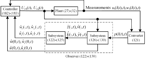
Refer to caption
Figure 4: Diagram of the output-feedback closed-loop system.
Theorem 4.

Considering the closed-loop system consisting of the plant (27)-(32), the observer (151)-(159) and the output-feedback controller (213)-(214), for initial values (w(x,0),wt(x,0))H2(0,L)×H1(0,L)𝑤𝑥0subscript𝑤𝑡𝑥0superscript𝐻20𝐿superscript𝐻10𝐿(w(x,0),w_{t}(x,0))\in H^{2}(0,L)\times H^{1}(0,L), (u(x,0),ut(x,0))H2(0,L)×H1(0,L)𝑢𝑥0subscript𝑢𝑡𝑥0superscript𝐻20𝐿superscript𝐻10𝐿(u(x,0),u_{t}(x,0))\in H^{2}(0,L)\times H^{1}(0,L), one obtains

1) there exist positive constants Υ5subscriptΥ5\Upsilon_{5} and σ5subscript𝜎5\sigma_{5} such that

(Ξ(t)+Ξ^(t))1/2Υ5(Ξ(0)+Ξ^(0))1/2eσ5t,superscriptΞ𝑡^Ξ𝑡12subscriptΥ5superscriptΞ0^Ξ012superscript𝑒subscript𝜎5𝑡\displaystyle\left(\Xi(t)+\hat{\Xi}(t)\right)^{1/2}\leq\Upsilon_{5}\left(\Xi(0)+\hat{\Xi}(0)\right)^{1/2}e^{-\sigma_{5}t}, (215)

where Ξ(t)Ξ𝑡\Xi(t) is given in (135) and Ξ^(t)^Ξ𝑡\hat{\Xi}(t) is defined as

Ξ^(t)=u^x(,t)2+u^t(,t)2+|u^(0,t)|2+|u^t(0,t)|2^Ξ𝑡superscriptnormsubscript^𝑢𝑥𝑡2superscriptnormsubscript^𝑢𝑡𝑡2superscript^𝑢0𝑡2superscriptsubscript^𝑢𝑡0𝑡2\displaystyle\hat{\Xi}(t)=\|\hat{u}_{x}(\cdot,t)\|^{2}+\|\hat{u}_{t}(\cdot,t)\|^{2}+\left|\hat{u}(0,t)\right|^{2}+\left|\hat{u}_{t}(0,t)\right|^{2}
+w^x(,t)2+w^t(,t)2+|w^(0,t)|2+|w^t(0,t)|2.superscriptnormsubscript^𝑤𝑥𝑡2superscriptnormsubscript^𝑤𝑡𝑡2superscript^𝑤0𝑡2superscriptsubscript^𝑤𝑡0𝑡2\displaystyle+\|\hat{w}_{x}(\cdot,t)\|^{2}+\|\hat{w}_{t}(\cdot,t)\|^{2}+\left|\hat{w}(0,t)\right|^{2}+\left|\hat{w}_{t}(0,t)\right|^{2}.

2) the output-feedback controllers (213)-(214) are bounded and exponentially convergent to zero.

Proof.

The output-feedback controller (213)-(214) can be written as

[Uo1(t),Uo2(t)]T=superscriptsubscript𝑈𝑜1𝑡subscript𝑈𝑜2𝑡𝑇absent\displaystyle[U_{o1}(t),U_{o2}(t)]^{T}= [Usf1(t),Usf2(t)]T+δ~(t)superscriptsubscript𝑈𝑠𝑓1𝑡subscript𝑈𝑠𝑓2𝑡𝑇~𝛿𝑡\displaystyle[U_{sf1}(t),U_{sf2}(t)]^{T}+\tilde{\delta}(t) (216)

considering (160)-(164), where Usf1(t),Usf2(t)subscript𝑈𝑠𝑓1𝑡subscript𝑈𝑠𝑓2𝑡U_{sf1}(t),U_{sf2}(t) are the state-feedback form presented as (115)-(116), and δ~(t)R2×1~𝛿𝑡superscript𝑅21\tilde{\delta}(t)\in R^{2\times 1} is

δ~(t)=~𝛿𝑡absent\displaystyle\tilde{\delta}(t)= 2R(l(t))1[0l(t)F(l(t),y)[u~t(y,t)d6(y)u~x(y,t),\displaystyle 2R(l(t))^{-1}\bigg{[}\int_{0}^{l(t)}F(l(t),y)[{\tilde{u}_{t}}(y,t)-\sqrt{{d_{6}}(y)}{\tilde{u}_{x}}(y,t),
w~t(y,t)d1(y)w~x(y,t)]Tdy\displaystyle{\tilde{w}_{t}}(y,t)-\sqrt{{d_{1}}(y)}{\tilde{w}_{x}}(y,t)]^{T}dy
+0l(t)N(l(t),y)[u~t(y,t)+d6(y)u~x(y,t),\displaystyle+\int_{0}^{l(t)}N(l(t),y)[{\tilde{u}_{t}}(y,t)+\sqrt{{d_{6}}(y)}{\tilde{u}_{x}}(y,t),
w~t(y,t)+d1(y)w~x(y,t)]dy\displaystyle{\tilde{w}_{t}}(y,t)+\sqrt{{d_{1}}(y)}{\tilde{w}_{x}}(y,t)]dy
+λ(l(t))[w~(0,t),w~t(0,t),u~(0,t),u~t(0,t)]T].\displaystyle+\lambda(l(t))[\tilde{w}(0,t),\tilde{w}_{t}(0,t),\tilde{u}(0,t),\tilde{u}_{t}(0,t)]^{T}\bigg{]}. (217)

Applying the output-feedback controller (216) into the plant (27)-(32), i.e., U1(t)=U1o(t),U2(t)=U2o(t)formulae-sequencesubscript𝑈1𝑡subscript𝑈1𝑜𝑡subscript𝑈2𝑡subscript𝑈2𝑜𝑡U_{1}(t)=U_{1o}(t),~{}U_{2}(t)=U_{2o}(t), recalling Theorem 1 and Theorem 3, together with (160)-(164), we achieve (215), i.e, property 1) in Theorem 4. Moreover, applying Theorem 2 which shows the state-feedback controllers [Usf1(t),Usf2(t)]Tsuperscriptsubscript𝑈𝑠𝑓1𝑡subscript𝑈𝑠𝑓2𝑡𝑇[U_{sf1}(t),U_{sf2}(t)]^{T} are exponentially convergent to zero and Theorem 3 which guarantees the exponential convergence to zero of δ~(t)~𝛿𝑡\tilde{\delta}(t) (217), boundedness and exponential convergence of the output feedback control input are obtained according to (216), i.e., the property 2) of Theorem 4. Therefore, the proof of Theorem 4 is completed. ∎

VI Simulation test on vibration suppression of DCV

The simulation is conducted based on the linear model (19)-(24) and actual nonlinear model (11)-(16) with unmodeled disturbances, respectively, where the first one is to verify the above theoretical results and the second one is to illustrate the effectiveness in the application of vibration control of DCV. Note that the time-varying domain plant with pre-determined time-varying functions l(t)𝑙𝑡l(t) and l˙(t)˙𝑙𝑡\dot{l}(t) shown in Fig. 5, is converted to the one on the fixed domain ι=[0,1]𝜄01\iota=[0,1] with time-varying coefficients related to l(t),l˙(t),l¨(t)𝑙𝑡˙𝑙𝑡¨𝑙𝑡l(t),\dot{l}(t),\ddot{l}(t) via introducing

ι=xl(t),𝜄𝑥𝑙𝑡\displaystyle\iota=\frac{x}{l(t)}, (218)

i.e., representing u(x,t)𝑢𝑥𝑡u(x,t) by u(ι,t)𝑢𝜄𝑡u(\iota,t) as

ux(x,t)subscript𝑢𝑥𝑥𝑡\displaystyle u_{x}(x,t) =1l(t)uι(ι,t),uxx(x,t)=1l(t)2uιι(ι,t),formulae-sequenceabsent1𝑙𝑡subscript𝑢𝜄𝜄𝑡subscript𝑢𝑥𝑥𝑥𝑡1𝑙superscript𝑡2subscript𝑢𝜄𝜄𝜄𝑡\displaystyle=\frac{1}{l(t)}{u_{\iota}(\iota,t)},~{}u_{xx}(x,t)=\frac{1}{l(t)^{2}}{u_{\iota\iota}(\iota,t)}, (219)
ut(x,t)subscript𝑢𝑡𝑥𝑡\displaystyle u_{t}(x,t) =ut(ι,t)l˙(t)ιl(t)uι(ι,t),absentsubscript𝑢𝑡𝜄𝑡˙𝑙𝑡𝜄𝑙𝑡subscript𝑢𝜄𝜄𝑡\displaystyle=u_{t}(\iota,t)-\frac{\dot{l}(t)\iota}{l(t)}{u_{\iota}(\iota,t)}, (220)
utt(x,t)subscript𝑢𝑡𝑡𝑥𝑡\displaystyle u_{tt}(x,t) =utt(ι,t)2l˙(t)ιl(t)uιt(ι,t)l˙(t)2ι2l(t)2uιι(ι,t)absentsubscript𝑢𝑡𝑡𝜄𝑡2˙𝑙𝑡𝜄𝑙𝑡subscript𝑢𝜄𝑡𝜄𝑡˙𝑙superscript𝑡2superscript𝜄2𝑙superscript𝑡2subscript𝑢𝜄𝜄𝜄𝑡\displaystyle={u_{tt}(\iota,t)}-\frac{2\dot{l}(t)\iota}{l(t)}{u_{\iota t}(\iota,t)}-\frac{\dot{l}(t)^{2}\iota^{2}}{l(t)^{2}}{u_{\iota\iota}(\iota,t)}
(l(t)l¨(t)2l¨(t)2)ιl(t)2uι(ι,t),𝑙𝑡¨𝑙𝑡2¨𝑙superscript𝑡2𝜄𝑙superscript𝑡2subscript𝑢𝜄𝜄𝑡\displaystyle\quad-\frac{(l(t)\ddot{l}(t)-2\ddot{l}(t)^{2})\iota}{l(t)^{2}}{u_{\iota}(\iota,t)}, (221)

and then the simulation is conducted based on the finite difference method with time step and space step as 0.001 and 0.05 respectively. The observer (151)-(159) is solved in the same way, and the following equations are used to obtain u^,w^^𝑢^𝑤\hat{u},\hat{w} from k^,y^,z^,v^^𝑘^𝑦^𝑧^𝑣\hat{k},\hat{y},\hat{z},\hat{v}

u^(ι,t)=0ι12d6(ι¯)(k^(ι¯,t)y^(ι¯,t))𝑑ι¯+C¯1W^(t),^𝑢𝜄𝑡superscriptsubscript0𝜄12subscript𝑑6¯𝜄^𝑘¯𝜄𝑡^𝑦¯𝜄𝑡differential-d¯𝜄subscript¯𝐶1^𝑊𝑡\displaystyle\hat{u}(\iota,t)=\int_{0}^{\iota}\frac{1}{2\sqrt{d_{6}(\bar{\iota})}}(\hat{k}(\bar{\iota},t)-\hat{y}(\bar{\iota},t))d{\bar{\iota}}+\bar{C}_{1}\hat{W}(t),
w^(ι,t)=0ι12d1(ι¯)(z^(ι¯,t)v^(ι¯,t))𝑑ι¯+C¯2W^(t)^𝑤𝜄𝑡superscriptsubscript0𝜄12subscript𝑑1¯𝜄^𝑧¯𝜄𝑡^𝑣¯𝜄𝑡differential-d¯𝜄subscript¯𝐶2^𝑊𝑡\displaystyle\hat{w}(\iota,t)=\int_{0}^{\iota}\frac{1}{2\sqrt{d_{1}(\bar{\iota})}}(\hat{z}(\bar{\iota},t)-\hat{v}(\bar{\iota},t))d{\bar{\iota}}+\bar{C}_{2}\hat{W}(t)

according to (151)-(154) and (164), where C¯1=[0,0,1,0]subscript¯𝐶10010\bar{C}_{1}=[0,0,1,0] and C¯2=[1,0,0,0]subscript¯𝐶21000\bar{C}_{2}=[1,0,0,0].

The initial conditions are defined according to the steady state, as ux(,0)=ε¯()subscript𝑢𝑥0¯𝜀u_{x}(\cdot,0)=\bar{\varepsilon}(\cdot), ut(,0)=0subscript𝑢𝑡00u_{t}(\cdot,0)=0 and wx(,0)=ϕ¯()subscript𝑤𝑥0¯italic-ϕw_{x}(\cdot,0)=-\bar{\phi}(\cdot), wt(,0)=0subscript𝑤𝑡00w_{t}(\cdot,0)=0. With defining u(0,0)=0𝑢000u(0,0)=0 and w(l(0),0)=0𝑤𝑙000w(l(0),0)=0, the initial conditions of (19)-(24) can thus be defined completely in the numerical calculation adopting the finite difference method. All initial conditions k^(,0),y^(,0),z^(,0),v^(,0),W^(0)^𝑘0^𝑦0^𝑧0^𝑣0^𝑊0\hat{k}(\cdot,0),\hat{y}(\cdot,0),\hat{z}(\cdot,0),\hat{v}(\cdot,0),\hat{W}(0) of the observer (151)-(159) are set as zero.

VI-A Linear model

VI-A1 System coefficients

Matching (27)-(32) with (19)-(24), we have the specific expressions of the coefficients in (27)-(32) as

d1(x)=32EAaϕ¯(x)2+T(x)mc,subscript𝑑1𝑥32𝐸subscript𝐴𝑎¯italic-ϕsuperscript𝑥2𝑇𝑥subscript𝑚𝑐\displaystyle d_{1}(x)=\frac{\frac{3}{2}EA_{a}\bar{\phi}(x)^{2}+T(x)}{m_{c}}, (222)
d2(x)=EAaε¯(x)+ρgmc,d3=EAaϕ¯(x)mc,formulae-sequencesubscript𝑑2𝑥𝐸subscript𝐴𝑎superscript¯𝜀𝑥𝜌𝑔subscript𝑚𝑐subscript𝑑3𝐸subscript𝐴𝑎superscript¯italic-ϕ𝑥subscript𝑚𝑐\displaystyle d_{2}(x)=\frac{EA_{a}\bar{\varepsilon}^{\prime}(x)+\rho g}{m_{c}},~{}d_{3}=\frac{-EA_{a}\bar{\phi}^{\prime}(x)}{m_{c}}, (223)
d4=cvmc,d5=0,d6=EAamc,d7(x)=EAaϕ¯(x)mc,formulae-sequencesubscript𝑑4subscript𝑐𝑣subscript𝑚𝑐formulae-sequencesubscript𝑑50formulae-sequencesubscript𝑑6𝐸subscript𝐴𝑎subscript𝑚𝑐subscript𝑑7𝑥𝐸subscript𝐴𝑎superscript¯italic-ϕ𝑥subscript𝑚𝑐\displaystyle d_{4}=\frac{-c_{v}}{m_{c}},~{}d_{5}=0,~{}d_{6}=\frac{EA_{a}}{m_{c}},~{}d_{7}(x)=\frac{-EA_{a}\bar{\phi}^{\prime}(x)}{m_{c}}, (224)
d8=d9=0,d10=cumc,d11=cwML,d12=EAaϕ¯(0)22ML,formulae-sequencesubscript𝑑8subscript𝑑90formulae-sequencesubscript𝑑10subscript𝑐𝑢subscript𝑚𝑐formulae-sequencesubscript𝑑11subscript𝑐𝑤subscript𝑀𝐿subscript𝑑12𝐸subscript𝐴𝑎¯italic-ϕsuperscript022subscript𝑀𝐿\displaystyle d_{8}=d_{9}=0,~{}d_{10}=\frac{-c_{u}}{m_{c}},~{}d_{11}=\frac{-c_{w}}{M_{L}},~{}d_{12}=\frac{-EA_{a}\bar{\phi}(0)^{2}}{2M_{L}}, (225)
d13=0,d14=EAaϕ¯(0)ML,d15=chML,d16=EAaML,formulae-sequencesubscript𝑑130formulae-sequencesubscript𝑑14𝐸subscript𝐴𝑎¯italic-ϕ0subscript𝑀𝐿formulae-sequencesubscript𝑑15subscript𝑐subscript𝑀𝐿subscript𝑑16𝐸subscript𝐴𝑎subscript𝑀𝐿\displaystyle d_{13}=0,~{}d_{14}=\frac{-EA_{a}\bar{\phi}(0)}{M_{L}},~{}d_{15}=\frac{-c_{h}}{M_{L}},d_{16}=\frac{-EA_{a}}{M_{L}}, (226)
d17=0,d18=EAaϕ¯(0)2ML,d19=1EAa,formulae-sequencesubscript𝑑170formulae-sequencesubscript𝑑18𝐸subscript𝐴𝑎¯italic-ϕ02subscript𝑀𝐿subscript𝑑191𝐸subscript𝐴𝑎\displaystyle d_{17}=0,~{}d_{18}=\frac{EA_{a}\bar{\phi}(0)}{2M_{L}},~{}d_{19}=\frac{1}{EA_{a}}, (227)
d20(l(t))=1EAaε¯(l(t))+EAa2ϕ¯(l(t))2+T(l(t)),subscript𝑑20𝑙𝑡1𝐸subscript𝐴𝑎¯𝜀𝑙𝑡𝐸subscript𝐴𝑎2¯italic-ϕsuperscript𝑙𝑡2𝑇𝑙𝑡\displaystyle d_{20}(l(t))=\frac{1}{EA_{a}\bar{\varepsilon}(l(t))+\frac{EA_{a}}{2}\bar{\phi}(l(t))^{2}+T(l(t))}, (228)

where T(x)𝑇𝑥T(x), ε¯(x)¯𝜀𝑥\bar{\varepsilon}(x) and ϕ¯(x)¯italic-ϕ𝑥\bar{\phi}(x) are given in (6), (17)-(18), and the values of the physical parameters are shown in Table III. x𝑥x in (222)-(228) can be represented by ι𝜄\iota via (218).

Refer to caption
Figure 5: Descending trajectory and velocity, i.e., the time-varying cable length l(t)𝑙𝑡l(t) and the changing rate l˙(t)˙𝑙𝑡\dot{l}(t).

VI-A2 Controller parameters

Apply the proposed controllers (213)-(214) into (19)-(24), where the approximate solution of the kernel equations (98)-(104) is also solved by the finite difference method on a fixed triangular domain 𝒟0={0yxL}subscript𝒟00𝑦𝑥𝐿{\mathcal{D}_{0}}=\{0\leq y\leq x\leq L\}, and then extract F(l(t),y),N(l(t),y)𝐹𝑙𝑡𝑦𝑁𝑙𝑡𝑦F(l(t),y),N(l(t),y) which would be used in the controller. The control parameters κ𝜅\kappa are chosen as

[κ11κ12κ13κ14κ21κ22κ23κ24]=[0.81.24.562.531.52]×103delimited-[]subscript𝜅11subscript𝜅12subscript𝜅13subscript𝜅14missing-subexpressionmissing-subexpressionmissing-subexpressionmissing-subexpressionmissing-subexpressionmissing-subexpressionmissing-subexpressionmissing-subexpressionmissing-subexpressionmissing-subexpressionmissing-subexpressionmissing-subexpressionmissing-subexpressionmissing-subexpressionmissing-subexpressionmissing-subexpressionsubscript𝜅21subscript𝜅22subscript𝜅23subscript𝜅24missing-subexpressionmissing-subexpressionmissing-subexpressionmissing-subexpressionmissing-subexpressionmissing-subexpressionmissing-subexpressionmissing-subexpressionmissing-subexpressionmissing-subexpressionmissing-subexpressionmissing-subexpressionmissing-subexpressionmissing-subexpressionmissing-subexpressionmissing-subexpressiondelimited-[]0.81.24.56missing-subexpressionmissing-subexpressionmissing-subexpressionmissing-subexpressionmissing-subexpressionmissing-subexpressionmissing-subexpressionmissing-subexpressionmissing-subexpressionmissing-subexpressionmissing-subexpressionmissing-subexpressionmissing-subexpressionmissing-subexpressionmissing-subexpressionmissing-subexpression2.531.52missing-subexpressionmissing-subexpressionmissing-subexpressionmissing-subexpressionmissing-subexpressionmissing-subexpressionmissing-subexpressionmissing-subexpressionmissing-subexpressionmissing-subexpressionmissing-subexpressionmissing-subexpressionmissing-subexpressionmissing-subexpressionmissing-subexpressionmissing-subexpressionsuperscript103\displaystyle\left[{\begin{array}[]{*{20}{c}}{{\kappa_{11}}}&{{\kappa_{12}}}&{{\kappa_{13}}}&{{\kappa_{14}}}\\ {{\kappa_{21}}}&{{\kappa_{22}}}&{{\kappa_{23}}}&{{\kappa_{24}}}\end{array}}\right]=\left[{\begin{array}[]{*{20}{c}}{0.8}&1.2&4.5&6\\ 2.5&3&1.5&2\end{array}}\right]\times 10^{3} (233)

which determines the kernel λ(x)𝜆𝑥\lambda(x) used in the controllers. A same process is used to obtain φ¯(x,l(t)),ψ¯(x,l(t))¯𝜑𝑥𝑙𝑡¯𝜓𝑥𝑙𝑡\bar{\varphi}(x,l(t)),\bar{\psi}(x,l(t)) used in the observer gains (196)-(197) and all elements in L0subscript𝐿0L_{0} are defined as 1.

Refer to caption
Figure 6: Responses of lateral vibrations w(x,t)𝑤𝑥𝑡w(x,t) without control.

VI-A3 Simulation results

Refer to caption
Figure 7: Responses of longitudinal vibrations u(x,t)𝑢𝑥𝑡u(x,t) without control.
Refer to caption
Figure 8: Closed-loop responses of longitudinal vibrations u(x,t)𝑢𝑥𝑡u(x,t).
Refer to caption
Figure 9: Closed-loop responses of lateral vibrations w(x,t)𝑤𝑥𝑡w(x,t).
Refer to caption
Figure 10: Control forces U1(t)subscript𝑈1𝑡U_{1}(t) and U2(t)subscript𝑈2𝑡U_{2}(t).
Refer to caption
Figure 11: Observer error of lateral vibrations w~(x,t)~𝑤𝑥𝑡\tilde{w}(x,t).
Refer to caption
Figure 12: Observer error of longitudinal vibrations u~(x,t)~𝑢𝑥𝑡\tilde{u}(x,t).

It can be seen from Fig. 6 that the large lateral vibrations whose oscillation range is up to 101010 m, persist in the whole operation time 120120120s in the case of without control. Even though the longitudinal vibrations in Fig. 7 are decaying because of the material damping coefficient cusubscript𝑐𝑢c_{u} of cable in Tab. III, the longitudinal vibration at the top of the cable (ι=1𝜄1\iota=1 in Fig. 6) is excessive and reduced slowly because this point bears the whole mass of the cable and payload resulting in large elastic deflections. Applying the proposed output-feedback two-directional vibration control forces at the ship-mounted crane, it is shown in Fig. 8 that the longitudinal vibrations are suppressed very fast, and the lateral vibrations also decay with a satisfied decay rate according to Fig. 9. The output-feedback control forces at the ship-mounted crane are shown in Fig. 10, where the states of the proposed observer are used. The performance of the observer on tracking the actual states can be seen in Figs. 11-12, which show the observer errors of both lateral and longitudinal vibrations are convergent to zero.

VI-B Actual nonlinear model with ocean current disturbances

The nonlinear model (11)-(16) in the simulation is generated via replacing ε¯(),ϕ¯()¯𝜀¯italic-ϕ\bar{\varepsilon}(\cdot),\bar{\phi}(\cdot) by ux(,t)subscript𝑢𝑥𝑡u_{x}(\cdot,t) and wx(,t)subscript𝑤𝑥𝑡-w_{x}(\cdot,t) in the linear model (19)-(24) respectively. Note that the time step and space step are changed to 0.00050.00050.0005 and 0.10.10.1 respectively in the finite difference method to ensure the existence of the numerical solution.

In practice, ocean current disturbances would act as external lateral oscillating drag forces f(ι,t)𝑓𝜄𝑡f(\iota,t) on the cable. In the simulation, f(ι,t)𝑓𝜄𝑡f(\iota,t) which is added in (12) and (14) converted to a fixed domain as above are defined as follows. Consider the time-varying ocean surface current velocity P(t)𝑃𝑡P(t) modeled by a first-order Gauss-Markov process [15]:

P˙(t)+μP(t)=𝒢(t),PminP(t)Pmax,formulae-sequence˙𝑃𝑡𝜇𝑃𝑡𝒢𝑡subscript𝑃𝑃𝑡subscript𝑃\displaystyle\dot{P}(t)+\mu P(t)=\mathcal{G}(t),~{}~{}P_{\min}\leq P(t)\leq P_{\max}, (234)

where 𝒢(t)𝒢𝑡\mathcal{G}(t) is Gaussian white noise. Constants Pmin,Pmaxsubscript𝑃subscript𝑃P_{\min},P_{\max} and μ𝜇\mu are chosen as 1.6ms11.6𝑚superscript𝑠11.6ms^{-1}, 2.4ms12.4𝑚superscript𝑠12.4ms^{-1} and 0 [16]. f(ι,t)𝑓𝜄𝑡f(\iota,t) can then be given as [16]:

f(ι,t)=𝑓𝜄𝑡absent\displaystyle f(\iota,t)= (0.9ι+0.1)12ρsCdP(t)2RDAD0.9𝜄0.112subscript𝜌𝑠subscript𝐶𝑑𝑃superscript𝑡2subscript𝑅𝐷subscript𝐴𝐷\displaystyle\left(0.9\iota+0.1\right)\frac{1}{2}\rho_{s}C_{d}P(t)^{2}R_{D}A_{D}
×cos(4πStP(t)RDt+ς)absent4𝜋subscript𝑆𝑡𝑃𝑡subscript𝑅𝐷𝑡𝜍\displaystyle\times\cos\left(4\pi\frac{S_{t}P(t)}{R_{D}}t+\varsigma\right) (235)

where 0.9ι+0.10.9𝜄0.10.9\iota+0.1 means the full disturbance load is applied at the top of the cable, i.e., the ocean surface, and linearly declines to its 0.10.10.1 at the bottom of the cable, i.e., the payload. Cd=1subscript𝐶𝑑1C_{d}=1 denotes the drag coefficient and ς=π𝜍𝜋\varsigma=\pi is the phase angle. AD=400subscript𝐴𝐷400A_{D}=400 denotes the amplitude of the oscillating drag force, St=0.2subscript𝑆𝑡0.2S_{t}=0.2 being the Strouhal number [14]. The ocean disturbances f𝑓f used in the simulation are shown in Fig. 13.
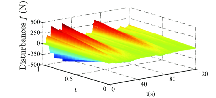
Refer to caption
Figure 13: Lateral oscillations drug forces from ocean current disturbances.
Refer to caption
Figure 14: Closed-loop responses of longitudinal vibrations u(x,t)𝑢𝑥𝑡u(x,t) in the actual nonlinear model with unmodeled disturbances.
Refer to caption
Figure 15: Closed-loop responses of lateral vibrations w(x,t)𝑤𝑥𝑡w(x,t) in the actual nonlinear model with unmodeled disturbances.
Refer to caption
Figure 16: Observer errors u~(,t)+w~(,t)~𝑢𝑡~𝑤𝑡\tilde{u}(\cdot,t)+\tilde{w}(\cdot,t) in the actual nonlinear model with unmodeled disturbances.
Refer to caption
Figure 17: Control forces in the actual nonlinear model.

The control parameters κ11subscript𝜅11\kappa_{11}, κ12subscript𝜅12\kappa_{12}, κ13subscript𝜅13\kappa_{13}, κ14subscript𝜅14\kappa_{14} and κ21subscript𝜅21\kappa_{21}, κ22subscript𝜅22\kappa_{22}, κ23subscript𝜅23\kappa_{23}, κ24subscript𝜅24\kappa_{24} are increased to twice and ten times of those in (233) respectively, considering the robust to the unmodeled disturbances. The observer parameters are kept same with those in Section VI-A. Apply the proposed output-feedback controller into the actual nonlinear model with the ocean current disturbances, it is shown in Figs. 14-15 that the longitudinal vibrations and lateral vibrations are reduced as time goes on. From Fig. 16, we know that the observer errors are convergent to a small range around zero. Simulation results in Section VI-B illustrate the effectiveness of the proposed control design applied into vibration suppression of DCV, where the output-feedback control inputs in this actual model are shown in Fig. 17.

VII Conclusion and future work

This work is motivated by a practical application of longitudinal-lateral vibration suppression for a deep-sea construction vessel which is used to install oil drilling equipment at the designated locations on the seafloor. The vibration dynamics of the DCV is derived by extended Hamilton’s principle resulting in a nonlinear wave PDE model, which is then linearized around the steady state to generate a linear model used in control design. The obtained specific model of the DCV is represented as a more general coupled wave PDE plant. Through Riemann transformations, the plant is converted to a 4×4444\times 4 coupled heterodirectional hyperbolic PDE-ODE system characterized by spatially-varying coefficients and on a time-varying domain, based on which the controller and observer designs are conducted via the backstepping method. The exponential stability results of the observer error system and the output-feedback closed-loop system, boundedness and exponential convergence of the control inputs are proved by Lyapunov analysis. The simulation test is conducted based on the both approximated linear model and actual nonlinear model to support the obtained theoretical results and verify that the proposed ship-mounted crane control forces can effectively suppress the undesired longitudinal-lateral vibrations in DCV.

The control design is on the basis of a completely known model, but some uncertainties, such as unknown model parameters, may appear in practice. In future work, the model uncertainties will be considered and some adaptive control technologies should be incorporated into the control design.

Appendix

Proof of Lemma 1: The boundary conditions in (98)-(104) are along the lines y=x𝑦𝑥y=x and y=0𝑦0y=0 and there are not conditions at the boundary x=l(t)𝑥𝑙𝑡x=l(t) on the triangular domain 𝒟𝒟{\mathcal{D}}. Therefore, we can extend the boundary x=l(t)𝑥𝑙𝑡x=l(t) in 𝒟𝒟\mathcal{D} to x=L𝑥𝐿x=L considering 0<l(t)L0𝑙𝑡𝐿0<l(t)\leq L in Assumption 3, to solve F,N𝐹𝑁F,N on a fixed triangular domain 𝒟0={0<y<x<L}subscript𝒟00𝑦𝑥𝐿{\mathcal{D}_{0}}=\{0<y<x<L\} and λ𝜆\lambda on a constant interval 0xL0𝑥𝐿0\leq x\leq L in (98)-(104). Note that the lines y=x𝑦𝑥y=x and y=0𝑦0y=0 are overlapped boundaries of the triangular domains 𝒟0subscript𝒟0{\mathcal{D}_{0}} and 𝒟𝒟{\mathcal{D}}, and 𝒟𝒟0𝒟subscript𝒟0{\mathcal{D}}\subseteq\mathcal{D}_{0}. Once the solutions of (98)-(104) on 𝒟0subscript𝒟0\mathcal{D}_{0} are obtained, the ones on the subset 𝒟𝒟\mathcal{D} are the required kernels F,N𝐹𝑁F,N and λ𝜆\lambda. To ensure the well-posedness of the kernel equations (98)-(104) on 𝒟0subscript𝒟0\mathcal{D}_{0}, we adding an additional artificial condition at x=L𝑥𝐿x=L for N21subscript𝑁21N_{21} as done in [17]. In the following, we will prove that there exists a unique solution of (98)-(104) on 𝒟0subscript𝒟0{\mathcal{D}_{0}} by showing it is in the form of a class of well-posed equations in [23], which ensures there exist a unique solution F,NL(𝒟)𝐹𝑁superscript𝐿𝒟F,N\in L^{\infty}(\mathcal{D}), λL([0,l(t)])𝜆superscript𝐿0𝑙𝑡\lambda\in L^{\infty}([0,l(t)]).

Expanding (98)-(104) on 𝒟0subscript𝒟0\mathcal{D}_{0}, we know Fij(x,y)1i,j2subscript𝐹𝑖𝑗subscript𝑥𝑦formulae-sequence1𝑖𝑗2F_{ij}(x,y)_{1\leq i,j\leq 2}, Nij(x,y)1i,j2subscript𝑁𝑖𝑗subscript𝑥𝑦formulae-sequence1𝑖𝑗2N_{ij}(x,y)_{1\leq i,j\leq 2} should satisfy following coupled hyperbolic PDEs:

d6(x)F11x(x,y)d6(y)F11y(x,y)subscript𝑑6𝑥subscript𝐹11𝑥𝑥𝑦subscript𝑑6𝑦subscript𝐹11𝑦𝑥𝑦\displaystyle\sqrt{{d_{6}}(x)}{F_{11x}}(x,y)-\sqrt{{d_{6}}(y)}{F_{11y}}(x,y)
=[d10(y)2s1(y)]N11(x,y)+[d5(y)2d3(y)2d6(y)]N12(x,y)absentdelimited-[]subscript𝑑10𝑦2subscript𝑠1𝑦subscript𝑁11𝑥𝑦delimited-[]subscript𝑑5𝑦2subscript𝑑3𝑦2subscript𝑑6𝑦subscript𝑁12𝑥𝑦\displaystyle=[\frac{{{d_{10}}(y)}}{2}-{s_{1}}(y)]{N_{11}}(x,y)+[\frac{{{d_{5}}(y)}}{2}-\frac{{{d_{3}}(y)}}{{2\sqrt{{d_{6}}(y)}}}]{N_{12}}(x,y)
+[d10(y)2s1(y)+d6(y)d10(x)2+s1(x)]F11(x,y)delimited-[]subscript𝑑10𝑦2subscript𝑠1𝑦superscriptsubscript𝑑6𝑦subscript𝑑10𝑥2subscript𝑠1𝑥subscript𝐹11𝑥𝑦\displaystyle+[\frac{{{d_{10}}(y)}}{2}-{s_{1}}(y)+{\sqrt{{d_{6}}(y)}^{\prime}}-\frac{{{d_{10}}(x)}}{2}+{s_{1}}(x)]{F_{11}}(x,y)
+[d5(y)2d3(y)2d6(y)]F12(x,y),delimited-[]subscript𝑑5𝑦2subscript𝑑3𝑦2subscript𝑑6𝑦subscript𝐹12𝑥𝑦\displaystyle+[\frac{{{d_{5}}(y)}}{2}-\frac{{{d_{3}}(y)}}{{2\sqrt{{d_{6}}(y)}}}]{F_{12}}(x,y), (236)
d6(x)F12x(x,y)d1(y)F12y(x,y)subscript𝑑6𝑥subscript𝐹12𝑥𝑥𝑦subscript𝑑1𝑦subscript𝐹12𝑦𝑥𝑦\displaystyle\sqrt{{d_{6}}(x)}{F_{12x}}(x,y)-\sqrt{{d_{1}}(y)}{F_{12y}}(x,y)
=[d9(y)2d7(y)2d1(y)]N11(x,y)+[d4(y)2s2(y)]N12(x,y)absentdelimited-[]subscript𝑑9𝑦2subscript𝑑7𝑦2subscript𝑑1𝑦subscript𝑁11𝑥𝑦delimited-[]subscript𝑑4𝑦2subscript𝑠2𝑦subscript𝑁12𝑥𝑦\displaystyle=[\frac{{{d_{9}}(y)}}{2}-\frac{{{d_{7}}(y)}}{{2\sqrt{{d_{1}}(y)}}}]{N_{11}}(x,y)+[\frac{{{d_{4}}(y)}}{2}-{s_{2}}(y)]{N_{12}}(x,y)
+[d4(y)2s2(y)+d1(y)d10(x)2+s1(x)]F12(x,y)delimited-[]subscript𝑑4𝑦2subscript𝑠2𝑦superscriptsubscript𝑑1𝑦subscript𝑑10𝑥2subscript𝑠1𝑥subscript𝐹12𝑥𝑦\displaystyle+[\frac{{{d_{4}}(y)}}{2}-{s_{2}}(y)+{\sqrt{{d_{1}}(y)}^{\prime}}-\frac{{{d_{10}}(x)}}{2}+{s_{1}}(x)]{F_{12}}(x,y)
+[d9(y)2d7(y)2d1(y)]F11(x,y),delimited-[]subscript𝑑9𝑦2subscript𝑑7𝑦2subscript𝑑1𝑦subscript𝐹11𝑥𝑦\displaystyle+[\frac{{{d_{9}}(y)}}{2}-\frac{{{d_{7}}(y)}}{{2\sqrt{{d_{1}}(y)}}}]{F_{11}}(x,y), (237)
d1(x)F21x(x,y)d6(y)F21y(x,y)subscript𝑑1𝑥subscript𝐹21𝑥𝑥𝑦subscript𝑑6𝑦subscript𝐹21𝑦𝑥𝑦\displaystyle\sqrt{{d_{1}}(x)}{F_{21x}}(x,y)-\sqrt{{d_{6}}(y)}{F_{21y}}(x,y)
=[d10(y)2s1(y)]N21(x,y)+[d5(y)2d3(y)2d6(y)]N22(x,y)absentdelimited-[]subscript𝑑10𝑦2subscript𝑠1𝑦subscript𝑁21𝑥𝑦delimited-[]subscript𝑑5𝑦2subscript𝑑3𝑦2subscript𝑑6𝑦subscript𝑁22𝑥𝑦\displaystyle=[\frac{{{d_{10}}(y)}}{2}-{s_{1}}(y)]{N_{21}}(x,y)+[\frac{{{d_{5}}(y)}}{2}-\frac{{{d_{3}}(y)}}{{2\sqrt{{d_{6}}(y)}}}]{N_{22}}(x,y)
+[d10(y)2s1(y)+d6(y)d4(x)2+s2(x)]F21(x,y)delimited-[]subscript𝑑10𝑦2subscript𝑠1𝑦superscriptsubscript𝑑6𝑦subscript𝑑4𝑥2subscript𝑠2𝑥subscript𝐹21𝑥𝑦\displaystyle+[\frac{{{d_{10}}(y)}}{2}-{s_{1}}(y)+{\sqrt{{d_{6}}(y)}^{\prime}}-\frac{{{d_{4}}(x)}}{2}+{s_{2}}(x)]{F_{21}}(x,y)
+[d5(y)2d3(y)2d6(y)]F22(x,y),delimited-[]subscript𝑑5𝑦2subscript𝑑3𝑦2subscript𝑑6𝑦subscript𝐹22𝑥𝑦\displaystyle+[\frac{{{d_{5}}(y)}}{2}-\frac{{{d_{3}}(y)}}{{2\sqrt{{d_{6}}(y)}}}]{F_{22}}(x,y), (238)
d1(x)F22x(x,y)d1(y)F22y(x,y)subscript𝑑1𝑥subscript𝐹22𝑥𝑥𝑦subscript𝑑1𝑦subscript𝐹22𝑦𝑥𝑦\displaystyle\sqrt{{d_{1}}(x)}{F_{22x}}(x,y)-\sqrt{{d_{1}}(y)}{F_{22y}}(x,y)
=[d9(y)2d7(y)2d1(y)]N21(x,y)+[d4(y)2s2(y)]N22(x,y)absentdelimited-[]subscript𝑑9𝑦2subscript𝑑7𝑦2subscript𝑑1𝑦subscript𝑁21𝑥𝑦delimited-[]subscript𝑑4𝑦2subscript𝑠2𝑦subscript𝑁22𝑥𝑦\displaystyle=[\frac{{{d_{9}}(y)}}{2}-\frac{{{d_{7}}(y)}}{{2\sqrt{{d_{1}}(y)}}}]{N_{21}}(x,y)+[\frac{{{d_{4}}(y)}}{2}-{s_{2}}(y)]{N_{22}}(x,y)
+[d4(y)2s2(y)+d1(y)d4(x)2+s2(x)]F22(x,y)delimited-[]subscript𝑑4𝑦2subscript𝑠2𝑦superscriptsubscript𝑑1𝑦subscript𝑑4𝑥2subscript𝑠2𝑥subscript𝐹22𝑥𝑦\displaystyle+[\frac{{{d_{4}}(y)}}{2}-{s_{2}}(y)+{\sqrt{{d_{1}}(y)}^{\prime}}-\frac{{{d_{4}}(x)}}{2}+{s_{2}}(x)]{F_{22}}(x,y)
+[d9(y)2d7(y)2d1(y)]F21(x,y),delimited-[]subscript𝑑9𝑦2subscript𝑑7𝑦2subscript𝑑1𝑦subscript𝐹21𝑥𝑦\displaystyle+[\frac{{{d_{9}}(y)}}{2}-\frac{{{d_{7}}(y)}}{{2\sqrt{{d_{1}}(y)}}}]{F_{21}}(x,y), (239)
d6(x)N11x(x,y)+d6(y)N11y(x,y)subscript𝑑6𝑥subscript𝑁11𝑥𝑥𝑦subscript𝑑6𝑦subscript𝑁11𝑦𝑥𝑦\displaystyle\sqrt{{d_{6}}(x)}{N_{11x}}(x,y)+\sqrt{{d_{6}}(y)}{N_{11y}}(x,y)
=[s1(y)+d10(y)2]F11(x,y)+[d3(y)2d6(y)+d5(y)2]F12(x,y)absentdelimited-[]subscript𝑠1𝑦subscript𝑑10𝑦2subscript𝐹11𝑥𝑦delimited-[]subscript𝑑3𝑦2subscript𝑑6𝑦subscript𝑑5𝑦2subscript𝐹12𝑥𝑦\displaystyle=[{s_{1}}(y)+\frac{{{d_{10}}(y)}}{2}]{F_{11}}(x,y)+[\frac{{{d_{3}}(y)}}{{2\sqrt{{d_{6}}(y)}}}+\frac{{{d_{5}}(y)}}{2}]{F_{12}}(x,y)
+[s1(y)+d10(y)2d6(y)s1(x)d10(x)2]N11(x,y)delimited-[]subscript𝑠1𝑦subscript𝑑10𝑦2superscriptsubscript𝑑6𝑦subscript𝑠1𝑥subscript𝑑10𝑥2subscript𝑁11𝑥𝑦\displaystyle+[{s_{1}}(y)+\frac{{{d_{10}}(y)}}{2}-{\sqrt{{d_{6}}(y)}^{\prime}}-{s_{1}}(x)-\frac{{{d_{10}}(x)}}{2}]{N_{11}}(x,y)
+[d3(y)2d6(y)+d5(y)2]N12(x,y),delimited-[]subscript𝑑3𝑦2subscript𝑑6𝑦subscript𝑑5𝑦2subscript𝑁12𝑥𝑦\displaystyle+[\frac{{{d_{3}}(y)}}{{2\sqrt{{d_{6}}(y)}}}+\frac{{{d_{5}}(y)}}{2}]{N_{12}}(x,y), (240)
d6(x)N12x(x,y)+d1(y)N12y(x,y)subscript𝑑6𝑥subscript𝑁12𝑥𝑥𝑦subscript𝑑1𝑦subscript𝑁12𝑦𝑥𝑦\displaystyle\sqrt{{d_{6}}(x)}{N_{12x}}(x,y)+\sqrt{{d_{1}}(y)}{N_{12y}}(x,y)
=[d7(y)2d1(y)+d9(y)2]F11(x,y)+[s2(y)+d4(y)2]F12(x,y)absentdelimited-[]subscript𝑑7𝑦2subscript𝑑1𝑦subscript𝑑9𝑦2subscript𝐹11𝑥𝑦delimited-[]subscript𝑠2𝑦subscript𝑑4𝑦2subscript𝐹12𝑥𝑦\displaystyle=[\frac{{{d_{7}}(y)}}{{2\sqrt{{d_{1}}(y)}}}+\frac{{{d_{9}}(y)}}{2}]{F_{11}}(x,y)+[{s_{2}}(y)+\frac{{{d_{4}}(y)}}{2}]{F_{12}}(x,y)
+[s2(y)+d4(y)2d1(y)s1(x)d10(x)2]N12(x,y)delimited-[]subscript𝑠2𝑦subscript𝑑4𝑦2superscriptsubscript𝑑1𝑦subscript𝑠1𝑥subscript𝑑10𝑥2subscript𝑁12𝑥𝑦\displaystyle+[{s_{2}}(y)+\frac{{{d_{4}}(y)}}{2}-{\sqrt{{d_{1}}(y)}^{\prime}}-{s_{1}}(x)-\frac{{{d_{10}}(x)}}{2}]{N_{12}}(x,y)
+[d7(y)2d1(y)+d9(y)2]N11(x,y),delimited-[]subscript𝑑7𝑦2subscript𝑑1𝑦subscript𝑑9𝑦2subscript𝑁11𝑥𝑦\displaystyle+[\frac{{{d_{7}}(y)}}{{2\sqrt{{d_{1}}(y)}}}+\frac{{{d_{9}}(y)}}{2}]{N_{11}}(x,y), (241)
d1(x)N21x(x,y)+d6(y)N21y(x,y)subscript𝑑1𝑥subscript𝑁21𝑥𝑥𝑦subscript𝑑6𝑦subscript𝑁21𝑦𝑥𝑦\displaystyle\sqrt{{d_{1}}(x)}{N_{21x}}(x,y)+\sqrt{{d_{6}}(y)}{N_{21y}}(x,y)
=[s1(y)+d10(y)2]F21(x,y)+[d3(y)2d6(y)+d5(y)2]F22(x,y)absentdelimited-[]subscript𝑠1𝑦subscript𝑑10𝑦2subscript𝐹21𝑥𝑦delimited-[]subscript𝑑3𝑦2subscript𝑑6𝑦subscript𝑑5𝑦2subscript𝐹22𝑥𝑦\displaystyle=[{s_{1}}(y)+\frac{{{d_{10}}(y)}}{2}]{F_{21}}(x,y)+[\frac{{{d_{3}}(y)}}{{2\sqrt{{d_{6}}(y)}}}+\frac{{{d_{5}}(y)}}{2}]{F_{22}}(x,y)
+[s1(y)+d10(y)2d6(y)s2(x)d4(x)2]N21(x,y)delimited-[]subscript𝑠1𝑦subscript𝑑10𝑦2superscriptsubscript𝑑6𝑦subscript𝑠2𝑥subscript𝑑4𝑥2subscript𝑁21𝑥𝑦\displaystyle+[{s_{1}}(y)+\frac{{{d_{10}}(y)}}{2}-{\sqrt{{d_{6}}(y)}^{\prime}}-{s_{2}}(x)-\frac{{{d_{4}}(x)}}{2}]{N_{21}}(x,y)
+[d3(y)2d6(y)+d5(y)2]N22(x,y),delimited-[]subscript𝑑3𝑦2subscript𝑑6𝑦subscript𝑑5𝑦2subscript𝑁22𝑥𝑦\displaystyle+[\frac{{{d_{3}}(y)}}{{2\sqrt{{d_{6}}(y)}}}+\frac{{{d_{5}}(y)}}{2}]{N_{22}}(x,y), (242)
d1(x)N22x(x,y)+d1(y)N22y(x,y)subscript𝑑1𝑥subscript𝑁22𝑥𝑥𝑦subscript𝑑1𝑦subscript𝑁22𝑦𝑥𝑦\displaystyle\sqrt{{d_{1}}(x)}{N_{22x}}(x,y)+\sqrt{{d_{1}}(y)}{N_{22y}}(x,y)
=[d7(y)2d1(y)+d9(y)2]F21(x,y)+[s2(y)+d4(y)2]F22(x,y)absentdelimited-[]subscript𝑑7𝑦2subscript𝑑1𝑦subscript𝑑9𝑦2subscript𝐹21𝑥𝑦delimited-[]subscript𝑠2𝑦subscript𝑑4𝑦2subscript𝐹22𝑥𝑦\displaystyle=[\frac{{{d_{7}}(y)}}{{2\sqrt{{d_{1}}(y)}}}+\frac{{{d_{9}}(y)}}{2}]{F_{21}}(x,y)+[{s_{2}}(y)+\frac{{{d_{4}}(y)}}{2}]{F_{22}}(x,y)
+[s2(y)+d4(y)2d1(y)s2(x)d4(x)2]N22(x,y)delimited-[]subscript𝑠2𝑦subscript𝑑4𝑦2superscriptsubscript𝑑1𝑦subscript𝑠2𝑥subscript𝑑4𝑥2subscript𝑁22𝑥𝑦\displaystyle+[{s_{2}}(y)+\frac{{{d_{4}}(y)}}{2}-{\sqrt{{d_{1}}(y)}^{\prime}}-{s_{2}}(x)-\frac{{{d_{4}}(x)}}{2}]{N_{22}}(x,y)
+[d7(y)2d1(x)+d9(y)2]N21(x,y)delimited-[]subscript𝑑7𝑦2subscript𝑑1𝑥subscript𝑑9𝑦2subscript𝑁21𝑥𝑦\displaystyle+[\frac{{{d_{7}}(y)}}{{2\sqrt{{d_{1}}(x)}}}+\frac{{{d_{9}}(y)}}{2}]{N_{21}}(x,y) (243)

along with the following set of boundary conditions:

F11(x,x)=d10(x)+2s1(x)4d6(x),subscript𝐹11𝑥𝑥subscript𝑑10𝑥2subscript𝑠1𝑥4subscript𝑑6𝑥\displaystyle{F_{11}}(x,x)=\frac{{-{d_{10}}(x)+2{s_{1}}(x)}}{{4\sqrt{{d_{6}}(x)}}}, (244)
F12(x,x)=d9(x)d1(x)+d7(x)2(d6(x)+d1(x))d1(x),subscript𝐹12𝑥𝑥subscript𝑑9𝑥subscript𝑑1𝑥subscript𝑑7𝑥2subscript𝑑6𝑥subscript𝑑1𝑥subscript𝑑1𝑥\displaystyle{F_{12}}(x,x)=\frac{{-{d_{9}}(x)}\sqrt{{d_{1}}(x)}+{d_{7}}(x)}{{2(\sqrt{{d_{6}}(x)}+\sqrt{{d_{1}}(x)})\sqrt{{d_{1}}(x)}}}, (245)
F21(x,x)=d5(x)d6(x)+d3(x)2(d6(x)+d1(x))d6(x),subscript𝐹21𝑥𝑥subscript𝑑5𝑥subscript𝑑6𝑥subscript𝑑3𝑥2subscript𝑑6𝑥subscript𝑑1𝑥subscript𝑑6𝑥\displaystyle{F_{21}}(x,x)=\frac{{-{d_{5}}(x)}\sqrt{{d_{6}}(x)}+{d_{3}}(x)}{{2(\sqrt{{d_{6}}(x)}+\sqrt{{d_{1}}(x)})\sqrt{{d_{6}}(x)}}}, (246)
F22(x,x)=d4(x)+2s2(x)4d1(x),subscript𝐹22𝑥𝑥subscript𝑑4𝑥2subscript𝑠2𝑥4subscript𝑑1𝑥\displaystyle{F_{22}}(x,x)=\frac{{-{d_{4}}(x)+2s_{2}(x)}}{{4\sqrt{{d_{1}}(x)}}}, (247)
N12(x,x)=d7(x)2d1(x)d9(x)2d6(x)d1(x),subscript𝑁12𝑥𝑥subscript𝑑7𝑥2subscript𝑑1𝑥subscript𝑑9𝑥2subscript𝑑6𝑥subscript𝑑1𝑥\displaystyle{N_{12}}(x,x){\rm{=}}\frac{{\frac{{-{d_{7}}(x)}}{{2\sqrt{{d_{1}}(x)}}}-\frac{{{d_{9}}(x)}}{2}}}{{\sqrt{{d_{6}}(x)}-\sqrt{{d_{1}}(x)}}}, (248)
N21(x,x)=d3(x)2d6(x)d5(x)2d1(x)d6(x),subscript𝑁21𝑥𝑥subscript𝑑3𝑥2subscript𝑑6𝑥subscript𝑑5𝑥2subscript𝑑1𝑥subscript𝑑6𝑥\displaystyle{N_{21}}(x,x){\rm{=}}\frac{{\frac{{-{d_{3}}(x)}}{{2\sqrt{{d_{6}}(x)}}}-\frac{{{d_{5}}(x)}}{2}}}{{\sqrt{{d_{1}}(x)}-\sqrt{{d_{6}}(x)}}}, (249)
N11(x,0)=F11(x,0)+d14λ12(x)d6(0)+d16λ14(x)d6(0),subscript𝑁11𝑥0subscript𝐹11𝑥0subscript𝑑14subscript𝜆12𝑥subscript𝑑60subscript𝑑16subscript𝜆14𝑥subscript𝑑60\displaystyle{N_{11}}(x,0)=-{F_{11}}(x,0)+\frac{{{d_{14}}{\lambda_{12}}(x)}}{{{d_{6}}(0)}}+\frac{{{d_{16}}{\lambda_{14}}(x)}}{{{d_{6}}(0)}}, (250)
N12(x,0)=F12(x,0)+d12λ12(x)d1(0)+d18λ14(x)d1(0),subscript𝑁12𝑥0subscript𝐹12𝑥0subscript𝑑12subscript𝜆12𝑥subscript𝑑10subscript𝑑18subscript𝜆14𝑥subscript𝑑10\displaystyle{N_{12}}(x,0)=-{F_{12}}(x,0)+\frac{{{d_{12}}{\lambda_{12}}(x)}}{{{d_{1}}(0)}}+\frac{{{d_{18}}{\lambda_{14}}(x)}}{{{d_{1}}(0)}}, (251)
N21(x,0)=F21(x,0)subscript𝑁21𝑥0subscript𝐹21𝑥0\displaystyle{N_{21}}(x,0)=-{F_{21}}(x,0)
+g0(x)d6(0)+d14λ22(x)+d16λ24(x)d6(0),subscript𝑔0𝑥subscript𝑑60subscript𝑑14subscript𝜆22𝑥subscript𝑑16subscript𝜆24𝑥subscript𝑑60\displaystyle\quad\quad\quad\quad+\frac{{g_{0}}(x)\sqrt{{d_{6}}(0)}+{{d_{14}}{\lambda_{22}}(x)}+{{{d_{16}}{\lambda_{24}}(x)}}}{{{d_{6}}(0)}}, (252)
N22(x,0)=F22(x,0)+d12λ22(x)d1(0)+d18λ24(x)d1(0),subscript𝑁22𝑥0subscript𝐹22𝑥0subscript𝑑12subscript𝜆22𝑥subscript𝑑10subscript𝑑18subscript𝜆24𝑥subscript𝑑10\displaystyle{N_{22}}(x,0)=-{F_{22}}(x,0)+\frac{{{d_{12}}{\lambda_{22}}(x)}}{{{d_{1}}(0)}}+\frac{{{d_{18}}{\lambda_{24}}(x)}}{{{d_{1}}(0)}}, (253)
N21(L,y)=0,subscript𝑁21𝐿𝑦0\displaystyle N_{21}(L,y)=0, (254)

where (254) is the artificial boundary condition. Besides, λij(x)1i2,1j4subscript𝜆𝑖𝑗subscript𝑥formulae-sequence1𝑖21𝑗4{\lambda_{ij}}(x)_{1\leq i\leq 2,1\leq j\leq 4} should satisfy the following ODEs:

d6(x)λ11(x)+[s1(x)+d10(x)2]λ11(x)=0,subscript𝑑6𝑥superscriptsubscript𝜆11𝑥delimited-[]subscript𝑠1𝑥subscript𝑑10𝑥2subscript𝜆11𝑥0\displaystyle\sqrt{{d_{6}}(x)}{\lambda_{11}}^{\prime}(x)+[{s_{1}}(x)+\frac{{{d_{10}}(x)}}{2}]{\lambda_{11}}(x)=0, (255)
d6(x)λ12(x)+[s1(x)+d10(x)2d11+d12d1(0)]λ12(x)subscript𝑑6𝑥superscriptsubscript𝜆12𝑥delimited-[]subscript𝑠1𝑥subscript𝑑10𝑥2subscript𝑑11subscript𝑑12subscript𝑑10subscript𝜆12𝑥\displaystyle\sqrt{{d_{6}}(x)}{\lambda_{12}}^{\prime}(x)+[{s_{1}}(x)+\frac{{{d_{10}}(x)}}{2}-{d_{11}}+\frac{{{d_{12}}}}{{\sqrt{{d_{1}}(0)}}}]{\lambda_{12}}(x)
λ11(x)(d17d18d1(0))λ14(x)subscript𝜆11𝑥subscript𝑑17subscript𝑑18subscript𝑑10subscript𝜆14𝑥\displaystyle-{\lambda_{11}}(x)-({d_{17}}-\frac{{{d_{18}}}}{{\sqrt{{d_{1}}(0)}}}){\lambda_{14}}(x)
2d1(0)F12(x,0)=0,2subscript𝑑10subscript𝐹12𝑥00\displaystyle-2\sqrt{{d_{1}}(0)}{F_{12}}(x,0)=0, (256)
d6(x)λ13(x)+[s1(x)+d10(x)2]λ13(x)=0,subscript𝑑6𝑥superscriptsubscript𝜆13𝑥delimited-[]subscript𝑠1𝑥subscript𝑑10𝑥2subscript𝜆13𝑥0\displaystyle\sqrt{{d_{6}}(x)}{\lambda_{13}}^{\prime}(x)+[{s_{1}}(x)+\frac{{{d_{10}}(x)}}{2}]{\lambda_{13}}(x)=0, (257)
d6(x)λ14(x)+[s1(x)+d10(x)2d15+d16d6(0)]λ14(x)subscript𝑑6𝑥superscriptsubscript𝜆14𝑥delimited-[]subscript𝑠1𝑥subscript𝑑10𝑥2subscript𝑑15subscript𝑑16subscript𝑑60subscript𝜆14𝑥\displaystyle\sqrt{{d_{6}}(x)}{\lambda_{14}}^{\prime}(x)+[{s_{1}}(x)+\frac{{{d_{10}}(x)}}{2}-{d_{15}}+\frac{{{d_{16}}}}{{\sqrt{{d_{6}}(0)}}}]{\lambda_{14}}(x)
λ13(x)(d13d14d6(0))λ12(x)subscript𝜆13𝑥subscript𝑑13subscript𝑑14subscript𝑑60subscript𝜆12𝑥\displaystyle-{\lambda_{13}}(x)-({d_{13}}-\frac{{{d_{14}}}}{{\sqrt{{d_{6}}(0)}}}){\lambda_{12}}(x)
2d6(0)F11(x,0)=0,2subscript𝑑60subscript𝐹11𝑥00\displaystyle-2\sqrt{{d_{6}}(0)}{F_{11}}(x,0)=0, (258)
d1(x)λ21(x)+[s2(x)+d4(x)2]λ21(x)+g0(x)λ11(0)=0,subscript𝑑1𝑥superscriptsubscript𝜆21𝑥delimited-[]subscript𝑠2𝑥subscript𝑑4𝑥2subscript𝜆21𝑥subscript𝑔0𝑥subscript𝜆1100\displaystyle\sqrt{{d_{1}}(x)}{\lambda_{21}}^{\prime}(x)+[{s_{2}}(x)+\frac{{{d_{4}}(x)}}{2}]{\lambda_{21}}(x)+{g_{0}}(x){\lambda_{11}}(0){\rm{=}}0, (259)
d1(x)λ22(x)+[s2(x)+d4(x)2d11+d12d1(0)]λ22(x)subscript𝑑1𝑥superscriptsubscript𝜆22𝑥delimited-[]subscript𝑠2𝑥subscript𝑑4𝑥2subscript𝑑11subscript𝑑12subscript𝑑10subscript𝜆22𝑥\displaystyle\sqrt{{d_{1}}(x)}{\lambda_{22}}^{\prime}(x)+[{s_{2}}(x)+\frac{{{d_{4}}(x)}}{2}-{d_{11}}+\frac{{{d_{12}}}}{{\sqrt{{d_{1}}(0)}}}]{\lambda_{22}}(x)
λ21(x)(d17d18d1(0))λ24(x)subscript𝜆21𝑥subscript𝑑17subscript𝑑18subscript𝑑10subscript𝜆24𝑥\displaystyle-{\lambda_{21}}(x)-({d_{17}}-\frac{{{d_{18}}}}{{\sqrt{{d_{1}}(0)}}}){\lambda_{24}}(x)
2d1(0)F22(x,0)+g0(x)λ12(0)=0,2subscript𝑑10subscript𝐹22𝑥0subscript𝑔0𝑥subscript𝜆1200\displaystyle-2\sqrt{{d_{1}}(0)}{F_{22}}(x,0)+{g_{0}}(x){\lambda_{12}}(0)=0, (260)
d1(x)λ23(x)+[s2(x)+d4(x)2]λ23(x)+g0(x)λ13(0)=0,subscript𝑑1𝑥superscriptsubscript𝜆23𝑥delimited-[]subscript𝑠2𝑥subscript𝑑4𝑥2subscript𝜆23𝑥subscript𝑔0𝑥subscript𝜆1300\displaystyle\sqrt{{d_{1}}(x)}{\lambda_{23}}^{\prime}(x)+[{s_{2}}(x)+\frac{{{d_{4}}(x)}}{2}]{\lambda_{23}}(x)+{g_{0}}(x){\lambda_{13}}(0)=0, (261)
d1(x)λ24(x)+[s2(x)+d4(x)2d15+d16d6(0)]λ24(x)subscript𝑑1𝑥superscriptsubscript𝜆24𝑥delimited-[]subscript𝑠2𝑥subscript𝑑4𝑥2subscript𝑑15subscript𝑑16subscript𝑑60subscript𝜆24𝑥\displaystyle\sqrt{{d_{1}}(x)}{\lambda_{24}}^{\prime}(x)+[{s_{2}}(x)+\frac{{{d_{4}}(x)}}{2}-{d_{15}}+\frac{{{d_{16}}}}{{\sqrt{{d_{6}}(0)}}}]{\lambda_{24}}(x)
(d13d14d6(0))λ22(x)λ23(x)subscript𝑑13subscript𝑑14subscript𝑑60subscript𝜆22𝑥subscript𝜆23𝑥\displaystyle-({d_{13}}-\frac{{{d_{14}}}}{{\sqrt{{d_{6}}(0)}}}){\lambda_{22}}(x)-{\lambda_{23}}(x)
2d6(0)F21(x,0)+g0(x)λ14(0)=0,2subscript𝑑60subscript𝐹21𝑥0subscript𝑔0𝑥subscript𝜆1400\displaystyle-2\sqrt{{d_{6}}(0)}{F_{21}}(x,0)+{g_{0}}(x){\lambda_{14}}(0)=0, (262)

with initial conditions:

[λ11(0)λ12(0)λ13(0)λ14(0)λ21(0)λ22(0)λ23(0)λ24(0)]delimited-[]subscript𝜆110subscript𝜆120subscript𝜆130subscript𝜆140missing-subexpressionmissing-subexpressionmissing-subexpressionmissing-subexpressionmissing-subexpressionmissing-subexpressionmissing-subexpressionmissing-subexpressionmissing-subexpressionmissing-subexpressionmissing-subexpressionmissing-subexpressionmissing-subexpressionmissing-subexpressionmissing-subexpressionmissing-subexpressionsubscript𝜆210subscript𝜆220subscript𝜆230subscript𝜆240missing-subexpressionmissing-subexpressionmissing-subexpressionmissing-subexpressionmissing-subexpressionmissing-subexpressionmissing-subexpressionmissing-subexpressionmissing-subexpressionmissing-subexpressionmissing-subexpressionmissing-subexpressionmissing-subexpressionmissing-subexpressionmissing-subexpressionmissing-subexpression\displaystyle\left[{\begin{array}[]{*{20}{c}}{{\lambda_{11}}(0)}&{{\lambda_{12}}(0)}&{{\lambda_{13}}(0)}&{{\lambda_{14}}(0)}\\ {{\lambda_{21}}(0)}&{{\lambda_{22}}(0)}&{{\lambda_{23}}(0)}&{{\lambda_{24}}(0)}\end{array}}\right] (265)
=[κ11κ12κ13κ14κ21κ22κ23κ24].absentdelimited-[]subscript𝜅11subscript𝜅12subscript𝜅13subscript𝜅14missing-subexpressionmissing-subexpressionmissing-subexpressionmissing-subexpressionmissing-subexpressionmissing-subexpressionmissing-subexpressionmissing-subexpressionmissing-subexpressionmissing-subexpressionmissing-subexpressionmissing-subexpressionmissing-subexpressionmissing-subexpressionmissing-subexpressionmissing-subexpressionsubscript𝜅21subscript𝜅22subscript𝜅23subscript𝜅24missing-subexpressionmissing-subexpressionmissing-subexpressionmissing-subexpressionmissing-subexpressionmissing-subexpressionmissing-subexpressionmissing-subexpressionmissing-subexpressionmissing-subexpressionmissing-subexpressionmissing-subexpressionmissing-subexpressionmissing-subexpressionmissing-subexpressionmissing-subexpression\displaystyle=\left[{\begin{array}[]{*{20}{c}}{{\kappa_{11}}}&{{\kappa_{12}}}&{{\kappa_{13}}}&{{\kappa_{14}}}\\ {{\kappa_{21}}}&{{\kappa_{22}}}&{{\kappa_{23}}}&{{\kappa_{24}}}\end{array}}\right]. (268)

(236)-(268) has the same structure as the kernel equations (17)-(24) in [23] with setting m=n=2𝑚𝑛2m=n=2. More precisely, (236)-(239) corresponding to (17); (240)-(243) corresponding to (18); (244)-(247) corresponding to (19); (249) corresponding to (20); (250)-(253) corresponding to (21); the additional artificial boundary condition (254) corresponding to (24); the initial value problem (255)-(268) corresponding to (22)-(23). Please note that even thought (17)-(24) in [23] are with constant coefficients, the well-posedness result still holds in the case of spatially-varying coefficients as (236)-(268) in this paper, because (236)-(268) are in the form of a general class of hyperbolic PDEs (30)-(31) of which the well-posedness is proved in [23]. Therefore, (236)-(268), i.e., (98)-(104) are well-posed on the domain 𝒟0subscript𝒟0\mathcal{D}_{0}, which straightforwardly yields to a unique solution F,NL(𝒟)𝐹𝑁superscript𝐿𝒟F,N\in L^{\infty}(\mathcal{D}), λL([0,l(t)])𝜆superscript𝐿0𝑙𝑡\lambda\in L^{\infty}([0,l(t)]) of (98)-(104) because of 𝒟𝒟0𝒟subscript𝒟0{\mathcal{D}}\subseteq\mathcal{D}_{0}, l(t)L𝑙𝑡𝐿l(t)\leq L. Kernel equations (105)-(111) of J(x,y),K(x,y),γ(x)𝐽𝑥𝑦𝐾𝑥𝑦𝛾𝑥J(x,y),K(x,y),\gamma(x) have a same structure with (98)-(104). Through a similar process as above with adding an additional artificial boundary condition K21(L,y)=0subscript𝐾21𝐿𝑦0K_{21}(L,y)=0, one obtain that there is a unique solution J,KL(𝒟)𝐽𝐾superscript𝐿𝒟J,K\in L^{\infty}(\mathcal{D}), γL([0,l(t)])𝛾superscript𝐿0𝑙𝑡\gamma\in L^{\infty}([0,l(t)]) of (105)-(111). The proof of Lemma 1 is completed.

References

  • [1] O. M. Aamo, “ Disturbance rejection in 2×2222\times 2 linear hyperbolic systems”, IEEE Trans. Autom. Control, 58(5), pp.1095-1106, 2013.
  • [2] H. Anfinsen and O. M. Aamo, “ Disturbance rejection in general heterodirectional 1-D linear hyperbolic systems using collocated sensing and control”, Automatica, 76, pp.230-242, 2017.
  • [3] H. Anfinsen and O. M. Aamo, “ Adaptive output-feedback stabilization of linear 2×2222\times 2 hyperbolic systems using anti-collocated sensing and control”, Systems &\& Control Letters, 104, pp.86-94, 2017.
  • [4] H. Anfinsen and O.M. Aamo, “Adaptive control of linear 2×2222\times 2 hyperbolic systems”, Automatica, 87, pp.69-82, 2018.
  • [5] M. Bohm, M. Krstic, S. Kuchler and O. Sawodny, “Modeling and boundary control of a hanging cable immersed in water”, Journal of Dynamic Systems, Measurement, and Control,136, pp. 011006, 2014.
  • [6] J.G. de Jalon and E. Bayo, Kinematic and Dynamic Simulation of Multibody Systems, Springer, New York, 1994.
  • [7] M. Geradin and D. Rixen, Mechanical Vibrations: Theory and Application to Structural Dynamics, Wiley, New York, 1994.
  • [8] N. Bekiaris-Liberis and M. Krstic, “Compensation of wave actuator dynamics for nonlinear systems”, IEEE Trans. Autom. Control, 59(6), pp. 1555-1570,
  • [9] J.M. Coron, R. Vazquez, M. Krstic and G. Bastin, “ Local exponential H2superscript𝐻2H^{2} stabilization of a 2×2222\times 2 quasilinear hyperbolic system using backstepping”, SIAM Journal on Control and Optimization, 51(3), pp.2005-2035, 2013.
  • [10] X. Cai and M. Krstic, “Nonlinear stabilization through wave PDE dynamics with a moving uncontrolled boundary”, Automatica, vol. 68, pp. 27-38, 2016.
  • [11] J. Deutscher, “Finite-time output regulation for linear 2×2222\times 2 hyperbolic systems using backstepping”. Automatica, 75, pp.54-62, 2017.
  • [12] J. Deutscher, “Output regulation for general linear heterodirectional hyperbolic systems with spatially-varying coefficients”. Automatica, 85, pp.34-42, 2017.
  • [13] J. Deutscher, N. Gehring and R. Kern “Output feedback control of general linear heterodirectional hyperbolic PDE-ODE systems with spatially-varying coefficients”, Int. J. Control, 92, pp.2274-2290, 2019.
  • [14] Faltinsen, Odd. “Sea loads on ships and offshore structures”, Cambridge university press, 1993.
  • [15] T. I. Fossen, “Marine Control Systems: Guidance, Navigation and Control of Ships, Rigs and Underwater Vehicles”, Norway: Marine Cybernetics AS, 2002.
  • [16] B. How, S.S. Ge and Y. S. Choo “Control of Coupled Vessel, Crane, Cable, and Payload Dynamics for Subsea Installation Operations”. IEEE Transactions on Control Systems Technology 19, pp. 208-220, 2011.
  • [17] L. Hu, F. Di Meglio, R. Vazquez and M. Krstic, “Control of homodirectional and general heterodirectional linear coupled hyperbolic PDEs”, IEEE Trans. Autom. Control, 61(11), pp.3301-3314, 2016.
  • [18] W. He, F. S.S. Ge and D. Huang, “Modeling and Vibration Control for a Nonlinear Moving String With Output Constraint”, IEEE/ASME Trans. Mechatron., 20(4), pp.1886-1897, 2014.
  • [19] X.Y. He, W. He, J. Shi and C.Y. Sun, “Boundary vibration control of variable length crane systems in two-dimensional space with output constraints”, IEEE/ASME Trans. Mechatron., 22, pp.1952-1962, 2017.
  • [20] M. Krstic, “Compensating a string PDE in the actuation or sensing path of an unstable ODE”, IEEE Trans. Autom. Control, 54(6), pp. 1362-1368, 2009.
  • [21] Z. Liu, J. Liu and W. He, “Modeling and vibration control of a flexible aerial refueling hose with variable lengths and input constraint”, Automatica, 77, pp. 302-310, 2017.
  • [22] F. Di Meglio, R. Vazquez and M. Krstic, “ Stabilization of a system of n+1𝑛1n+1 coupled first-order hyperbolic linear PDEs with a single boundary input”, IEEE Trans. Autom. Control, 58(12), pp.3097-3111, 2013.
  • [23] F. Di Meglio, F. Bribiesca, L. Hu and M. Krstic, “ Stabilization of coupled linear heterodirectional hyperbolic PDE-ODE systems”, Automatica, 87, pp.281-289, 2018.
  • [24] S. Kaczmarczyk and W. Ostachowicz, “ Transient Vibration Phenomena in Deep Mine Hoisting Cables-Part 1: Mathematical Model”, J. Sound Vib., 262(2), pp. 219-244, 2003.
  • [25] T. Stensgaard, C. White and K. Schiffer, “ Subsea Hardware Installation from a FDPSO”. In Offshore Technology Conference, pp. 1-6, 2010.
  • [26] R.G. Standing, B.G. Mackenzie and R.O. Snell, “ Enhancing the technology for deepwater installation of subsea hardware”. In Offshore Technology Conference, pp. 1-6, 2002.
  • [27] G.A. Susto and M. Krstic, “Control of PDE-ODE cascades with neumann interconnections”, J. Franklin Inst., 347(1), pp. 284-314, 2010.
  • [28] R. Vazquez, M. Krstic and J.M. Coron, “Backstepping boundary stabilization and state estimation of a 2×2222\times 2 linear hyperbolic system”, In Decision and Control and European Control Conference (CDC-ECC), 50th IEEE Conference on (pp. 4937-4942), 2011.
  • [29] J. Wang and M. Krstic, “Delay-compensated control of sandwiched ODE-PDE-ODE hyperbolic systems for oil drilling and disaster relief”, Automatica, vol. 120, pp. 109131, 2020.
  • [30] J. Wang, Y. Pi, Y. Hu, and X. Gong, “Modeling and dynamic behavior analysis of a coupled multi-cable double drum winding hoister with flexible guides”, Mech. Mach. Theory, vol. 108, pp. 191-208, 2017.
  • [31] J. Wang, S.-X. Tang and M. Krstic, “Adaptive output-feedback control of torsional vibration in off-shore rotary oil drilling systems”, Automatica, 111, pp. 108640, 2020.
  • [32] J. Wang, S. Koga, Y. Pi and M. Krstic, “Axial vibration suppression in a PDE Model of ascending mining cable elevator”, J. Dyn. Sys., Meas., Control., 140, pp. 111003, 2018.
  • [33] J. Wang, S.-X. Tang, Y. Pi and M. Krstic, “Exponential regulation of the anti-collocatedly disturbed cage in a wave PDE-modeled ascending cable elevator”, Automatica, 95(2018), pp. 122-136.
  • [34] J. Wang, Y. Pi and M. Krstic, “Balancing and suppression of oscillations of tension and cage in dual-cable mining elevators”, Automatica, 98, pp. 223-238, 2018.
  • [35] J. Wang, M. Krstic and Y. Pi, “Control of a 2×2222\times 2 coupled linear hyperbolic system sandwiched between two ODEs”, Int. J. Robust Nonlin., 28, pp. 3987-4016, 2018.
  • [36] W. D. Zhu, J. Ni and J. Huang, “Active Control of Translating Media With Arbitrarily Varying Length”, ASME Journal of Vibration and Acoustics, 123, pp. 347-358.
  • [37] S. Zhang, W. He, and S.S. Ge, “Modeling and control of a nonuniform vibrating string under spatiotemporally varying tension and disturbance,” IEEE/ASME Trans. Mechatronics, vol. 17, no. 6, pp. 1196-1203, 2012.