A Fast-Slow Model of Banded Vegetation Pattern Formation in Drylands
Abstract
From infiltration of water into the soil during rainstorms to seasonal plant growth and death, the ecohydrological processes that are thought to be relevant to the formation of banded vegetation patterns in drylands occur across multiple timescales. We propose a new fast-slow switching model in order to capture these processes on appropriate timescales within a conceptual modeling framework based on reaction-advection-diffusion equations. The fast system captures hydrological processes that occur on minute to hour timescales during and shortly after major rainstorms, assuming a fixed vegetation distribution. These include key feedbacks between vegetation biomass and downhill surface water transport, as well as between biomass and infiltration rate. The slow system acts between rain events, on a timescale of days to months, and evolves vegetation and soil moisture. Modeling processes at the appropriate timescales allows parameter values to be set by the actual processes they capture. This reduces the number of parameters that are chosen expressly to fit pattern characteristics, or to artificially slow down fast processes by the orders of magnitude required to align their timescales with the biomass dynamics. We explore the fast-slow switching model through numerical simulation on a one-dimensional hillslope, and find agreement with certain observations about the pattern formation phenomenon, including band spacing and upslope colonization rates. We also find that the predicted soil moisture dynamics are consistent with time series data that has been collected at a banded vegetation site. This fast-slow model framework introduces a tool for investigating the possible impact of changes to frequency and intensity of rain events in dryland ecosystems.
Keywords
pattern formation, vegetation bands, dryland ecohydrology, reaction-advection-diffusion equations, fast-slow switching model.
1 Introduction
Dryland ecosystems are subject to infrequent and largely unpredictable rain inputs [1]. These rain events act as pulses to the system that drive dynamics across multiple scales in time and space [2, 3]. When there is insufficient rain to support uniform vegetation coverage, the vegetation may become patchy, and, in some water-controlled regions these patches exhibit striking regularity in spatial arrangement [4]. This is particularly the case for gently sloped terrain, where patterns often appear as bands of dense vegetation growth alternating with bare soil, each aligned transverse to the elevation grade. The vegetation bands can be tens of meters wide with spacing on the order of a hundred meters, and form a regular striped pattern that often occupies tens of square kilometers on the landscape [5].
Figure 1(a) shows a Sentinel-2A satellite image [6] of banded vegetation patterns from the Haud region of the Horn of Africa taken in 2016. A time series of rainfall [7] at the location is shown in Fig. 1(b). Some of the earliest field studies of banded patterns were carried out within this region, and postulated a connection between the formation of bands and the hydrology of the area [8, 9]. For example, early observations describe sheet flow in the interband region during rain events, with the rain “arrested by the next vegetation arc down the slope” [10]. The presence of vegetation promotes water infiltration into the soil both by intercepting runoff and enhancing infiltration as a consequence of the increased biologically-induced soil macroporosities [11, 12, 13, 14]. Such feedbacks account for the significantly higher levels of soil moisture observed within the vegetation bands than in the bare soil regions after rain events [15]. Such interactions between vegetation and hydrological processes appear as nonlinear feedbacks in mathematical modeling studies, where they act as mechanisms underlying the formation of regular vegetation patterns [16, 17, 18]. Vegetation pattern models often also rely on a difference in timescales associated with fast water transport and slow biomass dispersal as a key ingredient for generating pattern-forming instabilities. This separation of scales has been exploited in analysis of the simplest class of conceptual reaction-advection-diffusion models [19, 20, 21].
Hydrology-vegetation feedbacks, where the presence of vegetation increases infiltration and reduces evaporation, have been incorporated at an annually-averaged timescale into contemporary reaction-advection-diffusion models for vegetation patterns [22, 23]. We build on and extend conceptual models due to Rieterk et al. [23] and Gilad et al. [22], by developing a fast-slow mathematical framework to capture these hydrological and ecological processes on their appropriate timescales. We also add an additional feedback to the conceptual modeling framework: the speed of the downhill surface water flow is reduced by surface roughness effects in the vegetated zones [24, 25]. This new fast-slow switching framework provides an alternative both to detailed mechanistic models and to conceptual models that do not resolve the rainstorm timescale. Mechanistic models encode many processes on the timescales on which they occur [26, 27] but often require a large number of parameters, making it difficult to identify key underlying mechanisms. Conceptual models formulated on a long, annually averaged, timescale [22, 23, 28] require “effective” parameter values to capture faster processes [29]. For example, one way to encode water infiltration and biomass evolution on the same timescale is to reduce the rate at which water infiltrates from the surface into the soil by a factor of 1000 or more [23]. This reduction of the infiltration rate then leads surface water to be present year-round at a height that would be observed only during rainstorms. In the framework we use here, we take an intermediate path. Fast hydrological processes evolve on the timescale set by a rain event, with slow ecohydrological processes evolving in between rain events with a timescale set by the vegetation dynamics. This results in a conceptual model, but one that is designed to operate on the timescales of key processes in the system.
By capturing processes on the timescales on which they occur, we can use infiltration and water transport parameters consistent with the ecohydrology literature. The model proposed in this study is able to form patterns and capture certain pattern characteristics, with ecohydrologically consistent parameters, and without additional parameter fitting. The natural separation of the processes by their timescales admits a significant simplification within each of the two systems, while still capturing the influence of both fast and slow processes on dynamics. Biomass-water feedbacks captured by the model, which act on the fast rain-event timescale, include increased infiltration of surface water into the soil in the bands, and a slower overland surface water flow in the vegetated zones.
There have been other notable efforts to extend conceptual modeling frameworks to capture the effects that seasonality [30], pulse intermittency and intensity [31, 32, 33], and stochasticity [34, 35] of rainfall have on vegetation patterns. However, many of these studies fail to appropriately adjust effective parameters when additional timescales are captured within the model. A few of the studies are similar in philosophy to the fast-slow framework we propose in that they handle the fast hydrological processes associated with rain events separately from the rest of the slower processes. The work of Siteur et al. [35] employs simplified infiltration and soil moisture dynamics, compared to those in the model we are presenting. They treat rain events as delta-function pulses of surface water, instead of resolving surface water dynamics during rain events. The benefit of their extreme simplification is the ability to make predictions about annually averaged quantities for the case that rain events are stochastic in time and intensity. Other work [32, 33] implements a continuous-time model, based on [22], using a numerical scheme that also simplifies the computation of the fast hydrological processes during rain events. In particular, [32, 33] use a steady-state relationship between surface water height and biomass while it is raining, instead of resolving the time dynamics of the surface water.
The paper is organized as follows. In Section 2 we first discuss some existing model predictions and ground-based observations regarding the distribution of soil moisture relative to the vegetated and bare regions. There are significant qualitative differences in predictions between various classes of models, but available observations suggest that the soil moisture is dramatically increased within vegetation zones relative to the bare soil during rain events and also depleted at a faster rate via transpiration during dry periods. We then present a reaction-advection-diffusion model for banded vegetation patterns that couples processes operating on both fast and slow timescales in Section 3. We use this coupled model as motivation for the fast-slow switching model presented in Section 4. The precipitation in the coupled model is assumed to vary in time, parameters are chosen to be consistent with the hydrological literature when available, and we explore predictions about pattern formation within the model based on linear stability analysis of spatially-uniform states. The time-dependence of precipitation has a substantial impact on pattern characteristics such as precipitation level at onset, band spacing and upslope colonization rate.
We use the structure of the coupled model, along with chosen parameters, to identify a timescale separation in the system: the ratio of the timescale for surface water to infiltrate into the soil to the timescale for biomass growth is small. This small ratio suggests a fast-slow switching model, which we describe in Section 4, and explore through numerical simulation in Section 5. The simulation results of the fast-slow model are consistent with linear predictions from the coupled model from Section 3 with the same temporal rain input profile, and qualitatively match the observed soil moisture dynamics from the literature that is presented in Section 2. Finally, in Section 6, we discuss key predictions of the fast-slow model in the context of other existing modeling frameworks, highlight advantages of the fast-slow model, and suggest potential directions for future research. Additional simulation results for the fast-slow switching model are presented in A of the online supplement and the linear stability calculations of the coupled model, which are based on Floquet theory, are detailed in B of the online supplement.
2 Soil moisture: model predictions and data from literature
Surface water dynamics occur on a minute to hour timescale, while vegetation growth and death occurs on a week to month timescale. Because soil moisture is replenished by fast infiltration of surface water and depleted by slow evapotranspiration, its dynamics occur on multiple timescales. Models of vegetation patterns vary widely in both how they capture these multiscale dynamics, and in their predictions about the soil moisture distribution in the vegetation bands relative to the bare soil regions. In this section, we discuss differences in predictions among different classes of models ranging from conceptual, annually averaged ones to very detailed mechanistic ones. We start the discussion by presenting ground measurements of soil moisture at a banded vegetation site in Mexico [12].
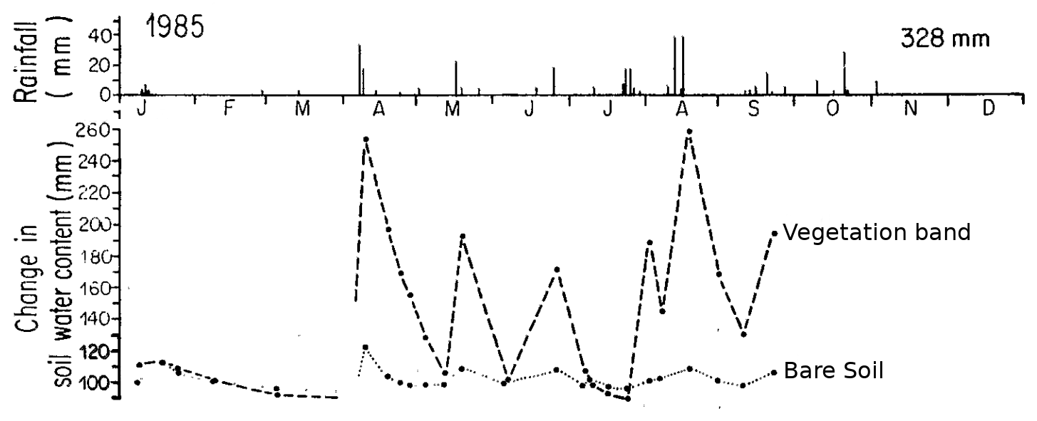
During rainfall events biomass feedback on infiltration acts to increase soil moisture where plants are by allowing surface water to enter the soil at a higher rate relative to the bare soil regions [15, 11]. However, soil moisture may be lost faster where biomass is present because of transpiration. While time-resolved soil moisture data at sites that exhibit banded vegetation is limited, the work of Cornet et al. [12] provides a time series of soil water content for a vegetation band and the bare soil region just uphill at a site in the Chihauahuan Desert for 1985. In data from [12], after rain events, the soil water content within the band increases dramatically relative to that of the bare soil, as shown in Fig. 2. It is only after extended periods without rain that the soil water content within the vegetation band becomes comparable, or even slightly below, the soil moisture of the bare ground. Even with these fluctuations, it appears from Fig. 2 that the soil moisture is, on average, more concentrated in the vegetation bands than in the bare soil regions. Qualitatively similar features occur for a site with banded vegetation patterns in Niger [36]. Data on gapped patterns collected by Barbier et al. [37] also indicates increased soil moisture levels in vegetated regions, although the shorter-timescale dynamics are qualitatively different. More comprehensive field studies would determine if similar observations occur at additional sites beyond these observational studies, and over longer time-periods. Many predictions from models are inconsistent with these observations of soil moisture distribution.
Conceptual reaction-advection-diffusion models can make qualitative predictions about the system over century timescales or longer. Such long-time simulation results ensure that the asymptotic behavior of the model is captured, and not just transient behavior that may be sensitive to the choice of initial conditions on biomass distribution. While these conceptual models typically encode a separation of scales into the advection and diffusion terms to capture slow biomass dispersal and fast water transport, the reaction terms associated with local ecohydrological processes are typically formulated on the slow biomass timescale. Because these models do not resolve individual rain events, the resulting predictions are interpreted as those of the annually averaged system, and therefore miss important details about soil moisture on shorter timescales.
The simplest of these conceptual models lump processes associated with surface and subsurface hydrology into a single “water” field, leading to a pair of reaction-advection-diffusion equations that captures interactions between biomass and water. Such “two-field” models, exemplified by Klausmeier [28], predict the highest concentration of water in the regions of bare soil between the vegetation bands. So-called “three-field” reaction-advection-diffusion models separately track the dynamics of surface and soil water, in addition to the biomass field. These models predict the soil moisture, on average, will peak within the biomass for typical parameter choices [22, 23]. However, it has also been shown, in the context of the three-field model by Gilad et al. [22], that the soil moisture spatial profile can be either in or out of phase with the spatial profile of biomass [38], depending on which mechanism for pattern formation dominates. While such models are capable of qualitatively capturing annually averaged dynamics observed in Fig. 2, they fail to provide useful predictions on shorter timescales.
Detailed mechanistic ecohydrological models for general water-limited environments [26], which capture processes on the fast time scales of individual rain events, have also been used to study the banded vegetation patterns. Such models predict that soil moisture can switch between being more highly concentrated under the vegetation bands to being more highly concentrated in the bare soil region for extended periods of time (a year or more). In these models, decadal time-averaged soil moisture is more highly concentrated in the bare soil region [27]. The annually averaged predictions of these models, like those of the Klausmeier model, are in contrast with the measurements shown in Fig. 2. Moreover, the complexity of such models limits numerical simulations to timescales of a few decades or less, and prohibits detailed exploration of the extensive parameter space.
Any prediction that soil moisture is, on annual average, more concentrated in the bare soil region, is inconsistent with the limited time-series data that is available for vegetation patterns [12, 36, 37]. Because of competition between increased infiltration and increased transpiration at vegetation bands relative to the bare soil regions, modeling choices about biomass growth based on plant physiology may play an important role in predictions about soil moisture distribution [39]. While we focus on the modeling of hydrological processes at appropriate timescales in this work, we expect that a critical analysis of model details of biomass dynamics, especially combined with more field measurements, could provide additional insights.
3 A three-field coupled timescale model
Before introducing the fast-slow switching model, the main focus of this study, we first present a reaction-advection-diffusion model in Section 3.1 with a seasonally-varying precipitation input that captures processes across the relevant fast and slow timescales. This ‘three-field coupled timescale model’ provides motivation for the switching model, and we discuss how parameters are chosen in Section 3.2. In Section 3.3, we explore the linear stability of the spatially uniform states within the seasonal model. Using a dimensionless version of the coupled model (Section 3.4) we demonstrate that the separation of timescales leads to a small parameter. The fast and slow systems that comprise the switching model are introduced in Section 4 by considering the limit in which this small parameter approaches zero. While the coupled model motivates the switching model, we treat the switching model as distinct from the coupled model instead of considering it as a means to approximate solutions of the coupled model.
3.1 Motivation: A three-field coupled timescale model
We first consider a model in which we input a time-dependent precipitation uniformly on a one-dimensional spatial domain. The model evolves a biomass field (), a soil moisture field , and a surface water height (). In restricting the description to these three dynamical variables, the model has its roots in the three-field conceptual reaction-advection-diffusion models of Rietkerk et al. [23] and Gilad et al. [22]. However, those models typically evolve the system on the timescale of biomass and input the rain at a constant rate given by the mean annual value. Although the basic structure of those models is a starting point for ours, we make modifications to capture details of the hydrological processes on the timescales at which they occur.
We will refer to our version of the three-field model as a “three-field coupled timescale model” or simply “coupled model” in this paper. It takes the following form:
| (1a) | ||||
| (1b) | ||||
| (1c) | ||||
where the infiltration rate of water from the surface into the soil is given by
| (2) |
This empirical infiltration model captures feedback from biomass, surface water and soil saturation in a highly simplified way as compared to more physical-based approaches that rely on modeling the vertical distribution of soil moisture [40]. Such simplified approaches have proven successful in other contexts [41].
In the next section, we describe each of the terms in the coupled model (1) to highlight differences from previous models and to justify our parameter choices which are summarized in Table 1. A summary of some of the most significant differences between the coupled model (1) and, for example, the Gilad et al. model [22, 42] are: Precipitation is time-dependent, there is no soil diffusion in the coupled model, there is no root augmentation feedback in the coupled model, there is biomass feedback on surface water transport in the coupled model and, in the coupled model, the infiltration slows as soil moisture saturates and becomes independent of surface water height for large enough surface water height.
3.2 Choosing Parameters
| parameter | units | default value(s) | description |
|---|---|---|---|
| 500 | infiltration rate coefficient | ||
| – | 0.1 | bare/vegetated infiltration contrast | |
| 0.1 | Biomass level for infiltration enhancement | ||
| 1 | infiltration rate -independent for | ||
| – | 4 | infiltration exponent (soil moisture) | |
| – | 0.005 | elevation grade | |
| – | (or 1)∗ | surface water transport exponent | |
| (or )∗ | surface water transport coefficient | ||
| 20 | surface roughness coefficient | ||
| biomass diffusion | |||
| soil water capacity | |||
| 0.2 | evaporation rate | ||
| 0.67 | transpiration coefficient | ||
| 4 | biomass carrying capacity | ||
| 0.1 | water use efficiency coefficient | ||
| 0.01 | biomass mortality rate |
Surface Water Transport
We take the Manning formula for gravity-driven open channel flow [43, 44] as a basis for our surface water transport model. According to this formula, the average velocity of the fluid in a wide channel is empirically determined to be , where characterizes the surface roughness, is the local elevation grade and is the height of the water. By modifying the surface roughness term based on literature values for vegetated surfaces and bare soil, we include the influence of biomass on runoff interception leading to a slow-down in the surface water speed within vegetated regions. In particular, we take the water flow speed to be given by
where the term allows us to describe the change in surface roughness from bare to vegetated soil. The value of the exponent that is consistent with the Manning formula corresponds to . With and a typical value for the elevation grade of (i.e. an grade) we estimate the remaining parameters using Manning roughness coefficients [43, 44]. Typical values of for bare soil ( ) and dense vegetation ( ) lead to and . Estimations using a typical surface water height around result in the same values of (note different units) and when using . These values and surface water when lead to a water velocity of around on bare soil and just over a factor of 10 slow down through vegetation with biomass value . While the value of the exponent that is consistent with the Manning formula is , we take for most of the results in Section 5 for computational convenience. This makes the water flow speed independent of and the advective transport term in Eq. 1a linear in the surface water height . (We present some numerical calculations and simulations with in Fig. 3(a), Fig. 11, and Fig. A3; our limited exploration shows results that are similar when is replaced by .)
Soil Moisture Dynamics
We use a “bucket model” that tracks a depth-averaged soil moisture within the plant rooting zone according to the soil moisture balance equation (1b), where is the relative soil moisture [45]. Denoting the rooting depth by and the soil porosity by , the quantity represents the volume of water contained in the root zone per unit ground area, and has units of column height. In the model here, we assumed typical values of and [45]. Water enters the soil from the surface via the infiltration model (2) and is lost through evapotranspiration as . The linear evaporation rate coefficient is set so that the evaporation rate is approximately when soil moisture is at , which is approximately the field capacity [45]. We neglect the shading effects on evaporation by making the evaporation rate independent of biomass . We set the transpiration parameter to be in order that the transpiration rate with biomass density reaches approximately when soil moisture is .
We take a heuristic approach to modeling infiltration, similar to those of previous conceptual models [46, 22]. The parameter in Eq. 2 represents an effective infiltration rate, which was here assumed equal to in order to ensure typical values of the infiltration rates, e.g., in the numerical simulation. We note, however, that the value of depends on the soil type. Similar to previous models, we assume a factor reduction in infiltration when biomass levels fall far below the threshold value of . This biomass feedback models the presence of a soil crust that reduces infiltration in bare soil and root systems that enhance infiltration in vegetated areas. We additionally assume that the infiltration rate becomes independent of surface water height for significantly greater than , where (many descriptions of infiltration have this -independence, see e.g. [25]). . Finally we include a factor of with to account for the reduced infiltration values as the moisture content reaches saturation. While soil saturation effects are typically negligible for the case of constant precipitation, we are interested in considering large, concentrated rain events where the soil moisture can increase dramatically in a very short time.
We neglect subsurface water flow, under the assumption that surface water flow will be the dominant mode of water transport. In other models, subsurface transport has been included as linear diffusion but we do not notice significant differences in the limited simulations where we have included it (see A of the online supplement for more details). We also neglect leakage of water from the root zone to deeper areas for similar reasons: it did not have a large impact on the limited simulation results where we have included it. However, a more comprehensive exploration of the role of these two subsurface soil processes, and how they are modeled, could provide a more detailed understanding of when they can and cannot be neglected.
Biomass Dynamics
We leave the biomass dynamics largely unchanged in form from a simplified version of the model by Gilad et al. [42]. The plant growth rate is taken to be proportional to transpiration rate , except with a logistic term that can be thought of as capturing a decrease in water use efficiency as biomass increases. Specifically, the growth term is , where the proportionality constant is set by the typical water-use efficiency for plants. Increased biomass begins to significantly decrease growth rates when , where we take (however, biomass levels stay well below in all simulations presented here). One notable difference from the biomass growth term of the Gilad et al. [42] model is that we do not include a root augmentation feedback associated with the lateral spreading of roots. Mortality is modeled by linear loss with coefficient , which was estimated by Mauchamp et al. [47] using typical carbon maintenance costs.
We model seed dispersal by linear biomass diffusion with rate . This parameter is often chosen in models of this type without clear justification; ranges from in Gilad et al. [42] to in Klausmeier [28] to in Rietkerk et al. [23]. (It may ultimately have been chosen to help the model match pattern characteristics; see discussion in Gandhi et al. [48].) Our linear stability results, presented in Fig. 3, show that this parameter, for our model, controls a cut off for short-wavelength linear instabilities of the uniform state within the seasonal model. While this parameter is unconstrained and diffusion is likely a poor model of seed dispersal, we make no adjustments to in our simulations, leaving it fixed at a value of . We note that this model does not attempt to capture drought resistant behavior that plants in dryland ecosystems are known to exhibit. Nor does it include transport of organic material or seeds via water during rain storms.
3.3 Spatially uniform states and their stability
If we were to set the precipitation rate to a constant, , then we could explicitly determine two possible types of spatially uniform steady state solutions of (1). One is the bare soil state, defined by , and with
| (3) |
which exists for all . This trivial solution becomes unstable at a transcritical bifurcation point , and for , there also exists a uniform vegetation solution with nonzero biomass
| (4) |
We find that these two uniform solutions, and the associated transcritical bifurcation at , carry over to the case that the precipitation comes into the system during equally-spaced rain events per year. We consider rain events with constant precipitation rate (), each of duration . Specifically, if we denote the Heaviside unit step function by , and we let
| (5) |
then a periodic seasonal rainfall is obtained by repeating this pattern, i.e. by letting . The total annual precipitation is , and it plays the role of a mean annual precipitation rate in our investigations. For the default parameters given in Table 1, the transcritical bifurcation occurs when the total annual precipitation is , and we find that this value does not change when we use the pulsed, periodic rain input (5) rather than constant precipitation .
The stability of the spatially-uniform vegetation state to heterogeneous perturbations is determined by computing Floquet multipliers associated with the linear variational equations, given perturbations proportional to (See, e.g., the book by Meiss [49]). Specifically, we let
where is a spatially-uniform, temporally periodic solution of (1) for the periodic rain input (5). In practice, we compute by integrating the ODEs associated with spatially uniform states of (1) forward in time until the system converges sufficiently close to this stable periodic orbit. For the linear stability calculation, we linearize in the perturbations , and (numerically) compute the Floquet multipliers as eigenvalues of the associated Monodromy matrix . This calculation is carried out on a two-dimensional grid of values for mean annual precipitation () associated with Eq. 1 and the wavenumber of the perturbation. The stability boundary in the parameter plane is then determined by interpolating where the leading Floquet multiplier crosses the unit circle; we refer to the instability region in the -plane as the “Turing-Hopf bubble”. (See B of the online supplement for more details of the linear stability computations.)
Results of some of our numerical computations of the Turing-Hopf bubble are presented in Fig. 3. In each of figures (a)-(d) the red Turing-Hopf bubble is the reference one. It was obtained using the default parameters of Table 1 with overland water transport exponent ; the precipitation function Eq. 5 had and . This means that there were two big rain events per year, separated by six months (two rainy seasons), and each lasted for six hours. Here we summarize the findings from our linear stability calculations.
-
1.
Figure 3(a) shows that increasing the exponent from to leads to a slight decrease in the size of the Turing-Hopf bubble. Most of our simulation-based investigations incorporate as taking significantly increases computation time.
-
2.
Figure 3(b) shows the impact on the instability region of changing the duration or frequency of the rain events. With constant rain input the instability region is significantly greater as shown by the large blue Turing-Hopf bubble that extends all the way to . Alternatively, if we keep the intensity of rain the same but decrease the frequency from two rain events per year to just one rain storm, the instability region shrinks quite significantly to the small yellow Turing-Hopf bubble. This suggests that the MAP level at onset of instability of the uniform state decreases as rain events become less frequent. In fact, if we decrease the frequency of large rain events to one every 2 years, then there is no pattern-forming instability of the uniform state for these parameter values.
-
3.
Figure 3(c) shows how the transport parameters and in Eq. 1 impact the shape of the Turing-Hopf bubble. While there is an instability of the uniform state even when we neglect biomass diffusion (), there is no short-wavelength (high ) cut-off as indicated by the asymptotically vertical boundary to the blue region at . As increases to we find that the short-wavelength modes are stabilized. The long-wavelength boundary is apparently set by the overland transport parameter , as suggested by the change of shape of the Turing-Hopf bubble when is decreased by an order of magnitude to .
-
4.
Figure 3(d) shows how the Turing-Hopf bubble changes when one of the two biomass-hydrology feedbacks is shut off. The () Turing-Hopf bubble is quite similar in shape, although smaller, to that for (). By way of contrast, the shape of the Turing-Hopf bubble with only the transport feedback (i.e. when ) is more circular, with an expected wavelength of pattern that is smaller than that when the infiltration feedback is turned on.
The Turing-Hopf bubbles in Fig. 3 indicate regions of linear instability of the uniform vegetation state. They are not equivalent to the regions of stability of nonlinear patterns which are typically referred to as “Busse balloons” [50]. Even still, the numerical simulation results presented in Section 5 suggest that these linear calculations provide some insight into characteristics of fully nonlinear states.
3.4 Non-dimensionalization: origin of the small parameter
We now introduce a rescaling of the three-field coupled timescale model Eq. 1 to put it into dimensionless form. The scaling for time is chosen based on the infiltration timescale which corresponds to the characteristic time for a surface water column of height to infiltrate into the soil under optimal conditions: large reservoir of surface water, dense vegetation, and dry soil. for the parameter values of Table 1. In contrast the characteristic time associated with maximal biomass growth within this model is , which corresponds to for our default parameters. The spatial scale is chosen based on the characteristic advection distance of surface water before infiltrating into the soil . This distance is for our parameters. Biomass is scaled by and surface water height by . For this choice of scalings, namely,
the coupled model (1) becomes
| (6a) | ||||
| (6b) | ||||
| (6c) | ||||
where
and the dimensionless parameters are defined in Table 2. The parameter represents the ratio of the infiltration timescale to the growth timescale and is of order . We exploit the smallness of this ratio in the following section to motivate the switching model that is the focus of the rest of the paper.
| parameter | definition | value |
|---|---|---|
| 80 | ||
| – | ||
| – | 0.1 | |
| 0.025 | ||
| – | 4 | |
| 0.037 | ||
| 0.11 | ||
| 1.48 | ||
| 0.15 | ||
4 A fast-slow switching model
Rainfall initiates fast hydrological processes associated with overland waterflow and, with it, infiltration from the surface into the soil. These processes occur on timescales of minutes to hours. Evapotranspiration and plant growth occur on much longer timescales, days to months, and we assume can be neglected during rain events. This separation of scales is evident in the coupled model presented in Section 3 from the small parameter in Eq. 6 which represents the ratio of the water infiltration timescale to the biomass growth timescale . In this section, we present a switching model that captures dynamics of fast processes initiated by rainfall and switches to the dynamics of slower processes in the absence of surface water. Figure 4 shows a schematic diagram of such a model, which we describe in detail in Section 4.1. We then, in Section 4.2, discuss numerical methods employed to explore the model along with some potential issues associated with our choice of periodic boundary conditions.
4.1 Fast-Slow Switching Model: exploiting the limit
We now motivate a switching model for banded vegetation patterns by leveraging the fact that in the dimensionless model Eq. 6. We first consider the case that , corresponding to the assumption that the dynamics occurring on the biomass growth timescale are completely negligible. The assumption leads to a fixed biomass profile since from Eq. 6c. The remaining two equations of system (6) become:
| (7a) | ||||
| (7b) | ||||
We refer to Eq. 7 as the “fast system,” which models the dynamics during and shortly after rain events. (For convenience, we substituted in the expressions for infiltration rate and transport speed that are defined below Eq. 6.)
We start evolution of the fast system when a rain event begins, and continue until the surface water becomes negligible, i.e. below a threshold of order . We expect these fast dynamics to occur over an hours timescale, after which we obtain an updated soil moisture profile
| (8) |
that has been replenished by the rain event. The profile of the soil moisture replenishment term is determined by the fast system (7), and depends on the biomass and soil moisture profiles prior to the rain event along with the rain event itself.
The fast dynamics of Eq. 6 are terminated once , after which the soil moisture and biomass evolution proceeds on a slow timescale given by under the assumption that the surface water height remains fixed at . Rescaling time in Eqs. 6b and 6c then leads to
| (9a) | ||||
| (9b) | ||||
We refer to Eq. 9 as the “slow system” and use it to evolve biomass and soil moisture in the absence of surface water. The slow system (9) is initialized with the biomass profile prior to the rain event and the replenished soil moisture , and evolves until the next rain event occurs. In results and discussion sections that follow, we numerically explore this fast-slow model that has been motivated by the coupled model (1).
4.2 Numerical methods and boundary conditions
We discretize in space with finite differences using first-order upwinding for advection and second-order centered differences for diffusion. For time integration we employ Matlab’s ode15s, an implicit variable-order solver designed for stiff equations [51]. At the start of each rain event, the fast system is initialized with the output biomass (which will remain fixed), soil moisture of the slow system and no initial surface water. The fast system is run for twice as long as the rain event, with a constant rain input for the first half of this time. The surface water height typically has fallen to below by this point, and the simulation proceeds to the slow system initialized with the updated soil moisture and previously output biomass. However, if the surface water is not below a threshold value of , the fast system is run again with no rain input for fixed intervals of time until the threshold is reached and the simulation can move on to the slow system.
The simulations are carried out on a periodic domain that typically corresponds to a few wavelengths of the banded pattern. The underlying assumption for this choice of boundary conditions is that we are considering a small section in the middle of a very long hillslope. One potential issue that may arise with periodic boundary conditions is that, during the fast system, surface water may repeatedly reach the bottom of the domain and get re-injected at the top of the domain. We don’t expect surface water to travel more than a few vegetation bands before infiltrating into the soil, and find that our simulations are consistent with this expectation. For example, a simulation of the fast system (7) with parameters from Table 1 shows that 2 of surface water at the top 15 of a hillslope is decreased to approximately 1% of its original amount after traveling through an 80 wide band of vegetation with peak biomass value of . The water travels with a speed of approximately through the vegetation band and 13 over the bare soil. This simulation, which is shown in Fig. 5, is initialized with the state reached just prior to a rain event at 200 from the simulation shown in Fig. 8 of Section 5.2.

5 Numerical results for fast-slow model
In this section, we explore pattern formation within the fast-slow switching model, Eqs. 7 and 9, through numerical simulation. Inspired by the biannual rainy seasons shown in Fig. 1(b), we take as a base-case scenario two major rain events each year, spaced six months apart, with a mean annual precipitation of 160 . In this case, each rain event lasts for six hours, and deposits half of the mean annual precipitation at a constant rate during that short time-frame. Unless otherwise noted, we use parameter values from Table 2 with , corresponding to dimensional quantities given in Table 1, throughout this section. We also report all quantities in dimensional units, with the conversions described in Section 3.4. (See also parameters in Table 1.)
We first study characteristics of stable periodic solutions obtained using sinusoidal perturbations of the uniform state as initial conditions in Section 5.1. These solutions provide a basis for interpreting the results of simulations initialized with random initial perturbations, which we discuss in Section 5.2. We provide a detailed picture of transients that persist on ecologically relevant timescales, e.g. decades to centuries, for this case and describe the observed model behavior on the timescale of millennia. We then, in Section 5.4, study the influence that the amount of rainfall has on pattern characteristics. Finally, in Section 5.5, we explore the role that biomass feedback plays in infiltration and surface water transport in the pattern forming process. Additional supporting simulation results are reported in A of the online supplement.
5.1 Stable periodic states
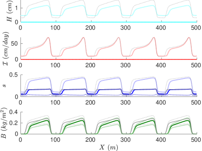
We consider a spatial domain of length and take the positive -direction to be uphill. We initialize the fast-slow system with a 1% sinusoidal perturbation of wavenumber , , to the uniform solution with constant precipitation given by Eq. 4. For , the simulation converges to a periodic traveling wave solution with wavenumber , and for the simulation converges to a periodic pattern with different wavenumber (typically with ). These stable wavenumbers correspond to a stripe spacing from () all the way to the size of the domain (). Figure 6 shows examples of spatial profiles of two different wavenumber solutions for the fixed parameter set considered here. The solid line in each plot represents the annual average while the dotted lines indicate the pointwise maximum and minimum. The average biomass, the surface water and soil moisture all peak at the leading edge of the vegetation bands. While the surface water and infiltration rates are near zero on average, the maximum values are at around 2 and , respectively, during rain events. The soil moisture within the vegetation bands also varies significantly in time, going from just after a rain event to below 0.05 just before the start of the next one. The seasonal variations in biomass, on the other hand, are less dramatic. We note that, during rain events, the surface water height is expected to decrease in the vegetated regions for flat-terrain patterns because of increased infiltration [25]. However, on a hillslope, the flow induced by the elevation gradient along with the increased surface roughness of vegetation leads to an increase in predicted surface water height within the vegetation bands in the fast-slow model.
Figure 7 indicates that many pattern characteristics (e.g. average biomass, fraction of wavelength covered by vegetation) show remarkably little variation with respect to wavenumber. Panel (a) indicates a monotonic decrease in the maximum biomass value as a function of wavenumber. The fraction of the wavelength with vegetation cover, shown in Panel (b), varies little with , on the order of 5% with a maximum at around . To compute the fractional cover, we take the edges of the vegetation band to be the points of steepest increase/decrease in biomass. Using a threshold value of to define the edges leads to nearly identical fractional cover values.
Unlike the average biomass and fractional cover, the average migration speed of the bands does vary significantly with wavenumber: it decreases monotonically from about 200 for the largest band spacing of ( ) to about 10 for a small spacing of ( ), and has a value of for patterns with a wavelength of 100 . As a possible reference point, observational studies of banded patterns in the Horn of Africa record typical wavelengths of and migration speeds measured in 10s of centimeters per year, on slopes with typical elevation grades %. [5, 52, 53]. The model predictions are therefore of the right order of magnitude, and this is without these characteristics being a factor in our parameter selection.
Since there is a significant (increasing) trend in migration speed with wavelength, we choose to plot the migration frequency (wavelengths of the pattern per century) in Fig. 7(c). For this we find a relatively modest range of /century with a peak speed for a wavelength of 100 . Deblauwe et al. [5], drawing on pattern observations around the globe, report slightly smaller mean migration speed values in the range of /century, although with error bars that can bring these to our higher range.
We note that predictions of wavelength and migration speed that are based on a constant rain input to the coupled model (1) are way off, both in comparison to the reported observations and to our fast-slow simulations that incorporate short rain events. For instance, the onset of Turing patterns for a constant rain input have wavelength of 26 , and travel rapidly at a speed of 3.5 (i.e. wavelengths per century). Moreover, the associated Turing-Hopf bubble of Fig. 3(b) extends all the way to a , giving a rather high lower bound to where patterns would occur. Using linear predictions from the case of constant rain input, and trying to adjust the parameters to fit those observed pattern characteristics, would lead to different parameter choices.
5.2 Random initial conditions and asymptotic behavior
While the periodic states summarized in Figs. 6 and 7 persist for at least 5000 years and are stable to small perturbations, long-time simulations with random initial perturbations eventually approach the long-wavelength patterns. We first provide a detailed account of long-lived transients that persist on ecologically relevant timescales of centuries before discussing this asymptotic behavior on the scale of millennia.
Figures 8, 9 and 10 show details of a 200-year simulation on a 500 domain with mean annual precipitation of . These are the same parameters we used for the periodic patterns in the previous section. However, we modify the initial condition to be a 1% random perturbation of the uniformly vegetated state that’s obtained for constant precipitation, given by Eq. 4. These values, and , are a good estimate for the mean of the uniform state in the seasonal case. A spacetime diagram of the annually-averaged biomass along with spatial profiles of the surface water, infiltration rate, soil moisture and biomass during the last year of the simulation are shown in Fig. 8.
The simulation evolves the fast system, Eq. 7, during and shortly after each rain event. Specifically, constant precipitation, at a rate of about 13 , is input during the first six hours and none during the next six hours, during which time the surface water height drops to below . The biomass profile, which remains fixed during this time, is shown in Fig. 9(a). Figure 9(b) shows the initial and final soil water content in units of . A total of 8 of water is input uniformly across the domain by the rain storm and the vegetation bands collect approximately 10.6 on average, while the bare soil regions collect approximately 1.7 on average. The vegetated regions therefore absorb, on average, approximately 6.2 times the amount of rainfall because of runoff from the bare soil regions. Figure 9(c,d) show spacetime diagrams for surface water height and instantaneous infiltration rate over the 12 hour period that the fast system is run. During the rain, both the surface water height and the infiltration rate are enhanced by the presence of biomass. The surface water is increased in the vegetation bands because increased surface roughness slows water transport. This increased height, along with a positive feedback of biomass directly on infiltration rate, lead to the heightened accumulation of soil water content in the vegetation bands that is seen in Fig. 9(b).
At the end of the 12-hour period of the fast system, we then initialize the slow system with the updated soil moisture from the fast system and the same biomass profile. Figure 10 tracks soil moisture and biomass at locations in the vegetation band (blue and green) and in bare soil (orange) over time for the slow system during the final year of the simulation shown in Fig. 8. The soil moisture in the vegetation band initially increases significantly, but eventually falls to nearly the same level as the bare soil just before the next rain event. The biomass peak is delayed by approximately two months after the rain event.
While the behavior in Figs. 8, 9 and 10, initialized with random perturbation, persists for a millennium, 3500-year simulations (see Fig. A2) reveal it to be transient. This is in contrast to the cases where a periodic perturbation of specific wavenumber is introduced, as described in Section 5.1. The periodic states in Figs. 6 and 7 persist as traveling wave solutions (on annually averaged timescales) for at least 5000 years.
The long transients persist on ecologically relevant timescales and have wavelengths consistent with predictions from linear stability analysis of the coupled model, Eq. 1, with identical rain input (i.e. six-hour constant rain intensity storms every six months). Those calculations indicate an onset of the pattern-forming instability occurs for a total annual rain of (input in two large rain events), and are associated with a wavelength of . For mean annual precipitation of , the “Turing-Hopf bubble” has a width that indicates the uniform state is unstable to perturbations with wavenumbers between and , corresponding to wavelengths greater than and all the way up to a kilometer scale; the most unstable mode for these conditions occurs for (a wavelength of ), where the Floquet multiplier reaches a peak value of . Simulations of the fast-slow system on a 500 m domain, with an initial periodic perturbation of fixed wavenumber within this Turing instability range, appear to be stable, at least for wavelengths greater than , i.e. they do not undergo band-merging events on the millennial simulation timescale. (See results presented in Fig. 7.)
5.3 Nonlinear dependence of transport on surface water height
The theory for open channel flow suggests a nonlinear dependence of surface water height on transport, e.g. in Eq. 1a. However, we use out of numerical convenience for the majority of simulations presented here in Section 5. The predictions of the linear theory for the three-field coupled model presented in Fig. 3(a) show relatively modest differences between the and cases. The linear theory, however, is about the stability of the spatially uniform solutions and does not provide information about the fully nonlinear states. Our limited simulations suggest that the nonlinear behavior may also be qualitatively unchanged for , compared to . To illustrate the minor quantitative differences in periodic solutions for the two cases, we take the solution with for the case of , shown in Fig. 6(b), as an initial condition for a simulation with . A comparison of this initial condition to the final state that the simulation converges to is shown in Fig. 11. The resulting periodic state exhibits slightly less biomass for : the bands are slightly narrower with slightly lower peak values. Despite these minor quantitative differences, the overall qualitative character of the solution profiles is the same. (Another example, presented as Fig. A3 in A of the online supplement, starts with a random perturbation of the uniform state, and shows a much slower development of patterns for , indicating another aspect of the numerical speed-up we achieve for .)
5.4 Dependence on mean annual precipitation
In this section we explore the impact on the patterns of ramping down the mean annual precipitation and then ramping it back up, with details on our protocol for this provided below. We find that the range of existence for patterns is considerably greater than suggested by the linear theory of Section 3.3; rather than patterns only existing in the range of , they exist as highly nonlinear states in the range of . We also find that on gradually decreasing the precipitation there are a number of discrete steps that reduce the number of bands on the domain until only one band persists. However, as we then increase the precipitation, these jumps in the number of bands do not reverse themselves. Instead the single band persists but with ever increasing width until it eventually fills the domain as a spatially uniform vegetation state. We find that the average biomass decreases approximately linearly with precipitation level, but that the peak biomass values in the bands are relatively constant. In particular, it is the fraction coverage per wavelength that contributes most significantly to the change in average biomass on the domain, and not the peak biomass level in the bands.
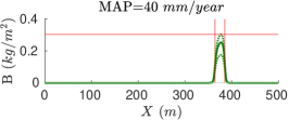
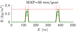
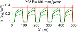


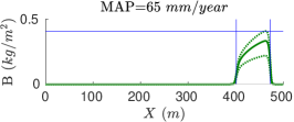
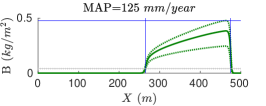
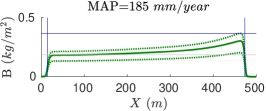

Results associated with decreasing mean annual precipitation are summarized in Fig. 13. In order to determine where the uniform state loses stability, we begin with the stable uniform vegetation state at 240 and decrease the precipitation amount in steps of 2 . At each step, we add 1% perturbations and allow the simulation to run for 300 years (or shorter if it converges to a uniform state more quickly). We find that the uniform state of the fast-slow system remains stable until . Perturbing the uniform state at with 1% sinusioidal perturbations of wavenumber with , we find that the uniform state is unstable to the wavenumbers, corresponding to wavelengths between about 63 and 167 . This is quantitatively consistent with the predictions of linear theory for the three-field coupled model presented in Section 3. Interestingly, the average biomass on the domain for these highly nonlinear patterned states is approximately equal to the maximum biomass obtained for the uniform vegetation state.
We continue decreasing the mean annual precipitation from , in steps, starting with the wavenumber pattern, corresponding to a wavelength of 100 . This state persists until the precipitation reaches 52 , well below the transcritical bifurcation that creates the uniform state at 109 . Moreover, the patterned state sustains more biomass on average than the uniform state, for precipitation values where the uniform state does exist. While the patterns maximum biomass value does not change very much over this range, the fraction of the domain covered by vegetation decreases linearly with precipitation, i.e. there is a linear decrease in the width of the vegetation bands with . At 52 , a pattern with 250 wavelength emerges from the simulation and transitions to a single band on the 500 domain at 40 . This so-called ‘oasis state’ finally collapses to the bare soil state at 34 .
As shown in Figure 13, we also scan up in precipitation, starting with the oasis state at 35 and moving in increments of 2 as before. This state with a single vegetation band on the domain persists all the way up to 201 before loosing stability to the uniform vegetation state. As the precipitation increases, the width of the vegetation band increases. We note that at around 179 , there is a qualitative change in the shape of biomass profile, in terms of its concavity. Above 179 , the biomass values at the trailing edge of the vegetation band correspond to those of the uniform vegetation state for the given precipitation level. If we again decrease precipitation, starting now with a one-pulse solution, we find an apparent bistability of two distinct single-pulse states for precipitation between approximately 175 and 177 , which is in a region where the uniform state is also (barely) stable. See Fig. A4 in A of the online supplement for more details.
5.5 Influence of biomass feedback on infiltration and transport
The fast component of our model (7) incorporates two important feedbacks between the biomass and the water resource re-distribution, and in this section we explore the relative impact of those feedbacks on the pattern characteristics. The presence of biomass is known to enhance infiltration of surface water into the soil within the dryland ecosystems that exhibit banded vegetation patterns. This positive feedback plays a central role in the pattern formation process within many conceptual models [22, 28, 46]. The model we consider here captures an additional feedback of biomass on the hydrology, namely an increase in surface roughness that can slow down water flow where biomass is present [24, 25]. Our standard choice of parameters includes both kinds of biomass feedback but, as Fig. 14 illustrates, patterns are possible with either feedback alone. These results are consistent with linear predictions from the three-field coupled model shown in Fig. 3(d).
The simulations for Fig. 14 are initialized with a random perturbation of the uniform state, and carried out with mean annual precipitation of 140 . The parameters characterizing the biomass feedback on surface water transport, in Eq. 1a, and infiltration rate, in the infiltration function in Eqs. 1a and 1b, are varied with all other parameter values taking the default parameters from Table 1. Simulation results with the standard parameters, and , are shown in Fig. 14(b). These results are to be contrasted with those of columns (a) and (c) for which either the transport or the infiltration feedback is turned off by setting or , respectively. The top row shows plots of the spatial profiles of surface water, infiltration rate, soil moisture and biomass during the last year of the simulation. The middle row shows spacetime diagrams of the annually-averaged biomass. The bottom plots show time series of the soil moisture at the peak biomass location within the vegetation band (blue) and in the center of a bare soil region (orange) during the last year of the simulation. The soil moisture plot provides a qualitative comparison for field measurements, as shown in Fig. 2.
We make the following observations about Fig. 14:
-
1.
While the width of the bare soil region is somewhat comparable between all three cases, the widths of the vegetation bands are significantly greater when there is no feedback in the transport, i.e. . This leads to far fewer bands on the domain in this case, compared to the cases with transport feedback.
-
2.
In absence of the infiltration feedback i.e. , the bands are more regular in spacing and travel approximately twice as fast across the domain and with uniform speed. In contrast, when there is no transport feedback, i.e. , then we see a lag between the leading edge colonization and trailing edge death.
-
3.
The asymmetry in the profiles of the vegetation bands, between leading uphill edge and trailing downhill edge, is much more pronounced in the presence of the transport feedback. In fact, the profiles are almost triangular when the infiltration feedback is turned off, and almost rectangular when there is no transport feedback. This difference in profiles is also quite pronounced in the soil moisture profiles.
-
4.
The transport feedback is required to concentrate the surface water in the bands. Morever, the peaks of the surface water are lower without an infiltration feedback, and greatest when both feedbacks are present.
-
5.
The time series of the soil moisture in the lower plots shows then when there is no infiltration feedback there is a decreased contrast in soil moisture between the bare soil and vegetation band immediately following the rain event.
-
6.
When there is no infiltration feedback the soil moisture at the peak of the biomass actually falls below the soil moisture in the bare soil zone. Specifically, a switching point at around 100 days after the rain event is seen in the time series of the soil moisture, where of the bare soil becomes higher than within the vegetation band. This switching behavior is also observed in some drought phases of the field observations illustrated by Fig. 2.
6 Discussion
In this paper we have motivated and then investigated a fast-slow mathematical modeling framework, Eqs. 7 and 9, for vegetation pattern formation. This fast-slow framework exploits the inherent separation of timescales between fast hydrological processes and slow biomass dynamics. Our fast-slow model switches between a fast system, Eq. 7, that resolves aspects of the surface water and soil moisture dynamics during rain events at the fast timescale of minutes to hours, and a slow system, Eq. 9, that captures the dynamics of biomass and soil moisture interactions on the slow timescale of weeks to months when no surface water is present. By modeling key processes on the timescales at which they occur, we are able to employ a conceptual-level model with parameter values that are consistent with observations of the processes being modeled. Soil moisture dynamics occur on the fast timescale, through infiltration, as well as the slow timescale, through evapotranspiration. A comprehensive set of appropriately resolved time series data on soil moisture for banded vegetation patterns would be useful to probe this modeling framework on its multiple timescales.
We do not choose parameters to fit predicted pattern characteristics to observations of banded vegetation patterns, as has been done for models that were developed for the slow timescale of the biomass dynamics alone (See, e.g. [37]). Even still, the fast-slow switching model is able to accurately capture certain details of the phenomenon with hydrologically-informed parameter values. Numerical simulation of the model reveals that the spacing of the vegetation bands, and their up-slope colonization speeds are of the right order of magnitude. Another focus of our investigation relates to the distribution of the soil moisture relative to the biomass. Our expectation, based on limited ground-based studies of this, is that the soil moisture should be trapped for much of the year where the biomass is located. Our simulation results are consistent with this. However, we make a number of simplifying modeling assumptions, including to neglect subsurface water transport and the influence of lateral spreading of roots. More careful thought must also be given to the biomass model in future work to ensure that their key processes are being captured.
Many model studies suggest that bare-soil areas should increase in size to compensate for a decrease in precipitation level [54]. The fast-slow switching model further predicts that whether this compensation occurs by adjusting the band spacing or the band width depends on whether the rainfall is increasing or decreasing. Our most extensive model simulation results focus on a situation where there are two heavy rain events of equal strength per year, which drive the pattern formation process. From those simulations, there is strong evidence for multi-stability, history-dependence, and hysteresis. In some of the longest simulations we gradually decrease and then increase the annual precipitation levels. As precipitation levels decrease, a gradual decrease in band width is observed. This narrowing is accompanied by occasional losses of bands leading to increases in band spacing. For low precipitation levels, the vegetation bands are narrow, with large swaths of bare soil in between them. As the precipitation level increases, the widths of the bands increase without any change to the wavelength of the pattern. These results are consistent with predictions suggested to Hemming by his detailed observations of banded patterns in Northern Somalia that he reported in 1965 [10]. In particular, he predicted that increasing rainfall might widen individual arcs while decreasing rainfall might reduce the number of arcs.
The fast-slow modeling framework is well-suited for exploring the impact that the temporal rainfall pattern has on spatial vegetation pattern formation in these ecosystems, and this will be a major focus of future efforts. Preliminary simulation results, which are described further in the online supplement, indicate that the temporal distribution of rain events influences whether patterns will occur at a given level of mean annual precipitation, but more work is needed to understand this in detail. With fewer rain events (at the same annual precipitation level), patterns occur within a smaller range. For one twelve-hour rain event each year, at our standard parameters (see Table 2), patterns occur at a range of to . With the same rain amount spread between two six hour events each year, the range grows to to (Fig. 13). A previous study by Guttal et al. [30] on the effect of seasonal rain input within the three-field model by Rietkerk et al. [23] found the opposite trend. However they did not attempt to incorporate timescales associated with individual rain events and instead focused on capturing the impact of drought on the biomass dynamics.
It may be tempting to interpret the presence of patterns as a sign of stress in the ecosystem, with their existence at higher levels indicating reduced resilience. However, we caution against this. In the fast-slow model presented here, the patterned states have a higher total biomass than the corresponding uniform vegetation state for the same precipitation level. In our ramped precipitation simulations summarized by Fig. 13, we find that the pattern state only disappears (around 201 ) when it’s no longer “an advantage” to the system over the uniform vegetation case.
While the fast-slow switching model is motivated by a small parameter in a three-field coupled timescale model, Eq. 6, we do not consider the fast-slow model as an approximation of the coupled model in the sense of singular perturbation theory. However we do show that linear predictions of the coupled model are consistent with simulations of the fast-slow model when the same temporal rain profile is used. The mathematical relationship between these two models will be explored at a more formal level in future work. Our goal is to be able to start from a more detailed model that captures fast hydrological processes and formally make the reduction to a two-field model that operates on the slow timescale. While this has been done in the high infiltration limit where there is no overland water flow [55], capturing the influence of surface water transport on soil moisture through an effective transport could help make a direct link to models like those of Klausmeier. Moreover, it may provide insight into how well rainfall is approximated by the inclusion of an additive constant to the soil moisture rate equation, as is commonly done, or suggest alternate approaches that may be more appropriate.
In future work, we are particularly interested in considering the influence of stochastic rainfall within the fast-slow switching framework. One approach for doing so, conceptually similar to the work of Siteur et al. [35], is to develop the interpretation that the fast system provides a kick to the slow evolution of soil moisture and biomass. The kicks from the fast system, under certain simplifying approximations, can be solved in closed form via the method of characteristics. This may lead to progress towards analytic insights as well as an increased speed-up of numerical simulations. Alternatively, numerical speed-up could be achieved by machine learning approaches [56], or by more parsimonious modeling of the fast system.
The fast-slow framework introduced in this paper is a conceptual model that captures the natural timescales of important processes. In particular, it resolves the fast hydrological processes that contribute important positive feedbacks between the biomass and the water resource.
It produces physically reasonable predictions in the absence of parameter tuning and provides a testbed for exploring the impact of different precipitation regimes on patterns. At a practical level, this framework’s advantage is two-fold: (1) capturing both the fast and slow timescales in the model allows for the parameters to be chosen based on information about the particular processes being modeled, and (2) separating fast and slow processes in a switching model provides a computational speed-up over a coupled timescale model. We also believe that there is a conceptual advantage in that the fast-slow switching framework captures the qualitatively different behaviors of the system when surface water is and is not present in a very transparent way.
Acknowledgements. The work by PG was supported in part by the National Science Foundation grant DMS-1440386 to the Mathematical Biosciences Institute. The research of MS was supported by NSF-DMS-1517416. PG and MS also benefited from participating in the wonderful birthday conference, Advances in Pattern Formation: New Questions Motivated by Applications, honoring Ehud Meron’s pioneering work in the field of pattern formation.
References
- [1] I. Noy-Meir. Desert ecosystems: environment and producers. Annu. Rev. Ecol. Syst., 4(1):25–51, 1973.
- [2] S. Schwinning, O. E. Sala, M. E. Loik, and J. R. Ehleringer. Thresholds, memory, and seasonality: understanding pulse dynamics in arid/semi-arid ecosystems. Oecologia, 141(2):191–193, 2004.
- [3] S. L. Collins, J. Belnap, N. B. Grimm, J. A. Rudgers, C. N. Dahm, P. D’odorico, M. Litvak, D. O. Natvig, D. C. Peters, W. T. Pockman, R. L. Sinsabaugh, and B. O. Wolf. A multiscale, hierarchical model of pulse dynamics in arid-land ecosystems. Annu. Rev. Ecol. Evol. Syst., 45:397–419, 2014.
- [4] V. Deblauwe, N. Barbier, P. Couteron, O. Lejeune, and J. Bogaert. The global biogeography of semi-arid periodic vegetation patterns. Global Ecol. and Biogeogr., 17(6):715–723, 2008.
- [5] V. Deblauwe, P. Couteron, J. Bogaert, and N. Barbier. Determinants and dynamics of banded vegetation pattern migration in arid climates. Ecol. Monogr., 82(1):3–21, 2012.
- [6] M. Drusch, U. Del Bello, S. Carlier, O. Colin, V. Fernandez, F. Gascon, B. Hoersch, C. Isola, P. Laberinti, P. Martimort, A. Meygret, F. Spoto, O. Sy, F. Marchese, and P. Bargellini. Sentinel-2: ESA’s optical high-resolution mission for GMES operational services. Remote Sensing of Environment, 120(Supplement C):25–36, 2012. The Sentinel Missions - New Opportunities for Science.
- [7] R. Gelaro, W. McCarty, M. J. Suárez, R. Todling, A. Molod, L. Takacs, C. A. Randles, A. Darmenov, M. G. Bosilovich, R. Reichle, et al. The modern-era retrospective analysis for research and applications, version 2 (MERRA-2). J. Climate, 30(14):5419–5454, 2017.
- [8] W. A. Macfadyen. Vegetation patterns in the semi-desert plains of British Somaliland. Geograph. J., 116(4/6):199–211, 1950.
- [9] J. E. G. W. Greenwood. The development of vegetation patterns in Somaliland Protectorate. Geogr. J., pages 465–473, 1957.
- [10] C. F. Hemming. Vegetation arcs in Somaliland. J. Ecol., pages 57–67, 1965.
- [11] S. B. Boaler and C. A. H. Hodge. Observations on vegetation arcs in the northern region, Somali Republic. J. Ecol., 52(3):511–544, 1964.
- [12] A. Cornet, J.-P. Delhoume, and C. Montana. Dynamics of striped vegetation patterns and water balance in the Chihuahuan Desert. Diversity and pattern in plant communities, pages 221–231, 1988.
- [13] D. L. Dunkerley. Infiltration rates and soil moisture in a groved mulga community near Alice Springs, arid central Australia: evidence for complex internal rainwater redistribution in a runoff–runon landscape. J. Arid Environ., 51(2):199–219, 2002.
- [14] A. Casenave and C. Valentin. A runoff capability classification system based on surface features criteria in semi-arid areas of West Africa. J. Hydrol., 130(1-4):231–249, 1992.
- [15] G. A. Worrall. The Butana grass patterns. J. Soil Sci., 10(1):34–53, 1959.
- [16] E. Meron. Nonlinear physics of ecosystems. CRC Press, 2015.
- [17] E. Meron. Pattern formation–a missing link in the study of ecosystem response to environmental changes. Math. Biosci., 271:1–18, 2016.
- [18] E. Meron. From patterns to function in living systems: Dryland ecosystems as a case study. Annu. Rev. Condens. Matter Phys., 9:79–103, 2018.
- [19] Robbin Bastiaansen, Paul Carter, and Arjen Doelman. Stable planar vegetation stripe patterns on sloped terrain in dryland ecosystems. Nonlinearity, 32(8):2759, 2019.
- [20] R. Bastiaansen and A. Doelman. The dynamics of disappearing pulses in a singularly perturbed reaction–diffusion system with parameters that vary in time and space. Physica D, 388:45–72, 2019.
- [21] R. Bastiaansen, A. Doelman, M. B. Eppinga, and M. Rietkerk. The effect of climate change on the resilience of ecosystems with adaptive spatial pattern formation. Ecol. Lett., 2020.
- [22] E. Gilad, J. von Hardenberg, A. Provenzale, M. Shachak, and E. Meron. Ecosystem engineers: from pattern formation to habitat creation. Phys. Rev. Lett., 93(9):098105, 2004.
- [23] M. Rietkerk, M. C. Boerlijst, F. van Langevelde, R. HilleRisLambers, J. van de Koppel, L. Kumar, H. H. T. Prins, and A. M. de Roos. Self-organization of vegetation in arid ecosystems. Amer. Nat., 160(4):524–530, 2002.
- [24] E. Istanbulluoglu and R. L. Bras. Vegetation-modulated landscape evolution: Effects of vegetation on landscape processes, drainage density, and topography. J. Geophys. Res., 110(F2), 2005.
- [25] S. E. Thompson, C. J. Harman, P. Heine, and G. G. Katul. Vegetation-infiltration relationships across climatic and soil type gradients. J. Geophys. Res. Biogeosci., 115(G2), 2011.
- [26] S. Fatichi, V. Y. Ivanov, and E. Caporali. A mechanistic ecohydrological model to investigate complex interactions in cold and warm water-controlled environments: 1. theoretical framework and plot-scale analysis. J. Adv. Model. Earth Sys., 4(2), 2012.
- [27] A. Paschalis, G. G. Katul, S. Fatichi, G. Manoli, and P. Molnar. Matching ecohydrological processes and scales of banded vegetation patterns in semiarid catchments. Water Resour. Res., 52(3):2259–2278, 2016.
- [28] C. A. Klausmeier. Regular and irregular patterns in semiarid vegetation. Science, 284(5421):1826–1828, 1999.
- [29] N. Ursino. The influence of soil properties on the formation of unstable vegetation patterns on hillsides of semiarid catchments. Adv. Water Resour., 28(9):956–963, 2005.
- [30] V. Guttal and C. Jayaprakash. Self-organization and productivity in semi-arid ecosystems: Implications of seasonality in rainfall. J. Theor. Biol., 248(3):490–500, 2007.
- [31] N. Ursino and S. Contarini. Stability of banded vegetation patterns under seasonal rainfall and limited soil moisture storage capacity. Adv. Water Resour., 29(10):1556–1564, 2006.
- [32] A. Y. Kletter, J. Von Hardenberg, E. Meron, and A. Provenzale. Patterned vegetation and rainfall intermittency. J. Theor. Biol., 256(4):574–583, 2009.
- [33] M. Baudena, J. von Hardenberg, and A. Provenzale. Vegetation patterns and soil-atmosphere water fluxes in drylands. Adv. Water Resour., 53:131–138, 2013.
- [34] P. D’Odorico, F. Laio, and L. Ridolfi. Vegetation patterns induced by random climate fluctuations. Geophys. Res. Lett., 33(19), 2006.
- [35] K. Siteur, M. B. Eppinga, D. Karssenberg, M. Baudena, M. F. P. Bierkens, and M. Rietkerk. How will increases in rainfall intensity affect semiarid ecosystems? Water Resour. Res., 50(7):5980–6001, 2014.
- [36] J. Seghieri, S. Galle, J.-L. Rajot, and M. Ehrmann. Relationships between soil moisture and growth of herbaceous plants in a natural vegetation mosaic in Niger. J. Arid Environ., 36(1):87–102, 1997.
- [37] N. Barbier, P. Couteron, R. Lefever, V. Deblauwe, and O. Lejeune. Spatial decoupling of facilitation and competition at the origin of gapped vegetation patterns. Ecology, 89(6):1521–1531, 2008.
- [38] S. Kinast, Y. R. Zelnik, G. Bel, and E. Meron. Interplay between turing mechanisms can increase pattern diversity. Phys. Rev. Lett., 112(7):078701, 2014.
- [39] N Ursino. Modeling banded vegetation patterns in semiarid regions: Interdependence between biomass growth rate and relevant hydrological processes. Water Resour. Res., 43(4), 2007.
- [40] H. Vereecken, L. Weihermüller, S. Assouline, J. Šimŭnek, A. Verhoef, M. Herbst, N. Archer, B. Mohanty, C. Montzka, J. Vanderborght, et al. Infiltration from the pedon to global grid scales: An overview and outlook for land surface modeling. Vadose Zone J., 18(1), 2019.
- [41] J. R. Rigby and A. Porporato. Simplified stochastic soil-moisture models: a look at infiltration. Hydrol. Earth Syst. Sci., (10):861–871, 2006.
- [42] E. Gilad, J. von Hardenberg, A. Provenzale, M. Shachak, and E. Meron. A mathematical model of plants as ecosystem engineers. J. Theor. Biol., 244(4):680–691, 2007.
- [43] V. T. Chow. Open-channel hydraulics. In Open-channel hydraulics. McGraw-Hill, 1959.
- [44] Sara Bonetti, Gabriele Manoli, Costantino Manes, Amilcare Porporato, and Gabriel G Katul. Manning’s formula and strickler’s scaling explained by a co-spectral budget model. Journal of Fluid Mechanics, 812:1189–1212, 2017.
- [45] I. Rodríguez-Iturbe and A. Porporato. Ecohydrology of water-controlled ecosystems: soil moisture and plant dynamics. Cambridge University Press, 2007.
- [46] R. HilleRisLambers, M. Rietkerk, F. van den Bosch, H. H. T. Prins, and H. de Kroon. Vegetation pattern formation in semi-arid grazing systems. Ecology, 82(1):50–61, 2001.
- [47] A. Mauchamp, S. Rambal, and J. Lepart. Simulating the dynamics of a vegetation mosaic: a spatialized functional model. Ecol. Model., 71(1-3):107–130, 1994.
- [48] P. Gandhi, S. Iams, S. Bonetti, and M. Silber. Vegetation pattern formation in drylands. arXiv preprint arXiv:1905.05115, 2019.
- [49] J.D. Meiss. Differentiable Dynamical Systesm. SIAM, 2017.
- [50] FH Busse. Nonlinear properties of thermal convection. Rep.Prog. Phys., 41(12):1929, 1978.
- [51] L. F. Shampine and M. W. Reichelt. The matlab ode suite. SIAM J, Sci. Comput., 18(1):1–22, 1997.
- [52] K. Gowda, S. Iams, and M. Silber. Signatures of human impact on self-organized vegetation in the horn of africa. Sci. Rep., 8(1):3622, 2018.
- [53] R. Bastiaansen, O. Jaïbi, V. Deblauwe, M. B. Eppinga, K. Siteur, E. Siero, S. Mermoz, A. Bouvet, A. Doelman, and M. Rietkerk. Multistability of model and real dryland ecosystems through spatial self-organization. Proc. Natl. Acad. Sci., 115(44):11256–11261, 2018.
- [54] E. Meron. Vegetation pattern formation: The mechanisms behind the forms. Physics Today, 72(11):30–37, 2019.
- [55] Y. R. Zelnik, E. Meron, and G. Bel. Gradual regime shifts in fairy circles. Proc. Nat. Acad. Sci., 112(40):12327–12331, 2015.
- [56] O. Crompton, A. Sytsma, and S. Thompson. Emulation of the saint venant equations enables rapid and accurate predictions of infiltration and overland flow velocity on spatially heterogeneous surfaces. Water Resour. Res., 55(8):7108–7129, 2019.
A Fast-Slow Model of Banded Vegetation Pattern Formation in Drylands:
Supplemental Information
Punit Gandhi111Department of Mathematics and Applied Mathematics, Virginia Commonwealth University, Richmond, VA 23284, USA, Sara Bonetti222Department of Environmental Systems Science, ETH Zürich, 8092 Zürich, Switzerland, Sarah Iams333John A. Paulson School of Engineering and Applied Sciences, Harvard University, Cambridge, MA 02138, USA, Amilcare Porporato444Department of Civil and Environmental Engineering and Princeton Environmental Studies, Princeton University, Princeton, NJ 08540, USA, Mary Silber555Department of Statistics and Committee on Computational and Applied Mathematics, University of Chicago, Chicago, IL 60637, USA
This supplement is divided into two parts: A provides additional simulation results in support of the main text, and B provides details of the linear stability calculations presented in the main text. In what follows, references labels that begin with “A” and “B” correspond to equations and figures contained within this supplement. All other labels correspond to equations, figures, tables, etc. in the main text.
Appendix A Additional simulation results
We present additional simulation results to show more details of certain interesting aspects of the model, predictions and to support comments made in Sections 5 and 6 of the main text.
A.1 Subsurface water transport
We neglect subsurface water transport throughout the main text. In this section we show results from limited simulations indicating that including linear diffusion of soil moisture does not qualitatively change the results. We fix the value of the diffusion coefficient associated with subsurface transport, which is not very well constrained, and further parameter exploration is required.
In order to model subsurface transport, we consider the addition of a linear diffusion term of the form in the soil moisture equation (9a) of the slow system in the fast-slow switching model, Eqs. 7 and 9. The value of the coefficient , like the biomass diffusion constant in Eq. 9b, is largely unconstrained. We assume based on previous modeling efforts that take the ratio of these coefficients to be between 1 and 100 [Rietkerk et al. (2002) Amer. Nat. 160(4):524–530; Gilad et al. (2004) Phys. Rev. Lett. 93(9):098105].
We carry out the simulation shown in Figs. 13 and 13 in which precipitation is slowly decreased and then increased with soil moisture diffusion, and the results are shown in Fig. A1. For reference, the dotted lines in this figure show the maximum and average biomass values of the patterned states from the simulation with no soil moisture diffusion. There is no qualitative difference, and the simulations are only very slightly qualitatively different.

A.2 Random initial conditions and asymptotic behavior
Figure A2 illustrates the asymptotic behavior for two different random initial conditions on a one-kilometer spatial domain. The simulation shown in Fig. A2(a) is initialized with a 1% random noise on top of the predicted uniform vegetation state for constant precipitation of , given by Eq. 4. The simulation shown in Fig. A2(b) is initialized with a 1% random noise on bare soil.
At approximately year 1500 the pattern formed in Fig. A2(a) begins undergoing a series of band-merging events. At around 2500 years, the bands begin to exhibit a periodic breathing dynamic in which the width of the bands oscillate as the trailing edge periodically moves downhill for a short time. The simulation in Fig. A2(b) is initialized with the same perturbation of the bare soil state, given by Eq. 3. In this case the band merging events are initiated sooner, but the transient still persists for around two millennia before eventually reaching a pattern with a single band on the domain.
A.3 Nonlinear dependence of transport on surface water height
For a majority of the results presented in the main text, we take the exponent in the surface water transport speed term of Eq. 7a. While would be more consistent with the theory for open channel flow, this increases computation time for our simulations. Figure 11 shows a comparison between solution profiles for a periodic pattern with wavenumber for and . Figure A3 shows a comparison between and for simulations initialized with the same random initial perturbation to the uniform vegetation state given by Eq. 4. With , the contrast in surface water height between vegetation bands and bare soil regions is less pronounced at peak values, which occur during rain storms. The state has wider bands with lower biomass values on average at . Despite these quantitative differences, the results are qualitatively similar.
A.4 Dependence on mean annual precipitation, rain intensity and timing
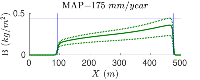
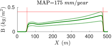
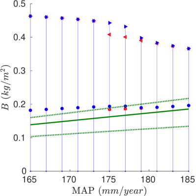
In Fig. 13 of the main text, the single-band solutions undergo a jump in terms of maximum biomass value at around 177 as precipitation is increased. Scanning down in mean annual precipitation with a single-band solution reveals a hysteresis loop associated with this jump. Figure A4 shows biomass profiles of the two distinct single-band solutions obtained at 175 . The solution found by decreasing precipitation has a lower peak biomass value, a wider vegetation band, and has a bump in biomass at the trailing edge.
The simulation results presented in the Section 5 use a fixed rain input scheme of two six-hour events spaced 6 months apart, inspired by rainfall data shown in Fig. 1. In order to explore the influence of the intensity of the rain events, we consider a fixed mean annual precipitation of 160 and vary the length of the biannual rain events. Figure A5 shows spacetime diagrams of biomass and spatial profiles for the case of 3 and 12 rainstorms.

Linear stability analysis for the coupled model, Eq. 1, shown in Fig. 3(b) indicates a drastic shrinking of the precipitation range over which the uniform state is unstable to patterns when a single 12-hour rain event per year is used instead of two equally spaced 6-hour rain events per year. Figure A6 shows that simulations of the fast-slow switching model, are consistent with these predictions. With one rain event per year, patterns are found from 89 to 147 with precipitation scans. This is a significantly narrower range than the 34 to 201 that is found with two rain events per year.
In order to explore the influence of moving towards seasonal rain input, we consider a case in which twelve rain events of 30 minutes each are evenly distributed over a rainy seasons that occurs every 6 months. Initially each rainy season spans the entire 6-month period, but the length is gradually decreased in steps of 12 every decade until the 12-event season occurs over a period of 12 days. The first row of Fig. A7 shows the initial and final patterns of instantaneous rainfall rates, from right to left. We note that, for the 12 day rainy season, there are still 12 distinct rain events of 30 minutes even though they are not resolved in the figure. For the simulation, we take the parameters given in Table 2 and a MAP of 160 . The second row shows the average biomass profiles (solid) along with the pointwise minimum and maximum (dotted) values. As the rainfall becomes more seasonal, the vegetation bands become wider with lower peak biomass value and larger fluctuations. The last two rows of Fig. A7 show the peak and averaged biomass, and the fraction of the domain covered by biomass as a function of the length of the rainy seasons. While the more seasonal rain pattern leads to a larger fraction of the domain covered by biomass, the less seasonal rain leads to more biomass on the domain. The peak biomass and average biomass values with a 12-day rainy season are approximately 0.36 and 0.79 times the corresponding values with a 6-month rainy season.
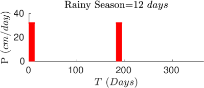
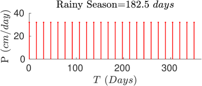
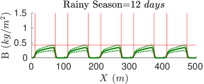
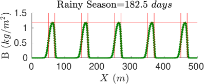


Appendix B Linear stability of the uniformly vegetated state in the three-field coupled timescale model
Here we summarize the equations used to compute the linear stability of the spatially uniform vegetation solution of the non-dimensionalized version of the three-field coupled timescale model (6), in the case of temporally periodic precipitation , where is the (minimal) period associated with the rain events. The uniform solution satisfies the following system of ordinary differential equations:
| (10) | |||||
where, recall,
| (11) |
The linear variational equations, associated with a perturbation of the form are obtained by inserting the ansatz
into the coupled model (6) and linearizing in . The resulting linear ordinary differential equations, with time-periodic coefficients, are
Here the -periodic Jacobian matrix , associated with (B), is
where is short-hand for , etc. The zero subscripts emphasize that the infiltration function , Eq. 11, is to be evaluated on the spatially uniform solution.
The Floquet multipliers, for a given perturbation wavenumber and a given periodic precipitation function , are obtained as the eigenvalues of the Monodromy matrix . In practice, to compute , we must first determine a good approximation of the initial condition for the -periodic solution . Since this solution is stable to perturbations with we can obtain an excellent approximation to the initial condition by forward-time integration of the ordinary differential equations (B). Once we have the initial condition we simultaneously solve (B) with the linearized equations (B) over one period for three independent initial conditions . The resulting form the columns of the Monodromy matrix . If all the eigenvalues of are inside the unit circle then the uniform -periodic solution is stable to perturbations of wavenumber . (Our approach to computing the Floquet multipliers associated with Eq. (B) follows that described in the textbook [J.D. Meiss, Differentiable Dynamical Systems. SIAM, 2017].)