Simulation and Optimization of Mean First Passage Time Problems in 2-D using Numerical Embedded Methods and Perturbation Theory

Abstract

We develop novel numerical methods and perturbation approaches to determine the mean first passage time (MFPT) for a Brownian particle to be captured by either small stationary or mobile traps inside a bounded 2-D confining domain. Of particular interest is to identify optimal arrangements of small absorbing traps that minimize the average MFPT. Although the MFPT, and the associated optimal trap arrangement problem, has been well-studied for disk-shaped domains, there are very few analytical or numerical results available for general star-shaped domains or for thin domains with large aspect ratio. Analytical progress is challenging owing to the need to determine the Neumann Green’s function for the Laplacian, while the numerical challenge results from a lack of easy-to-use and fast numerical tools for first computing the MFPT and then optimizing over a class of trap configurations. In this direction, and for the stationary trap problem, we develop a simple embedded numerical method, based on the Closest Point Method (CPM), to perform MFPT simulations on elliptical and star-shaped domains. For periodic mobile trap problems, we develop a robust CPM method to compute the average MFPT. Optimal trap arrangements are identified numerically through either a refined discrete sampling approach or from a particle-swarm optimization procedure. To confirm some of the numerical findings, novel perturbation approaches are developed to approximate the average MFPT and identify optimal trap configurations for a class of near-disk confining domains or for an arbitrary thin domain of large aspect ratio.

65M06, 65N06, 35C20, 35K05, 35J05

1 Introduction

The concept of first passage time has been successfully employed in studying problems in several fields of physical and biological sciences such as physics, biology, biochemistry, ecology, and biophysics, among others (see [5], [6], [9] [19], [17], and the references therein). The mean first passage time (MFPT) is defined as the average timescale for which a stochastic event occurs [21]. Some interesting problems formulated as MFPT or narrow escape problems include calculating the time it takes for a predator to locate its prey [9], the time required for diffusing surface-bound molecules to reach a localized signaling region on a cell membrane [3], and the time needed for proteins searching for binding sites on DNA [14], among others. In this paper, we are interested in the time it take for a Brownian particle to be captured by small absorbing traps in a bounded 2-D domain. Narrow escape or MFPT problems have been studied extensively both numerically and analytically using techniques such as the method of matched asymptotic expansions, and there is a growing literature on this topic (see [15], [2], [8], [10], [20], [16], [3], and [9], and the references therein).

There are two main classifications of MFPT problems in this context: one where the absorbing traps are stationary [3], [9], [2], and the other where the traps are mobile [10], [20]. For the situation with stationary traps, the MFPT can be calculated analytically and explicitly for a one-dimensional domain, and for a disk-shaped domain with a circular trap located at the center of the disk. For domains with multiple traps where the trap radius is relatively small compared to the length-scale of the domain, the method of matched asymptotic expansions can be used to derive an approximation for the MFPT (see [2], [8], [10], [20], [16]). This method can also be used to approximate the MFPT in a regular one- or two-dimensional domain with a moving trap [15], [20], [10]. However, in the case of an irregular domain, computing the MFPT has proven to be challenging both analytically and numerically. The main difficulty in solving this problem analytically arises from determining the corresponding Green’s function in the noncircular confining domain, while the challenges in the numerical computation arises from implementing the appropriate boundary conditions, especially for the case of a moving trap, where the location of the trap changes over time. Tackling such a problem numerically requires a technique that continuously updates the location of the trap, while enforcing the necessary boundary conditions at each time-step. Some commercial finite element software packages have been employed in studying MFPT problems of this form [20]. However, for other complicated MFPT problems such as determining the optimal configuration of a prescribed number of traps that minimizes the average MFPT under a continuous deformation of the boundary of the domain, the use of standard software packages is both tedious and challenging since the user has little control of the software.

In this paper, we develop a closest point method (CPM) to numerically compute the mean first passage time for a Brownian particle to escape a 2-D bounded domain for both stationary and mobile traps. CPMs are embedded numerical techniques that use e.g., finite differences to discretize partial differential equations (PDEs) and interpolation to impose boundary conditions or other geometric constraints [18, 11, 13, 12]. In addition to computing the MFPT, we will explore some interesting optimization experiments that focus on minimizing the average capture time of a Brownian particle with respect to both the location of small traps in the domain and the geometry of irregular 2-D domains.

More specifically, we will use the CPM to compute the average MFPT for a Brownian particle in both an elliptical domain and a class of star-shaped domains that contains small stationary traps. One primary focus is to use the CPM together with a particle swarm optimization procedure [7] so as to numerically identify trap configurations that minimize the average MFPT in 2-D domains of a fixed area whose boundary undergoes a continuous deformation starting from the unit disk. In particular, we will show numerically that an optimal ring pattern of three traps in the unit disk, as established in [8], deforms into a colinear arrangement of traps for a long thin ellipse of the same area. For stationary traps, novel perturbation approaches will be developed to approximate the optimal average MFPT in near-disk domains and for long-thin domains of high aspect ratio. Moreover, certain optimal closed trajectories of a moving trap in a circular or elliptical domain are identified numerically from our CPM approach. In the limit of large rotation frequency analytical results for the optimal trajectory of a moving trap are presented to confirm our numerical findings.

In the remainder of this introduction we introduce the relevant PDEs for the MFPT and average MFPT in 2-D domains with stationary and mobile traps. A brief outline of the paper is given at the end of this introductory material.

1.1 Derivation of the MFPT model

Consider a Brownian particle on a 1-D interval $[0,L]$ that makes a discrete jump of size $\Delta x$ within a small time interval $\Delta t$. Suppose that this particle can exit the interval only through the end points at $x=0$ and $x=L$. Let $u(x)$ be the MFPT for the particle to exit the interval starting from a point $x\in[0,L]$. Then, $u(x)$ can be written in terms of the MFPT at the two neighboring points of $x$ by $u(x)=\frac{1}{2}\left[u(x-\Delta x)+u(x+\Delta x)\right]+\Delta t$. The absorbing end points imply the boundary conditions $u(0)=0$ and $u(L)=0$: the particle escapes immediately if it starts at a boundary point. By Taylor-expanding and taking the limits $\Delta x\to 0$ and $\Delta t\to 0$ such that $D=(\Delta x)^{2}/\Delta t$, the discrete equation reduces to the ODE problem

$$D\,u_{xx}=-1\,,\quad 0<x<L\,;\qquad u(0)=0\,,\quad u(L)=0\,,$$

where $D$ is the diffusion coefficient of the particle. This derivation can be readily adopted to a scenario where the ends of the interval $[0,L]$ are reflecting but the interval contains a stationary absorbing trap of length $2\varepsilon$, with $\varepsilon>0$, centered at the point $x_{*}\in[0,L]$. In this case, the end points have no-flux boundary conditions, while zero-Dirichlet boundary conditions are specified on the boundaries of the trap. Consequently, the MFPT $u(x)$ for the Brownian particle satisfies

$$\begin{gathered}D\,u_{xx}=-1\,,\quad x\in(0,x_{*}-\varepsilon)\,\cup\,(x_{*}+\varepsilon,L)\,;\\ u_{x}(0)=u_{x}(L)=0\,;\quad u(x_{*}-\varepsilon)=u(x_{*}+\varepsilon)=0\,.\end{gathered}$$

Next, we derive the MFPT problem for a moving trap. This derivation is slightly different from that of a stationary trap because it requires tracking the location of the moving trap at each time-step. We start by considering a particle performing a 1-D random walk on the interval $[0,L]$, which contains a small mobile absorbing trap that moves in a periodic path contained in the interval. Similar to above, the discrete equation for the MFPT $u(x,t)$ satisfies

$$u(x,t)=\frac{1}{2}\left[u(x-\Delta x,t+\Delta t)+u(x+\Delta x,t+\Delta t)\right]+\Delta t\,.$$

Upon Taylor expanding in $\Delta x$ and $\Delta t$, and taking the limits $\Delta x\to 0$ and $\Delta t\to 0$, such that $D=(\Delta x)^{2}/(2\Delta t)$, the resulting PDE for the MFPT $u(x,t)$ is

$$\begin{gathered}u_{t}+Du_{xx}+1=0,\quad x\in(0,x_{*}(t)-\varepsilon)\,\cup\,(x_{*}(t)+\varepsilon,L),\;\;0<t<T,\\ u(x,0)=u(x,T),\,\,u(x_{*}(t)-\varepsilon,t)=0,\,\,u(x_{*}(t)+\varepsilon,t)=0,\,\,u_{x}(0,t)=u_{x}(L,t)=0,\end{gathered}$$

where $T$ is the period of oscillation of the trap. Due to the oscillations of the trap, we have imposed the time-periodic boundary condition $u\left(x,0\right)=u\left(x,T\right)$, which specifies that the MFPT at each point in the domain should be the same after each period. The conditions $u(x_{*}(t)-\varepsilon,t)=0$ and $u(x_{*}(t)+\varepsilon,t)=0$ imply that the particle is captured by the edges of the moving trap. Finally, we impose the no-flux conditions $u_{x}(0,t)=u_{x}(L,t)=0$ to ensure that the outer boundaries are reflecting.

1.2 MFPT problems in 2-D

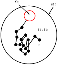
For an arbitrary bounded domain $\Omega\subset\mathbb{R}^{2}$, containing $m$ small stationary absorbing traps $\Omega_{1},\dots,\Omega_{m}$ (such as shown in Figure 1 for $m=1$), the MFPT $u(\mathbf{x})$ for a Brownian particle starting at a point $\mathbf{x}\in\bar{\Omega}$ is

(1) $$\begin{split}D\,\nabla^{2}u=-1\,,&\quad\mathbf{x}\in\bar{\Omega}\,;\\ \partial_{n}u=0\,,\,\,\,\mathbf{x}\in\partial\Omega\,;&\qquad u=0\,,\,\,\,\mathbf{x}\in\partial\Omega_{i}\,,\qquad i=1,\dots,m\,,\end{split}$$

where $\mathbf{x}\equiv(x,y)$, $D$ is the diffusion coefficient of the particle, $\partial_{n}$ denotes the outward normal derivative on the domain boundary $\partial\Omega$, and $\bar{\Omega}=\Omega\setminus\cup_{i=1}^{m}\Omega_{i}$.

(a)      (b)

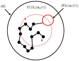
Figure 1: Brownian particles in disk-shaped regions with absorbing traps. In (a), a particle starting at $\mathbf{x}\in\Omega\setminus\Omega_{0}$ in $\Omega$ eventually hits a stationary absorbing trap $\Omega_{0}$. In (b), the trap $\Omega_{0}(\mathbf{x}_{0}(t))$ rotates about the center of the region.

If the traps are moving in periodic paths with positions $\mathbf{x}_{i}(t)$ (see Figure 1), then the corresponding MFPT problem is

(2) $$\begin{split}&u_{t}+D\nabla^{2}u+1=0\,,\quad\mathbf{x}\in\bar{\Omega}(t)\,;\\ &\partial_{n}u=0\,,\,\,\mathbf{x}\in\partial\Omega\,;\qquad u=0\,,\,\,\mathbf{x}\in\partial\Omega_{i}(t)\,;\qquad u(\mathbf{x},0)=u(\mathbf{x},T)\,,\end{split}$$

where $T$ is the period of the moving traps. Often it will be useful to write the periodic motion in terms of an angular frequency $\omega$, where $T={2\pi/\omega}$.

1.2.1 Time reversal

Our numerical calculations will work significantly better if we solve problem (2) “backwards” in time, e.g., after the change of variables $\tau=-t$. The problem is still periodic in $\tau$ with periodic $T$, namely

(3) $$\begin{split}&u_{\tau}=D\nabla^{2}u+1\,,\quad\mathbf{x}\in\Omega\setminus\bar{\Omega}(\tau)\,;\\ &\partial_{n}u=0\,,\,\,\mathbf{x}\in\partial\Omega\,;\qquad u=0\,,\,\,\mathbf{x}\in\partial\Omega_{i}(\tau)\,;\qquad u(\mathbf{x},0)=u(\mathbf{x},T)\,.\end{split}$$

1.3 An elliptic problem

Suppose that the domain $\Omega\subset\mathbb{R}^{2}$ is a disk containing a single moving trap centered at $\mathbf{x}_{0}(t)$ that rotates about the center of the disk on a ring in the clockwise direction, such as illustrated in Figure 1. In this case, using the change of variables $(x,y)=(r\cos\theta,r\sin\theta)$, with $0<r\leq 1$, and $0\leq\theta\leq 2\pi$, (2) can be written in polar coordinates, with the trap center given by $\mathbf{x}_{0}(t)=(r_{0}\cos(\omega t),r_{0}\sin(\omega t))$, where $r_{0}$ is the distance from the center of the trap to the center of the disk. Furthermore, setting $\phi=\theta-\textrm{mod}(\omega t,2\pi)$ with $0<\phi<2\pi$, and $u(r,\theta,t)=u(r,\phi(t))$, the MFPT problem reduces to the elliptic PDE problem

(4) $$\begin{split}D\,\nabla^{2}u+\omega u_{\phi}+1=0\,,&\quad\mathbf{x}\in\Omega\setminus\Omega_{0}(r_{0})\,;\\ u=0\,,\,\,\,\mathbf{x}\in\partial\Omega_{0}(r_{0})\,;\quad&\partial_{n}u=0\,,\,\,\,\mathbf{x}\in\partial\Omega\,.\end{split}$$

Here $\nabla^{2}u$ is the Laplacian in polar coordinates, and $u_{\phi}$ is the derivative of $u$ in the transformed angular coordinate (see [10], [20] for more details). This reformulation enables us to study an elliptic PDE, as compared to a more challenging time-dependent parabolic problem. However, (4) can only be employed in studying MFPT problems in a domain that is invariant with respect to the location of the moving trap.

1.4 Feature extraction

The MFPT depends on the starting location $\mathbf{x}$ of the particle. Assuming a uniform distribution of starting locations, the average/expected MFPT for a particle to exit the region starting from anywhere in the domain is

(5) $$\begin{split}\overline{u}=\frac{1}{|\bar{\Omega}|}\int_{\bar{\Omega}}u(\mathbf{x})\,\text{d}\mathbf{x}\,,\qquad\mbox{where }\quad|\bar{\Omega}|=|\Omega\backslash\cup_{i=1}^{m}\Omega_{i}|\,,\end{split}$$

and $|\bar{\Omega}|$ denotes the area of $\bar{\Omega}$. For the case of a moving trap, the average MFPT is

(6) $$\begin{split}\overline{u}=\frac{1}{T\,|\bar{\Omega}|}\int_{0}^{T}\int_{\bar{\Omega}}u(\mathbf{x},t)\,\,\,\text{d}\mathbf{x}\,\text{d}t\,.\end{split}$$

The time integral averages the MFPT over a period, which ensures that the escape time of the particle is independent of the location of the trap. These average MFPT quantities will be used below in our computation and optimization experiments.

In § 2, we discuss numerical techniques to compute solutions to our MFPT problems. In § 3 and § 4, we give numerical results for some MFPT problems with stationary traps and a moving trap, respectively. Moreover, some numerical optimization experiments are performed to identify trap configurations that minimize the average MFPT for a Brownian particle. In § 5, asymptotic results for the MFPT, based on various perturbation schemes, are used to confirm some of our numerical results in § 3 and § 4. A brief discussion in § 6 concludes the paper.

2 The numerical algorithm

Closest Point Methods (CPMs) are numerical techniques for solving PDEs on curved surfaces and other irregularly shaped domains. The key idea is to embed the physical domain of interest into an unfitted numerical grid enveloping the surface. All grid points that lie on the interior of the domain are simply physical solution values, while those that lie outside the domain are used to impose boundary conditions. In this paper, we apply the closest point method to mean first passage time problem in 2-D domains. Solving MFPT problems numerically in 2-D domains using regular finite difference methods comes with certain difficulties. Most notably, implementing boundary conditions on curved boundaries is complicated because grid points do not lie on those curves. Fitted grids (such as triangulations) can approximate curved boundaries but require frequent remeshing in moving boundary problems. Embedded methods avoid these remeshing steps.

2.1 Closest points

Every grid point is associated with its closest point (by Euclidean distance) in the physical domain $\textrm{cp}(\mathbf{x}):=\textrm{argmin}_{\mathbf{y}\in\bar{\Omega}}\|\mathbf{x}-\mathbf{y}\|_{2}$, where we recall that the domain of our PDE is $\bar{\Omega}=\Omega\setminus\cup_{i=1}^{m}\Omega_{i}$. Note if $\mathbf{x}$ is an interior point, its closest point is simply itself: $\textrm{cp}(\mathbf{x})=\mathbf{x}$. The closest point function can be precomputed in closed form for simple shapes, for example, for a disc of radius $R$ punctured by a small $\varepsilon$-radius hole, such a function could be given by

$$\textrm{cp}_{\textrm{punc.disc}}(\mathbf{x})=\begin{cases}(\varepsilon,0)&\text{if $\mathbf{x}=(0,0)$,}\\ \varepsilon\frac{\mathbf{x}}{\|\mathbf{x}\|}&\text{if $\|\mathbf{x}\|<\varepsilon$,}\\ \mathbf{x}&\text{if $\varepsilon\leq\|\mathbf{x}\|\leq R$,}\\ R\frac{\mathbf{x}}{\|\mathbf{x}\|}&\text{otherwise (i.e., $\|\mathbf{x}\|>R$).}\end{cases}$$

We assume that we have either approximate or exact samples of the closest-point function available for our method; this is our preferred representation of the geometry.

The cp function can be used to extend functions defined in the domain out into the ambient space surrounding the domain. The simplest such extension is

(7) $$v(\mathbf{x}):=u(\textrm{cp}(\mathbf{x})),$$

which defines a function $v:B(\bar{\Omega})\to\mathbb{R}$ which agrees with $u:\bar{\Omega}\to\mathbb{R}$ for points $\mathbf{x}\in\bar{\Omega}$ and is constant in the normal direction outside of the domain $\bar{\Omega}$. Here $B(\bar{\Omega})\supset\bar{\Omega}$, for example all of $\mathbb{R}^{2}$ or a padded bounding box of $\bar{\Omega}$. In practice, we only need $B(\bar{\Omega})$ to be only a few grid points larger than $\bar{\Omega}$ itself.

2.2 Imposing boundary conditions using extensions

Suppose we want to impose a homogeneous Neumann boundary condition $\partial_{n}u=0$ at all points along some curve $\gamma$ making up all or part of the boundary of $\bar{\Omega}$. Given $u:\bar{\Omega}\to\mathbb{R}$, we construct $v(\mathbf{x}):=u(\textrm{cp}(\mathbf{x}))$ to obtain a function $v$ which is constant in the normal direction, and thus satisfies the homogeneous Neumann boundary condition. A spatial differential operator applied to $v$ will then respect the zero-Neumann condition automatically.

For a more general Neumann boundary condition, $\partial_{n}u=g_{1}(\mathbf{x})$ for $\mathbf{x}\in\gamma$, we (formally) perform a finite difference in the normal direction to obtain $\frac{u(\mathbf{x})-u(\textrm{cp}(\mathbf{x}))}{\|\mathbf{x}-\textrm{cp}(\mathbf{x})\|_{2}}\approx u_{n}(\textrm{cp}(\mathbf{x}))=g_{1}(\textrm{cp}(\mathbf{x})).$ Rearranging to solve for $u(\mathbf{x})$ we define the extension:

$$v(\mathbf{x}):=u(\textrm{cp}(\mathbf{x}))+\|\mathbf{x}-\textrm{cp}(\mathbf{x})\|_{2}\,g_{1}(\textrm{cp}(\mathbf{x})),$$

Note as $\mathbf{x}\to\textrm{cp}(\mathbf{x})$, we have $v(\mathbf{x})\to u(\textrm{cp}(\mathbf{x}))$ so $u$ is continuous at the boundary. However, the extended solution is not very smooth (it may have a corner at $\gamma$) and this leads to a loss of numerical accuracy [11]. Indeed the above formula was constructed using first-order finite differences; we can improve the formal order of accuracy to at least two by using a centered difference [11].

2.2.1 Second-order accurate boundary extensions: Neumann

We construct a “mirror point” $\overline{\textrm{cp}}(\mathbf{x}):=\mathbf{x}+2(\textrm{cp}(\mathbf{x})-\mathbf{x})=2\textrm{cp}(\mathbf{x})-\mathbf{x}$ which consists of a point reflected across the boundary $\gamma$ [11]. As above, we then apply centered differences around the point $\textrm{cp}(\mathbf{x})$ and solve for $u(\mathbf{x})$, in order to define

$$v(\mathbf{x}):=u(\overline{\textrm{cp}}(\mathbf{x}))+\|\mathbf{x}-\overline{\textrm{cp}}(\mathbf{x})\|_{2}\,g_{1}(\textrm{cp}(\mathbf{x})).$$

Again we see continuity as $\mathbf{x}\to\textrm{cp}(\mathbf{x})$ but now we can expect the extension to be smoother because instead of just $u(\textrm{cp}(\mathbf{x}))$ we now have information about how $u(\overline{\textrm{cp}}(\mathbf{x}))\to u(\textrm{cp}(\mathbf{x}))$ is included.

2.2.2 Dirichlet boundary extensions

The general Dirichlet boundary condition, that $u(\mathbf{x})=g_{2}(\mathbf{x})$ for some specified function $g_{2}$, can be implemented by copying the value of $g_{2}$ for points outside the domain using $v(\mathbf{x}):=g_{2}(\textrm{cp}(\mathbf{x}))$, but as before this is a low-accuracy approximation due to lack of smoothness. A more accurate extension comes from specifying that the average value matches the given data $\frac{1}{2}\big{(}v(\mathbf{x})+u(\overline{\textrm{cp}}(\mathbf{x})\big{)}=g_{2}(\textrm{cp}(\mathbf{x}))$ from which we define

$$v(\mathbf{x}):=2g_{2}(\textrm{cp}(\mathbf{x}))-u(\overline{\textrm{cp}}(\mathbf{x})),$$

which differs from the Neumann case primarily by a change of sign in front of $u(\overline{\textrm{cp}}(\mathbf{x}))$.

2.2.3 Combinations of boundary conditions

Combining these various extensions we define an operator $E$ which extends solutions by

(8a) $$v:=Eu+g\,,$$

where operator $$E g$$ and functional are the homogeneous and non-homogeneous parts of the extensions respectively:

(8b) $$v(\mathbf{x}):=\begin{cases}u(\mathbf{x})&\mathbf{x}\in\bar{\Omega}\\ u(\overline{\textrm{cp}}(\mathbf{x})&\textrm{cp}(\mathbf{x})\in\gamma_{\textrm{n}}\\ -u(\overline{\textrm{cp}}(\mathbf{x})&\textrm{cp}(\mathbf{x})\in\gamma_{\textrm{d}}\end{cases}+\begin{cases}0&\mathbf{x}\in\bar{\Omega},\\ \|\mathbf{x}-\overline{\textrm{cp}}(\mathbf{x})\|_{2}\,g_{1}(\textrm{cp}(\mathbf{x}))&\textrm{cp}(\mathbf{x})\in\gamma_{\textrm{n}},\\ 2g_{2}(\textrm{cp}(\mathbf{x}))&\textrm{cp}(\mathbf{x})\in\gamma_{\textrm{d}},\end{cases}$$

where $\gamma_{\textrm{n}}$ and $\gamma_{\textrm{d}}$ indicate boundaries with Neumann and Dirichlet conditions respectively. Although not needed here, all of the above constructions can also be applied on curved surfaces embedded in $\mathbb{R}^{3}$ or higher and of arbitrary codimension [11].

2.2.4 Discretizations of extensions

Although some of the above extensions were motivated by finite differences, they are not discrete because $\textrm{cp}(\mathbf{x})$ and $\overline{\textrm{cp}}(\mathbf{x})$ are not generally grid points (due to the curved boundary $\gamma$). One way to discretize is to use a polynomial interpolation scheme to approximate $u(\overline{\textrm{cp}}(\mathbf{x}))$ using a stencil of grid points neighboring $\overline{\textrm{cp}}(x)$. The typical choice is a $4\times 4$ grid which allows bicubic interpolation [18]. Equivalently, we can use the sample values of $u$ at those same 16 points to build a bicubic polynomial which approximates $u$; we then compute the exact extension of that polynomial.

Some of these stencils will contain points outside of $\bar{\Omega}$. This is not a problem because all functions will be defined over $B(\bar{\Omega})$. That is, we do not really have $u$ and $v$, only $v:B(\bar{\Omega})\to\mathbb{R}$. What is crucial however is that all discrete stencils lie inside $B(\bar{\Omega})$; this is how we define the computational domain: the set of all grid points $\mathbf{x}$ such that the stencil around $\overline{\textrm{cp}}(\mathbf{x})$ is contained in the set [13].

2.3 Imposing boundary conditions with a penalty

We wish to spatially discretize the PDE (3) using finite differences and standard time-stepping schemes. A systematic procedure is needed to ensure that $v$ remains an appropriate extension so that such a computation respects the boundary conditions. The approach of [22] modifies the problem by introducing a penalty for change that does not satisfy the extension. Ignoring the time-periodic condition $u(\mathbf{x},0)=u(\mathbf{x},T)$ for the moment, the idea is that we want to solve

(9a) $$v_{t} =D\nabla^{2}v+1,\qquad\mathbf{x}\in\bar{\Omega},$$

subject to the constraint that

(9b) $$v =Ev+g,\qquad\mathbf{x}\in B(\bar{\Omega}),\,\,\mbox{and for all relevant $t$.}$$

This system can be achieved by extending the right-hand side of (9a), introducing a parameter $\bar{\gamma}$, and combining the two equations [22] to give

(10) $$v_{t} =\bar{E}D\nabla^{2}v+1-\bar{\gamma}(v-Ev-g),\quad\mathbf{x}\in B(\bar{\Omega}),\,\,\,\text{and for all relevant $t$,}$$

where $\bar{E}$ is the closest point extension (7).

2.3.1 Method of lines discretization

The extension operators can be discretized into matrices by collecting the coefficients of the polynomial interpolant, e.g., using Barycentric Lagrange Interpolation [13]. This allows us to write (8) as

$$\mathbf{v}:=\mathbf{E}_{h}\mathbf{u}+\mathbf{g}\,,$$

where $\mathbf{v}$ is a long vector of the pointwise samples of the function $v$ at the grid points in the computational domain. We use a uniform grid of $B(\bar{\Omega})$ with grid spacing $h=\Delta x$. The Laplacian operator is replaced by a square matrix $\mathbf{L}_{h}$ where each row consists of $\left\{\tfrac{1}{h^{2}\rule{0.0pt}{3.91806pt}},\tfrac{1}{h^{2}\rule{0.0pt}{3.91806pt}},\tfrac{-4}{h^{2}\rule{0.0pt}{3.91806pt}},\tfrac{1}{h^{2}\rule{0.0pt}{3.91806pt}},\tfrac{1}{h^{2}\rule{0.0pt}{3.91806pt}}\right\}$ and many zeros. Combining these spatial operators, we then discretize (10) using the method of lines to obtain an ODE system

(11) $$\mathbf{v}_{t} =\bar{\mathbf{E}}_{h}D\mathbf{L}_{h}\mathbf{v}+\mathbf{1}-\frac{4D}{h^{2}}\Big{(}\mathbf{v}-\mathbf{E}_{h}\mathbf{v}-\mathbf{g}\Big{)}\,,\qquad\text{for all relevant $t$\,,}$$

where we have used $\bar{\gamma}=\frac{2\text{dim}}{h^{2}}D$ as recommended by [22]. We can then apply forward Euler, backward Euler or some other time-stepping scheme to (11) using discrete time-step size of $\Delta t$. For example, backward Euler would be

(12) $$\frac{\mathbf{v}^{n+1}-\mathbf{v}^{n}}{\Delta t} =\left[D\bar{\mathbf{E}}_{h}\mathbf{L}_{h}-\frac{4D}{h^{2}}\Big{(}\mathbf{I}-\mathbf{E}_{h}\Big{)}\right]\mathbf{v}^{n+1}+\frac{4D}{h^{2}}\mathbf{g}+\mathbf{1}\,,$$

where $\mathbf{v}^{n}$ is a vector of the approximate solution at each grid point at time $t=n\Delta t$.

2.3.2 Elliptic solves

The elliptic problem (4) can be discretized in a similar way [1] using the penalty approach. We obtain the discretization

(13a) $$D\bar{\mathbf{E}}_{h}\mathbf{L}_{h}\mathbf{v}-\frac{4D}{h^{2}}\Big{(}\mathbf{v}-\mathbf{E}_{h}\mathbf{v}-\mathbf{g}\Big{)}+\Big{(}\mathbf{S}_{1}\mathbf{D}_{h}^{x}\mathbf{v}+\mathbf{S}_{2}\mathbf{D}_{h}^{y}\mathbf{v}\Big{)}+\mathbf{1}=\mathbf{0}\,,$$

where $$\mathbf{D}_{h}^{x} \mathbf{D}_{h}^{y} \left\{-\tfrac{1}{2h},0,\tfrac{1}{2h}\right\} \mathbf{S}_{1} \mathbf{S}_{2} s_{1}(x,y) s_{2}(x,y)$$ and are centered differences using weights , and and are diagonal matrices with the local advection vector coefficients and , extended by (7), on the diagonal. For our specific problem (4), we have

(13b) $$s_{1}(x,y)=\omega r\cos\theta,\,\,s_{2}(x,y)=-\omega r\sin\theta,\,\,\mbox{where}\,\,r^{2}=x^{2}+y^{2},\,\theta=\tan^{-1}\!\left(\tfrac{y}{x}\right).$$

If $\omega$ is large, upwinding differences should be used for the advection.

2.4 Relaxation to a time-periodic solution

In our moving trap problem (3), the traps $\Omega_{i}(\mathbf{x}_{i}(t))$ are moving, and thus the domain $\bar{\Omega}$ is changing over time. This means the discretization operators $\mathbf{E}_{h}$ and $\bar{\mathbf{E}_{h}}$ are changing at each time step. At least in principle the grid itself could also change although for simplicity of implementation we include all grid points in the interior of the small traps (even if not strictly needed). We assume that the traps do not move too far per timestep—not more than one or two grid points—to avoid large discretization errors.

In our moving domain problems, the period $T={2\pi/\omega}$ of the motion is known and we look for solutions which satisfy the time-periodic boundary condition $u(\mathbf{x},0)=u(\mathbf{x},T)$. An “all-at-once” discretization of both space and time simultaneously could be prohibitive in terms of memory usage. Instead, we approach this problem using a “shooting method”: we solve an initial value problem from a somewhat arbitrary initial guess at $t=0$ for many periods. Due to the dissipative nature of the PDE, we expect this procedure to converge to a time-periodic solution.

2.4.1 Stopping criterion

At the end of the $N$th period we compare the numerical solution at $t=NT$ with that from $t=(N-1)T$. We define a tolerance tol and stop the calculation when $\|\mathbf{v}(NT)-\mathbf{v}((N-1)T)\|\leq\texttt{tol}$, in some norm; typically we use the change in the average MFPT as our stopping criterion.

2.5 Feature extraction

Visualizing the solution can be accomplished by coloring all grid points according to the numerical solution value, with grid points outside the physical domain simply omitted. We also need to extract features of the solution, such as the maximum value, or the average over space and time from § 1.4. Spatial integrals of the solution can be extracted using quadrature although care must be taken near the edges of the domain to ensure second-order accuracy. We use a modified quadrature weight [4] to integrate the numerical solution over a non-rectangular domain. Temporal integration is done using Trapezoidal Rule.

3 Numerical computations for stationary trap problems

In this section, the CPM is used to compute solutions for some MFPT problems in 2-D domains with stationary traps. Moreover, some stationary trap configurations that optimize the average MFPT are identified numerically.

3.1 MFPT for a concentric stationary trap in a disk

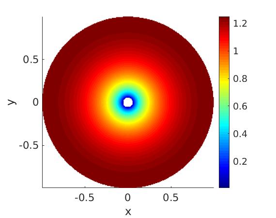
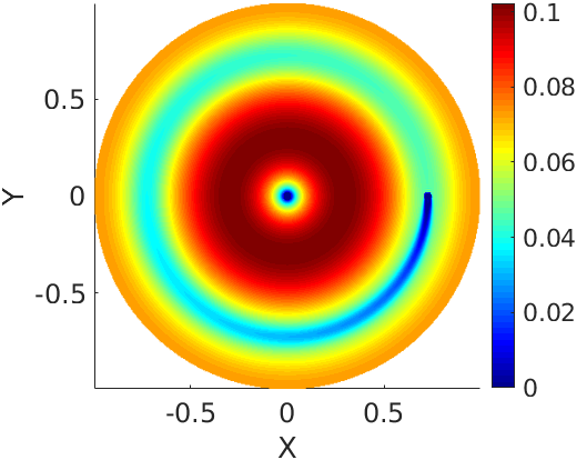
We use the CPM to compute the MFPT for a Brownian particle in the unit disk with a concentric stationary trap of radius $\varepsilon=0.05$. The result is shown in Figure 2. Based on the figure colormap we observe the intuitive result that the MFPT is smaller for particles that start closer to the trap than for those that start farther away.

3.2 Convergence Study

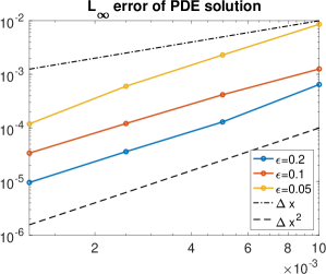
We use the exact solution $u(r)=\frac{1}{4}(\varepsilon^{2}-r^{2})+\frac{1}{2}\log(r/\varepsilon)$ for the MFPT to perform a convergence study of our numerical method. For several values of the trap radius $\varepsilon$, and various grid spacings $\Delta x$, we numerically compute the MFPT. The resulting $L_{\infty}$ error is shown in Figure 2. As $\varepsilon$ decreases, the exact solution has a stronger gradient owing to the logarithmic term. This leads to a poorer convergence of the numerical solution. Nevertheless, we observe second-order convergence of the numerical solution as $\Delta x\to 0$, as expected from § 2.2.1.

(a)   (b)

Figure 2: Convergence studies on the punctured unit disk for various values of the trap radius $\varepsilon$, confirming second-order convergence of our elliptic solver. (a) MFPT, with colormap indicating the time for capture starting at $\mathbf{x}$. (b) $L_{\infty}$ error versus $\Delta x$.

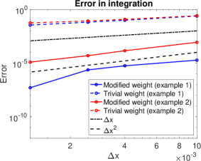
Next, we study the accuracy of the numerical quadrature $I_{h}=\sum_{i,j}\omega_{i,j}u^{h}_{i,j}$ of the numerical solution $u^{h}$ on rectangular grid. The trivial weight $\omega_{i,j}=1$ is only first order accurate. We compare it with second-order accurate modified weight [4] by computing the area of the perforated domains shown in Figure 3. The convergence study in Figure 3, shows that the convergence rate using the trivial weight is only first order, with an error significantly larger than the mesh size $\Delta x$. However, by using the modified weight for numerical integration, we observe a second-order convergence rate in both examples.

(a) (b) (c)

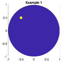
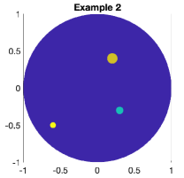
Figure 3: Two examples of the unit disk perforated by circular traps. (a) one trap centered at $\mathbf{x}_{1}=(-0.5,0.5)$ with radius $\varepsilon_{1}=0.05$. (b) three traps centered at $\mathbf{x}_{1}=(0.3,-0.3)$, $\mathbf{x}_{2}=(0.2,0.4)$, and $\mathbf{x}_{3}=(-0.6,-0.5)$, with radii $\varepsilon_{1}=0.05,\,\varepsilon_{2}=0.07$, and $\varepsilon_{3}=0.04$, respectively. (c) accuracy of the numerical integration to compute the trap-free areas for (a) and (b), using trivial and modified weights.

Having confirmed the numerical accuracy and convergence of the CPM, we now consider more intricate problems where analytic solutions are not available. In certain cases, the novel asymptotic approaches developed later in § 5 are used to compare with our computational results.

3.3 MFPT in a disk with traps arranged on a ring

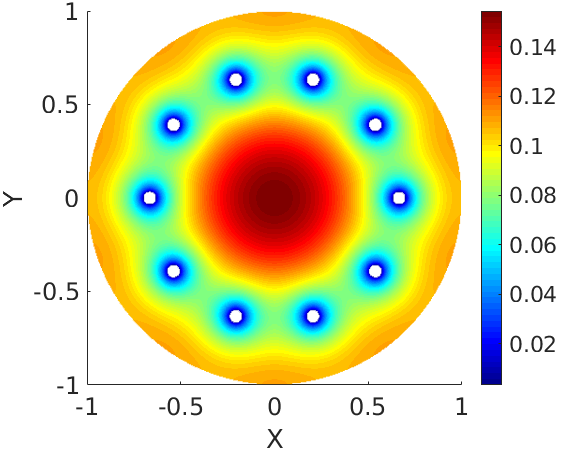
We consider a pattern of $m\geq 2$ circular traps that are equally-spaced on a ring of radius $0<r<1$, concentric within the unit disk. In [8] it was shown using asymptotic analysis that for each $m\geq 2$ there is a unique ring radius $r_{c}$ that minimizes the average MFPT for this pattern. We now validate this result numerically. To do so, we solve (1) for a given $m$ with many different possible radii $r$. The numerically optimal ring radius $r_{c}$ is taken as the value of $r$ for which the average MFPT is minimized. Specifically, we discretized the ring radius $r$ with a resolution of $\Delta r=0.0001$. For each discrete value of $r$, we solved for the average MFPT using the CPM with numerical grid spacing $\Delta x=0.004$. We then took $r_{c}$ as the minimum value over the resulting discrete set.

(a) MFPT for the optimal 10 trap ring.

$m$	Asymptotics	Numerics
2	0.4536	0.4533
3	0.5517	0.5480
4	0.5985	0.5987
5	0.6251	0.6275
6	0.6417	0.6411
7	0.6527	0.6467
8	0.6604	0.6609
9	0.6662	0.6689
10	0.6706	0.6708

(b) Optimal ring radius $r_{c}$ for $m$ traps.

Figure 4: The optimal ring radius $r_{c}$ for $m$ circular traps of radius $\varepsilon=3\times 10^{-3}$ that are equally-spaced on a ring concentric within a reflecting unit disk. For each $m\geq 2$, the optimal radius $r_{c}$ minimizes the average MFPT for such a ring pattern of traps. (a) Optimal MFPT computed from the CPM with $m=10$. (b) Comparison of our numerical results with the asymptotic results obtained in [8].

Figure 4(a) shows the MFPT for $m=10$ traps on a ring with the optimal radius $r_{c}=0.6708$ computed by the procedure above. The table in Figure 4(b) shows a close comparison of our numerical results with the asymptotic results obtained in [8].

3.4 Two stationary traps in an elliptical domain

Next, we consider the MFPT for a family of elliptical domains with semi-minor axis $b$, with $b<1$, and semi-major axis $a={1/b}>1$ that contains two circular absorbing traps of radius $\varepsilon$ centered on the major axis. As $b$ is decreased from unity, an initial circular domain gradually deforms into an elliptical region of increasing eccentricity, with the area of the domain fixed at $\pi$. As $b$ is varied, we will compute the optimal location of the traps that minimize the average MFPT. For each fixed $b<1$, the centers of the two traps are varied on the major axis with a step size of $0.01$, and for each such configuration the average MFPT is computed. The optimal trap locations at the given $b$ correspond to where the average MFPT is smallest. The computations were done with a numerical grid spacing of $\Delta x=0.005$, and the semi-minor axis was decreased in steps of $\Delta b=0.02$. Our numerical simulation predicts, as expected, that the optimal locations of the two traps must be symmetric about the minor axis. For the unit disk where $b=1$, our numerical results yield that the optimal locations of the traps is at a distance $x_{0}=0.450$ from the center of the disk. This agrees with computations in § 3.3 (see Figure 4(b)) of a two-trap ring pattern in a unit disk.

(a) MFPT for optimal traps

(b) Optimal location of traps

(c) Optimal average MFPT

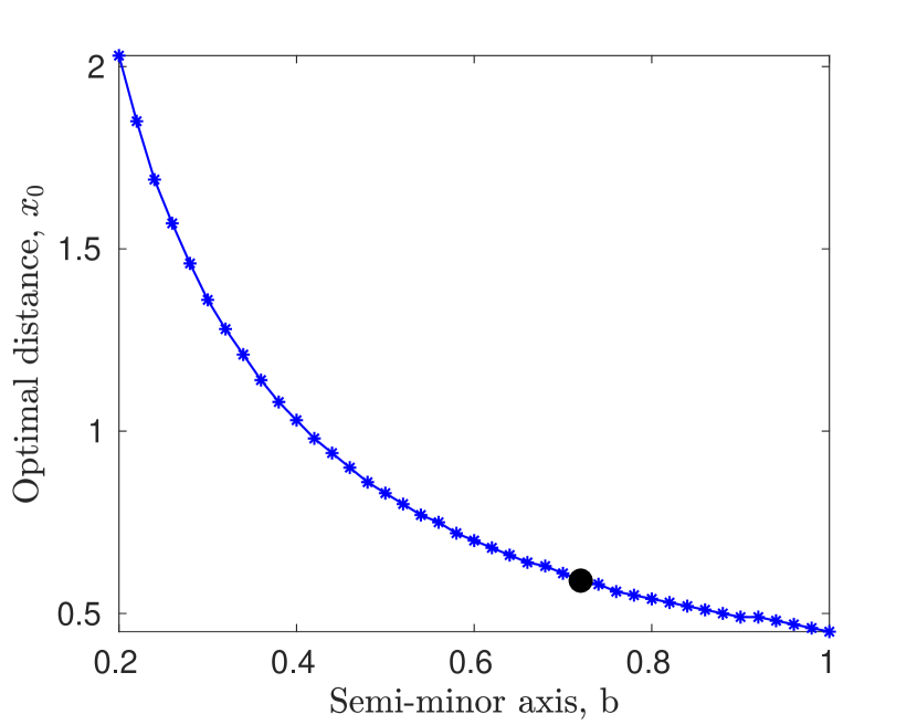
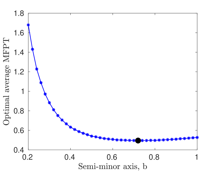
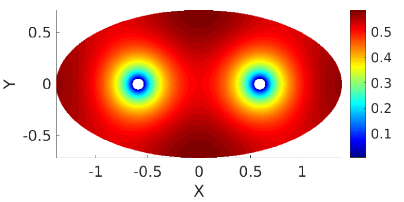
Figure 5: Two traps of radii $\varepsilon=0.05$ on the major axis of an elliptical domain. Left: with semi-major axis $a\approx 1.3889$ and semi-minor axis $b=1/a=0.72$, the optimal location for the traps are $(\pm 0.59,0)$. Middle: the optimal trap locations change as we shrink the minor axis. Right: the average MFPT for optimal trap locations as the semi-minor axis is varied. The dot is the globally minimal average MFPT $\overline{u}_{\textrm{opt}}=0.4954$, over all ellipses of area $\pi$; it occurs in the configuration shown in (a).

Figure 5(a) shows the MFPT for an elliptical region of semi-major axis $a=1.3889$ and semi-minor axis $b=0.72$, with two circular traps of radius $\varepsilon=0.05$ on its major axis centered at $(\pm 0.59,0)$. These are the optimal locations of the traps for this particular elliptical region. Figures 5(b) and 5(c) show the optimal locations of the traps and the optimal average MFPT, respectively, as the semi-minor axis, $b$, is decreased. We observe from this figure that the optimal traps move away from each other as $b$ decreases. This is because, as the eccentricity of the ellipse increases, narrow regions at the two ends of the major axis are created in which a Brownian particle can “hide” from the traps. This effective “pinning” of particles by the domain geometry increases their escape time. In order to reduce the escape time of such pinned particles—and thus the overall average MFPT for the region—the traps need to move closer to the ends of the major axis.

Figure 5(c) shows that as $b$ is decreased the optimal average MFPT initially decreases until a global minimum $\overline{u}_{\textrm{opt}}=0.4954$ is reached at $b\approx 0.72$. This corresponds to traps that are at a distance $x_{0}=0.59$ from the center of the ellipse (see Figure 5(a) for the MFPT of this pattern). This result suggests that the geometry that gives the global minimum MFPT for the two-trap pattern is an elliptical region with semi-major axis $a=1.3889$ and semi-minor axis $b=0.72$, and most notably is not the unit disk. In § 5.1 we perform an asymptotic analysis to determine the optimal MFPT and trap locations in near-disk domains, which verifies that the global minimum of the MFPT is not attained by the unit disk but rather for a specific elliptical domain. Moreover, in § 5.2 an asymptotic approach based on thin domains is used to predict the optimal trap locations and optimal average MFPT when $b\ll 1$.

3.5 Three stationary traps in an ellipse

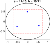
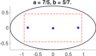
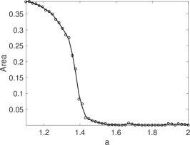
From [8] a ring pattern of three equally-spaced traps provides the optimal three-trap configuration to minimize the average MFPT in the unit disk. However, it is more intricate to determine the optimal three-trap pattern in an elliptical domain. To do so numerically, we employ the Matlab built-in function particleswarm for particle swarming optimization (PSO) [7], to compute a local minimum of the MFPT for an elliptical domain $\frac{x^{2}}{a^{2}}+\frac{y^{2}}{b^{2}}=1$ with $a=1.1$ and $b={10/11}$. This optimal configuration is shown in the left panel of Figure 6. We use this optimization result to initialize the numerical computation of local minima of MFPT with the Matlab built-in function fmincon for other values of $a$. For $1.1\leq a\leq 2$, and fixing the area of the ellipse at $\pi$, in the right panel of Figure 6 we plot the area of the triangle formed by the numerically optimized locations of the three traps. This figure shows that the three traps becomes colinear as $a$ is increased. In § 5.2.2, an asymptotic analysis, tailored for long thin domains, is used to predict the optimal locations of these three colinear traps for $a\gg 1$.

Figure 6: The CPM and PSO is used to numerically compute local minimizers of the MFPT for three trap patterns in a one-parameter family of ellipses $(\frac{x}{a})^{2}+(\frac{y}{b})^{2}=1$ with trap radius $\varepsilon=0.05$, $1.1\leq a\leq 2$ and $b={1/a}$. The right panel is for the area of the triangle formed by the three traps, which shows that the optimal traps become colinear as $a$ increases. The red dashed rectangles show the bounds used for PSO.

3.6 Traps in star-shaped domains

We briefly investigate the MFPT for multiple static traps in a star-shaped domain, defined as the region bounded by

(14) $$r=1+\sigma\cos(\mathcal{N}\theta)\,,\quad 0<\theta<2\pi\,,\quad 0<\sigma<1\,,$$

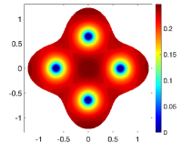
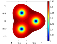
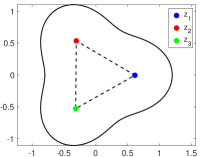
where $(r,\theta)$ are polar coordinates. Here $\mathcal{N}$ is a positive integer that determines the number of folds in the domain boundary. We use the CPM together with particle swarm optimization [7] to numerically compute a local minimizer of the MFPT for two specific examples. In Figure 7 we show the optimal MFPT and trap locations for a three-trap pattern in a three-fold star-shaped domain ($\mathcal{N}=3$) and for a four-trap pattern in a four-fold star-shaped domain ($\mathcal{N}=4$). In our asymptotic analysis of the optimal MFPT in near-disk domains in § 5.1 we will predict the optimal trap locations when $m=\mathcal{N}$ and $\sigma\ll 1$. For $\sigma\ll 1$, we will show that the optimal trap locations are aligned on rays where the boundary deflection is at a maximum.

Figure 7: Numerically computed optimal $\mathcal{N}$-trap patterns in $\mathcal{N}$-fold star-shaped domains, found by PSO. Left two: PDE solution and optimal locations for $\mathcal{N}=3$; the optimal locations form an equilateral triangle on the circle of radius approximately $0.615$, to within a numerical error of $0.005$. Right two: $\mathcal{N}=4$; the square has vertices on the circle of radius approximately $0.65$. Here $\sigma=0.2$ and trap radii are $\varepsilon=0.05$.

4 Numerical computation for moving trap problems

In this section, we will consider several problems for a Brownian particle in a domain with moving traps.

4.1 Convergence study

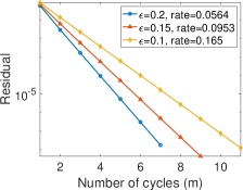
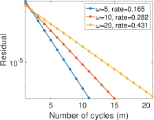
We first study the rate of convergence of our time relaxation approach discussed in § 2.4. Consider the unit disk with a trap moving in a circular path concentric within the disk at a fixed radius $r_{0}=0.6$ from the origin. At period $N$ of the algorithm, using the notation in § 2.4.1, we compute residual $\|\mathbf{v}(NT)-\mathbf{v}((N-1)T)\|_{L_{2}}$. We study the rate of convergence of the residual under different choices of mesh size $\Delta x$, the radius of the trap $\varepsilon$, and the rotation speed $\omega$. In Figure 8 we show that the number of cycles for convergence is of $\mathcal{O}(1)$ and, in particular, is independent of the mesh size $\Delta x$. This figure shows that the key factors that determine the rate of convergence are the trap radius $\varepsilon$ and the angular frequency $\omega$ of the circular trajectory of the trap. We use Forward Euler timestepping in these numerical convergence studies.

(a) (b) (c)

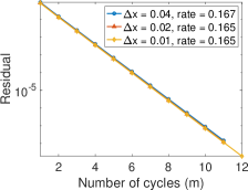
Figure 8: Convergence studies for our time relaxation strategy for a trap moving on a ring of radius $r_{0}=0.6$ within the unit disk. In (a) we fix the trap radius $\varepsilon=0.1$ and angular frequency $\omega=5$, and vary the mesh size with $\Delta x=0.04,0.02$ and $0.01$; the rate of convergence is almost independent of the mesh size. In (b) we fix the angular frequency $\omega=5$ and mesh size $\Delta=0.02$, and test three choices of trap radius $\varepsilon=0.2,0.15$ and $0.1$; smaller trap radii lead to slower convergence. In (c) we fix the trap radius $\varepsilon=0.1$ and mesh size $\Delta x=0.02$, and consider three angular frequencies $\omega=5,10$ and $20$; larger angular frequencies lead to slower convergence.

4.2 Optimizing the radius of rotation of a moving trap in a disk

Consider an absorbing circular trap of radius $\varepsilon=0.05$ that rotates on a ring of radius $r$ about the center of a reflecting unit disk at a constant angular frequency $\omega$, as illustrated in Figure 1. For any fixed $\omega$ and $r$ value, we can compute the MFPT using our time relaxation strategy with mesh size $\Delta x=0.01$, and forward Euler time-stepping with $\Delta t={\Delta x/f(\omega)}$, where $f(\omega)$ is a linear functions of the angular frequency $\omega$. The iteration proceeds over many cycles until the tolerance from § 4.1 is satisfied. A typical result is shown, at a fixed instant in time, in Figure 9.

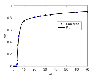
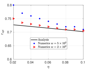
To estimate numerically the radius $r_{\textrm{opt}}(\omega)$ of rotation of the trap that minimizes the average MFPT as a function of $\omega$, we choose a discrete set of $\omega$ values and for each such value estimate $r_{\textrm{opt}}$ by computing the average MFPT for different discrete radii of rotation of the trap. We then record the $r$ value that gives the minimum average MFPT as $r_{\textrm{opt}}$. In choosing the discrete radii set, various values of $\Delta r$ were used, depending on $\omega$. The results are shown in Figure 9. The use of discrete sets of $r$ values induces some mild stair-casing artifacts into the plot. In Figure 9 (and elsewhere), we have added a heuristic fit to the data points.

(a)    (b)

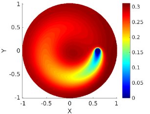
Figure 9: Left: the MFPT at a given time for a circular trap of radius $\varepsilon=0.05$ rotating at an angular frequency of $\omega=100$ about the center of a unit disk on a ring of radius $r=0.6$. Right: the optimal radius of rotation $r_{\textrm{opt}}(\omega)$ that minimizes the average MFPT at a given rotation frequency $\omega$.

From Figure 9 we observe that there is a critical rotation frequency $\omega_{b}$, estimated numerically as $\omega_{b}\approx 3.131$, where the optimal radius of rotation changes from a zero to a positive value. When $\omega<\omega_{b}$, the location of the trap that minimizes the average MFPT is at the center of the unit disk. Alternatively, when $\omega>\omega_{b}$, the optimal trap moves away from the center of the domain. This problem has previously been studied analytically in [20] using asymptotic analysis valid in the limit of small trap radius. In [20], the critical value of $\omega_{b}$ was calculated asymptotically as $\omega_{b}\approx 3.026$, which is close to what we obtained numerically.

4.3 Optimizing the trajectory of a trap in an elliptical region

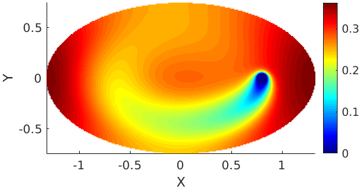
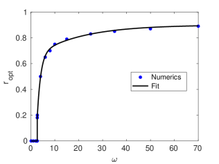
Next, we consider a circular absorbing circular trap of radius $\varepsilon=0.05$ that is rotating at constant angular frequency on an elliptical orbit about the center of an elliptical region as shown in Figure 10. The elliptical path for the trap is taken as $(x,y)=(\alpha\cos(\omega t),\beta\sin(\omega t)$, where $\alpha=ra$, $\beta=rb$, and $a$ and $b$ are the semi-major and semi-minor axis of the elliptical region, respectively. We choose $a=4/3$ and $b={1/a}=3/4$, so that the area of the ellipse is the same as that for the unit disk. The parameter $0<r<(1-\varepsilon)$, referred to as the radius of rotation, is used to stretch or shrink the orbit of the trap. This parameterization ensures that the eccentricity of all elliptical paths of the trap is the same as that of the domain boundary.

Similar to that done in § 4.2, for various angular frequencies $\omega$ we numerically determine the optimal radius of rotation $r_{\textrm{opt}}(\omega)$ that minimizes the average MFPT. The results are shown in Figure 10. As similar to the case of the unit disk, we observe for the elliptical domain that there is a critical value of $\omega$ where the optimal radius bifurcates from the origin. We estimate this numerically as $\omega_{b}\approx 2.65$.

(a)    (b)

Figure 10: The MFPT for a moving trap of radius $\varepsilon=0.05$ in an ellipse. The trap rotates on an elliptical path with semi-major axis $\alpha=ra$ and semi-minor axis $\beta=rb$ in an elliptical region with semi-major axis $a=4/3$ and semi-minor axis $b=3/4$. (a) MFPT at an instant in time with $\omega=100$ and $r=0.6$. (b) The optimal radius $r_{\textrm{opt}}(\omega)$ which minimizes the average MFPT for each $\omega$.

4.4 Optimizing one rotating trap and one fixed trap in a disk

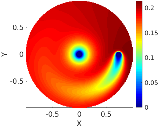
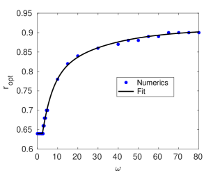
Next, we consider the unit disk in which there are two circular absorbing traps each of radius $\varepsilon=0.05$. One of the traps is fixed at the center of the disk while the other one is rotating at constant angular frequency $\omega$ about the center of the disk on a ring of radius $r$ concentric within the disk.

(a)    (b)

Figure 11: The average MFPT for a unit disk with a trap at the center and a trap rotating with angular frequency $\omega$ around the center at radius $r$. The traps have radii $\varepsilon=0.05$. (a) MFPT at an instant in time with $r=0.6$ and $\omega=100$. (b) The optimal radius $r_{\textrm{opt}}(\omega)$ for the moving trap, which minimizes the average MFPT for each $\omega$. These values were found using a discrete search with $\Delta r=0.01$.

As a function of $\omega$, we proceed similarly to § 4.2 to estimate numerically the radius of rotation of the moving trap that minimizes the average MFPT. The results for the optimal radius are shown in Figure 11. From this figure, we observe that there is a specific angular frequency $\omega_{b}$, estimated as $\omega_{b}\approx 2.5$, at which the optimal radius first begins to increase from the fixed value $r_{\textrm{opt}}=0.64$ when $\omega$ increases beyond $\omega_{b}$. This critical frequency is lower than that computed in § 4.2 for a single rotating trap in the unit disk. An analysis to predict the optimal radius in the fast rotation limit $\omega\gg 1$ for this problem is given in § 5.3.

5 Analysis

In this section, we provide some new analytical results to confirm some of our numerical findings. First, in § 5.1 we use strong localized perturbation theory (cf. [23], [24]), to confirm some of our predictions on the optimum locations of steady traps in perturbed disk-shaped domains. Next, in § 5.2 we use a novel singular perturbation approach to estimate optimal locations of colinear traps in long thin domains. Finally, in § 5.3, we develop an analytical approach to study the moving trap problem in a disk in the limit of fast rotation. For these three problems we will focus on summarizing our main analytical results: a detailed derivation of them is given in the Supplementary Material.

5.1 Asymptotic analysis of the MFPT for a perturbed unit disk

We begin by calculating the MFPT for a slightly perturbed unit disk that contains $m$ traps. In the unit disk, and for small values of $m$, the optimal trap configuration consists of equally-spaced traps on a ring concentric within the disk [8]. When the disk is perturbed into a star-shaped domain with $\mathcal{N}$ folds, we will develop an asymptotic method to determine how the optimal trap locations and optimal average MFPT associated with the unit disk are perturbed. For the special case where $m=\mathcal{N}$ explicit results for these quantities are derived. The results from this analysis are used to confirm some of the numerical results in § 3.4 and § 3.6.

For $\sigma\ll 1$, we use polar coordinates to define the perturbed unit disk as

(15) $$\Omega_{\sigma}=\Big{\{}(r,\theta)\,\Big{|}\,0<r\leq 1+\sigma\cos(\mathcal{N}\theta),\,\,0\leq\theta\leq 2\pi\Big{\}}.$$

Observe that $\Omega_{\sigma}$ is a star-shaped domain with $\mathcal{N}$ folds for any $\sigma>0$, and it tends to the unit disk, denoted by $\Omega$, as $\sigma\to 0$. From (1) the MFPT for a Brownian particle starting at a point $\mathbf{x}\in\bar{\Omega}_{\sigma}$ to be absorbed by a trap satisfies

(16) $$\begin{split}D\,\nabla^{2}u=-1,&\quad\mathbf{x}\in\bar{\Omega}_{\sigma};\\ \partial_{n}u=0,\quad\mathbf{x}\in\partial\Omega_{\sigma};&\qquad u=0,\quad\mathbf{x}\in\partial\Omega_{\varepsilon j},\quad j=0,\dots,m-1,\end{split}$$

where $\bar{\Omega}_{\sigma}\equiv\Omega_{\sigma}\setminus\cup_{j=1}^{m}\Omega_{\varepsilon j}$ is the perturbed domain with the trap set deleted, while $\Omega_{\varepsilon j}=\{\mathbf{x}:|\mathbf{x}-\mathbf{x}_{j}|\leq\varepsilon\}$ is the $j^{\text{th}}$ absorbing trap centered at $\mathbf{x}_{j}=r_{c}\exp\big{(}i(2\pi j/m+\psi)\big{)}$ with $\psi>0$, for $j=0,\dots,m-1$ on the ring of radius $r_{c}$. A simple calculation shows that the area of the star-shaped domain is $|\Omega_{\sigma}|=|\Omega|+{\mathcal{O}}(\sigma^{2})$. Our goal is to use perturbation methods to reduce the MFPT problem for the perturbed disk (16) to problems involving the unit disk. Using the parameterization $\mathbf{x}\equiv(x,y)=(r\cos(\theta),r\sin(\theta))$, the Neumann boundary condition in (16) can be written as

(17) $$\begin{split}u_{r}-&\frac{\sigma h_{\theta}}{(1+\sigma h)^{2}}u_{\theta}=0\quad\text{on}\quad r=1+\sigma h,\quad\text{where}\quad h(\theta)=\cos(\mathcal{N}\theta).\end{split}$$

We begin by expanding the MFPT $u$ in terms of $\sigma\ll 1$ as

(18) $$\begin{split}u(r,\theta;\sigma)=u_{0}(r,\theta)+\sigma u_{1}(r,\theta)+\sigma^{2}u_{2}(r,\theta)+\ldots.\end{split}$$

Upon substituting (18) into (16) and (17), and collecting terms in powers of $\sigma$, we derive that the leading-order MFPT problem satisfies

(19) $$\begin{split}D\,\nabla^{2}u_{0}=-1,&\quad\mathbf{x}\in\bar{\Omega};\\ \partial_{n}u_{0}=0,\quad\text{on}\quad r=1;&\qquad u_{0}=0,\quad\mathbf{x}\in\partial\Omega_{\varepsilon j},\qquad j=0,\dots,m-1,\end{split}$$

where $\bar{\Omega}\equiv\Omega\setminus\cup_{j=1}^{m}\Omega_{\varepsilon j}$. At next order, the $\mathcal{O}(\sigma)$ problem is

(20) $$\begin{split}\nabla^{2}u_{1}=0,&\quad\mathbf{x}\in\bar{\Omega};\qquad\partial_{r}u_{1}=-hu_{0rr}+h_{\theta}u_{0\theta},\quad\text{on}\quad r=1;\\ \quad u_{1}&=0,\quad\mathbf{x}\in\partial\Omega_{\varepsilon j},\qquad j=0,\dots,m-1,\end{split}$$

with $h\equiv h(\theta)$ as given in (17). We emphasize that the leading-order problem (19) and the $\mathcal{O}(\sigma)$ problem (20), are formulated on the unit disk and not on the perturbed disk. Assuming $\varepsilon^{2}\ll\sigma$, we use (5) and $|\Omega_{\sigma}|=|\Omega|+{\mathcal{O}}(\sigma^{2})$ to derive an expansion for the average MFPT for the perturbed disk in terms of the unit disk as

(21) $$\begin{split}\overline{u}=\frac{1}{|\Omega|}\!\int_{\Omega}\!u_{0}(\mathbf{x})\,\text{d}\mathbf{x}+\sigma\!\left[\frac{1}{|\Omega|}\!\int_{\Omega}\!u_{1}(\mathbf{x})\,\text{d}\mathbf{x}+\frac{1}{|\Omega|}\!\int_{0}^{2\pi}\!h(\theta)\,u_{0}|_{r=1}\,\text{d}\theta\right]+\mathcal{O}(\sigma^{2},\varepsilon^{2}),\end{split}$$

where $|\Omega|=\pi$, $h(\theta)=\cos(\mathcal{N}\theta)$, and $u_{0}|_{r=1}$ is the leading-order solution $u_{0}$ evaluated on $r=1$. In the Supplementary Material we show how to calculate $u_{0}$ and $u_{1}$, which then yields $\overline{u}$ from (21). This leads to the following main result:

Proposition 1.

Consider a near-disk domain with boundary $r=1+\sigma\cos(\mathcal{N}\theta)$, with $\sigma\ll 1$, that has $m$ traps equally-spaced on a ring of radius $r_{c}$, centered at $\mathbf{x}_{j}=r_{c}e^{i\theta_{j}}$, where $\theta_{j}={2\pi j/m}+\psi$ for $j=0,\ldots,m-1$. Then, if ${\mathcal{N}/m}\in\mathbb{Z}^{+}$, where $\mathbb{Z}^{+}$ is the set of positive integers, we have in terms of the ring radius $r_{c}$ and the phase shift $\psi$ that the average MFPT satisfies

(22a) $$\overline{u}\sim\overline{u}_{0}+\sigma\overline{U}_{1}+\ldots\,,$$

(22b) $$\overline{u}_{0}=\frac{1}{2m\nu D}+\frac{\pi\kappa_{1}}{mD},\;\;\overline{U}_{1}=-\frac{r_{c}^{\mathcal{N}}}{\mathcal{N}D}\cos(\mathcal{N}\psi)\!\left(\frac{2+(\mathcal{N}-2)r_{c}^{2m}}{1-r_{c}^{2m}}-\frac{\mathcal{N}}{2}(k-1)\!\right)\!,$$

(22c) $$\mbox{and}\quad\kappa_{1}=\frac{1}{2\pi}\left[-\log(mr_{c}^{m-1})-\log(1-r_{c}^{2m})+mr_{c}^{2}-\frac{3}{4}m\right],$$

where $$k\equiv{\mathcal{N}/m} k\in\mathbb{Z}^{+} {\mathcal{N}/n}\notin\mathbb{Z}^{+} \overline{u}\sim\overline{u}_{0}+{\mathcal{O}}(\sigma^{2})$$ and . Alternatively, if , then .

This result shows that there are two distinct cases: ${\mathcal{N}/m}\in\mathbb{Z}^{+}$ and ${\mathcal{N}/m}\notin\mathbb{Z}^{+}$. In the latter case, the correction to the average MFPT at ${\mathcal{O}}(\sigma)$ vanishes, and a higher-order asymptotic theory would be needed to determine the correction term at ${\mathcal{O}}(\sigma^{2})$. We do not pursue this here.

In the analysis below we will focus on the case where $\mathcal{N}=m$ and will use our result in (22) to optimize the average MFPT with respect to the radius $r_{c}$ of the ring and the phase shift $\psi$. We observe from (22b) that $\overline{u}$ is minimized when $\psi=0$. Therefore, the optimal traps on the ring are on rays from the origin that coincide with the maxima of the boundary perturbation given by $\max(1+\sigma\cos(\mathcal{N}\theta))\equiv 1+\sigma$. To optimize $\overline{u}$ with respect to $r_{c}$, we write $\overline{u}_{0}=\overline{u}_{0}(r_{c})$ and $\overline{U}_{1}=\overline{U}_{1}(r_{c})$ and expand

(23) $$r_{c\,\textrm{opt}}=r_{c_{0}}+\sigma\,r_{c_{1}}+\ldots\,.$$

Here $r_{c_{0}}$ is the leading-order optimal ring-radius obtained by setting $\overline{u}_{0}^{\prime}(r_{c})=0$ in (22b). In this way, for any $m\geq 2$, we obtain $r_{c_{0}}$ is the unique root on $0<r_{c_{0}}<1$ to

(24) $$\frac{r_{c}^{2m}}{(1-r_{c}^{2m})}=\frac{m-1}{2m}-r_{c}^{2}.$$

Numerical values for this root for various $m$ were given in the table in Figure 4.

Next, we substitute (23) into the expansion in (22a), and collect terms in powers of $\sigma$. In this way, the optimal average MFPT is given by

(25) $$\begin{split}\overline{u}_{\textrm{opt}}&\sim\overline{u}_{0}(r_{c_{0}})+\sigma\overline{U}_{1}(r_{c_{0}})+\ldots,\end{split}$$

where $\overline{u}_{0}$ and $\overline{U}_{1}$ are as defined in (22b). Moreover, by setting $\overline{u}^{\prime}(r_{c})=0$ and expanding $r_{c}$ as in (23), we obtain that $r_{c_{1}}=-{\overline{U}_{1}^{\prime}(r_{c_{0}})/\overline{u}_{0}^{\prime\prime}(r_{c_{0}})}$. This yields that

(26) $$r_{c_{1}}=\frac{1}{\pi}\frac{\chi^{\prime}(r_{c_{0}})}{\kappa_{1}^{\prime\prime}(r_{c_{0}})}\,;\quad\chi^{\prime}(r_{c_{0}})=-\frac{mr_{c_{0}}^{m-1}}{(1-r_{c_{0}}^{2m})^{2}}\Big{[}(m-2)r_{c_{0}}^{4m}+(4-3m)r_{c_{0}}^{2m}-2\Big{]},$$

and $\kappa_{1}^{\prime\prime}(r_{c_{0}})$ is the second derivative of $\kappa_{1}(r_{c})$ as defined in (22c), evaluated at the leading-order optimal radius $r_{c_{0}}$. Since $r_{c_{0}}$ is a minimum point of $\kappa_{1}(r_{c})$, then $\kappa_{1}^{\prime\prime}(r_{c_{0}})>0$. Also, it can easily be shown that $\chi^{\prime}(r_{c_{0}})>0$ for $0<r_{c_{0}}<1$. Thus, $r_{c_{1}}>0$, which implies that the centers of the traps bulge outwards towards the maxima of the domain boundary perturbation. This result is summarized as follows:

Proposition 2.

In the near disk case with boundary $r=1+\sigma\cos(\mathcal{N}\theta)$ and $\sigma\ll 1$, and for a ring pattern with $m=\mathcal{N}$ traps equally spaced on a ring of radius $r_{c}$, the optimal radius $r_{c\,\textrm{opt}}$ of the ring is given by

(27a) $$r_{c\,\textrm{opt}}\sim r_{c_{0}}+\,\frac{\sigma}{\pi}\frac{\chi^{\prime}(r_{c_{0}})}{\kappa_{1}^{\prime\prime}(r_{c_{0}})}+\ldots\,,$$

(27b) $$\text{where}\qquad\kappa_{1}^{\prime\prime}(r_{c_{0}})=\frac{m}{\pi r_{c_{0}}^{2}}\left[\frac{(m-1)}{2m}+r_{c_{0}}^{2}+\frac{r_{c_{0}}^{2m}}{(1-r_{c_{0}}^{2m})^{2}}\Big{(}2m-1+r_{c_{0}}^{2m}\Big{)}\right]\,.$$

Here $\chi^{\prime}(r_{c_{0}})$ is given in (26) in terms of the unique solution $r_{c_{0}}$ to (24).

We first apply our results to an ellipse of area $\pi$ that contains two circular traps each of radius $\varepsilon=0.05$ centered on the major axis. This corresponds to the early stage of deformation of the unit disk in the optimal MFPT problem studied in § 3.4 (see Figure 5). The boundary of the ellipse is parameterized for $\sigma\ll 1$ by $(x,y)=(a\cos(\theta)\,,b\sin(\theta))$, for $0\leq\theta<2\pi$, where $a=1+\sigma$ and $b=1/(1+\sigma)$ are the semi-axes chosen so that $ab=1$ for any $\sigma>0$. For $\sigma\ll 1$, we readily calculate that the domain boundary in polar coordinates is $r=1+\sigma\cos(2\theta)+{\mathcal{O}}(\sigma^{2})$.

Upon setting $m=2$ and $\mathcal{N}=2$ in (27), and then using $\sigma=(b^{-1}-1)$ as $b\to 1^{-}$, we obtain that the optimal ring radius satisfies

(28a) $$r_{c\,\textrm{opt}}\sim r_{c_{0}}+\frac{1}{\pi}\left(\frac{1}{b}-1\right)\,\frac{\chi^{\prime}(r_{c_{0}})}{\kappa_{1}^{\prime\prime}(r_{c_{0}})},$$

where $$r_{c_{0}}\approx 0.4536 m=2 m=2$$ is the unique root of (24) when . Here, from (27b) and (26) with , we have that

(28b) $$\chi^{\prime}(r_{c_{0}})=\frac{4r_{c_{0}}(r_{c_{0}}^{4}+1)}{(1-r_{c_{0}}^{4})^{2}}\,,\quad\mbox{and}\quad\kappa_{1}^{\prime\prime}(r_{c_{0}})=\frac{2}{\pi\,r_{c_{0}}^{2}}\left[\frac{1}{4}+r_{c_{0}}^{2}+\frac{r_{c_{0}}^{4}(3+r_{c_{0}}^{4})}{(1-r_{c_{0}}^{4})^{2}}\right].$$

By setting $r_{c_{0}}=0.4536$ in (28), (25), and (22) we obtain for a trap radius of $\varepsilon=0.05$ that the optimal ring radius and the optimal average MFPT are

(29) $$r_{c\,\textrm{opt}}(b)\sim 0.4536+\left(\tfrac{1}{b}-1\right)0.3559,\quad\overline{u}_{\textrm{opt}}\sim\frac{1}{D}\Big{[}0.5120-\left(\tfrac{1}{b}-1\right)0.2149\Big{]},$$

as $b\to 1^{-}$. This perturbation result characterizes the optimal trap locations and optimal average MFPT for a slight elliptical perturbation of the unit disk.

(a) Optimal location of traps

(b) Optimal average MFPT

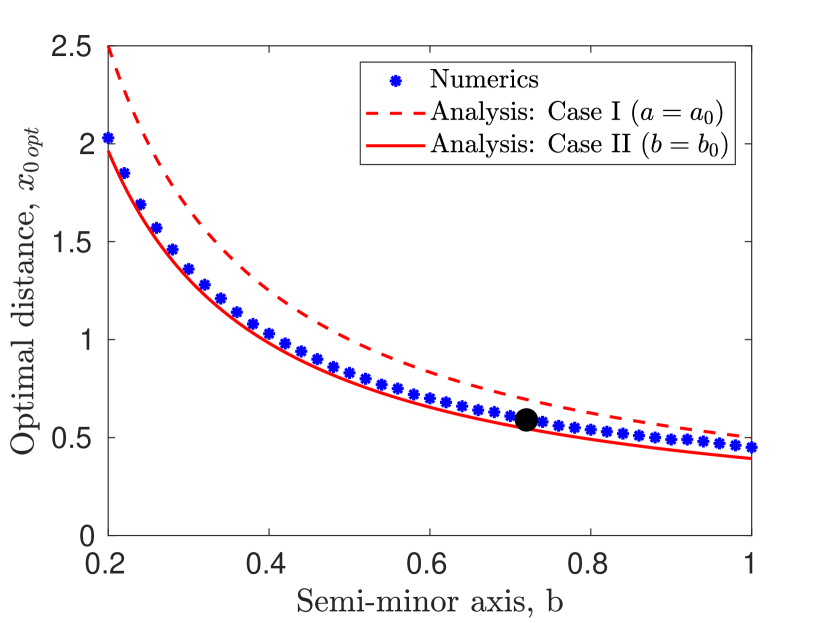
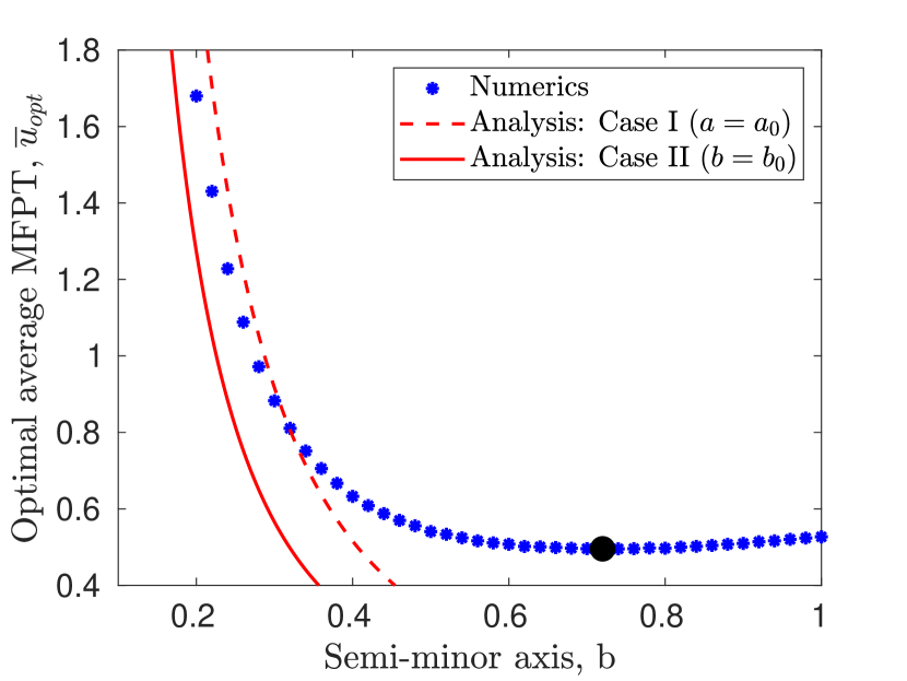
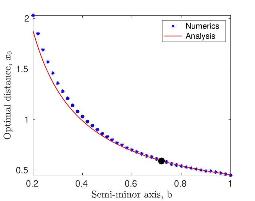
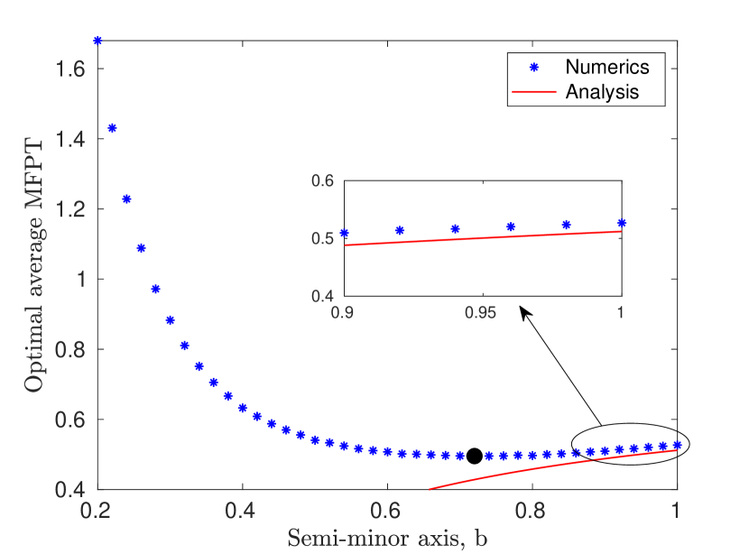
Figure 12: Two traps in an ellipse: a comparison of the perturbation results in (29) (thin lines) with the full numerical results (asterisks) of Figure 5 for the deforming elliptical region containing two traps of radius $\varepsilon=0.05$. The asymptotic theory is valid for semi-minor axis $b\to 1^{-}$ (early stages of disk deformation). (a) optimal distance of the traps from the center of the ellipse versus $b$. (b) optimal average MFPT versus $b$. The dot is the globally optimal average MFPT found earlier in Figure 5.

For $D=1$, Figures 12(a) and 12(b) show a comparison of our analytical results (29) for the optimal location of the traps and the optimal average MFPT with the corresponding full numerical results computed using the CPM in Figure 5. Although our analysis is only valid for $b\to 1^{-}$, Figure 12(a) shows that our perturbation result for the optimal trap locations agree closely with the numerical result even for moderately small values of $b$. However, this is not the case for the optimal average MFPT, where the perturbation result deviates rather quickly from the numerical result as $b$ decreases. The key qualitative conclusion from the analysis is that the optimal average MFPT decreases as $b$ decreases below $b=1$. This establishes that, for the class of elliptical domains with fixed area $\pi$, the optimal average MFPT is minimized not for the unit disk, but for a particular ellipse.

Next, we apply our theory to the cases $m=\mathcal{N}=3$ and $m=\mathcal{N}=4$, which were studied numerically in Figure 7 when $\sigma=0.2$. For traps of radii $\varepsilon=0.05$ and $D=1$, we obtain from (27) and (25) that when $\sigma\ll 1$ the optimal ring radius and optimal average MFPT are

(30) $$r_{c,\textrm{opt}}\sim 0.5517+0.2664\,\sigma\,,\qquad\overline{u}_{\textrm{opt}}\sim 0.2964-0.1168\,\sigma\,;\qquad m=\mathcal{N}=3\,,$$

(31) $$r_{c,\textrm{opt}}\sim 0.5985+0.1985\,\sigma\,,\qquad\overline{u}_{\textrm{opt}}\sim 0.1998-0.0663\,\sigma\,;\qquad m=\mathcal{N}=4\,.$$

For $\sigma=0.2$, this yields that $r_{c,\textrm{opt}}\approx 0.6049$ when $m=\mathcal{N}=3$ and $r_{c,\textrm{opt}}\approx 0.6382$ when $m=\mathcal{N}=4$. Although $\sigma=0.2$ is not very small, the asymptotic results still provide a rather decent approximation to the numerical results for the optimal trap locations shown in Figure 7.

5.2 Asymptotics for high-eccentricity elliptical domains

In this subsection we provide two different approximation schemes for estimating the optimal average MFPT for an elliptical domain of high-eccentricity that contains either two or three traps centered along the semi-major axis.

5.2.1 Approximation by thin rectangular domains

We consider a Brownian particle in a thin elliptical domain of area $\pi$ with semi-major axis $a$ and semi-minor axis $b$, that contains two circular absorbing traps each of radius $\varepsilon$ on its major axis (see Figure 5) for $b\ll 1$. In order to estimate the MFPT for this particle, the elliptical region is replaced with a thin rectangular region defined by $[-a_{0},a_{0}]\times[-b_{0},b_{0}]$ satisfying $(a_{0}/b_{0})\gg 1$. Moreover, the circular traps in the ellipse are replaced with thin vertical trap strips of width $2\varepsilon_{0}$ centered at $(-x_{0},0)$ and $(x_{0},0)$, namely $\Omega_{1}=\Phi_{1}\times[-b_{0},b_{0}]$ and $\Omega_{2}=\Phi_{2}\times[-b_{0},b_{0}]$ where $\Phi_{1}=[-x_{0}-\varepsilon_{0}\leq x\leq-x_{0}+\varepsilon_{0}]$ and $\Phi_{2}=[x_{0}-\varepsilon_{0}\leq x\leq x_{0}+\varepsilon_{0}]$. The MFPT in this rectangular domain satisfies

(32) $$\nabla^{2}u =-1/D\,,\quad\mbox{in}\quad\mathbf{x}\in[-a_{0},a_{0}]\times[-b_{0},b_{0}]\setminus\{{\Omega_{1},\,\Omega_{2}\}}\,,$$

$$\partial_{x}u =0\,,\quad\mbox{on}\quad x=\pm a_{0}\quad\mbox{for}\quad|y|\leq b_{0}\,,$$

$$\partial_{y}u =0\,,\quad\mbox{on}\quad y=\pm b_{0}\quad\mbox{for}\quad x\in[-a_{0},a_{0}]\setminus\{{\Phi_{1},\,\Phi_{2}\}}\,,$$

$$u =0\,,\quad\text{for $x\in\Omega_{1}\cup\Omega_{2}$.}$$

To ensure that the area of the rectangular region is $\pi$ and that the rectangular traps have the same area as the circular traps in the elliptical region, we impose that

(33) $$4a_{0}\,b_{0}=\pi\quad\mbox{and}\quad 4\varepsilon_{0}\,b_{0}=\pi\,\varepsilon^{2}\,.$$

The PDE (32) has a 1-D solution that is even in $x$, namely $u_{1}(x)\equiv\frac{1}{2D}\big{(}(x_{0}-\varepsilon)^{2}-x^{2}\big{)}$ for $0\leq x\leq x_{0}-\varepsilon$, and $u_{2}(x)\equiv\frac{1}{2D}\big{[}x(2a_{0}-x)+(x_{0}+\varepsilon_{0})(x_{0}+\varepsilon_{0}-2a_{0})\big{]}$ for $x_{0}+\varepsilon\leq x\leq a_{0}$. Then, we calculate $I_{1}=\int_{0}^{x_{0}-\varepsilon}u_{1}\,\text{d}x$ and $I_{2}=\int_{x_{0}+\varepsilon}^{a_{0}}u_{2}\,\text{d}x$, and observe that the average MFPT is given by $\overline{u}=4b_{0}(I_{1}+I_{2})/\!\left(\pi(1-2\varepsilon^{2})\right)$. We get

(34) $$\overline{u}=\frac{4\,b_{0}}{D\pi(1-2\varepsilon^{2})}\Big{[}{\left(a_{0}-2\,\varepsilon_{0}\right)}x_{0}^{2}-{\left(a_{0}^{2}-2\,a_{0}\varepsilon_{0}\right)}x_{0}+\frac{1}{3}\,a_{0}^{3}-a_{0}^{2}\varepsilon_{0}+a_{0}\varepsilon_{0}^{2}-\frac{2}{3}\,\varepsilon_{0}^{3}\Big{]}.$$

The optimal locations of the traps are found by minimizing $\overline{u}$ with respect to $x_{0}$. This yields

(35) $$x_{0\,{\textrm{opt}}}=\frac{a_{0}}{2}=\frac{\pi}{8b_{0}}\,,\quad\mbox{and}\quad\overline{u}_{\textrm{opt}}=\frac{\pi^{2}}{192\,D\,b_{0}^{2}}\Big{(}1-4\,\varepsilon^{2}+\mathcal{O}(\varepsilon^{4})\Big{)}\,.$$

Here we used $a_{0}=\pi/(4\,b_{0})$ and $\varepsilon_{0}={\pi\varepsilon^{2}/(4b_{0})}$ as given in (33).

As one would expect, the optimal location in (35) is the point at which the area of the half-rectangle $[0,a_{0}]\times[-b_{0},b_{0}]$ is divided into two equal pieces. This equal area rule will minimize the capture time of the Brownian particle in the half-rectangle.

Next, we relate this optimal MFPT in the thin rectangular domain to that in the thin elliptical domain. One possibility is to set $a_{0}=a$, so that the length of the rectangular domain and the ellipse along the major axis are the same. From the equal area condition (33), we obtain $b_{0}=(\pi b)/4$, where $b$ is the semi-minor axis of the ellipse. For this choice (35) becomes

(36) $$x_{0\,{\textrm{opt}}}=\frac{1}{2b}\quad\mbox{and}\quad\overline{u}_{\textrm{opt}}\approx\frac{1}{12\,D\,b^{2}}\Big{(}1-4\,\varepsilon^{2}+\mathcal{O}(\varepsilon^{4})\Big{)}\,;\qquad\mbox{Case I:}\,\,\,(a=a_{0})\,.$$

A second possibility is to choose $b_{0}=b$, so that the width of the thin rectangle and ellipse are the same. From (35) this yields that

(37) $$x_{0\,{\textrm{opt}}}=\frac{\pi}{8b}\quad\mbox{and}\quad\overline{u}_{\textrm{opt}}\approx\frac{\pi^{2}}{192\,D\,b^{2}}\Big{(}1-4\,\varepsilon^{2}+\mathcal{O}(\varepsilon^{4})\Big{)}\,;\qquad\mbox{Case II:}\,\,\,(b=b_{0})\,.$$

Both estimates (36) and (37) are applicable only when $b\ll 1$. Together they suggest that the optimal locations of the traps and the optimal average MFPT for the thin ellipse satisfy the scaling laws $x_{0\,{\textrm{opt}}}=\mathcal{O}(b^{-1})$ and $\overline{u}_{\textrm{opt}}=\mathcal{O}(b^{-2})$, respectively.

(a) Optimal location of traps

(b) Optimal average MFPT

Figure 13: Two traps in an ellipse: the thin-rectangle approximations (valid for small $b$) of (36) (dashed lines) and (37) (solid lines) are compared with the full numerical results (asterisks) of Figure 5, for the optimal trap locations (a) and optimal average MFPT (b). The dot is the globally optimal average MFPT found earlier.

Figure 13 compares the full numerical results for the optimal trap locations and optimal average MFPT of Figure 5 with the analytical results given in (36) and (37) with $D=1$. We observe that the two simple analytical results provide relatively decent approximations to the full numerical results for small $b$. More specifically, we observe that the two limiting approximations (36) and (37) provide upper and lower bounds for the full numerical results, respectively. When $a_{0}=a$, (36) is seen to overestimate both the optimal location of the trap and the optimal average MFPT, when $b\ll 1$. This is because when $a_{0}=a$, the equivalent rectangular region is thinner than the elliptical region near the center of the region. As a result, the optimal location of the traps for the elliptical region are closer to the center of the domain than for the rectangular region. This effect will overestimate the optimal average MFPT. Alternatively, when $b_{0}=b$, (37) is seen to underestimate both the optimal location of the traps and the optimal average MFPT, when $b\ll 1$. For this choice, the length of the equivalent rectangular region on the horizontal axis is shorter than the length of the major axis of the elliptical region. Because the optimal location of the trap when $b\ll 1$ depends mostly on the horizontal axis, and the rectangular region is shorter than the elliptical region, the results given by (37) will be underestimates.

5.2.2 A perturbation approach for long thin domains

Next, we develop a more refined asymptotic approach, which incorporates the shape of the domain boundary, to estimate the optimal average MFPT in a thin ellipse that contains three circular traps of radius $\varepsilon$. One trap is at the center of the ellipse while the other two are centered on the major axis symmetric about the origin. Recall that a pattern of three colinear traps was shown in Figure 6 of § 3.5 to provide a global minimum of the average MFPT in a thin ellipse. Our goal here is to approximate the optimal trap locations and corresponding MFPT for this pattern.

Although our theory is developed for a class of long thin domains, we will apply it only to an elliptical domain. For $\delta\ll 1$, we consider the family of domains

(38) $$\Omega=\{(x,y)\mid-1/\delta<x<1/\delta\,,-\delta F(\delta x)<y<\delta F(\delta x)\}\,.$$

We assume that the boundary profile $F(X)$ satisfies $F(X)>0$ on $|X|<1$, with $F(\pm 1)=0$. We label $\Omega_{a}$ as the union of the traps that are located at $\{(0,0),(\pm x_{0},0)\}$. The MFPT problem is to solve

(39) $$\partial_{xx}u+\partial_{yy}u=-1/D\,,\quad\mbox{in}\quad\Omega\setminus\Omega_{a}\,;\quad\partial_{n}u=0\,,\,\,\ \mbox{on}\,\,\,\partial\Omega\,;\quad u=0\,,\,\,\,\mbox{on}\,\,\,\partial\Omega_{a}\,.$$

Using a perturbation analysis, valid for long thin domains with $\delta\ll 1$, in § A.2.2 of the Supplementary Material we show that $u(x,y)\sim\delta^{-2}U_{0}(\delta x)+{\mathcal{O}}(\delta^{-1})$, where $U_{0}(X)$, with $x={X/\delta}$ and $d={x_{0}/\delta}$, satisfies the following multi-point boundary value problem (BVP) on $|X|<1$:

(40) $$\left[F(X)U_{0}^{\prime}\right]^{\prime}=-F(X)/D\,,\,\,\,\mbox{on}\,\,\,(-1,1)\setminus\{0,\pm d\}\,;\quad U_{0}=0\,\,\,\,\mbox{at}\,\,\,X=0,\pm d\,,$$

with $U_{0}$ and $U_{0}^{\prime}$ bounded as $X\to\pm 1$, where $F(\pm 1)=0$. Observe in this formulation that the traps are replaced by zero point constraints for $U_{0}$.

Although the solution to (40) can be reduced to quadrature for an arbitrary $F(X)$, we will find an explicit solution for the case of a thin elliptical domain of area $\pi$ with boundary $\frac{x^{2}}{a^{2}}+\frac{y^{2}}{b^{2}}=1$, where $a=1/\delta\gg 1$ and $b=\delta\ll 1$. For this case, $F(X)=\sqrt{1-X^{2}}$ and we readily obtain, after performing some quadratures, that

(41a) $$U_{0}(X)=\begin{cases}-\frac{1}{4D}\left[(\sin^{-1}{X})^{2}+X^{2}+\pi\sin^{-1}X+c_{2}\right]\,,\quad-1\leq X\leq-d\,,\\ -\frac{1}{4D}\left[(\sin^{-1}{X})^{2}+X^{2}+c_{1}\sin^{-1}X\right]\,,\quad-d\leq X\leq 0\,,\\ U_{0}(X)=U_{0}(-X)\,,\quad 0\leq X\leq 1\,,\end{cases}$$

where $$c_{1} c_{2}$$ and are given by

(41b) $$c_{2}=\pi\sin^{-1}{d}-d^{2}-\left(\sin^{-1}{d}\right)^{2}\,,\qquad c_{1}=\frac{d^{2}+(\sin^{-1}{d})^{2}}{\sin^{-1}{d}}\,.$$

In terms of $U_{0}(X)$, the average MFPT for (39) is estimated for $\delta\ll 1$ by

(42) $$\overline{u}\sim\frac{1}{\pi}\int_{-1/\delta}^{1/\delta}\int_{-\delta F(\delta x)}^{\delta F(\delta x)}u\,\text{d}x\text{d}y\sim\frac{4}{\pi\delta^{2}}\int_{-1}^{0}F(X)U_{0}(X)\,\text{d}X\,.$$

For the ellipse, where $F(X)=\sqrt{1-X^{2}}$, we set (41a) in (42) and integrate to get

(43a) $$\overline{u}\sim\frac{1}{\pi D\delta^{2}}\left({\mathcal{H}}(d)-\int_{-1}^{0}\!\sqrt{1-X^{2}}\left[\left(\sin^{-1}{X}\right)^{2}+X^{2}+\pi\sin^{-1}{X}\right]\text{d}X\!\right).$$

Here $${\mathcal{H}}(d) c_{1} c_{2}$$ is defined in terms of and , as given in (41b), by

(43b) $${\mathcal{H}}(d)\equiv\frac{c_{2}}{2}\!\left[d\sqrt{1-d^{2}}+\sin^{-1}{d}\right]-\frac{c_{2}\pi}{4}+(\pi-c_{1})\int_{-d}^{0}\!\!\left(\sin^{-1}{X}\right)\!\sqrt{1-X^{2}}\,\text{d}X\,.$$

To estimate the optimal average MFPT we minimize ${\mathcal{H}}(d)$ in (43b) on $0<d<1$. We compute that $d_{\textrm{opt}}\approx 0.5666$. Then, by evaluating ${\mathcal{H}}(d_{\textrm{opt}})$, (43a) determines the optimal value of $\overline{u}$. In terms of the original $x$ variable, and recalling $b=\delta$, we have for the thin ellipse that the optimal trap location and optimal average MFPT satisfy

(44) $$x_{0\textrm{opt}}\sim{0.5666/b}\,,\qquad\overline{u}_{\textrm{opt}}\sim{0.0308/(b^{2}D)}\,,\qquad\mbox{for}\quad b\ll 1\,.$$

In Figure 14 we show favorable comparisons between these thin domain asymptotic results in (44) and the full numerical results computed using the CPM, for the optimal trap locations and optimal average MFPT. We also show upper and lower bounds derived using approximation via thin rectangular domains, similar to § 5.2.1. These bounds are given by (A.44) and (A.45) of § A.2.1 of the Supplementary Material. We note that the thin domain asymptotic results (44) provide a closer agreement with the full numerical results than do the bounds based on rectangles.

(a)  (b)

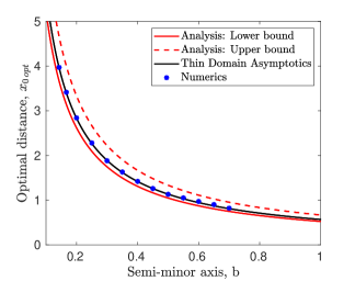
Figure 14: Three traps in an ellipse: optimal trap location (a) and optimal average MFPT (b) for a thin elliptical domain of area $\pi$ and semi-minor axis $b\ll 1$ that contains a trap centered at the origin and additional traps on either side of the origin at a distance $x_{0}$ from the center. The three traps are circular of radius $\varepsilon=0.05$. The thin domain asymptotic results in (44) (solid dark lines) are compared with full numerical results (asterisks) and the upper (red dashed lines) and lower (red solid lines) bounds based on thin-rectangle approximation.

5.3 Asymptotics of a rapidly rotating trap

In the unit disk, we analyze the two-trap problem of § 4.4 in the limit where the moving trap on the ring rotates about the center of the disk at an angular frequency $\omega\gg\mathcal{O}(\eta^{-1})$, where $\eta\ll 1$ is the radius of the moving trap. The fixed trap at the center of the disk is chosen to have a possibly different radius $\varepsilon\ll 1$. In the high frequency limit $\omega\gg 1$, the fast moving trap creates an absorbing band along its entire path as shown in Figure 15. For $\omega\gg 1$, we will calculate asymptotically the optimal radius of rotation of the moving trap in terms of $\eta$ and $\varepsilon$.

(a)    (b)

Figure 15: Optimizing the radius of rotation for a fast rotating trap in the unit disk that has a stationary trap at its center. Left: schematic plot showing the two absorbing traps in the disk. Right: MFPT for a Brownian particle with trap radii $\varepsilon=\eta=0.02$. The moving trap rotates at an angular frequency of $\omega=2000$ on a ring of radius $r=0.727$. Computed using the CPM with mesh size $\Delta x=0.005$.

We formulate the $\omega\to\infty$ limiting problem as a stationary trap problem, where the absorbing band created by the rotating trap is used to partition the unit disk into two regions, as shown in Figure 15. In the high-frequency limit $\omega\gg 1$, the limiting problem for the MFPT is to solve the multi-point BVP

(45) $$\begin{split}&u_{\rho\rho}+\rho^{-1}u_{\rho}=-{1/D}\,,\quad\mbox{in}\quad\varepsilon\leq\rho\leq r-\eta\,,\quad\mbox{and}\quad r+\eta\leq\rho<1\,,\\ &u=0\quad\mbox{on}\quad\rho=\varepsilon\,,\,\,\rho=r-\eta\,,\,\,\rho=r+\eta\,;\quad\partial_{\rho}u=0\quad\mbox{on}\quad\rho=1\,,\end{split}$$

for $u\equiv u(\rho)$. Here, we have imposed zero-Dirichlet boundary conditions on the inner and outer edges of the absorbing band created by the fast moving trap.

As detailed in § A.3 of the Supplementary Material, we first solve (45) for $u$, and then calculate the average MFPT $U(r)$ over the unit disk. This yields that

(46) $$U(r)=\frac{C}{\log\!\left(\frac{\varepsilon}{\alpha}\right)}\Big{[}\alpha^{4}-2\,\alpha^{2}\varepsilon^{2}+\varepsilon^{4}+{\left(\alpha^{4}-\beta^{4}-\varepsilon^{4}+4\,\beta^{2}-4\,\log\beta-3\right)}\log\!\left(\tfrac{\varepsilon}{\alpha}\right)\!\Big{]},$$

where $\alpha=r-\eta$, $\beta=r+\eta$, and $C$ is a constant independent of the radius of rotation $r$. To determine the optimal $r=r_{\textrm{opt}}$, we calculate numerically the root of $U^{\prime}(r_{\textrm{opt}})=0$, which is given by the zero of (A.53) in the Supplementary Material.

(a) (b)

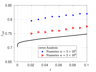
Figure 16: Optimal radius of rotation $r_{\textrm{opt}}$ for an absorbing trap of radius $\eta$ moving at constant angular frequency $\omega$ on a ring in a unit disk that contains an additional absorbing trap of radius $\varepsilon$ at the center of the disk. In (a) we fix $\eta=0.02$ and in (b) we fix $\varepsilon=0.02$. Numerical results (symbols) get closer to the asymptotic result (solid curve) for larger values of $\omega$.

In Figure 16, we show a comparison between this asymptotic result for $r_{\textrm{opt}}$ and full numerical optimization results at the two frequencies $\omega=500$ and $\omega=2000$, as obtained by using the CPM with $\Delta x=0.005$ and $\Delta r=0.001$. As expected, the asymptotic result, which is valid for $\omega\to\infty$, is seen to agree more closely with the full numerical results when $\omega=2000$ than for $\omega=500$.

In Figure 16, we show how the optimal radius of rotation of a moving trap of radius $\eta=0.02$ depends on the radius $\varepsilon$ of the stationary trap centered at the origin. We observe that the optimal rotating trap moves closer to the boundary of the unit disk as $\varepsilon$ increases. Since this increase would reduce the MFPT for particles between the two traps, the rotating trap tends to move closer to the boundary of the domain in order to reduce the MFPT for particles between the moving trap and the boundary of the unit disk. This in turn reduces the overall average MFPT. Alternatively, as the static trap radius shrinks, the optimal radius of rotation decreases and, in the limit $\varepsilon\to 0$, the optimal radius converges to $r_{\textrm{opt}}=0.7028$. Moreover, $r_{\textrm{opt}}\to{1/\sqrt{2}}\approx 0.707$ as $\eta\to 0$. This limiting radius for $\eta\to 0$ is the one that divides the unit disk into two regions of equal area, and is consistent with that given in equation (2.4) of [20].

In Figure 16, we fix the radius of the stationary trap at $\varepsilon=0.02$ and show how the optimal radius of rotation of the moving trap depends on its radius $\eta$. For this case, $r_{\textrm{opt}}$ decreases as $\eta$ increases.

6 Discussion

We have developed and implemented a Closest Point Method (CPM) to numerically compute the average MFPT for a Brownian particle in a general bounded 2-D confining domain that contains small stationary circular absorbing traps. A CPM approach was also formulated to compute the average MFPT in domain that has a mobile trap moving periodically along a concentric path within the domain. Through either a refined discrete sampling procedure or from a particle swarm optimizer routine [7], optimal trap configurations that minimize the average MFPT were identified numerically for various examples.

For the stationary trap problem with a small number of traps, some optimum trap configurations that minimize the average MFPT were computed for a class of star-shaped domains and for an elliptical domain with arbitrary aspect ratio. In particular, we have identified numerically the optimum arrangement of three traps in an ellipse of a fixed area as its boundary is deformed continuously. Under this boundary deformation we have shown that the optimal three-trap arrangement changes from a ring-pattern of traps in the unit disk to a colinear pattern of traps when the ellipse has a sufficiently large aspect ratio. Two distinct perturbation approaches were used in § 5.2 to approximate the optimal trap locations and optimal average MFPT for such a colinear trap pattern in a long, thin, ellipse.

For a class of near-disk domains with boundary $r=1+\sigma\cos(\mathcal{N}\theta)$ and $\sigma\ll 1$, we have used a perturbation approach to calculate the leading-order and ${\mathcal{O}}(\sigma)$ correction term for the average MFPT for a pattern of $m$ equally-spaced traps on a ring (i.e. ring pattern). When ${\mathcal{N}}=km$, for $k\in\mathbb{Z}^{+}$, we have shown analytically from this formula that the optimal trap locations on a ring must coincide with the maxima of the boundary deformation. Explicit results for the perturbed optimal ring radius are derived. In contrast, when ${{\mathcal{N}}/m}\notin\mathbb{Z}^{+}$, we have shown analytically that the problem of optimizing the average MFPT for a ring pattern of traps is degenerate in the sense that the ${\mathcal{O}}(\sigma)$ correction to the average MFPT vanishes for any ring radius. An open problem is to develop a hybrid asymptotic-numerical approach to identify optimal trap configurations allowing for arbitrary trap locations under an arbitrary, but small, star-shaped boundary deformation of the unit disk given by $r=1+\sigma h(\theta)$, where $\sigma\ll 1$ and $h(\theta)$ is a smooth $2\pi$ periodic function. Such a general approach could be applied to predict the initial change in the optimal locations of three traps in the ellipse as computed using the CPM in Figure 6.

An interesting mobile trap problem is path optimization: for a given domain, what is the optimal path for a trap to follow, subject to e.g., an arclength constraint? We can solve this problem numerically using the techniques developed here using constrained optimization.

Further improvements to our numerical method are possible. Our periodic moving trap problem involves relaxing over many periods; as a practical matter, we can decrease the expense by running the algorithm using an initially coarse spatial grid. After the solution has converged (in time) on the coarse grid, we can project the solution at time $t=NT$ onto a finer spatial grid and repeat.

Finally, we note the numerical algorithms described here can be applied for traps on manifolds where the Laplacian is replaced with the Laplace–Beltrami operator.

Supplementary Material: Simulation and Optimization of MFPTS. Iyaniwura, T. Wong, M. J. Ward, and C. B. Macdonald

A.1 Asymptotic analysis of the MFPT for a perturbed unit disk

We summarize the derivation of the result given in Proposition 1 of § 5.1.

We start by studying the leading-order problem (19) using the method of matched asymptotic expansions. In the inner region near each of the traps, we introduce the inner variables $\mathbf{y}=\varepsilon^{-1}(\mathbf{x}-\mathbf{x}_{j})$ and $u_{0}(\mathbf{x})=v_{j}(\varepsilon\mathbf{y}+\mathbf{x}_{j})$ with $\rho=|\mathbf{y}|$, for $j=0,\dots,m-1$. Upon writing (19) in terms of these variables, we have for $\varepsilon\to 0$ that for each $j=0,\ldots,m-1$

(A.1) $$\begin{split}\Delta_{\rho}\,v_{j}&=0\,,\quad\rho>1\,;\qquad v_{j}=0\quad\mbox{on}\quad\rho=1\,,\end{split}$$

where $\Delta_{\rho}\equiv\partial_{\rho\rho}+\rho^{-1}\partial_{\rho}$. The radially symmetric solution is $v_{j}=A_{j}\log\rho$, where $A_{j}$ for $j=0,\dots,m-1$ are constants to be determined. By matching the inner solution to the outer solution we obtain the singularity behavior of the outer solution $u_{0}$ as $\mathbf{x}\to\mathbf{x}_{j}$ for $j=0,\dots,m-1$. This leads to the following problem for $u_{0}$:

(A.2a) $$D\,\nabla^{2}u_{0}=-1\,,\quad\mathbf{x} \in\Omega\setminus\{{\mathbf{x}_{0},\ldots,\mathbf{x}_{m-1}\}}\,;\quad\partial_{r}u_{0}=0\,,\quad\mathbf{x}\in\partial\Omega\,;$$

(A.2b) $$u_{0}\sim A_{j}\log|\mathbf{x}-\mathbf{x}_{j}| +A_{j}/\nu\quad\text{as}\quad\mathbf{x}\to\mathbf{x}_{j}\qquad j=0,\dots,m-1\,.$$

Here $\nu\equiv-1/\log\varepsilon$. In terms of a Dirac forcing, this problem for $u_{0}$ is equivalent to

(A.3) $$\nabla^{2}u_{0}=-\frac{1}{D}+2\pi\sum_{j=0}^{m-1}A_{j}\delta(\mathbf{x}-\mathbf{x}_{j})\,,\qquad\partial_{r}u_{0}=0\,,\,\,\,\mathbf{x}\in\partial\Omega\,.$$

From integrating (A.3) over the unit disk, and using the divergence theorem, we get

(A.4) $$\sum_{j=0}^{m-1}A_{j}=\frac{|\Omega|}{2\pi D}\,.$$

Next, we introduce the Neumann Green’s function $G(\mathbf{x};\mathbf{x}_{j})$, which satisfies

(A.5a) $$\nabla^{2}G =\frac{1}{|\Omega|}-\delta(\mathbf{x}-\mathbf{x}_{j})\quad\mathbf{x}\in\Omega\,;\quad\partial_{n}G=0\,,\quad\mathbf{x}\in\partial\Omega\,;$$

(A.5b) $$G\sim-\frac{1}{2\pi} \log{|\mathbf{x}-\mathbf{x}_{j}|}+R_{j}+o(1)\quad\text{as}\quad\mathbf{x}\to\mathbf{x}_{j}\,;\qquad\int_{\Omega}G\,\text{d}\mathbf{x}=0\,,$$

where $R_{j}\equiv R(\mathbf{x}_{j})$ is the regular part of the Green’s function at $\mathbf{x}=\mathbf{x}_{j}$. In terms of this Green’s function, we write the solution to (A.3) as

(A.6) $$u_{0}=-2\pi\sum_{i=0}^{m-1}A_{i}G(\mathbf{x};\mathbf{x}_{i})+\overline{u}_{0}\,,$$

where $\overline{u}_{0}=(1/|\Omega|)\int_{\Omega}u_{0}\,\text{d}\mathbf{x}$ is the leading-order average MFPT. Expanding (A.6) as $\mathbf{x}\to\mathbf{x}_{j}$ for each of the traps, and using the singularity behavior of $G(\mathbf{x};\mathbf{x}_{j})$ given in (A.5b), we obtain for each $j=0,\ldots,m-1$ that

(A.7) $$u_{0}\sim A_{j}\log{|\mathbf{x}-\mathbf{x}_{j}|}-2\pi A_{j}\,R_{j}-2\pi\sum_{i\neq j}^{m-1}A_{i}\,G(\mathbf{x}_{j};\mathbf{x}_{i})+\overline{u}_{0}\,.$$

The asymptotic matching condition in this local behavior of the outer solution must agree with the behavior (A.2b) as $\mathbf{x}\to\mathbf{x}_{j}$. In this way, and recalling (A.4), we obtain an algebraic system of equations for $\overline{u}_{0},A_{0},\dots,A_{m-1}$ given in matrix form as

(A.8) $$(I+2\pi\nu\,\mathcal{G})\mathcal{A}=\nu\,\overline{u}_{0}\,\mathbf{e}\,,\qquad\mathbf{e}^{T}\mathcal{A}=\frac{|\Omega|}{2\pi D}\,.$$

Here, $\mathbf{e}\equiv(1,\dots,1)^{T}$, $\nu=-1/\log\varepsilon$, $I$ is the identity matrix, $\mathcal{A}\equiv(A_{0},\dots,A_{m-1})^{T}$, and $\mathcal{G}$ is the symmetric Green’s matrix whose entries are defined in terms of the Neumann Green’s function of (A.5) by

(A.9) $$(\mathcal{G})_{jj}=R_{j}\equiv R(\mathbf{x}_{j})\,\,\,\text{for}\,\,\,i=j\quad\text{and}\quad(\mathcal{G})_{ij}=(\mathcal{G})_{ji}=G(\mathbf{x}_{i};\mathbf{x}_{j})\,\,\,\text{for}\,\,\,i\neq j\,.$$

Since the traps are equally-spaced on the ring, the Green’s matrix $\mathcal{G}$ in (A.9) is also cyclic. Thus, from [8, Prop 4.3], $\mathbf{e}$ is an eigenvector of $\mathcal{G}$ and we have that

(A.10) $$\mathcal{G}\mathbf{e}=\kappa_{1}\mathbf{e}\,,\qquad\kappa_{1}=\frac{1}{2\pi}\left[-\log(m\,r_{c}^{m-1})-\log(1-r_{c}^{2m})+mr_{c}^{2}-\frac{3}{4}m\right]\,.$$

Then, by setting $\mathcal{A}=A_{c}\,\mathbf{e}$, for some common value $A_{c}$, in (A.8), we readily obtain

(A.11) $$A_{c}=\frac{|\Omega|}{2\pi mD}=\frac{1}{2mD},\quad\text{and}\quad\overline{u}_{0}=\frac{1}{2m\nu D}(1+2\pi\nu\kappa_{1})\,,$$

where $\kappa_{1}$ is given in (A.10). Since $\kappa_{1}\equiv\kappa_{1}(r_{c})$, any ring radius $r_{c}$ that minimizes $\kappa_{1}$ also minimizes the leading-order average MFPT $\overline{u}_{0}$. This yields the leading-order term in Proposition 1 of § 5.1.

Next, we study the $\mathcal{O}(\sigma)$ problem for $u_{1}$ given in (20). Following a similar approach used to solve the leading-order problem, we construct an inner region close to each of the traps and introduce the inner variables $\mathbf{y}=\varepsilon^{-1}(\mathbf{x}-\mathbf{x}_{j})$ and $u_{1}(\mathbf{x})=V_{j}(\varepsilon\mathbf{y}+\mathbf{x}_{j})$ with $\rho=|\mathbf{y}|$. From (20), this yields the leading-order inner problem

(A.12) $$\Delta_{\rho}\,V_{j}=0\,,\quad\rho>1\,;\qquad V_{j}=0\,,\quad\mbox{on}\,\,\,\rho=1\,,$$

where $\Delta_{\rho}\equiv\partial_{\rho\rho}+\rho^{-1}\partial_{\rho}$. The radially symmetric solution is $V_{j}=B_{j}\log\rho$, where $B_{j}$ for $j=0,\dots,m-1$ are constants to be determined. Matching this inner solution to the outer solution, we derive the singularity behavior of the outer solution $u_{1}$ as $\mathbf{x}\to\mathbf{x}_{j}$ for $j=0,\dots,m-1$. In this way, from (20), we obtain that $u_{1}$ satisfies

(A.13a) $$\nabla^{2}u_{1} =0\,,\quad\mathbf{x}\in\Omega\setminus\{\mathbf{x}_{0},\dots,\mathbf{x}_{m-1}\}\,;\quad\partial_{r}u_{1}=-hu_{0rr}+h_{\theta}u_{0\theta}\,,\quad\text{on}\quad r=1;$$

(A.13b) $$u_{1}\sim B_{j}\log{|\mathbf{x}-\mathbf{x}_{j}|}+B_{j}/\nu\quad\text{as}\quad\mathbf{x}\to\mathbf{x}_{j},\qquad j=0,\dots,m-1\,,$$

where $\nu=-1/\log\varepsilon$. To determine $u_{1}$, we need to derive its boundary condition on $r=1$ using the leading-order MFPT $u_{0}$ given in (A.6) in terms of the Neumann Green’s function $G(\mathbf{x};\mathbf{x}_{i})$. To do so, we use the Fourier series representation of the Neumann Green’s function (A.5) in the unit disk given by

(A.14) $$G(\mathbf{x};\mathbf{x}_{k})=\frac{1}{4\pi}(r^{2}+r_{c}^{2})-\frac{3}{8\pi}-\frac{1}{2\pi}\log{r_{>}}+\frac{1}{2\pi}\sum_{n=1}^{\infty}\frac{r^{n}_{<}}{n}(r_{>}^{n}+r_{>}^{-n})\cos(n(\theta-\theta_{k}))\,,$$

where $\mathbf{x}=r\,e^{i\theta}$, $\mathbf{x}_{k}=r_{c}\,e^{i(2\pi k/m+\psi)}$, $r_{>}=\max(r,r_{c})$, and $r_{<}=\min(r,r_{c})$. For any point $\mathbf{x}$ on the boundary of the unit disk, $r_{>}=r=1$, and $r_{<}=r_{c}$. Upon substituting (A.14) into (A.6), and using $A_{c}$ as given in (A.11), we conclude that

(A.15) $$u_{0}=-2\pi A_{c}\left[\frac{m}{4\pi}(1+r_{c}^{2})-\frac{3m}{8\pi}+\frac{1}{\pi}\sum_{n=1}^{\infty}\frac{r_{c}^{n}}{n}S_{n}\right]+\overline{u}_{0}\,,\quad\mbox{on}\quad r=1\,,$$

$$\text{where}\qquad S_{n}=\sum_{k=0}^{m-1} \cos(n(\theta-\theta_{k}))\,,\quad\text{with}\quad\theta_{k}=\frac{2\pi k}{m}+\psi\,.\qquad\qquad\qquad\qquad$$

To determine a Fourier series representation for $u_{0}$, we first need to sum $S_{n}$. To do so we need the following simple lemma:

Lemma .

For $d\neq 2\pi l$ for $l=0,\pm 1,\pm 2,\dots$, we have

(A.16) $$C\equiv\sum_{k=0}^{m-1}\cos(a+kd)=\frac{\sin(md/2)}{\sin(d/2)}\cos\left[a+(m-1)d/2\right]\,.$$

Proof.

We multiply both sides of (A.16) by $2\sin\left({d/2}\right)$ and use the trigonometric product-to-sum formula, $2\sin(x)\cos(y)=\sin(x+y)-\sin(x-y)$. This yields a telescoping series, which is readily summed as

$$2C\sin(d/2) =\sum_{k=0}^{m-1}2\cos(a+kd)\sin(d/2)\,,$$

$$=\sum_{k=0}^{m-1}\left(\sin\left(a+\frac{(2k+1)}{2}d\right)-\sin\left(a+\frac{(2k-1)}{2}d\right)\right)\,,$$

$$=\sin\left(a-\frac{d}{2}\right)+\sin\left(\left(a-\frac{d}{2}\right)+md\right)\,,$$

$$=2\sin\left(\frac{md}{2}\right)\cos\left[a+\frac{(m-1)d}{2}\right]\,.$$

Now, suppose that $\sin(d/2)\neq 0$, so that $d\neq 2\pi l$ for any $l=0,\pm 1,\pm 2,\dots$. Then,

$$C=\frac{\sin(md/2)}{\sin(d/2)}\cos\left[a+\frac{(m-1)d}{2}\right]\,.$$

By using Lemma A.1, we can calculate $S_{n}$, as defined in (A.15), as follows:

Lemma .

For $n\geq 1$ and $j^{\prime}=1,2,\ldots$, we have

(A.17) $$S_{n}=\begin{cases}m\cos\Big{(}j^{\prime}m(\theta-\psi)\Big{)},\quad\text{if}\quad n=j^{\prime}m\\ 0,\quad\text{if}\quad n\neq j^{\prime}m\,.\end{cases}$$

Proof.

Define $a$ and $d$ by $a=n(\theta-\psi)$ and $d=-{2\pi n/m}$. From Lemma A.1, it follows that if $d\neq 2\pi l$ for $l=0,\pm 1,\pm 2,\dots$, then $S_{n}$ satisfies

$$S_{n} =\sum_{k=0}^{m-1}\cos\Big{(}n(\theta-\psi)-\frac{2\pi nk}{m}\Big{)}=\frac{\sin(\pi n)}{\sin\left(\frac{\pi n}{m}\right)}\cos\Big{(}n(\theta-\psi)-\pi n\frac{(m-1)}{m}\Big{)}\,,$$

(A.18) $$=\frac{\sin(\pi n)}{\sin\left(\frac{\pi n}{m}\right)}\left[\cos\Big{(}n(\theta-\psi)\Big{)}\cos\Big{(}\frac{\pi n(m-1)}{m}\Big{)}+\sin\Big{(}n(\theta-\psi)\Big{)}\sin\Big{(}\frac{\pi n(m-1)}{m}\Big{)}\right]$$

This equation is valid provided that $(n/m)\neq j^{\prime}\in\{{1,2,\ldots\}}$. We observe from (A.18) that $S_{n}=0$ for $n=1,2,\dots$ with $n\neq j^{\prime}m$. Alternatively, if $n=j^{\prime}m$ for some $j^{\prime}=1,2,\ldots$, then we need to evaluate the prefactor in (A.18) using L’Hôpital’s rule. To this end, we define $g(x)\equiv\frac{\sin(\pi x)}{\sin(\pi x/m)}$, so that using L’Hôpital’s rule we get $g(x)\to{m\cos(\pi j^{\prime}m)/[\cos(\pi j^{\prime})]}$ as $x\to j^{\prime}m$. Therefore, from (A.18), we derive for $n=j^{\prime}m$ that

(A.19) $$S_{n}=\frac{m\cos(\pi j^{\prime}m)}{\cos(\pi j^{\prime})}\cos\Big{(}j^{\prime}m(\theta-\psi)\Big{)}\Big{[}\cos(\pi j^{\prime}m)\cos(\pi j^{\prime})\Big{]}=m\cos\Big{(}j^{\prime}m(\theta-\psi)\Big{)}\,.$$

Next, by substituting (A.17) for $S_{n}$, together with $A_{c}=1/(2mD)$ (see (A.11)), in (A.15), we obtain the Fourier series representation for $u_{0}$ on $r=1$ given by

(A.20) $$\begin{split}\qquad u_{0}&=c_{0}+\sum_{j^{\prime}=1}^{\infty}c_{j^{\prime}}\cos\big{(}j^{\prime}m(\theta-\psi)\big{)}\,,\quad\mbox{on}\,\,\,r=1\,,\\ \text{where}\quad c_{0}&=-\frac{1}{8D}\Big{(}2(1+r_{c}^{2})-3\Big{)}+\overline{u}_{0}\,;\qquad c_{j^{\prime}}=-\frac{r_{c}^{j^{\prime}m}}{j^{\prime}mD}\,,\quad j^{\prime}=1,2,\ldots\,.\end{split}$$

We return to the $\mathcal{O}(\sigma)$ outer problem (A.13) for $u_{1}$ and simplify the boundary condition on $r=1$ given in (A.13a) as $u_{1r}=F(\theta)\equiv-hu_{0rr}+h_{\theta}u_{0\theta}$ on $r=1$. Since $u_{0}$ satisfies the MFPT PDE, in polar coordinates we have that $u_{0rr}+r^{-1}u_{0r}+r^{-2}u_{0\theta\theta}=-1/D$. Evaluating this on $r=1$ where $u_{0r}=0$, we get that $u_{0rr}=-u_{0\theta\theta}-1/D$ on $r=1$. Upon substituting this expression for $u_{0rr}$ into $F(\theta)$, we derive

(A.21) $$u_{1r}=F(\theta)=(hu_{0\theta})_{\theta}+\frac{h}{D}\,,\quad\text{on}\quad r=1\,,$$

where $u_{0}$ on $r=1$ is given in (A.20) and $h(\theta)=\cos(\mathcal{N}\theta)$.

Next, we write the problem (A.13) for $u_{1}$ as

(A.22) $$\nabla^{2}u_{1}=2\pi\sum_{i=0}^{m-1}B_{i}\,\,\delta(\mathbf{x}-\mathbf{x}_{i})\,,\quad\mathbf{x}\in\Omega\,;\qquad u_{1r}=F(\theta)\,,\quad\text{on}\quad r=1\,.$$

Integrating (A.22) over the unit disk, and using the divergence theorem and the fact that $\int_{0}^{2\pi}F(\theta)\,\text{d}\theta=0$, we conclude that $\sum_{j=0}^{m-1}B_{j}=0$. It is then convenient to decompose $u_{1}$ as

(A.23) $$u_{1}=u_{1H}+u_{1p}+\overline{u}_{1}\,,$$

where the unknown constant $\overline{u}_{1}$ is the average of $u_{1}$ over the unit disk. Here, $u_{1H}$ is taken to be the unique solution to

(A.24) $$\nabla^{2}u_{1H}=2\pi\sum_{i=0}^{m-1}B_{i}\,\delta(\mathbf{x}-\mathbf{x}_{i})\,,\quad\mathbf{x}\in\Omega\,;\quad\partial_{r}u_{1H}=0\,,\quad\text{on}\quad r=1\,;\quad\int_{\Omega}u_{1H}\,\text{d}\mathbf{x}=0\,.$$

In addition, $u_{1p}$ is defined to be the unique solution to

(A.25) $$\nabla^{2}u_{1p} =0,\quad\mathbf{x}\in\Omega;\quad\partial_{r}u_{1p}=F(\theta)\,\quad\text{on}\quad r=1;\quad\int_{\Omega}u_{1p}\,\text{d}\mathbf{x}=0\,,$$

which is readily solved using separation of variables once $F(\theta)$ is represented as a Fourier series.

The solution to (A.24) is represented in terms of the Neumann Green’s function $G(\mathbf{x};\mathbf{x}_{i})$ of (A.5), so that

(A.26) $$u_{1}=-2\pi\sum_{i=0}^{m-1}B_{i}G(\mathbf{x};\mathbf{x}_{i})+u_{1p}+\overline{u}_{1}.$$

Expanding (A.26) as $\mathbf{x}\to\mathbf{x}_{j}$, and using the singularity behavior of $G(\mathbf{x};\mathbf{x}_{j})$ as given in (A.5b), we derive the local behavior of $u_{1}$ as $\mathbf{x}\to\mathbf{x}_{j}$, for each $j=0,\ldots,m-1$, which must agree with that given in (A.13b). This yields an $(m+1)$ dimensional algebraic system of equations for the constants $B_{0},\dots,B_{m-1}$ and $\overline{u}_{1}$ given in matrix form by

(A.27) $$(I+2\pi\nu\mathcal{G})\mathbf{B}=\nu\overline{u}_{1}\mathbf{e}+\nu\mathbf{u}_{1p}\,,\qquad\mathbf{e}^{T}\mathbf{B}=0\,.$$

Here, $I$ is the $m\times m$ identity matrix, $\mathbf{B}=(B_{0},\dots,B_{m-1})^{T}$, $\mathbf{e}=(1,\dots,1)^{T}$, and $\mathbf{u}_{1p}=(u_{1p}(\mathbf{x}_{0}),\dots,u_{1p}(\mathbf{x}_{m-1}))^{T}$. Upon multiplying this equation for $\mathbf{B}$ on the left by $\mathbf{e}^{T}$, we can isolate $\overline{u}_{1}$ as

$$\nu\,\overline{u}_{1}=\frac{1}{m}\Big{(}2\pi\nu\mathbf{e}^{T}\mathcal{G}\mathbf{B}-\nu\mathbf{e}^{T}\mathbf{u}_{1p}\Big{)}\,.$$

Upon re-substituting this expression into (A.27), we conclude that $\mathbf{e}^{T}\mathbf{B}=0$ and that

(A.28) $$\Big{[}I+2\pi\nu(I-E)\mathcal{G}\Big{]}\mathbf{B}=\nu(I-E)\mathbf{u}_{1p}\,,\quad\text{and}\quad\overline{u}_{1}=-\frac{1}{m}\Big{(}\mathbf{e}^{T}\mathbf{u}_{1p}-2\pi\mathbf{e}^{T}\mathcal{G}\mathbf{B}\Big{)}\,,$$

where we have defined $E={\mathbf{e}\mathbf{e}^{T}/m}$. This gives an equation for the $\mathcal{O}(\sigma)$ average MFPT $\overline{u}_{1}$ in terms of the Neumann Green’s matrix $\mathcal{G}$, and the vectors $\mathbf{B}$ and $\mathbf{u}_{1p}$.

The next step in this calculation is to solve (A.25) so as to calculate $u_{1p}(\mathbf{x}_{j})$ for $j=0,\ldots,m-1$. To do so, we first need to find an explicit Fourier series representation for $F(\theta)$, as defined in (A.21) in terms of $u_{0}$ on $r=1$.

By using (A.20) for $u_{0}$ on $r=1$, together with $h=\cos(\mathcal{N}\theta)$, we calculate that

$$\begin{split}hu_{0\theta}&=-\frac{\cos(\mathcal{N}\psi)}{2}\sum_{j^{\prime}=1}^{\infty}c_{j^{\prime}}j^{\prime}m\Big{[}\sin\Big{(}(j^{\prime}m+\mathcal{N})(\theta-\psi)\Big{)}+\sin\Big{(}(j^{\prime}m-\mathcal{N})(\theta-\psi)\Big{)}\Big{]}\\ &+\frac{\sin(\mathcal{N}\psi)}{2}\sum_{j^{\prime}=1}^{\infty}c_{j^{\prime}}j^{\prime}m\Big{[}\cos\Big{(}(j^{\prime}m-\mathcal{N})(\theta-\psi)\Big{)}-\cos\Big{(}(j^{\prime}m+\mathcal{N})(\theta-\psi)\Big{)}\Big{]}\,.\end{split}$$

Upon differentiating this expression with respect to $\theta$, we obtain after some algebra that

(A.29) $$\Big{(}h(\theta)u_{0\theta}\Big{)}_{\theta}=-\sum_{j^{\prime}=1}^{\infty}\frac{c_{j^{\prime}}j^{\prime}m}{2}\Big{[}j^{\prime}_{+}\cos\Big{(}j^{\prime}_{+}(\theta-\psi)+\mathcal{N}\psi\Big{)}+j^{\prime}_{-}\cos\Big{(}j^{\prime}_{-}(\theta-\psi)-\mathcal{N}\psi\Big{)}\Big{]}\,,$$

where we have defined $j^{\prime}_{\pm}$ by $j^{\prime}_{\pm}=j^{\prime}m\pm\mathcal{N}$. Upon substituting (A.29) into (A.21), and recalling that $c_{j^{\prime}}=-(r_{c}^{j^{\prime}m})/(j^{\prime}mD)$, we conclude that

(A.30) $$F(\theta)=\frac{1}{D}\cos(\mathcal{N}\theta)+\frac{1}{2D}\sum_{j^{\prime}=1}^{\infty}r_{c}^{j^{\prime}m}\Big{[}j^{\prime}_{+}\cos\Big{(}j^{\prime}_{+}(\theta-\psi)+\mathcal{N}\psi\Big{)}+j^{\prime}_{-}\cos\Big{(}j^{\prime}_{-}(\theta-\psi)-\mathcal{N}\psi\Big{)}\Big{]}\,.$$

With $F(\theta)$ as given in (A.30), by separation of variables the solution $u_{1}$ to (A.25) that is bounded as $r\to 0$ is

(A.31) $$\begin{split}u_{1p}&=\sum_{\begin{subarray}{c}j^{\prime}=1\\ j^{\prime}_{-}\neq\,0\end{subarray}}^{\infty}\frac{r_{c}^{j^{\prime}m}}{2D}\Big{[}r^{j^{\prime}_{+}}\cos\Big{(}j^{\prime}_{+}(\theta-\psi)+\mathcal{N}\psi\Big{)}+\gamma\,r^{|j^{\prime}_{-}|}\cos\Big{(}j^{\prime}_{-}(\theta-\psi)-\mathcal{N}\psi\Big{)}\Big{]}\\ &\qquad+\frac{r^{\mathcal{N}}\cos(\mathcal{N}\theta)}{\mathcal{N}D}\,,\end{split}$$

where $\gamma=\text{sign}(j^{\prime}_{-})$, $m$ is the number of traps on the ring of radius $r_{c}$, and $\mathcal{N}$ is the number of folds on the star-shaped domain. If $\mathcal{N}>m$, then $j^{\prime}_{-}<0$ at least for $j^{\prime}=1$, while when $\mathcal{N}=m$ then $j^{\prime}_{-}=0$ when $j^{\prime}=1$.

Next, using the explicit solution (A.31), we calculate $u_{1p}$ at the centers of the traps given by $\mathbf{x}_{j}=r_{c}\,\exp{\Big{(}(2\pi j/m+\psi)i\Big{)}}$ for $j=0,\ldots,m-1$. At $\mathbf{x}=\mathbf{x}_{j}$, we have $\theta=2\pi{j/m}+\psi$, so that $\cos(\mathcal{N}\theta)=\cos\Big{(}\mathcal{N}\psi+2\pi j\mathcal{N}/m\Big{)}$. Similarly, we obtain

(A.32) $$\cos\Big{(}j^{\prime}_{+}(\theta-\psi)+\mathcal{N}\psi\Big{)}=\cos\Big{(}j^{\prime}_{-}(\theta-\psi)-\mathcal{N}\psi\Big{)}=\cos\Big{(}\mathcal{N}\psi+2\pi j\mathcal{N}/m\Big{)}\,.$$

Upon evaluating (A.31) at $\mathbf{x}=\mathbf{x}_{j}$ and using (A.32), we obtain that

(A.33) $$u_{1p}(\mathbf{x}_{j})=\frac{r_{c}^{\mathcal{N}}}{2D}\cos\left(\mathcal{N}\Big{(}\psi+\frac{2\pi j}{m}\Big{)}\right)\left[\frac{2}{\mathcal{N}}+\sum_{j^{\prime}=1}^{\infty}r_{c}^{2mj^{\prime}}+\sum_{\begin{subarray}{c}j^{\prime}=1\\ j^{\prime}_{-}\neq\,0\end{subarray}}^{\infty}\text{sign}(j^{\prime}_{-})r_{c}^{(j^{\prime}m+|j^{\prime}_{-}|-\mathcal{N})}\right]$$

for $j=0,\ldots,m-1$. This expression is used to determine the vector $\mathbf{u}_{1p}$ in (A.28). Observe from (A.33) that $u_{1p}(\mathbf{x}_{j})$ is independent of $j$ when $\mathcal{N}/m$ is a positive integer. In other words, $u_{1p}$ is independent of the location of the traps when the number of folds $\mathcal{N}$ of the perturbation of the boundary is an integer multiple of the number of traps $m$ contained in the domain.

Finally, upon substituting $h(\theta)=\cos(\mathcal{N}\theta)$ and $u_{0}$, as given in (A.20), into (21), we can evaluate the third integral in (21). In this way, we conclude that a two-term expansion in $\sigma$ for the average MFPT $\overline{u}$ is

(A.34) $$\begin{split}\overline{u}\sim\overline{u}_{0}+\sigma\overline{u}_{1}+\begin{cases}0,\quad&\text{if}\quad(\mathcal{N}/m)\notin\mathbb{Z}^{+}\\ -\sigma\Big{(}r_{c}^{\mathcal{N}}\cos(\mathcal{N}\psi)\Big{)}/(\mathcal{N}D),\quad&\text{if}\quad(\mathcal{N}/m)\in\mathbb{Z}^{+}\end{cases}\,,\end{split}$$

where $\mathbb{Z}^{+}$ is the set of positive integers. Here $\overline{u}_{0}$ and $\overline{u}_{1}$ are the leading-order and $\mathcal{O}(\sigma)$ average MFPT given by (A.11) and the solution to (A.28), respectively.

The remainder of the calculation depends on whether ${\mathcal{N}/m}\in\mathbb{Z}^{+}$ or ${\mathcal{N}/m}\notin\mathbb{Z}^{+}$. We will consider both cases separately.

A.1.1 Number of folds is an integer multiple of the number of traps: $(\mathcal{N}=km)$

When the number of folds on the star-shaped domain is an integer multiple of the number of traps contained in the domain, then, from (A.33), we conclude that $u_{1p}(\mathbf{x}_{j})$ is independent of $j$. Therefore, using (A.33) and noting that $j_{-}=(j^{\prime}-k)m$ and $\text{sign}(j_{-})=\text{sign}(j^{\prime}-k)$, we calculate $\mathbf{u}_{1p}=(u_{1p}(\mathbf{x}_{0}),\dots,u_{1p}(\mathbf{x}_{m-1}))^{T}$ as

(A.35) $$\begin{split}\mathbf{u}_{1p}&\equiv u_{1pc}\,\mathbf{e}\,,\quad\text{with}\quad u_{1pc}=\frac{1}{D}\cos(m\psi)\,\chi\,,\\ \text{where}\quad\chi&\equiv\frac{r_{c}^{\mathcal{N}}}{\mathcal{N}}+\frac{1}{2}r_{c}^{\mathcal{N}}\sum_{j^{\prime}=1}^{\infty}r_{c}^{2mj^{\prime}}-\frac{1}{2}\sum_{j^{\prime}=1}^{k-1}r_{c}^{j^{\prime}m+m(k-j^{\prime})}+\frac{1}{2}\sum_{j^{\prime}=k+1}^{\infty}r_{c}^{j^{\prime}m+m(j^{\prime}-k)}\,.\end{split}$$

We observe that the third term in $\chi$ is proportional to $(k-1)$, and that we can combine the second and fourth terms into a single geometric series by shifting indices. In this way, and by using $mk=\mathcal{N}$, we can calculate $\chi$ explicitly as

(A.36) $$\chi=r_{c}^{\mathcal{N}}\left(\frac{1}{\mathcal{N}}-\frac{1}{2}(k-1)\right)+r_{c}^{\mathcal{N}}\sum_{j^{\prime}=1}^{\infty}r_{c}^{2j^{\prime}m}=r_{c}^{\mathcal{N}}\left(\frac{1}{\mathcal{N}}-\frac{1}{2}(k-1)\right)+\frac{r_{c}^{\mathcal{N}+2m}}{1-r_{c}^{2m}}\,.$$

Substituting (A.35) into (A.28), and noting that $(I-E)\mathbf{u}_{1p}=0$ and that the matrix $(I+2\pi\nu(I-E)\mathcal{G})$ is invertible, we conclude that $\mathbf{B}=\mathbf{0}$. Therefore, from (A.28) we get that $\overline{u}_{1}=-u_{1pc}$. In this way, by using (A.35), (A.36), and (A.34) we obtain that the ${\mathcal{O}}(\sigma)$ correction, denoted by $\overline{U}_{1}$, to the average MFPT is

(A.37) $$\overline{U}_{1}\equiv-u_{1pc}-\frac{\Big{(}r_{c}^{\mathcal{N}}\cos(\mathcal{N}\psi)\Big{)}}{\mathcal{N}D}=-\frac{\cos(\mathcal{N}\psi)}{D}\left(\frac{2r_{c}^{\mathcal{N}}}{\mathcal{N}}-\frac{r_{c}^{\mathcal{N}}}{2}(k-1)+\frac{r_{c}^{\mathcal{N}+2m}}{1-r_{c}^{2m}}\right)\,.$$

Finally, by combining the terms in (A.37) we obtain the main result given in Proposition 1 of § 5.1.

A.1.2 Number of folds is not an integer multiple of the number of traps: $(\mathcal{N}\neq km)$

When ${\mathcal{N}/m}\notin\mathbb{Z}^{+}$, we will first establish that $\mathbf{e}^{T}\mathbf{u}_{1p}=0$. To show this, we define $z\equiv e^{2\pi i\mathcal{N}/m}$, where $i=\sqrt{-1}$, and calculate that

$$\sum_{j=0}^{m-1}\cos\left(\mathcal{N}\psi+\frac{2\pi j\mathcal{N}}{m}\right)=\mbox{Re}\left(e^{i\mathcal{N}\psi}\sum_{j=0}^{m-1}z^{j}\right)=\mbox{Re}\left(e^{i\mathcal{N}\psi}\frac{(1-z^{m})}{1-z}\right)=0\,,$$

since $z^{m}=1$ but $z\neq 1$, owing to the fact that ${\mathcal{N}/m}\neq\mathbb{Z}^{+}$. As a result, by summing the terms in (A.33) over $j$, we obtain that $\mathbf{e}^{T}\mathbf{u}_{1p}=0$. We conclude that $\mathbf{u}_{1p}\in{\mathcal{Q}}$, where ${\mathcal{Q}}\equiv\{{\mathbf{q}\in\mathbb{R}^{m-1}\,\,|\,\,\mathbf{q}^{T}\mathbf{e}=0\}}$. Consequently, from (A.28), the problem for $\mathbf{B}$ and $\overline{u}_{1}$ reduces to

(A.38) $$\Big{[}I+2\pi\nu(I-E)\mathcal{G}\Big{]}\mathbf{B}=\nu\mathbf{u}_{1p}\,,\quad\text{and}\quad\overline{u}_{1}=\frac{2\pi}{m}\mathbf{e}^{T}\mathcal{G}\mathbf{B}\,.$$

Next, since the Neumann Green’s matrix $\mathcal{G}$ is cyclic and symmetric, its matrix spectrum is given by

(A.39) $$\mathcal{G}\mathbf{e}=\kappa_{1}\mathbf{e}\,;\qquad\mathcal{G}\mathbf{q}_{j}=\kappa_{j}\mathbf{q}_{j}\,,\quad j=2,\ldots,m\,,$$

where $\mathbf{q}_{j}^{T}\mathbf{q}_{i}=0$ for $i\neq j$ and $\mathbf{e}^{T}\mathbf{q}_{j}=0$ for $j=2,\ldots,m$. Therefore, the set $\{{\mathbf{q}_{2},\ldots,\mathbf{q}_{m}\}}$ forms an orthogonal basis for the subspace ${\mathcal{Q}}$. As such, since $\mathbf{u}_{1p}\in{\mathcal{Q}}$, we have $\mathbf{u}_{1p}=\sum_{j=2}^{m}d_{j}\mathbf{q}_{j}$, for some coefficients $d_{j}$, for $j=2,\ldots,m$, and we can seek a solution for $\mathbf{B}$ in (A.38) in the form $\mathbf{B}=\sum_{j=2}^{m}b_{j}\mathbf{q}_{j}$ for some $b_{j}$, $j=2,\ldots,m$. Since $E\mathbf{q}_{j}=0$, we readily calculate that

(A.40) $$\mathbf{B}=\nu\sum_{j=2}^{m}\frac{d_{j}}{1+2\pi\nu\kappa_{j}}\mathbf{q}_{j}\,,\qquad\mbox{where}\qquad d_{j}=\frac{\mathbf{q_{j}}^{T}\mathbf{u}_{1p}}{\mathbf{q_{j}}^{T}\mathbf{q}_{j}}\,.$$

Then, since $\mathcal{G}\mathbf{B}\in{\mathcal{Q}}$ and $\mathbf{e}^{T}\mathbf{q}=0$ for $\mathbf{q}\in{\mathcal{Q}}$, it follows that $\mathbf{e}^{T}\mathcal{G}\mathbf{B}=0$ so that $\overline{u}_{1}=0$ in (A.38). Finally, in view of (A.34), we conclude that the correction of order ${\mathcal{O}}(\sigma)$ in the average MFPT vanishes. This establishes the result given in Proposition 1 of § 5.1 when ${\mathcal{N}/m}\notin\mathbb{Z}^{+}$.

A.2 Approximations for optimal trap configurations in a thin ellipse

We provide some details for the two different approximation schemes outlined in § 5.2 for estimating the optimal average MFPT for an elliptical domain of high-eccentricity that contains three traps centered along the semi-major axis.

A.2.1 Equivalent thin rectangular domains: Three traps

We extend the calculation of § 5.2.1 to the case of three circular absorbing traps of a common radius $\varepsilon$, where one of the traps is located at the center of the ellipse, while the other two traps are centered on the major axis symmetric about the origin.

We follow a similar approach as for the two traps case in § 5.2.1, where we replace the ellipse with a thin rectangular region, chosen so that the area of the region and that of the traps is preserved. The corresponding MFPT problem on the rectangle is to solve (32) with the additional requirement that $u=0$ for $x=\pm\varepsilon_{0}$ on $|y|\leq b$. Upon calculating the 1-D solution $u(x)$ to this MFPT problem, we then integrate it over the rectangle to determine the average MFPT $\overline{u}$ as

(A.41) $$\overline{u}=C\left(-\frac{1}{4}\,x_{0}^{3}+\frac{1}{2}\,{\left(2\,a_{0}-3\,\varepsilon_{0}\right)}x_{0}^{2}-{\left(a_{0}^{2}-2\,a_{0}\varepsilon_{0}\right)}x_{0}+\frac{1}{3}\,a_{0}^{3}-a_{0}^{2}\varepsilon_{0}+a_{0}\varepsilon_{0}^{2}-\varepsilon_{0}^{3}\right)\,,$$

where $C={4\,b_{0}/\left[\pi\,D\,(1-3\varepsilon^{2})\right]}$ and $x_{0}$ is the $x$-coordinate of the right-most trap.

To determine the optimal average MFPT as $x_{0}$ is varied, we set ${d\overline{u}/dx_{0}}=0$ in (A.41). The critical point that minimizes the average MFPT is

(A.42) $$x_{0\,{\textrm{opt}}}=\frac{2a_{0}}{3}=\frac{\pi}{6\,b_{0}}\,,$$

where we used $a_{0}={\pi/(4b_{0})}$ from (33). This gives the optimal trap locations as $(\pm 2a_{0}/3,0)$. As compared to the result in § 5.2.1 for two traps, the optimal traps have moved closer to the reflecting boundaries at $x=\pm a_{0}$. Upon substituting (A.42) into (A.41), and writing $a_{0}$ and $\varepsilon_{0}$ in terms of the width of the rectangular region $b_{0}$ using the equal area condition (33), we obtain that the optimal average MFPT for the rectangle is

(A.43) $$\overline{u}_{\textrm{opt}}=\frac{\pi^{2}}{432\,D\,b_{0}^{2}}\Big{(}1-6\,\varepsilon^{2}+\mathcal{O}(\varepsilon^{4})\Big{)}.$$

This shows that $\overline{u}_{\textrm{opt}}=\mathcal{O}(b_{0}^{-2})$, and as expected, the optimal average MFPT is smaller than that in (35) of § 5.2.1 for the case of two traps.

To relate the optimal MFPT in the thin rectangular domain to that in the thin elliptical domain, we proceed as in § 5.2.1 for the two-trap case. We first set $a=a_{0}$, so that the length of the rectangular domain and the ellipse along the major axis are the same. From (33), we obtain $b_{0}=(\pi b)/4$, where $b$ is the semi-minor axis of the ellipse, and so (A.42) and (A.43) become

(A.44) $$x_{0\,{\textrm{opt}}}=\frac{2}{3b}\quad\mbox{and}\quad\overline{u}_{\textrm{opt}}\approx\frac{1}{27\,D\,b^{2}}\Big{(}1-6\,\varepsilon^{2}+\mathcal{O}(\varepsilon^{4})\Big{)}\,;\qquad\mbox{Case I:}\,\,\,(a=a_{0})\,.$$

The second possibility is to choose $b=b_{0}$, so that the width of the thin rectangle and ellipse are the same. From (A.42) and (A.43), we get

(A.45) $$x_{0\,{\textrm{opt}}}=\frac{\pi}{6b}\quad\mbox{and}\quad\overline{u}_{\textrm{opt}}\approx\frac{\pi^{2}}{432\,D\,b^{2}}\Big{(}1-6\,\varepsilon^{2}+\mathcal{O}(\varepsilon^{4})\Big{)}\,;\qquad\mbox{Case II:}\,\,\,(b=b_{0})\,.$$

Similarly to the two-trap case, the results in (A.44) and (A.45) provide upper and lower bounds, respectively, for the optimal locations of the trap and the optimal average MFPT in the thin elliptical region.

A.2.2 A perturbation approach for long thin domains

In the asymptotic limit of a long thin domain, we use a perturbation approach on the MFPT PDE (39) in § 5.2.2 for $u(x,y)$ in order to derive the limiting problem (40).

We first introduce the stretched variables $x$ and $y$ by $X=\delta x,Y={y/\delta}$ and $d={x_{0}/\delta}$, and we label $U(X,Y)=u({X/\delta},Y\delta)$. Then the PDE in (39) becomes

(A.46) $$\delta^{4}\partial_{XX}U+\partial_{YY}U=-\frac{\delta^{2}}{D}\,.$$

For $\delta\ll 1$, this suggests an expansion of $u$ given by

(A.47) $$U=\delta^{-2}U_{0}+U_{1}+\delta^{2}U_{2}+\ldots\,.$$

Upon substituting (A.47) into (A.46), and equating powers of $\delta$, we obtain

(A.48) $${\mathcal{O}}(\delta^{-2})\,: \quad\partial_{YY}U_{0}=0\,,$$

$${\mathcal{O}}(1)\,: \quad\partial_{YY}U_{1}=0\,,$$

$${\mathcal{O}}(\delta^{2})\,: \quad\partial_{YY}U_{2}=-\frac{1}{D}-\partial_{XX}U_{0}\,.$$

On the boundary $y=\pm\delta F(\delta x)$, or equivalently $Y=\pm F(X)$, the unit outward normal is $\hat{\mathbf{n}}={\mathbf{n}/|\mathbf{n}|}$, where $\mathbf{n}\equiv(-\delta^{2}F^{\prime}(X),\pm 1)$. The condition for the vanishing of the outward normal derivative in (39) becomes

$$\partial_{n}u=\hat{\mathbf{n}}\cdot(\partial_{x}u,\partial_{y}u)=\frac{1}{|\mathbf{n}|}(-\delta^{2}F^{\prime},\pm 1)\cdot(\delta\partial_{X}U,\delta^{-1}\partial_{Y}U)=0\,,\,\,\,\mbox{on}\,\,\,Y=\pm F(X)\,.$$

This is equivalent to the condition that

(A.49) $$\partial_{Y}U=\pm\delta^{4}F^{\prime}(X)\partial_{X}U\quad\mbox{on}\quad Y=\pm F(X)\,.$$

Upon substituting (A.47) into (A.49) and equating powers of $\delta$ we obtain on $Y=\pm F(X)$ that

(A.50) $${\mathcal{O}}(\delta^{-2})\,: \quad\partial_{Y}U_{0}=0\,,$$

$${\mathcal{O}}(1)\,; \quad\partial_{Y}U_{1}=0\,,$$

$${\mathcal{O}}(\delta^{2})\,; \quad\partial_{Y}U_{2}=\pm F^{\prime}(X)\partial_{X}U_{0}\,.$$

From (A.48) and (A.50) we conclude that $U_{0}=U_{0}(X)$ and $U_{1}=U_{1}(X)$. Assuming that the trap radius $\varepsilon$ is comparable to the domain width $\delta$ we will approximate the zero Dirichlet boundary condition on the three traps as zero point constraints for $U_{0}$ at $X=0,\pm d$.

A multi-point BVP for $U_{0}(X)$ is derived by imposing a solvability condition on the ${\mathcal{O}}(\delta^{2})$ problem for $U_{2}$ given by

(A.51) $$\partial_{YY}U_{2}=-\frac{1}{D}-U_{0}^{\prime\prime}\,,\,\,\,\mbox{in}\,\,\,\Omega\setminus\Omega_{a}\,;\quad\partial_{Y}U_{2}=\pm F^{\prime}(X)U_{0}^{\prime}\,,\,\,\,\mbox{on}\,\,\,Y=\pm F(X)\,,\,\,|X|<1\,.$$

To derive this solvability condition for (A.51), we multiply the problem for $U_{2}$ by $U_{0}$ and integrate in $Y$ over $-F(X)<Y<F(X)$. Upon using Lagrange’s identity and the boundary conditions in (A.51) we get

(A.52) $$\int_{-F(X)}^{F(X)}\left(U_{0}\partial_{YY}U_{2}-U_{2}\partial_{YY}U_{0}\right)\,\text{d}Y =\left[U_{0}\partial_{Y}U_{2}-U_{2}\partial_{Y}U_{0}\right]\Big{|}_{-F(X)}^{F(X)}\,,$$

$$\int_{-F(X)}^{F(X)}U_{0}\left(-\frac{1}{D}-U_{0}^{\prime\prime}\right)\,\text{d}Y =2U_{0}F^{\prime}(X)U_{0}^{\prime}\,,$$

$$2F(X)U_{0}\left(-\frac{1}{D}-U_{0}^{\prime\prime}\right) =2U_{0}F^{\prime}(X)U_{0}^{\prime}\,.$$

Thus, $U_{0}(X)$ satisfies the ODE $\left[F(X)U_{0}^{\prime}\right]^{\prime}=-{F(X)/D}$ as given in (40) of § 5.2.2.

A.3 Asymptotic analysis of a fast rotating trap

We summarize the derivation of the result given in § 5.3 for the optimal radius of rotation of the rotating trap problem of § 4.4 in the limit of fast rotation $\omega\gg 1$. In this limit, the asymptotic MFPT $u(\rho)$ satisfies the multi-point BVP (45), which has the solution

$$u =\frac{1}{4}\Big{(}(r-\eta)^{2}-\rho^{2}\Big{)}+\frac{1}{4\log\left(\frac{\varepsilon}{r-\eta}\right)}\left[(\varepsilon^{2}-(r-\eta)^{2})\log\left(\frac{\rho}{r-\eta}\right)\right]\,,\,\,\,\varepsilon\leq\rho\leq r-\eta\,,$$

$$u =\frac{1}{4}((r+\eta)^{2}-\rho^{2})+\frac{1}{2}\log\left(\frac{\rho}{r+\eta}\right)\,,\,\,\,r+\eta\leq\rho\leq 1\,.$$

To compute the average MFPT, denoted by $U(r)$, over the unit disk, we need to calculate $I=\int_{0}^{r-\eta}u\rho\,\text{d}\rho+\int_{r+\eta}^{1}u\rho\,\text{d}\rho$. By doing so, we obtain that $U(r)$ is given in (46). To optimize the average MFPT with respect to the radius of rotation of the fast moving trap, we simply set $U^{\prime}(r)=0$. This leads to the following transcendental equation for $r$ in terms of the radii $\eta$ and $\varepsilon$ of the two traps:

(A.53) $$\mathcal{A}(r)+4\mathcal{B}(r)\log\left(\frac{\varepsilon}{r-\eta}\right)^{2}-4\log\left(\frac{\varepsilon}{r-\eta}\right)\mathcal{C}(r)=0\,.$$

Here $\mathcal{A}(r)$, $\mathcal{B}(r)$, and $\mathcal{C}(r)$ are defined by

$$\mathcal{A}(r) =\varepsilon^{4}\eta-2\,\varepsilon^{2}\eta^{3}+\eta^{5}-3\,\eta r^{4}+r^{5}-2\,\left(\varepsilon^{2}-\eta^{2}\right)r^{3}+2\,\left(\varepsilon^{2}\eta+\eta^{3}\right)r^{2}$$

$$\qquad+\left(\varepsilon^{4}+2\,\varepsilon^{2}\eta^{2}-3\,\eta^{4}\right)r\,,$$

$$\mathcal{B}(r) =2\,\eta^{5}-6\,\eta r^{4}-2\,\eta^{3}+2\,\left(2\,\eta^{3}+\eta\right)r^{2}+2\,r^{3}-\left(2\,\eta^{2}+1\right)r+\eta\,,$$

$$\mathcal{C}(r) =\varepsilon^{2}\eta^{3}-\eta^{5}+3\,\eta r^{4}-r^{5}+\left(\varepsilon^{2}-2\,\eta^{2}\right)r^{3}-\left(\varepsilon^{2}\eta+2\,\eta^{3}\right)r^{2}-\left(\varepsilon^{2}\eta^{2}-3\,\eta^{4}\right)r\,.$$

To determine the optimal $r$ we need to numerically compute the root of (A.53). The results were shown in Figure 16.

References

• [1] Y. Chen and C. B Macdonald. The closest point method and multigrid solvers for elliptic equations on surfaces. SIAM J. Sci. Comput., 37(1):A134–A155, 2015.
• [2] A. F Cheviakov, M. J Ward, and R. Straube. An asymptotic analysis of the mean first passage time for narrow escape problems: Part ii: The sphere. SIAM J. Multiscale Model. Simul., 8(3), 2010.
• [3] D. Coombs, R. Straube, and M. Ward. Diffusion on a sphere with localized traps: Mean first passage time, eigenvalue asymptotics, and fekete points. SIAM J. Appl. Math., 70(1), 2009.
• [4] Björn Engquist, Anna-Karin Tornberg, and Richard Tsai. Discretization of dirac delta functions in level set methods. Journal of Computational Physics, 207(1):28–51, 2005.
• [5] I. V Grigoriev, Y. A Makhnovskii, A. M Berezhkovskii, and V. Yu Zitserman. Kinetics of escape through a small hole. The Journal of chemical physics, 116(22):9574–9577, 2002.
• [6] D. Holcman and Z. Schuss. Escape through a small opening: receptor trafficking in a synaptic membrane. Journal of Statistical Physics, 117(5-6):975–1014, 2004.
• [7] James Kennedy. Particle swarm optimization. Encyclopedia of machine learning, pages 760–766, 2010.
• [8] T. Kolokolnikov, M. S Titcombe, and M. J Ward. Optimizing the fundamental Neumann eigenvalue for the Laplacian in a domain with small traps. European Journal of Applied Mathematics, 16(2):161–200, 2005.
• [9] V. Kurella, J. C Tzou, D. Coombs, and M. J Ward. Asymptotic analysis of first passage time problems inspired by ecology. Bulletin of Mathematical Biology, 77(1), 2015.
• [10] A. E Lindsay, J. C Tzou, and T. Kolokolnikov. Optimization of first passage times by multiple cooperating mobile traps. SIAM J. Multiscale Model. Simul., 15(2), 2017.
• [11] C. B Macdonald, J. Brandman, and S. J Ruuth. Solving eigenvalue problems on curved surfaces using the closest point method. J. Comput. Phys., 230(22), 2011.
• [12] C. B. Macdonald, B. Merriman, and S. J. Ruuth. Simple computation of reaction-diffusion processes on point clouds. Proc. Natl. Acad. Sci., 110(23), 2013.
• [13] C. B Macdonald and S. J Ruuth. The implicit closest point method for the numerical solution of partial differential equations on surfaces. SIAM J. Sci. Comput., 31(6), 2009.
• [14] L. Mirny, M. Slutsky, Z. Wunderlich, A. Tafvizi, J. Leith, and A. Kosmrlj. How a protein searches for its site on dna: the mechanism of facilitated diffusion. Journal of Physics A: Mathematical and Theoretical, 42(43), 2009.
• [15] S. Pillay, M. J Ward, A Peirce, and T. Kolokolnikov. An asymptotic analysis of the mean first passage time for narrow escape problems: Part i: Two-dimensional domains. SIAM J. Multiscale Model. Simul., 8(3), 2010.
• [16] S. Redner. A guide to first-passage processes. Cambridge University Press, 2001.
• [17] L. M Ricciardi. Diffusion approximations and first passage time problems in population biology and neurobiology. In Mathematics in Biology and Medicine, pages 455–468. Springer, 1985.
• [18] S. J Ruuth and B. Merriman. A simple embedding method for solving partial differential equations on surfaces. J. Comput. Phys., 227(3), 2008.
• [19] Z. Schuss, A. Singer, and D. Holcman. The narrow escape problem for diffusion in cellular microdomains. PNAS, 104(41):16098–16103, 2007.
• [20] J. C Tzou and T. Kolokolnikov. Mean first passage time for a small rotating trap inside a reflective disk. SIAM J. Multiscale Model. Simul., 13(1), 2015.
• [21] N. G Van Kampen. Stochastic processes in physics and chemistry, volume 1. Elsevier, 1992.
• [22] I. von Glehn, T. März, and C. B Macdonald. An embedded method-of-lines approach to solving partial differential equations on surfaces. 2019. Submitted.
• [23] M. J Ward. Spots, traps, and patches: Asymptotic analysis of localized solutions to some linear and nonlinear diffusive systems. Nonlinearity, 31(8):R189, 2018.
• [24] M. J Ward and J. B Keller. Strong localized perturbations of eigenvalue problems. SIAM Journal on Applied Mathematics, 53(3):770–798, 1993.