Tigris: Architecture and Algorithms for 3D Perception
in Point Clouds

Abstract.

Machine perception applications are increasingly moving toward manipulating and processing 3D point cloud. This paper focuses on point cloud registration, a key primitive of 3D data processing widely used in high-level tasks such as odometry, simultaneous localization and mapping, and 3D reconstruction. As these applications are routinely deployed in energy-constrained environments, real-time and energy-efficient point cloud registration is critical.

We present Tigris, an algorithm-architecture co-designed system specialized for point cloud registration. Through an extensive exploration of the registration pipeline design space, we find that, while different design points make vastly different trade-offs between accuracy and performance, KD-tree search is a common performance bottleneck, and thus is an ideal candidate for architectural specialization. While KD-tree search is inherently sequential, we propose an acceleration-amenable data structure and search algorithm that exposes different forms of parallelism of KD-tree search in the context of point cloud registration. The co-designed accelerator systematically exploits the parallelism while incorporating a set of architectural techniques that further improve the accelerator efficiency. Overall, Tigris achieves 77.2$\times$ speedup and 7.4$\times$ power reduction in KD-tree search over an RTX 2080 Ti GPU, which translates to a 41.7% registration performance improvements and 3.0$\times$ power reduction.

Configurable Point Cloud Pipeline: https://github.com/horizon-research/pointcloud-pipeline

1. Introduction

Enabling machines to perceive, process, and understand visual data plays a vital role toward the promise of an intelligent future. While traditional machine perception focuses mostly on processing 2D visual data such as images and videos, 3D data – represented using point cloud – that provides a three-dimensional measure of object shapes has become increasingly important. The proliferation of 3D data acquisition systems such as LiDAR, time-of-flight cameras, and structured-light scanners stimulates the development of point cloud processing algorithms. As a result, point cloud-based algorithms have become central to many application domains ranging from robotics navigation (Whitty et al., 2010), Augmented and Virtual reality (Stets et al., 2017), to 3D reconstruction (Vosselman et al., 2001).

(a) Data frame A

(b) Data frame B

(c) Aligned frame

Fig. 1. Illustration of point cloud registration. Two point cloud frames are aligned to form a unified frame.

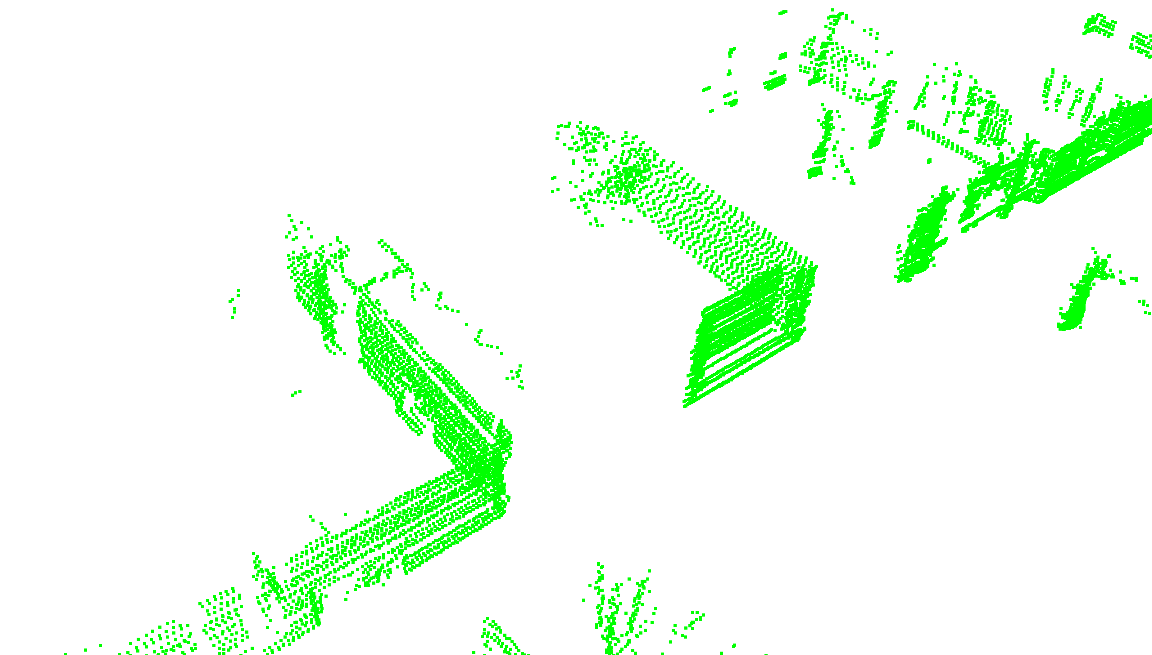
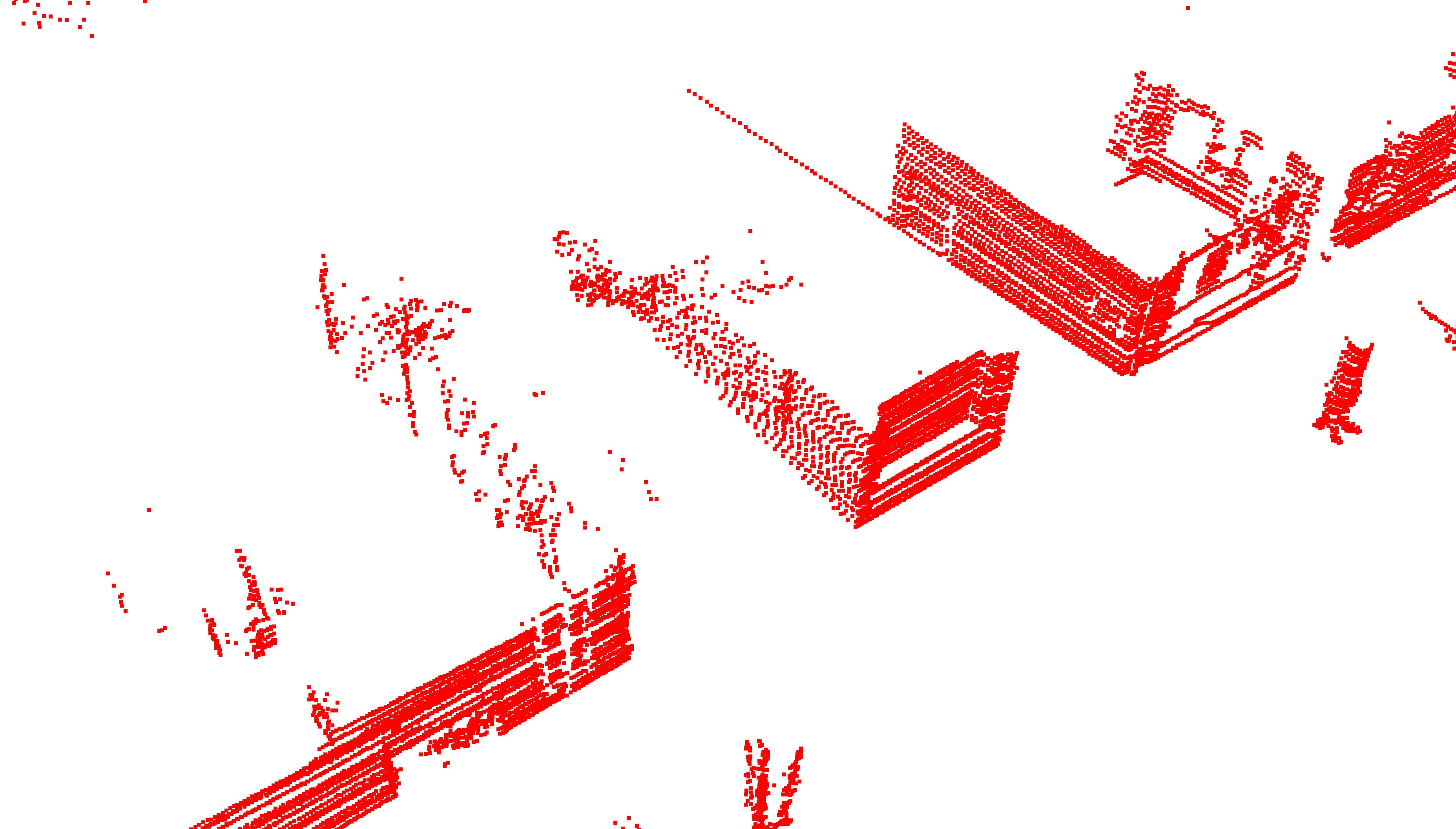
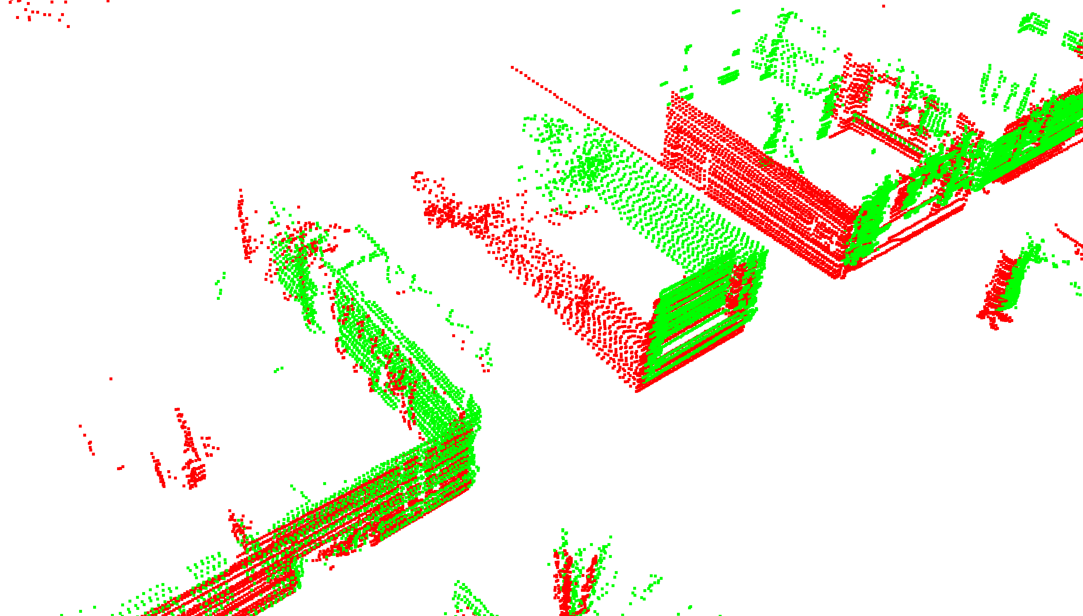
The single most important building block of 3D perception-enabled applications is registration, the process of aligning two frames of point cloud data to form a globally consistent view of the scene. Fig. 1 illustrates the registration of two point cloud frames. Augmented Reality applications align a sequence of frames to form a complete 3D model of the environment so as to place virtual objects. Similarly, a mobile robot estimates its real-time position and orientation (a.k.a., odometry) by aligning two consecutive frames, which provides the translational and rotational transformations. As these applications are increasingly deployed in embedded systems with limited performance and power budgets, this paper takes a first step toward enabling real-time, low-power 3D data registration.

We present Tigris, a software-hardware system specialized for 3D point cloud registration. Tigris achieves high efficiency not only by the specialized datapaths and control logics that mitigate common inefficiencies in general-purpose processors, but also by a combination of acceleration techniques that exploit unique characteristics of point cloud registration. In particular, Tigris identifies and exploits different forms of parallelism, captures unique data reuse patterns while reducing the overall compute demand. Critically, we enable these techniques by co-designing the data structure, algorithm, and the accelerator architecture.

We start by understanding the performance characteristics of point cloud registration and identifying the acceleration opportunities. The central challenge, however, is that point cloud registration exposes a large design space with many parameters that are often collectively co-optimized given a particular design target. In order to obtain general conclusions without overly specializing for one particular design point, we first construct a configurable registration pipeline, which let us perform a thorough design space exploration. Surprisingly, although different design points differ significantly in registration accuracy and compute-efficiency, KD-tree search is the single most dominant kernel across all design points, constituting over 50% of the registration time, and thus presents itself as a lucrative specialization target.

KD-tree search, however, is inherently sequential due to the recursive tree traversal. To enable effective hardware acceleration, we propose a parallel KD-tree search algorithm to introduce fine-grained parallelism that are amenable to hardware acceleration. The algorithm builds on top of the two-stage KD-tree data structure, a variant of KD-tree that provides high degrees of parallelism by balancing recursive search with brute-force search. However, two-stage KD-tree necessarily introduces lots of redundant computations in increasing parallelism. To mitigate the redundancies, we observe that point cloud registration is resilient to imprecisions introduced in KD-tree search due to the noisy nature of point cloud data. Our algorithm incorporates an approximate KD-tree search procedure that reduces workload while presenting massive parallelism to the hardware.

The new data structure and algorithm in conjunction uniquely expose two forms of parallelism in KD-tree search: query-level parallelism (QLP) and node-level parallelism (NLP). The key design principle of the hardware accelerator is to exploit the two forms of parallelism with proper architectural mechanisms. Specifically, the accelerator incorporates parallel processing elements (PE) to exploit the QLP while applying pipelining to exploit the NLP within a query. While parallel PEs and pipelining are well-established techniques, effectively applying them in KD-tree search requires us to design a set of architectural optimizations that leverage compute and data access patterns specific to KD-tree search.

We evaluate Tigris over a general-purpose system consisting of an Intel Xeon Silver 4110 CPU and an Nvidia RTX 2080 Ti GPU. We show that Tigris achieves 77.2$\times$ speedup and 7.4$\times$ power reduction in KD-tree search compared to the GPU, which translates to 41.7% speedup and 3.0$\times$ power reduction for the end-to-end registration.

To our best knowledge, this is the first paper focusing on architecture and system specializations for point cloud processing. In summary, we make the following contributions:

• We identify that KD-tree search is inherently a performance bottleneck in point cloud registration by carefully navigating the algorithmic and parametric design space of registration.

• We demonstrate that point cloud registration is tolerant to errors introduced in KD-tree search.

• We propose an acceleration-amenable KD-tree search algorithm. Building on top of a novel two-stage KD-tree data structure, the algorithm exposes massive parallelism to the hardware while reducing the compute.

• We co-design an accelerator architecture with the search algorithm. The accelerator incorporates a set of architectural optimizations that are specific to KD-tree search to effectively exploit different forms of parallelism.

The rest of the paper is organized as follows. Sec. 2 introduces the necessary background of point cloud processing. Sec. 3 performs extensive algorithmic design space exploration to identify that KD-tree search is the performance bottleneck of point cloud registration. Sec. 4 presents an acceleration-amenable KD-tree data structure and search algorithm, and Sec. 5 describes the corresponding Tigris accelerator architecture. Sec. 6 presents the experimental methodology and evaluation results. Sec. 7 puts Tigris in the broad context of related work, and Sec. 8 concludes the paper.

2. Background

This section first introduces point cloud data (Sec. 2.1). We then describe point cloud registration, a key task in many application domains that operate on point cloud data (Sec. 2.2).

2.1. Point Cloud Data

Point cloud is a collection of points in a given 3D Cartesian coordinate system. Each point in the point cloud represents the $<x,y,z>$ coordinates of a particular point in the 3D space. Point cloud directly preserves the 3D geometric information of a scene and the spatial relationship between objects of interest, avoiding the need to estimate such information from 2D images. The proliferation of 3D sensors and the emerging interests in 3D geometry-based applications such as robotics lead to massively increased use of 3D data, of which point cloud is the de-facto representation (Aldoma et al., 2012).

Point cloud data is obtained through 3D sensors, ranging from conventional stereo (Lucas et al., 1981) and structured-light cameras (Rocchini et al., 2001) that estimate the scene 3D geometry through computational methods to active sensors such as LiDAR (Schwarz, 2010) that operate on the ”time-of-flight” principles (Gokturk et al., 2004). While using different mechanisms, different sensors eventually produce the same point cloud data structure. Our paper focuses on the fundamental point cloud processing algorithms, and is independent of how the point cloud data is obtained.

2.2. Point Cloud Registration

A key building block in virtually all point cloud-based applications is registration, a process that finds the 4$\times$4 transformation matrix that aligns two point cloud frames to form a globally consistent point cloud. More specifically, given a source point cloud frame $\mathbf{S}$ and a target point cloud frame $\mathbf{T}$, the goal of registration is to estimate a transformation matrix $\mathbf{M}$, which transforms $\mathbf{S}$ to $\mathbf{S^{\prime}}$ in a way that minimizes the Euclidean distance (i.e., error) between $\mathbf{S^{\prime}}$ and $\mathbf{T}$. $\mathbf{S^{\prime}}$ is transformed from $\mathbf{S}$ by applying the transformation matrix $\mathbf{M}$ to every point $X$ in $\mathbf{S}$ to a point $X^{\prime}$ in $\mathbf{S^{\prime}}$:

(1) $$X^{{}^{\prime}}_{4\times 1}=\mathbf{M}X_{4\times 1}=\begin{bmatrix}R_{3\times 3}&T_{3\times 1}\\ 0_{1\times 3}&1\end{bmatrix}_{4\times 4}X_{4\times 1}$$

where $X=[x,y,z,1]^{T}$ and $X^{{}^{\prime}}=[x^{{}^{\prime}},y^{{}^{\prime}},z^{{}^{\prime}},1]^{T}$ are the homogeneous coordinates of $X$ and $X^{\prime}$, respectively. The 4$\times$4 transformation matrix $\mathbf{M}$ consists of a 3$\times$3 rotation matrix $\mathbf{R}$ and a 3$\times$1 translation matrix $\mathbf{T}$, representing all six degrees of freedom.

Significance of Registration

Point cloud registration is a key primitive that finds itself in many application domains.

In many cases point cloud registration is the end-to-end machine perception applications such as odometry and mapping. For instance, an autonomous navigation system could capture two consecutive frames $\mathbf{F}_{t}$ and $\mathbf{F}_{t+1}$ in time, and by registering $\mathbf{F}_{t+1}$ against $\mathbf{F}_{t}$ and obtaining the transformation matrix, the navigation system could estimate its own trajectory (rotation and translation) over time, a process known as odometry or ego-motion estimation (Irani et al., 1997; Zhang and Singh, 2015). Similarly, registration is key to 3D reconstruction (Vosselman et al., 2001), where a set of frames are aligned against one another and merged together to form a global point cloud of the scene. In other cases point cloud registration is part of the application pipeline to collaborate with other modalities such as camera (e.g., SLAM uses both visual data and point cloud) (Zhang and Singh, 2015; Park et al., 2017b).

This paper focuses on improving the efficiency of the core registration operation while being independent of how the high-level applications make use of the registration results.

Fig. 2. The general point cloud registration pipeline, which consists of an initial estimation phase and a fine-tuning phase. The pipeline exposes two kinds of design knobs for accuracy-performance trade-off analysis: algorithmic and parametric choices. Shaded stages make heavy use of KD-tree search, the single-most dominant kernel in all design points.

3. Performance Characterizations

Table 1. Algorithmic and parametric choices and of a general point cloud registration pipeline.

	Initial Estimation					Fine-Tuning
Stages	Normal Estimation	Key-point Detection	Descriptor Calculation	KPCE	Rejection	RPCE	Transformation Estimation
Algorithm Choices	PlaneSVD(Klasing et al., 2009) AreaWeighted(Klasing et al., 2009) DNN(Wang et al., 2015)	SIFT(Lowe, 2004; Scovanner et al., 2007) NARF(Steder et al., 2011) HARRIS(Harris et al., 1988; Sipiran and Bustos, 2011)	FPFH(Rusu et al., 2009) SHOT(Tombari et al., 2010) 3DSC(Frome et al., 2004)	-	Thresholding RANSAC(Fischler and Bolles, 1981)	Normal-shooting Projection(Blais and Levine, 1995)	Error metric(Rusinkiewicz and Levoy, 2001) Solver(Rusinkiewicz and Levoy, 2001)
Key Parameters	Search radius	Scale Range	Search radius	Reciprocity	Distance threshold Ratio threshold	# of neighbors Reciprocity	Convergence criteria

This section characterizes the performance of point cloud registration through a configurable registration pipeline design that exposes a large accuracy-performance trade-off space (Sec. 3.1). Through an exhaustive exploration of the design space covering both algorithmic and parametric choices, we find that different design points share the same performance bottleneck of KD-tree search, which is thus an ideal acceleration candidate (Sec. 3.2). We make the pipeline implementation publicly available at https://github.com/horizon-research/pointcloud-pipeline.

3.1. Point Cloud Registration Pipeline

Existing implementations of point cloud registration make different trade-offs between accuracy and performance. Intuitively, achieving a higher registration accuracy increases the workload, and vice versa. Our goal in this paper, however, is not to overly specialize for one particular implementation. Rather, we hope to derive general-purpose solutions that benefit different design points.

In order to obtain generally applicable conclusions, a key observation is that different registration implementations, while making different design decisions, all share a similar pipeline substrate. This allows us to construct a general-purpose pipeline with configurable knobs that cover different implementation instances. Critically, our pipeline exposes two kinds of design knobs for tuning: algorithmic choices and parametric choices within a particular algorithm.

At the high-level, our pipeline adopts a common two-phase design consisting of an initial estimation phase and a fine-tuning phase (Zhang and Singh, 2014; Huang et al., 2018). The first phase performs an initial estimation of the transformation matrix, which is then fine-tuned in the second phase until the accuracy converges. The rationale behind the two-phase design is that the fine-tuning phase usually uses an iterative solver to minimize the global registration error; the solver could easily be trapped at local minima if poorly initialized. A carefully designed initial estimation phase would thus significantly improve the efficiency and accuracy of fine-tuning. Fig. 2 illustrates the high-level architecture of the pipeline, and Tbl. 1 shows the different algorithmic and parametric knobs exposed by the pipeline.

The goal of the initial estimation phase is to calculate an initial transformation matrix by matching a set of salient points from the source point cloud to a set of salient points in the target cloud, similar to image registration (Zitova and Flusser, 2003), but in the 3D space.

(a) Translational error vs. time.

(b) Rotational error vs. time.

Fig. 3. Quantifying the accuracy-performance tradeoff. We annotate Pareto-optimal design points in both design spaces. Execution time is normalized to $1500\text{\,}\mathrm{ms}$.

1. Normal Estimation

   The front-end first calculates the surface normal of all points. A point’s normal is a 3D vector perpendicular to the tangent plane at the point. Normals are important metadata that will be used in later stages to calculate feature descriptors and to estimate correspondences.

2. Key-Point Detection

   This stage selects key-points which contains representative information, from both the target and source point clouds. Operating on the key-points rather than all the points improves the compute-efficiency of the front-end. We explore different feature extraction algorithms such as NARF (Steder et al., 2011) and SIFT (Lowe, 2004; Scovanner et al., 2007), as well as feature-specific parameters such as the scale of SIFT feature and the range of NARF feature.

3. Feature Descriptor Calculation

   This stage computes the feature descriptor of each key-point. A point’s feature descriptor is a high-dimensional representation that encodes neighborhood information of the point and therefore provides richer information for registration. Essentially, this stage converts the original 3D point space to a high-dimensional feature space. The dimension of the feature space depends on the specific feature descriptor being used. We explore different descriptors, including FPFH (Rusu et al., 2009) and SHOT (Tombari et al., 2010), as well as key algorithmic parameters such as the search radius when calculating the descriptors.

4. Key-Point Correspondence Estimation (KPCE)

   This stage establishes correspondences between the key-points in the source and the target point cloud frames using feature descriptors. Specifically, KPCE establishes the correspondence between a point $\mathbf{s}$ in the source frame and a point $\mathbf{t}$ in the target frame if $\mathbf{t}$’s feature is the nearest neighbor of $\mathbf{s}$’ feature in the feature space generated in the previous stage. We explore whether or not reciprocal search is performed.

5. Correspondence Rejection

   The final stage of the front-end removes incorrect correspondences produced by the previous stage, and generates a set of correct key-point correspondences, from which the initial transformation matrix $\mathbf{M}$ is estimated. We explore different correspondence rejection algorithms include the classic RANSAC algorithm (Fischler and Bolles, 1981) and ones that simply threshold the distance.

The initial transformation matrix $\mathbf{M}$ allows all points in the source point cloud $\mathbf{S}$ to be transformed to form a new point cloud $\mathbf{S^{\prime}}$. The fine-tuning phase then estimates the transformation matrix between $\mathbf{S^{\prime}}$ and the target point cloud $\mathbf{T}$, effectively refining the initial result. The fine-tuning phase uses the popular Iterative Closest Point (Besl and McKay, 1992; Chen and Medioni, 1992) framework, iterating between two stages:

1. Raw-Point Correspondence Estimation (RPCE)

   This stage establishes correspondences between all points from the source point cloud $\mathbf{S^{\prime}}$ and the target point cloud $\mathbf{T}$. For every point in $\mathbf{S^{\prime}}$, RPCE finds its nearest neighbor in $\mathbf{T}$. Different from KPCE, RPCE searches in the original 3D point space.

2. Transformation Estimation

   This stage formulates an error measure between every pair of corresponding points identified previously, and minimizes the error using an optimization solver, which produces the transformation matrix $\mathbf{M^{\prime}}$ between $\mathbf{S^{\prime}}$ and $\mathbf{T}$, and transforms $\mathbf{S^{\prime}}$ into $\mathbf{S^{\prime\prime}}$. $\mathbf{S^{\prime\prime}}$ then becomes the new source point cloud, and is fed back to the RPCE stage. We explore different error formulations (e.g., mean square point-to-point (Johnson and Kang, 1999) or point-to-plane error (Chen and Medioni, 1992)) and different solvers including the Singular Value Decomposition (Golub and Reinsch, 1971) and the Levenberg-Marquardt algorithm (Moré, 1978). Another key parameter that we explore is the convergence criteria, which determines the termination of ICP, and thus impacts both the accuracy and compute time.

(a) Distribution across the seven key stages (Fig. 2).

(b) Distribution between KD-tree search and other operations.

Fig. 4. Time distribution of point cloud registration of the eight Pareto-optimal design points (denoted as DP$i$) obtained from the design spaces in Fig. 3a and Fig. 3b.

3.2. Performance Bottleneck Analysis

(a) Canonical KD-tree data structure.

(b) Two-stage KD-tree data structure.

Fig. 5. Comparison between the canonical and the two-stage KD-tree data structures. Shaded nodes are visited during the search while the rest of the nodes are pruned. The top-tree in the two-staged data structure is exactly the same as the corresponding portion in the classic data structure. Each leaf node in the top-tree organizes its children as an unordered set rather than a sub-tree to enable exhaustive search. While exposing parallelism, the two-stage data structure requires visiting more nodes: nine nodes as opposed to six nodes required by the classic data structure in this example.

Design Space Exploration

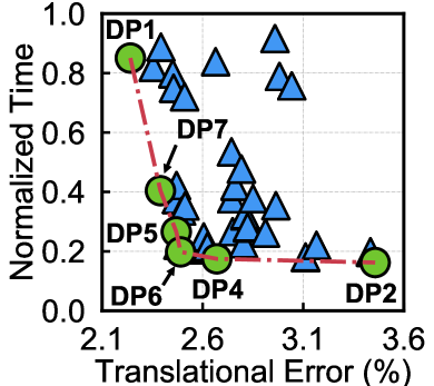
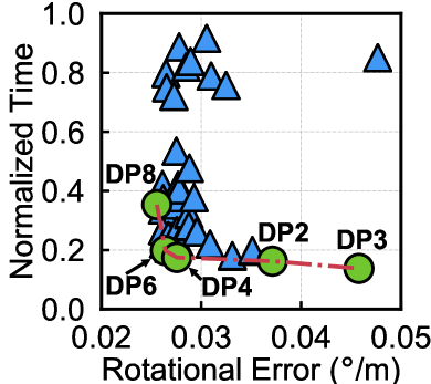
Using the configurable pipeline, this section performs a design space exploration (DSE) to identify representative design points, on which we then study the performance bottlenecks. The design space is specified by the different algorithmic choices and parameter values described in Tbl. 1. We use the widely-adopted KITTI dataset (Geiger et al., 2012) and perform the experiments on a Xeon 4110 processor (see Sec. 6.1 for detailed experimental setup). Fig. 3a shows how different design points trade translation error for execution time, and Fig. 3b shows the trade-off between rotational error and execution time. The DSE results confirm the vast trade-offs space exposed by our configurable pipeline. More importantly, we are able to identify the Pareto-optimal frontier in each design space as annotated both in  Fig. 3a and  Fig. 3b. To draw meaningful conclusions, we now focus on analyzing the Pareto-optimal design points from both design spaces.

Performance Bottleneck

Our goal is to identify “universal” performance bottlenecks that, if accelerated, would lead to speed improvements on a wide range of design points rather than being overly tied to a particular design point.

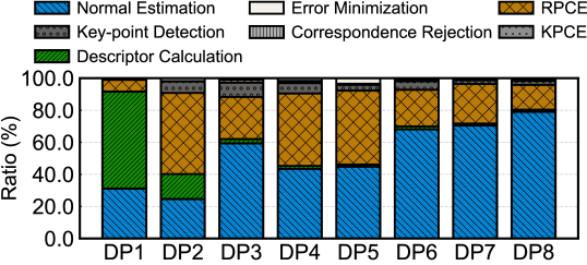
To that end, we first examine the per-stage performance of the pipeline. Fig. 4a shows the registration time distribution across the seven key stages as described in Fig. 2 for the eight Pareto-optimal design points (DP). Normal Estimation, Descriptor Calculation, and RPCE are three dominating stages, constituting to over 90% of the total time. However, there is no single dominant stage that is consistent across different design points. For instance, while the Normal Estimation stage contributes to about 80% of the execution time in DP8 and thus is an ideal acceleration target, it contributes to less than 30% of the execution time in DP1 and DP2. The diversity of stage-wise time distribution indicates that accelerating any single stage would not yield a general solution.

Looking into the operations within each stage, however, we find that Normal Estimation, Descriptor Calculation, and RPCE all make heavy use of neighbor search. For instance, to calculate the surface normal for a given point in the Normal Estimation stage, one must identify the neighbors of the given point in order to form a surface, with which the normal is calculated. Similarly, the very definition of “correspondence” in the RPCE stage requires identifying the nearest neighbor of a given point. In particular, KD-tree is arguably the most efficient data structure that is widely used in neighbor search, providing an average time complexity of $O(\log{}n)$ (Bentley, 1975; Finkel et al., 1977). The majority of the point cloud registration implementations use KD-tree for neighbor search (Greenspan and Yurick, 2003; Li et al., 2016; Wang et al., 2017; Shi et al., 2016). We thus equate KD-tree search with neighbor search in the rest of the paper.

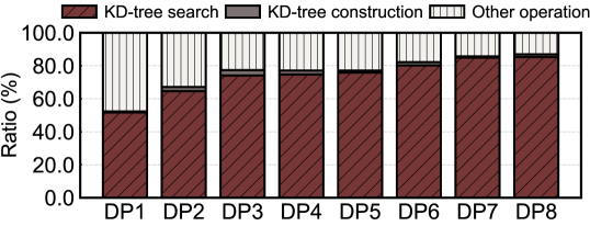
As a result of the inherently algorithmic requirement of different pipeline stages, KD-tree search is a key operation that dominates the registration time across different DPs. Fig. 4b shows that the KD-tree search operation consistently contributes to 50% - 85% of the total time in all the design points. Accelerating KD-tree would thus be a key performance optimization that is generally applicable to different point cloud registration implementations.

4. Acceleration-Amenable KD-Tree Data Structure and Algorithm

KD-tree search is inherently sequential as it requires tree traversal (Bentley, 1975). To enable hardware acceleration, we propose a mechanism that exposes massive parallelism in KD-tree search while reducing the total compute – at the cost of negligible end-to-end accuracy loss. The key is to co-design the KD-tree data structure with a new approximate search algorithm. This section first describes a parallelism-exposing KD-tree data structure (Sec. 4.1). We then quantify the error-tolerating nature of KD-tree search (Sec. 4.2), and describe our new search algorithm (Sec. 4.3).

4.1. Two-Stage KD-Tree Data Structure

We first briefly describe the classic KD-tree data structure and its associated search algorithm. We then describe the two-stage KD-tree data structure, which exposes higher degrees of parallelism during search while introducing redundant work.

Canonical KD-Tree

A KD-tree is a data structure that organizes points in a k-dimensional space in a binary search tree to enable efficient search (Bentley, 1975). Each tree node stores a k-dimensional point. The point on each non-leaf node implicitly generates a splitting hyperplane that divides the space into two half-spaces. Points that lie in the left half-space are stored in the left sub-tree, and points that lie in the right half-space are stored in the right sub-tree. Essentially, each non-leaf node corresponds to a bounding box in the k-dimensional space that encapsulates all the nodes in its sub-tree. Usually the median point is used to generate the splitting plane such that the resulting KD-tree is a balance tree.

Point cloud registration mainly involves two kinds of search: radius search and Nearest Neighbor (NN) search. Given a query, which itself is also a point in the k-dimensional space, the former returns all the points in the point cloud that are within the given radius to the query point, and the latter returns the nearest neighbor to the query point. Without losing generality, we use NN search to drive the explanation.

The KD-tree search algorithm starts from the root node, and recursively traverses the tree using the query point. As the algorithm visits a node, it checks whether the node should be added to the return results by comparing against the current nearest distance $d$. The algorithm then further searches the left and right sub-tree of the current node. Critically, if the bounding box of either sub-tree does not intersect with the hypersphere surrounding the query point with the $d$, the entire sub-tree could be skipped because all of its nodes are guaranteed to lie outside of $d$. This is a key technique called pruning that enables efficient search in KD-tree. Fig. 5a shows a simple KD-tree example, where the shaded points are visited during the search while the rest of the points are pruned.

While pruning reduces redundant computations by skipping unnecessary nodes, it serializes the search: every time the algorithm visits a node, it might obtain a new current nearest distance, which allows for pruning more nodes later.

Two-Stage KD-Tree

To balance parallelism and redundancies, we use a slight variant of the canonical KD-tree data structure called two-stage KD-tree. Fig. 5b shows the two-stage KD-tree organization of the same points stored in the canonical KD-tree (Fig. 5a). The two-stage KD-tree is split into two halves. The top half, which we call the top-tree, is a tree with height $h_{top}$. The top-tree is exactly the same as the first $h_{top}$ levels of the classic KD-tree. Each top-tree leaf node organizes its children as an unordered set as opposed to a sub-tree as in the canonical data structure.

Since the leaf nodes of the top-tree organize their children as unordered sets, different child nodes of a leaf node can be searched in parallel. Essentially, the two-stage KD-tree enables exhaustive searches in certain sub-trees. In the extreme case where $h_{top}$ is 0, searching in the two-stage KD-tree is equivalent to exhaustively searching all the points. Fundamentally, the two-stage KD-tree introduces more parallelism at the cost of higher redundancies compared to the canonical KD-tree data structure. In the example of Fig. 5, searching in the two-stage data structure visits nine nodes, three when traversing the top-tree and six when exhaustively searching a leaf node of the top-tree, as opposed to six nodes required by the classic data structure.

(a) Redundancy ratio.

(b) Total number of nodes visited.

Fig. 6. The two-stage KD-tree introduces redundant visits to nodes. Redundancy is quantified as the ratio between the number of nodes visited in the two-stage KD-tree and that in the classic KD-tree. Redundancy increases as the leaf-set size grows. The leaf-set size is defined as the number of children in the leaf node’s unordered set.

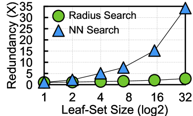
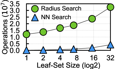
Intuitively, a shorter top-tree exposes more parallelism but also introduces more redundancies. Using the KITTI Odometry Dataset (see Sec. 6.1 for the detailed experimental setup), Fig. 6a shows how the redundancy introduced by the exhaustive searches varies with the leaf-set size for both radius search and NN search. The redundancy is quantified as the ratio between the number of nodes visited in the two-stage KD-tree and that in the classic KD-tree. The leaf-set size is defined as the number of children in the leaf node’s unordered set. The classic KD-tree has a leaf-size one, and the two-stage KD-tree in Fig. 5b has a leaf-set size six.

As the leaf-set size increases, the top-tree height decreases and more exhaustive searches occur. Thus, the redundancy increases. With a leaf-set size of 32, the two-stage KD-tree introduces about 35$\times$ redundant node visits for NN search and about 3$\times$ for radius search. The redundancy grows much faster for the NN search than for the radius search because the NN search benefits more from pruning than the radius search, and thus suffers more from exhaustive searches. While the redundancy introduced to radius search seems lower than NN search, the sheer number of nodes that radius search has to visit is much greater than NN search as shown in Fig. 6b, which shows the absolute number of nodes visited as the leaf-set size increases. Thus, the redundancies introduced by the two-stage KD-tree is significant for radius search as well.

4.2. Quantifying the Error-Tolerance

(a) Sensitivity of translational error as the NN search returns the $k^{th}$ nearest neighbor instead of the nearest neighbor.

(b) Sensitivity of translational error as the radius search returns points between ¡$r1,r2$¿ rather than within $r$ ($r$ = $60\text{\,}\mathrm{cm}$ here).

Fig. 7. Registration error ($y$-axis) varies as the degree of error ($x$-axis) changes. The error is robust against inexactness of KD-tree search when searching dense points (NE and RPCE), but is sensitive when searching sparse points (KPCE).

While the two-stage KD-tree data structure exposes more parallelism, it also introduces lots of redundancies to the search on leaf nodes. To mitigate the redundancies, our key observation is that KD-tree search does not have to be exact because the entire point cloud registration pipeline is error-tolerant. By performing inexact searches on the two-stage KD-tree, we could reduce the amount of computations while retaining parallelism. This section quantitatively demonstrates the error resilience while leaving the mechanisms to exploit the resilience to the next section.

There are two reasons that point cloud registration is resilient to inexact KD-tree search. First, acquiring point cloud data is inherently an approximation process due to the sensor noise. The movement of the sensor during acquisition further adds uncertainties to data acquisition. Second, the registration algorithm strives to minimize the global error, where local inexactness would be compensated at the global scale.

Error Injection

To understand the impact of inexact KD-tree search on the registration accuracy, we manually inject errors into the KD-tree search, and quantify how the end-to-end registration accuracy varies with the KD-tree search accuracy. Specifically, we inject errors into the nearest neighbor (NN) search by replacing the return result, i.e., the nearest neighbor to the query, with a point that is the $k^{th}$ nearest neighbor to the query point. Similarly, we inject errors into radius search by replacing the return results, i.e, points that lie within a sphere delineated by the radius $r$, with points that lie within a spherical shell delineated by two radiuses $r1$ and $r2$, where $r1<r<r2$. The parameters $k$ and $<r1$, $r2>$ control the degrees of error injected into the radius search and the NN search on KD-tree, respectively.

Input: QuerySet $\mathbb{Q}$; LeafNode $LF$; Threshold $thd$.

Result: Search result $q.res$ for all $q$ in $\mathbb{Q}$.

for $q$ in $\mathbb{Q}$ do

       if $LF.leaders.size()$ then

             // Find the closest leader for $q$

             $closestLeader=getMinDist(q,LF.leaders)$

             if $dist(q,closestLeader)<thd$ then

                   // Approximate path: search in the results of $closestLeader$

                   $q.res=bf{\text{-}}search(q,closestLeader.res)$

                   continue;

                  

             end if

            

       end if

      // Precise path: search in all the children of the leaf node $LF$

       $q.res=bf{\text{-}}search(q,LF.children)$

       $LF.leaders.pushback(q)$

      

end for

Algorithm 1 Approximate KD-Tree Search.

Error Tolerance

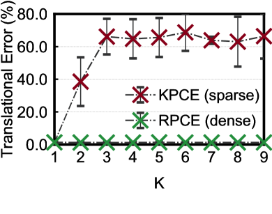
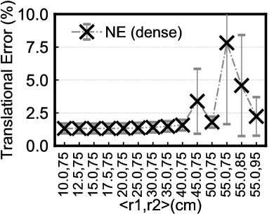
While multiple stages make use of KD-tree search, we mainly inject errors into two stages: Normal Estimation (NE) and Raw-Point Correspondence Estimation (RPCE), both contributing heavily to the total execution time (Fig. 4a). The former uses radius search and the latter uses NN search. Fig. 7a and Fig. 7b show how the end-to-end registration error varies with different degrees of error injected into RPCE and NE, respectively. Due to space limit, we show only the translational error; the trend on rotational error is similar. Error bars denote the standard deviation of all the frames’ errors in one sequence.

We find that the registration error is statistically robust to errors introduced in both the radius search and NN search, indicating the potential of relaxing KD-tree search accuracy. For instance, the registration error is virtually the same if the radius search returns the points between $<30,75>$ compared to the precise search that returns points within $r=65$.

Critically, not all instances of KD-tree search are equally amenable to approximation. While the NE stage and the RPCE stage both operate on dense points, we find that errors introduced in KD-tree search that operates on sparse data are detrimental to registration accuracy. For instance, the Key-Point Correspondence Estimation (KPCE) stage operates on sparse (feature) data. Fig. 7a overlays how the registration accuracy varies with the error degree introduced in the KPCE stage. Returning just the second nearest neighbor leads to about 40% registration accuracy loss.

Overall, we find that KD-tree searches that operate on dense points are amenable to approximation, and thus provide an opportunity to greatly reduce the amount of computations in the KD-tree search. We particular focus on the NE and RPCE stages as they dominate the end-to-end performance.

4.3. Approximate KD-Tree Search

Motivated by the error resilience of the point cloud registration pipeline, we propose an approximate KD-tree search algorithm that reduces computation overheads with little accuracy loss. Our key observation is that queries arriving at the same leaf node in the top-tree are close to each other as they fall into the same 3D partition. Therefore, it is likely that their search results are similar.

Leveraging this insight, our idea is to split queries arriving at the same leaf node into a leaders group and a followers group. Queries in the leaders group perform an exhaustive search in the leaf node’s children as usual, while queries in the followers group search in only the return results of the closest leader. To dynamically adjust the leaders group, we introduce a discriminator $thd$; if the distance between a query point and the closest leader is greater than $thd$, the query point is added to the leaders group. Algo. 1 shows the pseudo-code of the algorithm.

This algorithm relies on an efficiency trade-off: it allows a follower query to search in a much smaller space, i.e., its closest leader’s neighboring points as opposed to all the children of the leaf node, while incurring the cost to find the closest leader. Assuming that one leaf node has $N$ children points; there are $L$ points in the leaders group, and the returned neighbors of a leader consists of $R$ points. A follower query would compare against $L+R$ points, which should be much smaller than $N$ for the algorithm to succeed. This first-order cost model is used to understand the performance gains in Sec. 6.3.

5. KD-Tree Accelerator Design

Fig. 8. The Tigris accelerator architecture overview. The front-end (FE) consists of a set of recursion units (RU) that process queries in the top-tree. The back-end (BE) consists of a set of search units (SU) that process queries by exhaustively searching children in the leaf nodes. Queries are distributed from the FE to the BE buffers, and the BE reinserts queries to the FE query queue. The global buffer maintains all the necessary metadata.

This section describes the accelerator design. We first provide an overview of the architecture (Sec. 5.1). We then describe its two key components: the front-end (Sec. 5.2) and the back-end (Sec. 5.3).

Fig. 9. Recursion unit (RU) pipeline overview. Each RU recursively traverses the top-tree in a DFS manner for one query at a time. The traversal status is maintained by a stack, introducing data dependencies between the PI and the RS stages. Node bypassing and forwarding eliminate the pipeline stalls.

5.1. Accelerator Overview

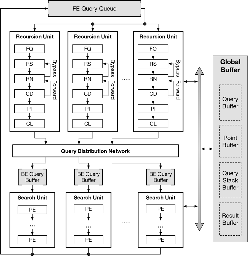
The new data structure and search algorithm expose two levels of parallelism. First, each query can be processed in parallel, both in searching the top-tree and in exhaustively searching leaf nodes. We call it query-level parallelism (QLP). Second, in the exhaustive search stage, different child nodes could be processed in parallel within each query. We call it node-level parallelism (NLP). The hardware architecture is designed to provide the mechanisms to support the two forms of parallelism while exploiting the data locality. Fig. 8 shows an overview of the accelerator.

The accelerator consists of a Front-End (FE) that is responsible for searching in the top-tree and a Back-End (BE) that is responsible for searching in the leaf nodes. The FE uses a set of Recursion Units (RU), each processing one query at a time, to exploit QLP in the top-tree. Each incoming query is first inserted into the FE Query Queue (FQQ), from which each RU deques a query to search in the top-tree. Once the top-tree search for a query is finished, the RU sends the query to the BE. The BE uses a set of Search Units (SU), each responsible for a set of leaf nodes. Queries coming from the FE are first inserted into an SU’s BE Query Buffer (BQB), from which the SU schedules the queries to execute. Each SU has a set of Processing Elements (PEs), exploiting both QLP and NLP.

Processing search queries requires a set of input and output metadata, which is stored in a global buffer. Specifically, the buffer is partitioned to hold the following metadata: (1) an Input Point Buffer that holds all the points in the point cloud, (2) a Query Buffer that holds all the query points, (3) a Result Buffer that holds the return results, and (4) a Query Stack Buffer that holds the recursion stacks for all the queries. We reserve the maximal number of stack entries for each query (i.e., the height of the top tree) in the buffer.

5.2. The Front-End: Recursion Unit

The FE processes queries in the top-tree. For each query, the FE recursively searches the top tree until a leaf node is reached, upon which time the query will be sent to BE. To exploit QLP, the FE consists of a set of RUs. Each RU independently processes a query popped from the FQQ.

While different RUs can exploit the QLP, processing within each query is sequential due to the inherent nature of depth-first search: the RU would have to finish the current node before deciding whether/how to proceed to the next node in the top-tree. The key challenge in the RU design is thus how to expose intra-query parallelism to improve performance. To that end, we start from a simple hardware design, and gradually introduce architectural optimizations that exploit pipelining.

Baseline Design

Processing a query in the top-tree requires iteratively traversing the top-tree in a DFS manner. We use a stack to maintain the traversal status. Each iteration processes the node at the top of the stack, and pushes the two children nodes back to the stack in the end. Therefore, processing a query consists of the following six stages:

• FQ: fetch the query point $Q$ from the FQQ and obtain the query information, including the address of the query stack in the global buffer;

• RS: read the top of the stack (TOS) from the query stack; the TOS structure contains the address of the next top-tree node $N$ to be visited;

• RN: read the data of $N$ from the global buffer;

• CD: calculate the distance $Dist$ between $Q$ and $N$;

• PI: push the two child nodes to the stack, and use $Dist$ to decide whether to insert $N$ to the Result Buffer;

• CL: issue the query to the BE if a leaf node is reached.

The baseline six-stage RU design is illustrated in Fig. 9. The first stage prepares the query data and is required only at the beginning of the query, while the rest five stages are required for each iteration during the query processing. Critically, there is a data dependency between the PI stage that pushes data to the stack and the RS stage that popes data from the stack. This dependency stalls the pipeline for 3 cycles between searching consecutive top-tree nodes. We propose two architectural optimizations that eliminate the stalls and improve performance.

Fig. 10. Search unit (SU) overview. Each SU has a set of processing elements (PE) operating in the SIMD fashion. The PEs are organized as a 1D systolic array to improve data distribution efficiency. The SU adopts a “ query-stationary” data-flow where each query is pinned at a PE and the search nodes are streamed through the PEs (i.e., reused by different queries).

Node Forwarding

We observe that the PI stage pushes the current node’s two child nodes, $N1$ and $N2$, to the stack; whichever child node gets pushed later will necessarily be popped in the next iteration. Thus, if $N1$ gets pushed first, the PI stage could then directly forward $N2$ to the RN stage, eliminating one stall cycle. To completely remove stalls, we observe that the logic to decide which child node gets pushed first could be determined early in the CD stage rather than waiting until the PI stage. Moving that decision logic earlier to the CD stage completely eliminates stalls.

Node Bypassing

Forwarding eliminates stalls when a node gets to the PI stage. Node bypassing aims at finishing a node early in the pipeline, allowing the next node to start immediately. Specifically, if a node is deemed to be prunable, its entire sub-tree could be skipped (Sec. 4.1). As a result, that node needs not go through the rest steps (i.e., bypassed). Bypassing pruned nodes is particularly significant in NN search when the top-tree is short. A short top-tree would allow the exhaustive search stage to obtain a tighter current nearest distance, exposing more pruned nodes.

To support bypassing, we augment a node’s metadata with the distance information, which gets decoded in the RN stage, which in turn generates the bypass signal to let the RS stage start the next node immediately.

5.3. The Back-End: Search Unit

Each query that arrives at the BE comes from a particular leaf node in the top-tree. The BE processes the query by exhaustively searching through the leaf node’s children, which we call a Node Set. The BE exhibits both QLP and NLP. To exploit QLP, the BE incorporates a set of PEs, each handling one query at a time. The Query Point Access logic fetches a query from the Query Buffer at the beginning of query processing, and stores the query point in a PE-local register. Fig. 10 shows the design of each PE.

Each PE exploits NLP within a query in a pipelined fashion. The PE datapath is pipelined into three stages, through which the nodes in the Node Set are streamed. Stage one reads a child node $N$ driven by the Search Node Access logic. Stage two computes the distance $Dist$ between the query point $Q$ and $N$. The final stage decides whether to insert $N$ into the Result Buffer depending on $Dist$. The pipeline is guaranteed to proceed with no stalls because there are no dependencies across different child nodes.

MQMN vs. MQSN

A naive BE design would allow each PE to handle any arbitrary query distributed from the FE to maximize the PE utilization. This design, however, leads to high memory bandwidth requirements because each PE would potentially have to read a different Node List. We call this design Multiple Query Multiple NodeSet (MQMN). The alternative is to force all the PEs to process queries from the same leaf node, which lowers memory bandwidth requirements as different PEs consume the same Node List. We call this design Multiple Query Single NodeSet (MQSN).

While MQSN is memory-efficient, the query issue logic would have to perform an associative search in the BE Query Buffer to find as many queries from the same leaf node as possible. This is key to ensure a high PE array utilization, which, however increases the design complexity and the pipeline cycle time.

Hierarchical MQSN

To enable a complexity-effective PE design while achieving high PE utilization, the BE groups the PEs into several groups, each responsible for only a set of leaf nodes. In this way, the issue logic has a much smaller scheduling window and has fewer PEs to keep occupied, increasing both the scheduling efficiency and the PE utilization.

We call each group a search unit (SU). More specifically, each SU has a set of PEs, a BE Query Buffer that holds queries that are sent to the SU from the FE, a query issue logic to issue queries to the PEs, and a set of address generation logic to access search nodes and query points. With this hierarchical design, we find that MQSN is able to achieve similar PE utilization as MQMN while being complexity-effective. We thus adopt the MQSN design, and will quantify its performance against MQMN later.

The associative search performed by the query issue logic uses the first query in the BQB as the search key, and search the remaining entries in the BQB. The search is done in groups of 32 queries in parallel, and terminates when we find enough queries for the PEs to operate on. The cost of the associative search is amortized across the execution of the found queries, which typically takes two orders of magnitude longer than the associative search.

We find that the overall performance is relatively insensitive to how exactly the leaf nodes are mapped to each SU. Thus, we use a simple policy that uses the low-order bits as the target SU ID. The Query Distribution Network sitting in-between the FE and BE is hard-wired with this logic.

Systolic PE Organization

To reduce the data distribution cost, we organize the different PEs in a SU as a 1D systolic array (Kung, 1982). Fig. 10 shows an example with two PEs, and the nodes in the same Node Set are streamed through the PEs to be reused by different queries. This dataflow is naturally “query stationary” as each query is pinned at a PE. Alternatively, the PEs could be organized as a set of SIMD lanes, requiring a data distribution fabric (e.g., bus) with support for multicasts to keep the PEs utilized (sim, 2018).

Approximate Search

Our SU design supports approximate search (Sec. 4.3), which allows a follower query to search in the return results of the leader queries instead of the leaf node’s Node Set. To that end, we augment the memory access logic with a Leader Check logic, which, when determines that the current query could be approximated by a leader, would drive the Search Node Access logic to fetch search nodes from the Result Buffer rather than from the Input Point Buffer. The actual check requires computing the distances between an incoming query and the existing leaders. We reuse the PEs in the SU for these computations.

The leader queries of each leaf node are stored in a local Leader Buffer, which we cap at 16 entries guided by the profiling results on the KITTI dataset (Geiger et al., 2012). The leader group stops growing after the buffer is full, which we find rare in our experiments, to simplify the hardware implementation. It is worth noting that capping the Leader Buffer improves accuracy because more queries will be searched exactly without relying on the leaders.

Node Cache

While the MQSN design significantly reduces the Node Set load traffic, loading from the Node Sets still contributes to over half of the total memory traffic. We observe that queries consecutively issued from the FE are likely from a small set of leaf nodes. We propose a cache design to capture the locality when loading the Node Sets to further reduce the memory traffic.

The node cache is organized as a set of entires, each containing the nodes in one Node Set. The nodes in each entry is organized as a FIFO queue because nodes in a Node Set are accessed sequentially. While there is a need to associatively search different entries to determine whether a particular Node Set is in the cache, the nodes within an entry could be accessed as a FIFO, greatly simplifying the hardware implementation.

6. Evaluation

We first describe the evaluation methodology (Sec. 6.1). We then analyze the area of the Tigris accelerator (Sec. 6.2). We then compare the performance and energy consumption of the accelerator over the baseline system for both the KD-tree search alone and the end-to-end pipeline (Sec. 6.3). We tease apart the contributions from different optimizations (Sec. 6.4), and analyze how the performance of Tigris is sensitive to different resource configurations (Sec. 6.5).

6.1. Experimental Methodology

Hardware Implementation

We synthesize, place, and route the accelerator datapath using Synposys and Cadence tools in a 16nm process technology, with memories generated using an SRAM compiler. Power is estimated using Synopsys PrimeTimePX by annotating the switching activity. The datapath is able to be clocked at 500 MHz. The DRAM energy is estimated using Micron’s DDR4 specification (Micron Technology, 2018) and power calculator (mic, 2019). We then use a cycle-accurate simulator parameterized with the synthesis and memory estimations to drive the performance and energy analysis.

Dataset

We evaluate Tigris on the widely-used KITTI Odometry dataset (Geiger et al., 2012). We use the first 11 sequences in the dataset that has ground truth. Each sequence consists of hundreds to thousands of point cloud frames. The point cloud in the KITTI dataset is obtained using the popular Velodyne HDL-64E LiDAR (Velodyne LiDAR, 2018), representative of today’s point cloud acquisition system. We report the average results across all the frames, unless noted otherwise.

Metrics

We evaluate Tigris in performance, energy, and accuracy. We show both the KD-tree time and the end-to-end registration time for all the frames in the entire sequence. The accuracy is measured using standard rotational and translational errors (Geiger et al., 2012).

Baseline

While the performance characterizations are performed on a CPU-based implementation (Sec. 3.2) as most of today’s point cloud registration pipelines are implemented on the CPU (Geiger et al., [n. d.]), for a fair evaluation we use a GPU/CUDA implementation of KD-tree search from the popular FLANN library (Muja and Lowe, 2014). KD-tree search on the GPU is about 8–20$\times$ faster than on the CPU.

We use a CPU-GPU setup as the baseline system. The KD-tree searches run on the GPU while all other operations run on the CPU. The CPU is a 32-core Xeon Silver 4110 Processor, and the GPU is an Nvidia GeForce RTX 2080 Ti. We use the widely-used Point Cloud Library (PCL) (Rusu and Cousins, 2011) to develop the registration pipelines, and integrate the FLANN’s implementation of KD-tree search. The GPU power is measured at 100 Hz using the nvidia-smi utility, and the CPU power is measured using the Intel RAPL energy counters (David et al., 2010) via directly reading the processor MSRs (xeo, 2018).

To demonstrate the generally applicability of Tigris, we evaluate it on two Pareto-optimal designs of the point cloud registration pipeline (Fig. 4 in Sec. 3.2): DP4 that optimizes for performance and DP7 that optimizes for accuracy.

6.2. Area Analysis

We configure the Tigris accelerator to have 64 RUs, 32 SUs, and 32 PEs per SU. We size the on-chip SRAM to accommodate about 130,000 points per frame, representative of the point cloud density acquired in the real-world. In particular, the Input Point Buffer and the Query Buffer are both sized at 1.5 MB; the Query Stack Buffer is sized at 1.2 MB, accommodating a maximal top-tree height of 18, sufficient for the KITTI dataset; the FE Query Queue is sized at 1.5 MB, and the BE Query Buffer is sized at 1 KB per SU, holding 128 BE queries at a time. The Node Cache is configured at 128 KB. Finally, the Result Buffer is set at 3 MB, which is double-buffered to interface with the DRAM to take the result write traffic off the critical path. Overall, the SRAM is estimated to take $8.38\text{\,}{\mathrm{mm}}^{2}$.

The datapath area of each RU and each SU’s PE is mostly dominated by the logic that computes the euclidean distance between two points using 32-bit floating point arithmetics. The total combinational logic occupies about $7.19\text{\,}{\mathrm{mm}}^{2}$. Overall, 53.8% of area is taken by SRAM and 46.2% is occupied by compute logic.

6.3. Performance and Power Comparisons

Speedup

Tigris achieves significant speedup in KD-tree search compared to the baseline. Using the accuracy-oriented design point DP7 as an example, Fig. 11a shows the KD-tree search speedup of the Tigris accelerator running both the original KD-tree (Acc-KD) and the two-stage KD-tree with a top-tree height of 10 (leaf-set size of about 128) (Acc-2SKD) compared to the GPU baseline that runs the original KD-tree, i.e., leaf-set size 1 (Base-KD). For comparison purposes, we also show the speedup of the GPU running the two-stage KD-tree with the same top-tree height 10 (Base-2SKD). Note that both Acc-KD and Acc-2SKD do not apply approximate search here, i.e., no accuracy loss.

(a) Accuracy-oriented DP7.

(b) Performance-oriented DP4.

Fig. 11. KD-tree search speedup and power reduction on two Pareto-optimal designs: DP7 is accuracy-oriented and DP4 is performance-oriented.

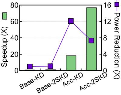
Acc-2SKD achieves 77.2$\times$ speedup in KD-tree search compared to Base-2SKD, which in turn is 28.3% faster than Base-KD. Acc-KD however, is “only” 18.7$\times$ faster than the Base-KD baseline. This is because using the original KD-tree, the accelerator’s performance is almost completely bottlenecked by the recursive search in the top-tree while the back-end SUs are almost always idle, leading to resource under-utilization. This confirms the need to co-design accelerator with the new data structure that exposes parallelism. Compared to the CPU implementation of KD-tree (not shown), Acc-2SKD achieves a speed up of 392.2$\times$.

The speedup on KD-tree search translates to significant end-to-end performance improvement. Specifically, Acc-2SKD reduces the overall registration time by 41.7% and 86.6% compared to the GPU baseline Base-KD and the CPU-only implementation, respectively.

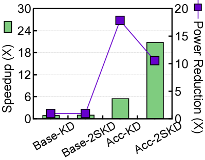
Tigris also achieves high speedups in the performance-oriented design point DP4. Fig. 11b shows the performance comparisons across different systems for DP4. Acc-2SKD achieves about 21.0$\times$ speedup compared to Base-2SKD on KD-tree search alone, which translates to about 13.6% end-to-end performance improvement. The speedup on the DP4 is lower than DP7 because in optimizing for performance DP4 uses tight search criteria that leads to much fewer exhaustive searches. For instance, the Normal Estimation stage in DP4 uses a radius of 0.30 while using a radius of 0.75 in DP7. A relaxed radius exposes more exhaustive searches, which could benefit from the SU design of Tigris. Overall, the performance improvements on two very different design points demonstrate the general applicability of Tigris.

Power Reductions

We overlay the power reductions on the right $y$-axis in Fig. 11a and Fig. 11b. Acc-2SKD achieves about 7$\times$ and 10.5$\times$ power reductions compared to Base-KD on KD-tree search for DP7 and DP4, respectively. The reduction along with the speedup further translates to significant energy savings (i.e., power-efficiency). For instance, Acc-2SKD reduces the energy consumption of Base-KD by a factor of 220.2 on DP4. Breaking down the energy consumption of DP4, the PE contributes to about 53.7% of the total energy consumption. The rest of energy is contributed by SRAM read(34.8%), SRAM write(8.0%), Leakage(3.3%), and DRAM read/write(0.2%). Over the end-to-end pipeline, Acc-2SKD achieves about a 3.0$\times$ power reduction compared to Base-KD.

The power consumption of Acc-KD is lower than Acc-2SKD, because Acc-KD does not expose exhaustive searches in the leaf nodes, and thus exclusively exercises the RUs while leaving the SUs idle. It trades lower power for lower performance. As a result, its overall energy consumption is about 2.5$\times$ higher than Acc-2SKD.

Approximate Search

We empirically choose 1.2 meters as the approximate threshold (Sec. 4.3) for the NN search, and use 40% of the original radius as the threshold in the radius search. Using these settings, the approximate search has no impact on translation errors, and increases the rotational error only by $0.05\text{\,}\mathrm{\SIUnitSymbolDegree}$/meter on DP4 and $0.0006\text{\,}\mathrm{\SIUnitSymbolDegree}$/meter on DP7.

Using DP7 as an example, the approximate KD-tree search achieves about 11.1$\times$ performance improvements over Acc-2SKD, translating to 7.5% end-to-end performance improvement. The improvement is a direct result of the compute reduction: the approximate algorithm reduces the number of nodes visited during search by 72.8%, to which NN search contributes 41.6% and radius search contributes 31.2%.

Fig. 12. The speedup and power reduction of architectural optimizations.

Fig. 13. The memory traffic distributions. Point cache alleviates Point buffer traffic.

6.4. Optimization Effects

Bypassing and Forwarding

In the RU design, bypassing allows pruned nodes to take an early exit from the pipeline, and forwarding allows the node that will soon be at the top of the query stack to start immediately. Both techniques help reduce pipeline stalls and improve the performance. Fig. 13 shows the speedup over Base-KD of three Acc-2SKD variants: without either technique (No-Opt), with just bypassing (Bypass), and with both bypassing and forwarding (+Forward). Bypassing improves the performance by about 13.1%; forwarding further achieves 10.5% improvements.

MQMN vs. MQSN

MQMN allows different PEs from the same SU to process queries from different leaf nodes at the cost of additional memory traffics (Sec. 5.3). Fig. 13 shows the speedup of the MQMN organization of Acc-2SKD over Base-KD, and compares it against MQSN variants.MQMN doubles the performance of the best MQSN variant (+Forward). However, the additional memory traffic significantly increases the power consumption. The right $y$-axis in Fig. 13 overlays the power reductions of various schemes over Base-KD. MQSN’s power consumption is almost 4$\times$ worse than +Forward, leading to 2$\times$ energy.

Node Cache

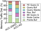
Node Cache reduces the global Points Buffer traffic and thus saves energy. Fig. 13 shows the memory traffic distributions across different data structures. In ACC-2SKD, the Points Buffer traffics would account for 53% of the total traffics without the Node Cache, and are reduced to 35% with the Node Cache. By directing 18% of the memory traffic to a smaller memory, the Node Cache reduces the energy by 5.9% (not shown). ACC-KD has very few exhaustive searches and thus much lower Points Buffer traffics. As a result, the Points Buffer traffics contribute to only 29% of the total traffic; the effect of the Node Cache is smaller.

6.5. Sensitivity Analysis

We study how the performance and energy of Tigris vary with hardware resources and software parameters.

(a) Performance vs. power.

(b) Performance comparison.

Fig. 14. Performance and power sensitivity to three hardware parameters: number of RUs, number of SUs, and number of PEs per SU. Both figures share the same legend.

Hardware Configurations

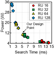
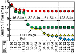
We study three key parameters: the number of RU, the number of SU, and the number of PEs per SU. We sweep all three parameters from 16, 32, 64, through 128. Fig. 14a shows the KD-tree search time and power under all 64 configurations. Overall, as performance improves the power consumption also increases. Fig. 14b shows a detailed performance comparison of different configurations, where different curves represent different RU counts and the $x$-axis sweeps the SU and PE counts.

When the RU count is low, e.g., 16 and 32, the performance is bottlenecked by the front-end. Thus, improving the back-end capabilities by increasing the SU and PE counts improves the overall speed only marginally. As the RU count increases to 64, the accelerator becomes balanced. Our design choice of 64 RUs, 32 RUs, and 32 PEs per SU sits on the “knee of the curve”, indicating a complexity-efficient design decision.

Fig. 15. Search time and energy vary with top-tree height.

Software Configurations

The results we have shown so far assume a top-tree height of 10 (about 128 children per leaf node in the top-tree). Fig. 15 shows the KD-tree search time and energy consumption as a function of the top-tree height. The performance initially increases as the top-tree height increase. This is because higher top-trees have less redundancy in exhaustive searches. However, the performance reaches a diminishing return when the top-tree height reaches around 10, beyond which the performance decreases. This is because a high top-tree requires more recursive search in the RU, thus reducing the node-level parallelism within each query that could be exploited by the SUs.

We find that the optimal top-tree height (10) is largely consistent across different KD-tree search instances in the pipeline. The optimal top-tree height mainly depends on two factors: 1) the points in a data frame, and 2) the hardware organization. Given a specific registration pipeline, different KD-tree search instances share these two factors and thus share the same optimal top-tree height.

7. Related Work

Point Cloud Registration

Point cloud registration pipelines generally fall under three categories depending on the density of points that are used for registration. On one extreme is algorithms that use all the points for registration (Besl and McKay, 1992; Behley and Stachniss, 2018; Park et al., 2017a), which tolerate outliers but are computationally prohibitive in real-time. On the other extreme are algorithms that use only (sampled) feature points (Jiang et al., 2009; Deschaud, 2018), which are efficient in compute, but could suffer from local minima.

The point cloud registration pipeline studied in this paper represents a trade-off between the two extremes, and is the predominant choice today (Xu et al., 2017; Choi et al., 2015; Huang et al., 2018; Yang et al., 2016; Zhang and Singh, 2014). It uses feature points for coarse-grained, initial estimation while using all the points for fine-tuning. While prior work proposes specific design points that make specific accuracy-speed trade-offs, we construct a flexible pipeline that let us perform design space exploration, which reveals Pareto-optimal design points that drive our performance bottleneck analysis.

Recent work has also using Deep Neural Networks (DNN) for point cloud registration. End-to-end DNNs are susceptible to and are limited to specific registration cases such as pose estimation (Wang et al., 2019). DNNs are mostly used to replace certain stages of the registration pipeline such as key point detection (Qi et al., 2017; Feng et al., 2016), normal estimation (Boulch and Marlet, 2016), description calculation (Elbaz et al., 2017), and fine-tuned ICP (Liu et al., 2006) while relying on the overall pipeline architecture as we described in Sec. 3.1.

To our best knowledge, this is also the first paper that proposes hardware accelerator for point cloud registrations while prior work mostly focuses on algorithmic developments.

KD-Tree Search Acceleration

KD-tree search is widely used in application domains beyond point cloud registration, such as graphics (Horn et al., 2007; Popov et al., 2007), data analytics (Xiao and Liu, 2010; Ooi, 1987), and image/video processing (Xu et al., 2009; Huang et al., 2010). Tigris accelerates the fundamental KD-tree search algorithm, and is applicable to these application domains as well.

Accelerating KD-tree search has been mostly explored in the context of Map-Reduce (Aly et al., 2011), GPU (Qiu et al., 2009; Gieseke et al., 2014; Heinzle et al., 2008; Kuhara et al., 2013), and FPGA (Winterstein et al., 2013). The Tigris accelerator differs from prior attempts in its systematic and comprehensive exploitation of different forms of parallelism in KD-tree search. Specifically, our Tigris accelerator exploits query-level parallelism (QLP) and node-level parallelism (NLP) both in the top-tree traversal and in the exhaustive searches. Most prior work exploits only QLP without NLP (Aly et al., 2011; Qiu et al., 2009; Heinzle et al., 2008; Kuhara et al., 2013). Buffer KD-tree (Gieseke et al., 2014) allows for NLP in the leaf nodes, but does not permit NLP in tree traversal. Heinzle et al. (Heinzle et al., 2008) exposes NLP in tree traversal, but does not exposes NLP in leaf nodes. Our accelerator design also incorporates a set of architectural mechanisms (e.g., node forwarding/bypassing, MQSN, systolic PE organization) that are unobtainable in general-purpose hardware such as GPUs.

Approximate KD-Tree Search

The approximate nature of many robotics and graphics applications that require neighbor information has spurred much interest in approximate KD-tree/KNN search algorithms (Arya et al., 1998; Miclet and Dabouz, 1983; Greenspan and Yurick, 2003; Ma and McCool, 2002; Purcell et al., 2005; Heinzle et al., 2008). Our approximate KD-tree search algorithm differs from prior work in two key ways. First, we quantify the extent to which KD-tree search can be approximated in the context of end-to-end registration accuracy while prior work mostly focuses on the accuracy of KD-tree search alone. Second, our approximate search algorithm applies to both NN search and radius search while most prior work is limited to NN search.

8. Conclusion

With the proliferation of 3D sensors and the rising need for ubiquitous 3D perception, point cloud processing is increasingly becoming the cornerstone of many machine perception applications, and architects must be ready for that. To our best knowledge, this is the first paper that comprehensively characterizes and addresses the performance bottlenecks of point cloud registration. The key to our approach is to co-design the data structure, algorithm, and the accelerator of the key compute kernel. Our work provides the first answer, not the final answer, in a promising direction of research.

References

- (1)
- sim (2018) 2018. DNN Accelerator Architecture - SIMD or Systolic? https://www.sigarch.org/dnn-accelerator-architecture-simd-or-systolic/
- xeo (2018) 2018. Intel Xeon Processor Scalable Family Datasheet, Volume Two: Registers. (2018), 55–60.
- mic (2019) 2019. Micron DDR4 Power Calculator. https://www.micron.com/~/media/documents/products/power-calculator/ddr4_power_calc.xlsm
- Aldoma et al. (2012) Aitor Aldoma, Zoltan-Csaba Marton, Federico Tombari, Walter Wohlkinger, Christian Potthast, Bernhard Zeisl, Radu Bogdan Rusu, Suat Gedikli, and Markus Vincze. 2012. Tutorial: Point cloud library: Three-dimensional object recognition and 6 dof pose estimation. IEEE Robotics & Automation Magazine 19, 3 (2012), 80–91.
- Aly et al. (2011) Mohamed Aly, Mario Munich, and Pietro Perona. 2011. Distributed kd-trees for retrieval from very large image collections. In Proceedings of the British machine vision conference (BMVC), Vol. 17.
- Arya et al. (1998) Sunil Arya, David M Mount, Nathan S Netanyahu, Ruth Silverman, and Angela Y Wu. 1998. An optimal algorithm for approximate nearest neighbor searching fixed dimensions. Journal of the ACM (JACM) 45, 6 (1998), 891–923.
- Behley and Stachniss (2018) Jens Behley and Cyrill Stachniss. 2018. Efficient surfel-based SLAM using 3D laser range data in urban environments. In Robotics: Science and Systems (RSS).
- Bentley (1975) Jon Louis Bentley. 1975. Multidimensional binary search trees used for associative searching. Commun. ACM 18, 9 (1975), 509–517.
- Besl and McKay (1992) Paul J Besl and Neil D McKay. 1992. Method for registration of 3-D shapes. In Sensor Fusion IV: Control Paradigms and Data Structures, Vol. 1611. International Society for Optics and Photonics, 586–607.
- Blais and Levine (1995) Gérard Blais and Martin D. Levine. 1995. Registering multiview range data to create 3D computer objects. IEEE Transactions on Pattern Analysis and Machine Intelligence 17, 8 (1995), 820–824.
- Boulch and Marlet (2016) Alexandre Boulch and Renaud Marlet. 2016. Deep learning for robust normal estimation in unstructured point clouds. In Computer Graphics Forum, Vol. 35. Wiley Online Library, 281–290.
- Chen and Medioni (1992) Yang Chen and Gérard Medioni. 1992. Object modelling by registration of multiple range images. Image and vision computing 10, 3 (1992), 145–155.
- Choi et al. (2015) Sungjoon Choi, Qian-Yi Zhou, and Vladlen Koltun. 2015. Robust Reconstruction of Indoor Scenes. In The IEEE Conference on Computer Vision and Pattern Recognition (CVPR).
- David et al. (2010) Howard David, Eugene Gorbatov, Ulf R Hanebutte, Rahul Khanna, and Christian Le. 2010. RAPL: memory power estimation and capping. In 2010 ACM/IEEE International Symposium on Low-Power Electronics and Design (ISLPED). IEEE, 189–194.
- Deschaud (2018) Jean-Emmanuel Deschaud. 2018. IMLS-SLAM: scan-to-model matching based on 3D data. In 2018 IEEE International Conference on Robotics and Automation (ICRA). IEEE, 2480–2485.
- Elbaz et al. (2017) Gil Elbaz, Tamar Avraham, and Anath Fischer. 2017. 3D point cloud registration for localization using a deep neural network auto-encoder. In Proceedings of the IEEE Conference on Computer Vision and Pattern Recognition. 4631–4640.
- Feng et al. (2016) Yu Feng, Alexander Schlichting, and Claus Brenner. 2016. 3D feature point extraction from LiDAR data using a neural network. International Archives of the Photogrammetry, Remote Sensing and Spatial Information Sciences-ISPRS Archives 41 (2016) 41 (2016), 563–569.
- Finkel et al. (1977) R Finkel, J Friedman, and J Bentley. 1977. An algorithm for finding best matches in logarithmic expected time. ACM Trans. Math. Software (1977), 200–226.
- Fischler and Bolles (1981) Martin A Fischler and Robert C Bolles. 1981. Random sample consensus: a paradigm for model fitting with applications to image analysis and automated cartography. Commun. ACM 24, 6 (1981), 381–395.
- Frome et al. (2004) Andrea Frome, Daniel Huber, Ravi Kolluri, Thomas Bülow, and Jitendra Malik. 2004. Recognizing objects in range data using regional point descriptors. In European conference on computer vision. Springer, 224–237.
- Geiger et al. ([n. d.]) Andreas Geiger, Philip Lenz, Christoph Stiller, and Raquel Urtasun. [n. d.]. KITTI Visual Odometry / SLAM Evaluation. http://www.cvlibs.net/datasets/kitti/eval_odometry.php. Accessed April 5, 2019.
- Geiger et al. (2012) Andreas Geiger, Philip Lenz, and Raquel Urtasun. 2012. Are we ready for autonomous driving? the kitti vision benchmark suite. In 2012 IEEE Conference on Computer Vision and Pattern Recognition. IEEE, 3354–3361.
- Gieseke et al. (2014) F. Gieseke, J. Heinermann, C. Oancea, and C. Igel. 2014. Buffer k-d trees: Processing massive nearest neighbor queries on GPUs. (2014).
- Gokturk et al. (2004) S Burak Gokturk, Hakan Yalcin, and Cyrus Bamji. 2004. A time-of-flight depth sensor-system description, issues and solutions. In 2004 Conference on Computer Vision and Pattern Recognition Workshop. IEEE, 35–35.
- Golub and Reinsch (1971) Gene H Golub and Christian Reinsch. 1971. Singular value decomposition and least squares solutions. In Linear Algebra. Springer, 134–151.
- Greenspan and Yurick (2003) Michael Greenspan and Mike Yurick. 2003. Approximate kd tree search for efficient ICP. In Fourth International Conference on 3-D Digital Imaging and Modeling, 2003. 3DIM 2003. Proceedings. IEEE, 442–448.
- Harris et al. (1988) Christopher G Harris, Mike Stephens, et al. 1988. A combined corner and edge detector.. In Alvey vision conference, Vol. 15. Citeseer, 10–5244.
- Heinzle et al. (2008) Simon Heinzle, Gaël Guennebaud, Mario Botsch, and Markus H. Gross. 2008. A Hardware Processing Unit for Point Sets. In Acm Siggraph/eurographics Symposium on Graphics Hardware.
- Horn et al. (2007) Daniel Reiter Horn, Jeremy Sugerman, Mike Houston, and Pat Hanrahan. 2007. Interactive kd tree GPU raytracing. In Proceedings of the 2007 symposium on Interactive 3D graphics and games. ACM, 167–174.
- Huang et al. (2010) Keng-Yen Huang, Yi-Min Tsai, Chih-Chung Tsai, and Liang-Gee Chen. 2010. Video stabilization for vehicular applications using SURF-like descriptor and KD-tree. In 2010 IEEE International Conference on Image Processing. IEEE, 3517–3520.
- Huang et al. (2018) Xiaoshui Huang, Jian Zhang, Qiang Wu, Lixin Fan, and Chun Yuan. 2018. A coarse-to-fine algorithm for matching and registration in 3D cross-source point clouds. IEEE Transactions on Circuits and Systems for Video Technology 28, 10 (2018), 2965–2977.
- Irani et al. (1997) Michal Irani, Benny Rousso, and Shmuel Peleg. 1997. Recovery of ego-motion using region alignment. IEEE Transactions on Pattern Analysis & Machine Intelligence 3 (1997), 268–272.
- Jiang et al. (2009) Jun Jiang, Jun Cheng, and Xinglin Chen. 2009. Registration for 3-D point cloud using angular-invariant feature. Neurocomputing 72, 16 (2009), 3839–3844.
- Johnson and Kang (1999) Andrew Edie Johnson and Sing Bing Kang. 1999. Registration and integration of textured 3D data. Image and vision computing 17, 2 (1999), 135–147.
- Klasing et al. (2009) Klaas Klasing, Daniel Althoff, Dirk Wollherr, and Martin Buss. 2009. Comparison of surface normal estimation methods for range sensing applications. In 2009 IEEE International Conference on Robotics and Automation. IEEE, 3206–3211.
- Kuhara et al. (2013) Takuya Kuhara, Takaaki Miyajima, Masato Yoshimi, and Hideharu Amano. 2013. An FPGA Acceleration for the Kd-tree Search in Photon Mapping.
- Kung (1982) Hsiang-Tsung Kung. 1982. Why systolic architectures? IEEE computer 15, 1 (1982), 37–46.
- Li et al. (2016) Shihua Li, Jingxian Wang, Zuqin Liang, and Lian Su. 2016. Tree point clouds registration using an improved ICP algorithm based on kd-tree. In 2016 IEEE International Geoscience and Remote Sensing Symposium (IGARSS). IEEE, 4545–4548.
- Liu et al. (2006) Heng Liu, Jingqi Yan, and David Zhang. 2006. Three-dimensional surface registration: A neural network strategy. Neurocomputing 70, 1-3 (2006), 597–602.
- Lowe (2004) David G Lowe. 2004. Distinctive image features from scale-invariant keypoints. International journal of computer vision 60, 2 (2004), 91–110.
- Lucas et al. (1981) Bruce D Lucas, Takeo Kanade, et al. 1981. An iterative image registration technique with an application to stereo vision. (1981).
- Ma and McCool (2002) Vincent CH Ma and Michael D McCool. 2002. Low latency photon mapping using block hashing. In Proceedings of the ACM SIGGRAPH/EUROGRAPHICS conference on Graphics hardware. Eurographics Association, 89–99.
- Miclet and Dabouz (1983) Laurent Miclet and Mhamed Dabouz. 1983. Approximative fast nearest-neighbour recognition. Pattern Recognition Letters 1, 5-6 (1983), 277–285.
- Micron Technology (2018) Inc. Micron Technology. 2018. 16Gb, 32Gb: x4, x8 3DS DDR4 SDRAM. https://www.micron.com/-/media/documents/products/data-sheet/dram/ddr4/16gb_32gb_x4_x8_3ds_ddr4_sdram.pdf
- Moré (1978) Jorge J Moré. 1978. The Levenberg-Marquardt algorithm: implementation and theory. In Numerical analysis. Springer, 105–116.
- Muja and Lowe (2014) Marius Muja and David G Lowe. 2014. Scalable nearest neighbor algorithms for high dimensional data. IEEE transactions on pattern analysis and machine intelligence 36, 11 (2014), 2227–2240.
- Ooi (1987) Beng C Ooi. 1987. Spatial kd-tree: A data structure for geographic database. In Datenbanksysteme in Büro, Technik und Wissenschaft. Springer, 247–258.
- Park et al. (2017a) Chanoh Park, Soohwan Kim, Peyman Moghadam, Clinton Fookes, and Sridha Sridharan. 2017a. Probabilistic surfel fusion for dense lidar mapping. In Proceedings of the IEEE International Conference on Computer Vision. 2418–2426.
- Park et al. (2017b) Jaesik Park, Qian-Yi Zhou, and Vladlen Koltun. 2017b. Colored point cloud registration revisited. In Proceedings of the IEEE International Conference on Computer Vision. 143–152.
- Popov et al. (2007) Stefan Popov, Johannes Günther, Hans-Peter Seidel, and Philipp Slusallek. 2007. Stackless kd-tree traversal for high performance GPU ray tracing. In Computer Graphics Forum, Vol. 26. Wiley Online Library, 415–424.
- Purcell et al. (2005) Timothy J Purcell, Craig Donner, Mike Cammarano, Henrik Wann Jensen, and Pat Hanrahan. 2005. Photon mapping on programmable graphics hardware. In ACM SIGGRAPH 2005 Courses. ACM, 258.
- Qi et al. (2017) Charles Ruizhongtai Qi, Li Yi, Hao Su, and Leonidas J Guibas. 2017. Pointnet++: Deep hierarchical feature learning on point sets in a metric space. In Advances in Neural Information Processing Systems. 5099–5108.
- Qiu et al. (2009) Deyuan Qiu, Stefan May, and Andreas Nüchter. 2009. GPU-Accelerated Nearest Neighbor Search for 3D Registration. In International Conference on Computer Vision Systems.
- Rocchini et al. (2001) CMPPC Rocchini, Paulo Cignoni, Claudio Montani, Paolo Pingi, and Roberto Scopigno. 2001. A low cost 3D scanner based on structured light. In Computer Graphics Forum, Vol. 20. Wiley Online Library, 299–308.
- Rusinkiewicz and Levoy (2001) Szymon Rusinkiewicz and Marc Levoy. 2001. Efficient variants of the ICP algorithm.. In 3dim, Vol. 1. 145–152.
- Rusu et al. (2009) Radu Bogdan Rusu, Nico Blodow, and Michael Beetz. 2009. Fast point feature histograms (FPFH) for 3D registration. In 2009 IEEE International Conference on Robotics and Automation. IEEE, 3212–3217.
- Rusu and Cousins (2011) Radu B Rusu and S Cousins. 2011. Point cloud library (pcl). In 2011 IEEE International Conference on Robotics and Automation. 1–4.
- Schwarz (2010) Brent Schwarz. 2010. LIDAR: Mapping the world in 3D. Nature Photonics 4, 7 (2010), 429.
- Scovanner et al. (2007) Paul Scovanner, Saad Ali, and Mubarak Shah. 2007. A 3-dimensional sift descriptor and its application to action recognition. In Proceedings of the 15th ACM international conference on Multimedia. ACM, 357–360.
- Shi et al. (2016) G Shi, X Gao, and X Dang. 2016. Improved ICP point cloud registration based on KDTree. 9 (01 2016), 2195–2199.
- Sipiran and Bustos (2011) Ivan Sipiran and Benjamin Bustos. 2011. Harris 3D: a robust extension of the Harris operator for interest point detection on 3D meshes. The Visual Computer 27, 11 (2011), 963.
- Steder et al. (2011) Bastian Steder, Radu Bogdan Rusu, Kurt Konolige, and Wolfram Burgard. 2011. Point feature extraction on 3D range scans taking into account object boundaries. In 2011 IEEE International Conference on Robotics and Automation. IEEE, 2601–2608.
- Stets et al. (2017) Jonathan Dyssel Stets, Yongbin Sun, Wiley Corning, and Scott W Greenwald. 2017. Visualization and labeling of point clouds in virtual reality. In SIGGRAPH Asia 2017 Posters. ACM, 31.
- Tombari et al. (2010) Federico Tombari, Samuele Salti, and Luigi Di Stefano. 2010. Unique signatures of histograms for local surface description. In European conference on computer vision. Springer, 356–369.
- Velodyne LiDAR (2018) Inc. Velodyne LiDAR. 2018. HDL-64E Data Sheet. http://velodynelidar.com/docs/datasheet/63-9194_Rev-F_HDL-64E_S3_DataSheet_Web.pdf
- Vosselman et al. (2001) George Vosselman, Sander Dijkman, et al. 2001. 3D building model reconstruction from point clouds and ground plans. International archives of photogrammetry remote sensing and spatial information sciences 34, 3/W4 (2001), 37–44.
- Wang et al. (2019) Chen Wang, Danfei Xu, Yuke Zhu, Roberto Martín-Martín, Cewu Lu, Li Fei-Fei, and Silvio Savarese. 2019. DenseFusion: 6D Object Pose Estimation by Iterative Dense Fusion. arXiv preprint arXiv:1901.04780 (2019).
- Wang et al. (2015) Xiaolong Wang, David Fouhey, and Abhinav Gupta. 2015. Designing deep networks for surface normal estimation. In Proceedings of the IEEE Conference on Computer Vision and Pattern Recognition. 539–547.
- Wang et al. (2017) Yujian Wang, Tengfei Lian, W. U. Mingming, Qian Gao, School Of Information, and Beijing Union University. 2017. Point cloud registration based on octree and KD-tree index. Engineering of Surveying & Mapping (2017).
- Whitty et al. (2010) Mark Whitty, Stephen Cossell, Kim Son Dang, Jose Guivant, and Jayantha Katupitiya. 2010. Autonomous navigation using a real-time 3d point cloud. In 2010 Australasian Conference on Robotics and Automation. 1–3.
- Winterstein et al. (2013) Felix Winterstein, Samuel Bayliss, and George A. Constantinides. 2013. FPGA-based K-means clustering using tree-based data structures. In International Conference on Field Programmable Logic & Applications.
- Xiao and Liu (2010) Chunxia Xiao and Meng Liu. 2010. Efficient mean-shift clustering using gaussian kd-tree. In Computer Graphics Forum, Vol. 29. Wiley Online Library, 2065–2073.
- Xu et al. (2017) Cheng Xu, Zhongwei Li, Zhong Kai, and Yusheng Shi. 2017. An automatic and robust point cloud registration framework based on view-invariant local feature descriptors and transformation consistency verification. Optics & Lasers in Engineering 98 (2017), 37–45.
- Xu et al. (2009) Kun Xu, Yong Li, Tao Ju, Shi-Min Hu, and Tian-Qiang Liu. 2009. Efficient affinity-based edit propagation using KD tree. In ACM Transactions on Graphics (TOG), Vol. 28. ACM, 118.
- Yang et al. (2016) Jiaqi Yang, Zhiguo Cao, and Qian Zhang. 2016. A fast and robust local descriptor for 3D point cloud registration. Information Sciences 346 (2016), 163–179.
- Zhang and Singh (2014) Ji Zhang and Sanjiv Singh. 2014. LOAM: Lidar Odometry and Mapping in Real-time.. In Robotics: Science and Systems, Vol. 2. 9.
- Zhang and Singh (2015) Ji Zhang and Sanjiv Singh. 2015. Visual-lidar odometry and mapping: Low-drift, robust, and fast. In 2015 IEEE International Conference on Robotics and Automation (ICRA). IEEE, 2174–2181.
- Zitova and Flusser (2003) Barbara Zitova and Jan Flusser. 2003. Image registration methods: a survey. Image and vision computing 21, 11 (2003), 977–1000.