Asymptotic freeness of unitary matrices in tensor product spaces for invariant states
Abstract.
In this paper, we pursue our study of asymptotic properties of families of random matrices that have a tensor structure. In [CGL17], the first- and second-named authors provided conditions under which tensor products of unitary random matrices are asymptotically free with respect to the normalized trace. Here, we extend this result by proving that asymptotic freeness of tensor products of Haar unitary matrices holds with respect to a significantly larger class of states. Our result relies on invariance under the symmetric group, and therefore on traffic probability.
As a byproduct, we explore two additional generalizations: (i) we state results of freeness in a context of general sequences of representations of the unitary group – the fundamental representation being a particular case that corresponds to the classical asymptotic freeness result for Haar unitary matrices, and (ii) we consider actions of the symmetric group and the free group simultaneously and obtain a result of asymptotic freeness in this context as well.
1. Introduction
1.1. Absorption Properties in Tensor Products
In this paper, our main aim is to study some of the mechanisms that give rise to asymptotic absorption properties of unitary random matrices. Roughly speaking, absorption phenomena refers to the observation that several interesting properties of free unitary operators remain unaffected by taking tensor products with other unitary operators.
A prototypical example of an absorption phenomenon is Fell’s absorption principle, which states that the left regular representation of a discrete group absorbs any unitary representation through tensor products (see, for instance, [Pis03, Proposition 8.1] for a precise statement). Combined with a classical computation due to Akemann and Ostrand [AO76], Fell’s absorption principle implies the following result, which has interesting applications in operator algebras (e.g., [Pis97]).
Proposition 1.1 (Norm Absorption).
Let be a Haar unitary system, i.e., free Haar unitary operators (see Definition 3). For every unitary operators , one has
In recent years, the authors of the present paper have studied several problems in free probability in which asymptotic absorption phenomena arise at the level of random unitary matrices. For example, Collins and Male proved the following finite-dimensional version of Proposition 1.1:
Proposition 1.2 ([CM14, Section 2.2.4]).
For all , let be independent Haar unitary random matrices, and let be unitary matrices of fixed dimension . Almost surely, it holds that
Proposition 1.2 follows from the strong asymptotic freeness of independent Haar unitary matrices with respect to polynomials with scalar or matrix-valued coefficients, which is the central result in [CM14].
In a slightly different direction, Collins and Gaudreau Lamarre [CGL17] proved a general result which has the following proposition as a simple special case:
Proposition 1.3.
For every , let be independent Haar unitary random matrices, and let be unitary matrices of arbitrary dimension , which may or may not depend on . In the space (where denotes the normalized trace), the family
| (1) |
converges almost surely and in expectation (Definition 5) as to a Haar unitary system.
Remark 1.
Clearly, the matrices have the same distribution (Definition 4) in the space as the matrices in the space .
The almost sure convergence of with respect to to a Haar unitary system is a classical result in free probability [HP00, Voi91]. The fact that this is preserved after taking tensor products with arbitrary unitary matrices is a special case of the tensor freeness conditions introduced in [CGL17, Definition 1.4]. We refer to Section 2.3 for more details, including an elementary proof of Proposition 1.3.
Our main purpose in this paper is to study a generalization of the absorption property stated in Proposition 1.3 (see Theorem 1.4 below for a statement of our main result). The main departure of the present paper from Proposition 1.3 is that we consider asymptotic freeness of families of the form (1) with respect to states on other than the tensor product of traces . Although this greater generality comes at a cost of making stricter assumptions on the matrices that the can absorb and replacing almost sure convergence with convergence in expectation, we show that an absorption property holds for a class of problems that go well beyond what can be explained by such simple criteria as the tensor freeness conditions of [CGL17].
1.2. Representation Theory
Representation theory has also played an important role in the study of asymptotic freeness for random matrices; see for example [Bia98, Col03]. The choice of in Equation (1) above (where denotes the entrywise complex conjugate) is a special case of the results that we treat, but it is of particular interest because it introduces additional symmetries arising from permutations of legs, and is a group morphism. That is, we are working with the representation theory of the unitary group – irreducible representations can all be obtained by taking corners of the above, that can themselves be constructed with permutations (or, more generally, elements of the commutant for the action of the group). In turn, it becomes interesting and natural to study the asymptotic properties of random unitaries that arise from representation theory, as well as families combining such unitary and permutation operators. We are able to obtain asymptotic freeness in the first case, and asymptotic freeness with amalgamation in the latter case (see Theorem 1.5 below). We note that such questions are natural from the point of view of harmonic analysis over the free group; we refer to Section 5.1 for more details.
1.3. Main Result and Corollaries
In what follows, for every , we let denote the unitary group of dimension . We use to denote a subgroup of , and we distinguish and in the cases of the orthogonal and permutation groups, respectively.
Definition 1.
Let be an integer.
-
•
A family of random matrices in is said to be -invariant if
for every .
-
•
A linear form is said to be -invariant if
for every and .
Our main result regarding absorption in tensor products is the following.
Theorem 1.4.
Let be an integer. For every , consider a family of unitary random matrices in of the form
| (2) |
where
-
•
, with , integers.
-
•
is a family of independent Haar unitary matrices ( denotes the transpose of ).
-
•
is a family of unitary random matrices in , independent of .
Remark 2.
Remark 3.
The Mingo-Speicher bound is a very powerful and fine property when analyzing the asymptotics of large random matrices by the method of moments. Its exact formulation is quite technical and requires several combinatorial definitions, which is why it is postponed until later in this article. Let us note however that the Mingo-Speicher bound holds when is a tensor product of unitary matrices of dimension ; see Remark 20.
Remark 4.
Next, we state our results concerning representation theory.
Theorem 1.5.
Let be a signature, and let be the character of the associated rational irreducible representation of , provided is large enough (see Section 5.2 for more details on this notation).
Let and let be a family of i.i.d. Haar unitary random matrices. We denote
where we recall that denotes the entrywise complex conjugate. In the space , the family converges in expectation as to a Haar unitary system.
Let be as above and be an integer. The family
is asymptotically free with amalgamation over in the tensor product representation , as .
Remark 5.
The above theorem extends the result of [MP16] to the case of arbitrary sequences of irreducible representations (associated to a given signature) in the limit of large dimension.
1.4. Organization of Paper
The remainder of this paper is organized as follows. In Section 2, we recall basic notions and results in free probability that are used in this paper. Section 3 prepares the proof of the main result, while Section 4 supplies the actual proof. Sections 5 and 6 are devoted to applications of the main result, including the proof of Theorem 1.5.
Acknowledgements
B. Collins was partially funded by JSPS KAKENHI 17K18734, 17H04823, 15KK0162 and ANR- 14-CE25-0003. P. Y. Gaudreau Lamarre was partially funded by an NSERC Postgraduate Scholarship and a Gordon Y. S. Wu Fellowship. C. Male was partially funded by a Partenariat Hubert Curien SAKURA.
Much of this work was conducted during successive visits to Kyoto University by the second- and third-named authors. The hospitality of the mathematics department at Kyoto University and the organizers of the conference “Random matrices and their applications” (held in May 2018) is gratefully acknowledged. The authors also had other occasions to work on this project during workshops held at PCMI, CRM and the Fields institute, and they grateful to these institutions for a fruitful collaborative environment during these events.
2. Background in Free Probability
In this section, we go over the basic definitions and results in free probability that are used in this paper. For a thorough introduction to the subject and its applications to random matrix theory, the reader is referred to [MS17, NS06, VDN92].
2.1. Non-commutative Probability and Haar Unitary Systems
Recall that a non-commutative probability space is defined as a pair , where is a unital algebra and is a unital () linear functional; elements of are called non-commutative random variables.
Definition 2.
A ∗-probability space is a non-commutative probability space , where is a ∗-algebra (i.e., a unital algebra endowed with an antilinear involution such that for any ) and is a state (i.e., , ). We say that is tracial whenever for any .
A non-commutative random variable in a ∗-probability space is said to be unitary if , and Haar unitary if it also satisfies for all .
Recall that unital ∗-subalgebras () of are called ∗-free if for every , , and , one has whenever and . A family of non-commutative random variables is said to be ∗-free if the collection of unital ∗-subalgebras generated by the are ∗-free.
Definition 3.
A family of non-commutative random variables is called a Haar unitary system if the are ∗-free Haar unitary non-commutative random variables.
2.2. Asymptotic Freeness of Random Matrices
Let be a probability space, and let denote the ∗-algebra of random variables with finite moments of all orders. Given , let be a random matrix with entries in . If we are given a state , then there are two natural ∗-probability spaces in which can be studied: we can consider an element of , and for every , the realization of is an element of .
Let be a collection of non-commuting indeterminates. We call a non-commutative polynomial a ∗-polynomial (here, denotes the unital algebra freely generated by the collection of non-commuting indeterminates and ). If is a monomial, then it may also be called a ∗-monomial.
Definition 4.
Given a collection of non-commutative random variables in a ∗-probability space , the ∗-distribution of is defined as the linear functional determined by the relation
Definition 5.
For every , let be a family of random matrices with entries in . Let be a family of non-commutative random variables in some ∗-probability space . We recall two notions of convergence (as ) of as elements of the space :
-
•
almost surely if for almost every realization of ,
for every ∗-polynomial P;
-
•
in expectation if for every ∗-polynomial P,
Note that here, ‘in expectation’ applies to the distribution, i.e. it tells that for any (self adjoint) polynomial, the expectation of its empirical eigenvalues distribution converges.
Remark 6.
If the limiting family in the above definition is ∗-free, then we say that is asymptotically ∗-free almost surely, in probability, or in expectation.
2.3. Tensor Freeness
Lemma 2.1 (Tensor Freeness).
Let be a Haar unitary system in , and let be a family of unitary non-commutative random variables in . Then,
is a Haar unitary system in .
Proof.
Clearly, the tensor products are unitary. Moreover, for any ∗-monomial , one has
If is trivial (i.e., for any family of unitary operators), then . Otherwise, the fact that is ∗-free implies that . Thus, is a Haar unitary system. ∎
Remark 7.
If we are given families of variables and in respective non-commutative probability spaces and , and we assume that the are ∗-free, then it is not necessarily the case that the tensor product collection
is ∗-free in . Lemma 2.1 is a special case of a more general class of examples that satisfy the tensor freeness conditions [CGL17, Definition 1.4 and Proposition 1.5], which guarantees that the freeness present in one collection propagates to the tensor product collection.
We may now prove Proposition 1.3.
Proof of Proposition 1.3.
For the sake of readability, let us denote
and
By [HP00, Voi91], converges to a Haar unitary system almost surely. Since unitary matrices are bounded in operator norm, every subsequence of has a further subsequence along which and converge almost surely to some limiting families and , respectively. Note that is the sequence of tensor products of and . Hence every limit of the subsequences is of the form (), and satisfies the hypotheses of Lemma 2.1, so it is a Haar unitary system. Since there is a single possible limit for every subsequence, converges almost surely to a Haar unitary system. Since the matrices of are bounded in operator norm, the convergence also holds in expectation. ∎
2.4. Duality of Invariance
We now explain the claim made in Remark 2 that, in the context of Theorem 1.4, we can always assume that and are both -invariant. Let be a collection of random matrices in and be a linear form.
Suppose that is -invariant, and let be a unitary matrix distributed according to the Haar measure on , independently of . Consider the collection
| (3) |
By the invariance of , for every ∗-polynomial ,
is equal in distribution to , and since is Haar distributed, the form defined as
is -invariant. Thus, if we are interested in the large limits of expectations , then there is no loss of generality in assuming that , and, in particular, that is -invariant.
Similarly, if is -invariant, then
for any , and thus there is no loss of generality in replacing by (3), which is -invariant if is independent of and Haar distributed.
2.5. Freeness with Amalgamation
The notion of freeness with amalgamation was introduced by Voiculescu as a generalization of freeness—see for example [VDN92, Section 3.8]—and appears naturally in several contexts of large random matrices. In particular, let us consider two matrices whose entries are non-commutative random variables in a space . If the entries of the respective matrices are free, then the two matrices themselves are free with amalgamation over scalar matrices [MS17, Section 9, Corollary 14]. Together with the so-called linearization trick, this result gives a powerful method to compute the spectral distribution of self-adjoint ∗-polynomials in free variables [MS17, Section 10.3]. Moreover, freeness with amalgamation over the diagonal holds for independent permutation invariant matrices with variance profiles [Shl96, ACD+21] and appear in the second order distribution of certain Wigner and deterministic matrices [Mal21].
In a ∗-algebra , we pick a unital subalgebra and we say that a unital linear functional is a conditional expectation of onto if it satisfies for all . In other words, can be seen as an orthogonal projection of onto with respect to an appropriate scalar product arising from a state preserved by . is not always guaranteed to exist; however, in the case of von Neumann algebras, there are systematic existence theorems, and existence entails uniqueness. We mostly work in the context of finite dimensional algebras which are automatically von Neumann algebras, so the existence and uniqueness is granted in the cases of interest to us. For more details we refer to Theorem 4.2 of section IX-4 of [Tak03].
Next, we get to the definition of freeness with amalgamation. In the above context of with and a conditional expectation from onto , we consider an arbitrary index set and take a family of subalgebras satisfying . The family is said to be free with amalgamation over if and only if
whenever and , with . For a systematic treatment, we refer to [MS17, Section 9.2]. One key example is as follows: if are free, then are free with amalgamation over .
Next we get to the definition of conditional distribution.
Definition 6.
Given a collection of non-commutative random variables in a ∗-probability space endowed with a conditional expectation , the ∗-conditional distribution of is defined as the linear functional determined by the relation
Finally, we can provide a definition of asymptotic freeness with amalgamation.
Definition 7.
For every , let be a family of non-commutative random variables in a ∗-probability space endowed with a conditional expectation – note here that we require to be the same for each .
Let be a family of non-commutative random variables in some ∗-probability space with a conditional expectation . Then, we say that if
| (4) |
for every , the set of all polynomials in and with coefficients from . If, in addition to (4), the -algebras are free with amalgamation over in , then we say that is asymptotically free with amalgamation over in .
3. Invariant states on tensor matrix spaces
3.1. Proof Overview Part 1
For any subgroup of , the set of -invariant linear forms on is a finite dimensional vector space. In particular, there exists a finite collection of -elementary linear forms that are -invariant and such that for every other -invariant form , one has
for some scalars .
Remark 8.
For the classical groups (such as , and ), the invariant linear forms are given by the Schur-Weyl duality. In the case of , we can compute the elementary forms and their associated constants explicitly by elementary means (see Proposition 3.1 and its proof).
The first step of the proof of Theorem 1.4 consists of identifying the -elementary linear forms. In Proposition 3.1 below, we prove that the latter are characterized by the set of partitions of (which we denote ), so that can be written as a sum of the form
A precise description of the -elementary linear forms can be found in Definition 11.
Remark 9.
A different description of these elementary functions can also be found in [Gab15].
The second step of the proof consists of bounding the decay rate of the constants that appear in the above expansion for large . In Proposition 3.2, we prove that there exist positive constants (see Definition 12) such that as .
The third and last step of our proof is to understand the growth rate of the -elementary linear forms evaluated in the matrices defined in (2), especially as compared to . This step is carried out in Section 4; see Section 4.1 for a detailed overview of this part of the argument.
The remainder of this section is devoted to the proof of the first two steps outlined above.
3.2. The -Elementary Linear Forms
3.2.1. Basis Elements
In order to describe the -elementary linear forms, we first introduce several notions in graph theory. In what follows, given an integer , we use the notation .
Definition 8.
We say that a couple is a directed graph if is a set of vertices and is a multi-set of directed edges, i.e., ordered pairs of elements of . More specifically, means that there is a directed edge from to , which we represent graphically as . We call the target of that edge, and the source. We allow to contain loops and multiple edges, and to be disconnected.
Let be an integer. A linear graph of order consists of a triplet that satisfies the following conditions.
-
•
is a finite directed graph.
-
•
maps every element of to a unique number in (thus indicating that is the -th edge for every ). We emphasize that multiple edges are associated with different numbers by , so that is a bijection from the multi-set to .
Remark 10.
We note that the set can be replaced by any totally ordered set in the above definition.
Remark 11.
We always consider linear graphs up to isomorphisms that preserve the order of the edges. That is, two linear graphs and are considered equal if there is a directed graph isomorphism such that if and only if .
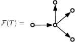
Remark 12.
A linear graph may be illustrated as follows
In the above illustration, the dots represent the vertices, the arrows represent the directed edges (making this particular example a linear graph of order ), and the value of at an edge is displayed above the edge in question.
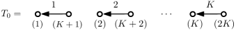
Definition 9.
We define the minimal linear graph of order , denoted , as the following linear graph. The vertices consist of the set , the edges are given by for , and we assign the order .
Remark 13.
The minimal linear graph of order is illustrated in Figure 1.
In the following definitions, we use to denote the set of partitions of a set . In the special case where for some integer , we simply denote .
Definition 10.
Let be a linear graph and be a partition of its vertex set. We denote by the quotient graph of for the partition , that is, the vertices are the blocks of , every edge of induces the edge , where are the blocks containing and respectively, and .
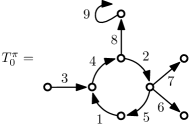
Remark 14.
A quotient of is illustrated in Figure 2.
Remark 15.
If a linear graph of order has no trivial component (i.e., single vertices with no edge), then it is a quotient of the minimal linear graph , that is, for some . In fact, since this partition is unique, the map is a bijection between and the set of linear graphs of order with no trivial component.
We may now finally define the -elementary linear forms and state the first main result of this section.
Definition 11.
Let . For every linear graph of order , we introduce an associated linear form determined by the following relation: For every ,
| (5) |
(In the above, denotes an arbitrary function from the set of vertices to , so that (5) contains summands.) We call such (unormalized) -elementary linear forms of order .
Remark 16.
In general is neither tracial nor a state. For a non-tracial counterexample, note that the linear graph of order is such that
This is clearly not tracial for . For an example that fails to be a state, note that the linear graph of order is such that
This linear form is not positive for .
Remark 17.
Clearly, the -elementary linear forms are invariant under order-preserving isomorphisms on the linear graphs. Moreover if a linear graph has a trivial component, then deleting that vertex changes the associated linear form by a multiplicative factor of . Hence it is easy to see that, up to multiplicative constants, there is a finite number of -elementary linear forms of order .
Combining this observation with Remark 15, one expects that we need only consider -elementary linear forms such that is a quotient of the minimal graph. The following proposition confirms that this is the case.
Proposition 3.1.
The set of -elementary linear forms of order generates the space of -invariant linear forms on . In particular, for every -invariant form , there exists constants (where ) such that
| (6) |
3.2.2. Control of the Coefficients
With the -elementary linear forms identified in (6), the second main result of this section concerns the control of the coefficients for large . In order to state this result, we introduce one more graph-theoretic notion.
Definition 12.
Let be a linear graph of order .
-
(1)
A cutting edge of a graph is an edge whose removal increases the number of connected components.
-
(2)
A two-edge connected graph is a connected graph with no cutting edge.
-
(3)
A two-edge connected component of a graph is a maximal connected sub-graph that is two-edge connected.
-
(4)
The forest of two-edge connected components of a graph is the graph whose vertices are the two-edge connected components of and whose edges are the cutting edges of , making links between the components that contain the source and the target of a cutting edge.
-
(5)
A trivial component of is a component consisting of a single vertex.
We denote by the number of leaves in the forest of two-edge connected components , with the convention that a trivial component has two leaves.
The following result, which is proved below in Section 3.4, contains our bound on the coefficients that appear in (6).
Proposition 3.2.
For every , as it holds that
| (7) |
Before proving Propositions 3.1 and 3.2, we take this opportunity to formulate the technical boundedness assumption on the matrices mentioned in the statement of Theorem 1.4, which is a direct consequence of the asymptotic (7):
Definition 13 (Mingo-Speicher Bound).
For each , let be a family of random matrices such that for every , there is an integer such that . We say that the sequence , , satisfies the Mingo-Speicher bound if for every , , and linear graph or order , there exists a constant independent of such that
3.3. Proof of Proposition 3.1
3.3.1. Multi-Index Kernels
For any integers , we denote by the -th elementary matrix of , that is,
where denotes the Kronecker delta function. A basis for is given by the tensor products
and an element is generically denoted as .
Let be an arbitrary linear form. We can write as a trace against a matrix, namely, for every ,
| (8) |
where . If is -invariant, then we can assume that the matrix in (8) is a -invariant deterministic matrix. Indeed, if is a random matrix uniformly distributed on , then by -invariance
where . Hence we may assume without loss of generality that .
In the sequel, we denote pairs of multi-indices as elements of , that is,
Given , we use to denote the partition of determined by the condition
In words, the blocks of are the groups of indices for which the associated integers are equal.
Example 1.
We have
Our purpose for introducing these partitions is the following trivial fact: For any two pairs of multi-indices , there exists a permutation such that if and only if (here, we denote ). Since we assume that the matrix in (8) is permutation invariant, then it follows that whenever . Consequently, if, for every , we denote by the common value of for all such that , and we define the matrix as
| (9) |
then we get the decomposition
Thus for any , one has
| (10) |
3.3.2. Injective Linear Forms and Möbius Inversion
With (10) established, it now remains to prove that each linear map is a linear combination of the -elementary linear forms. For this, we introduce the following modification of the .
Definition 14.
Let be a linear graph of order . For every , we define the injective linear form of order , denoted as
| (11) |
for every .
The relevance of injective linear forms comes from the following fact: If is such that for some , then for every , it holds that
(recall that is defined in (9)). To see this, note that, one the one hand,
On the other hand, if we enumerate the edges
of a linear graph in such a way that for every , then for any injective map , the multi-index
is such that if and only if .
We now conclude the proof of Proposition 3.1 by showing that injective linear forms can be written as linear combinations of -elementary linear forms. Recall that the set of partitions can be endowed with a natural partial order whereby if and only if every block of is contained in a block of . With this in mind, we note the following comparison between injective linear forms and -elementary linear forms:
Remark 19.
Endowed with its natural order, the poset forms a lattice [Sta12, Section 3.3]. In particular, by the Möbius inversion formula (dual form) [Sta12, Proposition 3.7.2], (12) implies that
| (13) |
where denotes the Möbius function on [Sta12, Section 3.7]. If we combine all that was shown in Section 3.3, then we see that
where
| (14) |
concluding the proof of Proposition 3.1.
3.4. Proof of Proposition 3.2
Since is a state, we know that
| (15) |
(c.f., [NS06, Proposition 3.8]). Moreover, we recall the following result of Mingo and Speicher.
Remark 20.
According to (16), any family of tensor products of unitary matrices satisfies the Mingo-Speicher bound.
Note that (15) implies that
Combining this fact with the suprema in (16) and the expansion in (6) suggests that the constants should be of order . We can make this heuristic precise with the following three results, which we prove in Sections 3.4.1–3.4.3 below.
Lemma 3.4.
For every , there exists a constant such that for every and ,
Lemma 3.5.
If , then .
Lemma 3.6.
For any , there are two constants such that for every ,
| (17) |
Indeed, if we denote , then Lemma 3.4 implies that for any matrix with unit norm. If we combine this with Lemma 3.6, then we conclude that . Given the relationship between the constants and , it follows from the Möbius inversion formula [Sta12, Proposition 3.7.1] that
where the last estimate follows from Lemma 3.5.
Remark 21.
3.4.1. Proof of Lemma 3.4
Let be fixed. Suppose that we construct random matrices such that
| (18) |
for some constant , and such that for every and , one has
| (19) |
where denotes the expected value with respect to and . Then, by (6) and (12), we see that
We now construct and . Suppose for now that we can write
where the are diagonal. Then, for every linear graph of order and matrix , it holds that
We enumerate the edges of as in such a way that for each . For every injective map , the partition of does not depend on and is denoted : two integer and are in a same block of whenever . Then we can write
| (20) |
and this quantity is independent of the choice of injective . Our objective is to define the matrices in such a way that if , then (20) is equal to . We need two ingredients to make this construction.
Firstly, for every block , we define as a diagonal matrix whose diagonal entries are i.i.d. random variables sampled according to the uniform measure on the complex roots of unity of order . In particular, for every and ,
| (21) |
Furthermore, we assume that the matrices are independent of each other.
Secondly, for every block , we define as a diagonal matrix whose diagonal entries are random variables satisfying the following conditions:
-
(1)
For every , it holds that
(22) and if two blocks are distinct, then .
-
(2)
The collections are independent of each other for different values of .
-
(3)
.
The existence of such variables is proved in Example 2 below. We also assume that the matrices are independent of .
With these definitions in mind, for every , we define the diagonal matrix , where denotes the block that contains . On the one hand, since the entries of and are uniformly bounded in , it is clear that (18) holds true. On the other hand, (20) is now equal to
| (23) |
If there exists distinct blocks and such that , then the expectation in (23) contains the product
and thus is equal to zero. Otherwise, if the fact that and are in distinct blocks of implies that (and thus since is injective), then by the independence assumptions on and we can simplify (23) to
According to (21) and (22), this expression is one if whenever and are in the same block of , and zero otherwise. In summary, (20) is equal to one if and zero otherwise, concluding the proof.
Example 2.
Let , and let be i.i.d. uniform random variables on . Next, for every , let
Then, for every binary sequence , we let
where is some function. By independence,
for every . Moreover, if are distinct, which means that for some , then the product contains the factor
whence it is zero.
3.4.2. Proof of Lemma 3.5
Given that , there exists a sequence of partitions such that for each , is obtained from by joining two blocks of into one. At the level of linear graphs, this corresponds to a sequence where each is obtained from by identifying two vertices in the latter.
On the one hand, if the two vertices that are joined together in are in the same two-edge connected component, then (i.e., the forest of two-edge connected components is unaffected by this operation). On the other hand, if we identify two distinct two-edge connected components, then the forest can be obtained from by identifying the corresponding vertices. Since this process can only decrease the number of leaves, we conclude that .
Remark 22.
By using the same argument presented here, it is easy to see that for general linear graphs and (which may contain trivial components, unlike quotients of ), if is a quotient of then .
3.4.3. Proof of Lemma 3.6
The upper bound is a direct consequence of Theorem 3.3, equation (13), and Lemma 3.5. To prove the lower bound, we present an adaptation of the example of optimality presented by Mingo and Speicher in [MS12] for their proof of Theorem 3.3 (see Example 7 and Section 5 therein).
Let . We want to find matrices of unit norm such that is of order for large . Suppose that satisfies the following:
-
•
There are cutting edges adjacent to only one leaf in .
-
•
There are cutting edges adjacent to two leaves in .
-
•
There are isolated two-edge connected components (i.e., not connected to a cutting edge). We denote the vertex sets of these connected components as .
By Definition 12, it is easily seen that .
If we denote by the -th edge of for every , then up to permuting the order of the matrices in the tensor product , or replacing some ’s by their transposes , we may assume that the following holds:
-
•
The cutting edges adjacent to one leaf are , and the cutting edges adjacent to two leaves are .
-
•
For every , the target of (i.e., ) belongs to a leaf.
Let be the partition of (defined as above Example 1) such that if and only if . We enumerate the blocks of from to , and we use to denote the number of the block containing . For any , let us define the matrix
Let be the matrix whose entries are all , let
be the Euclidean division of by , and let
where denotes the zero matrix (so long as , this can be defined without problem).
Finally, we define the matrix . It is easy to see that and all have unit norm. Moreover,
where denotes the indicator function. Thus, it suffices to prove that the number of injections such that
| (24) |
is at least of order . In order to see this, we propose to define such injections by using the following procedure.
-
(1)
For every , let .
-
(2)
Make an arbitrary choice of vertices in the isolated connected components of .
-
(3)
Make an arbitrary choice for the values
except for the requirement that the values all be distinct.
-
(4)
Let , and let be the integer such that . For every vertex in the leaf that the edge is pointing to, choose .
-
(5)
Let , and let be the integer such that . For every vertex in one of the two leaves that is connected to, choose .
-
(6)
Let , and let be the integer such that . For every , choose .
-
(7)
Finally, for every vertex for which has not yet been defined, choose .
Clearly, any injective constructed according to those conditions satisfies (24). Since is a quotient of the minimal graph , the total number of vertices is at most . Thus, for any choice made in steps (1)–(3), there is always at least one way to select the values of in such a way that steps (4)–(7) are also satisfied. Since there are
ways of selecting the values of in step (3), the result is proved.
Remark 23.
As before, the argument presented here can easily be generalized to an arbitrary linear graph possibly containing trivial components, giving the statement
for large .
4. Proof of Theorem 1.4
4.1. Proof Overview Part 2
As per Definitions 3 and 5, we aim to prove that for every nontrivial ∗-monomial , one has
as , where we recall that is the collection of matrices
Remark 24.
Recall that we call the ∗-monomial trivial if for every family of unitary operators, and nontrivial otherwise.
Remark 25.
Thanks to Propositions 3.1 and 3.2, it suffices to show that for every linear graph of order that is a quotient of , one has
| (25) |
Our method of proof for this result, which we outline in the next few paragraphs, makes significant use of ideas from traffic probability (c.f., [ACD+21, CDM16, Mal20]).
The first step for the proof of (25) consists of a linearization procedure that exhibits a linear graph and a random matrix such that
| (26) |
where is a tensor product of the matrices in and . We note that this linearization procedure already appears in [Mal20, Definition 1.7]. However, since our proof depends on several specific details of the construction of and , we provide a complete description of the linearization in Section 4.2.1 (see Definitions 15 and 16).
The second step consists of isolating the contributions of the families and to the expression on the right-hand side of (26) (see Lemma 4.1 and (33)). Our main tool for this is a splitting lemma that appears in [Mal20]. As it turns out, the contribution of can be controlled thanks to the Mingo-Speicher bound assumption (Definition 13), and the contribution of can be reduced to the asymptotic analysis of the injective trace of tensor products of i.i.d. Haar unitary random matrices (see (36)).
The third and final step in the proof of (25) consists of showing that, due to the special structure of the graph (which depends on the ∗-monomial ), the contributions of to (26) must vanish in the large limit. This part of our argument makes crucial use of a precise asymptotic for the injective trace of Haar unitary matrices from [CDM16] (see Proposition 4.2).
We now proceed to the proof of (25).
4.2. Proof of (25)
4.2.1. Linearization
Let be a linear graph of order , and let be a nontrivial ∗-monomial, which we write as
| (27) |
for some , , and .
Definition 15 (Linearized Graph).
As usual, let us enumerate ’s edges as
with the convention that . We define from by replacing each edge
by the following sequence of edges (with new vertices):
| if or , | (28) | ||||
| if . | (29) |
Thus the vertex set consists of the vertices of , with an additional new vertices for each . The edges are denoted , where and , so that , as illustrated in (28) and (29). We take the alphabetical order on the set of pairs , i.e. if and only if either , or and .
Definition 16 (Linearized Matrix).
Let us denote and . Define the matrices and as
and
We define the matrix .
We note that, by definition of (i.e., (5)), the edges in are associated with the matrices , the edges are associated with the matrices , and are associated with the . Thus, by comparing the definition of the ∗-monomial with the matrices and in the above definition, it is clear that (26) holds. We refer to the passage following [Mal20, Definition 1.7] for more details.
Remark 26.
It can be noted that and have the same forest of two-edge connected components, up to replacing every cutting edge by a sequence of consecutive cutting edges. In particular, .
4.2.2. Reduction via Injective Traces and Splitting Lemma
Given two linear graphs and , we denote if is a quotient of . According to (12),
| (30) |
From this point on until the end of the proof of (25), we fix a linear graph such that .
By Remarks 22 and 26, we see that . Consequently, by (30), in order to prove (25) it suffices to establish that
| (31) |
In order to do so, we must understand the contributions of the families and to .
Definition 17.
For , let us denote by the linear graph obtained from by:
-
•
considering only the edges numbered for and for ,
-
•
considering only the edges numbered for and for ,
and deleting all other edges. Hence is of order , whereas is of order . Note that , the vertex set of , is also the vertex set of and .
The following result, which is a direct application of [Mal20, Lemma 2.21], splits the term into two injective traces involving the matrices in and separately.
Proof.
As per Remark 25, we may assume that the matrices in are -invariant. Suppose first that we can write
for some -invariant matrices . Then, we can write and as tensor products of matrices, where the matrices in are independent of those in . In this case the result follows directly from [Mal20, Lemma 2.21] (therein, is used to denote , and the vertex sets and can be taken to be both equal to , since we allow connected components consisting of a single vertex in and ). Since and the expression of [Mal20, Equation (2.14)] are linear, we conclude that the result holds for general by representing the latter as a sum of tensor products of -invariant matrices. ∎
The proof of (25) is therefore reduced to showing that
| (33) |
as , where
| (34) |
Note that the quotient relation between linear graphs induces a partial order that makes the set of linear graphs of a fixed order a lattice. Thus, although may contain trivial components, the same argument used in (12) yields
| (35) |
This then implies by Möbius inversion [Sta12, Proposition 3.7.2] that
Since implies that (Remark 22), the assumption that satisfies the Mingo-Speicher bound (Definition 13) implies that the term is bounded. Thus, (33) follows if we show that , and that
| (36) |
This is the subject of Sections 4.2.3 and 4.2.4, respectively.
4.2.3. Analysis of
We begin with some definitions.
Definition 18.
Let be the set of connected components of the graphs and , called colored components. Let be the undirected graph, called the graph of colored components, defined as follows:
-
(1)
The vertices of are the connected components in .
-
(2)
Let be connected components of and , respectively. For every vertex of that is in both and , we associate an undirected edge in connecting and .
Definition 19.
Let be a graph. For every , we let denote the number of edges in that are adjacent to .
Given that there is a one-to-one correspondence between the vertices of and the edges of , it is easy to see that
Hence, since is additive with respect to connected components, we can reformulate as
In order to analyze this quantity, we propose a modification of the graph .
Let be a connected component with no cutting edge, and which is a leaf in the graph . Since has no cutting edge, then . Since is a leaf in , the single edge in adjacent to it adds a contribution of to the quantity . In particular, if we remove and its adjacent edge from , then the quantity
remains unchanged.
Let , and for every , let be the graph obtained from by removing all connected components with no cutting edges that are leaves in , as well as their adjacent edges. Clearly, there exists some such that , namely, the first such that has no leaf which is a connected component with no cutting edge. We refer to in the sequel as the pruning of . By arguing as in the previous paragraph, we see that
| (37) |
For every , let denote the number of leaves in that do not contain a vertex that is attached to another connected component , and let be the remaining leaves. We claim that for every ,
| (38) |
Indeed, the first inequality holds since there are no connected components without cutting edges in (and thus is actually equal to the number of leaves in ), and the second inequality is valid because every leaf counted by must already appear in . By combining (37) with (38), we finally conclude that , as desired.
4.2.4. Limiting Injective Forms of Haar Unitary Matrices
To conclude the proof of (25), it now only remains to establish (36). For this, we must understand the asymptotic behaviour of the term for large . In order to state the result we need, we recall a few more notions from graph theory.
Definition 20.
Let be a linear graph. For every edge in , we denote .
-
(1)
A path of (also called a walk) is a sequence of edges of , , and an order of passage for each step such that the target of is the source of .
-
(2)
A cycle of (also called closed walk) is a path such that the target of is the source of (with the same notation as above).
-
(3)
A circuit of is a cycle where no edge is visited twice.
-
(4)
A simple cycle of is a cycle where no vertex is visited twice, except for the first (and last) vertex.
-
(5)
We say that is a forest of cacti whenever each edge belongs to exactly one simple cycle.
-
(6)
A forest of cacti is said to be well oriented when the edges of a same cycle follow the same orientation.
Remark 27.
It is worth noting here that the notion of cactus presented in the above definition differs from an arguably more common definition, which is to assume that every edge belongs to at most one simple cycle.

Definition 21.
Let be a well oriented forest of cacti of order , and let and be two labellings of ’s edges.
-
(1)
If for every simple cycle , then we say that is well colored.
-
(2)
If every simple cycle of is of even size and the values of alternate along indices of each cycle (i.e., we can enumerate the edges of every simple cycle in such a way that if is even and if is odd), then we say that is alternated.
If is both well colored and alternated, we say that it is valid.
The following proposition, which is a special case of a more general result in [CDM16], is based on the Weingarten calculus [Col03, CS06]. It can also be derived from the limiting traffic distribution of a single Haar unitary matrix and the rule of traffic independence [Mal20].
Proposition 4.2 ([Mal20, Proposition 3.7]).
Let be a linear graph of order , and let and be labellings of ’s edges. If we denote by the number of connected components of , then the limit
| (39) |
exists and is finite. More precisely, we have that
where the above product is taken over all simple cycles of , and denotes the length of a particular cycle .
We recall that the edges of are enumerated by pairs of the form
endowed with the alphabetical order. Moreover, we recall that the ∗-monomial is written as
for some and (see (27)). We note that and naturally induce a labelling of ’s edges (which we also denote as and for simplicity) as follows: For every and , we let
Thus, it follows from Proposition 4.2 that
| (40) |
We remark that the renormalization of in (40) is different from , which is what we use in (36). However, it is clear from Definition 12 that , and that there are cases where (for instance when has no cutting edge). Therefore, the asymptotic (36) is proved if we show that is not a valid well oriented forest of cacti. In order to prove this, we compare some basic properties of valid well oriented forests of cacti with the structure that the nontrivial ∗-monomial imposes on .
The first property of well oriented forests of cacti that is of interest to us is a type of nested simple cycle structure. This can be described effectively using noncrossing partitions.
Definition 22.
A partition () is said to be noncrossing if no two blocks cross each other, that is, there exist no two blocks in and , such that . A block in a noncrossing partition is said to be inner if there exist another block such that , which also implies that .
Lemma 4.3.
Every connected component of a well oriented forest of cacti has a circuit that follows the orientation of ’s edges. In particular, if is such a circuit, then the partition defined by
is a noncrossing partition with blocks of even size.
Proof.
The existence of the circuit follows from the fact that each vertex in a forest of cacti must be contained in a unique simple cycle. Next, suppose by contradiction that there exists such that and . Then, is part of a simple cycle that is entirely contained in the sequence , and which does not contain . However, since , this means that must be part of two distinct simple cycles (one of which contains ), which is a contradiction. ∎
Let be the disjoint union of the graphs represented by the paths defined in (28)-(29) for and the vertices coming from the paths for (i.e., we include all vertices that appear in the paths for , but we exclude the edges). With notations as in (28) and (29), for we call and respectively the source and the target of , whereas for we interchange the role of the vertices, calling the target and the source of . We recall (Definitions 15 and 17) that is a quotient of .
With this in mind, we have the following consequence of Lemma 4.3.
Lemma 4.4.
If is valid, then it is an edge-disjoint union of circuits that are compositions of the paths (here, we say that two paths and can be composed if the target of the last step of is the source of the first step of ).
Proof.
If is a forest of cacti, then there is no vertex of odd degree. In particular, every vertex of degree one in (which is either a target or source of a path ) is identified with at least one other such vertex in the quotient . We may then first form a quotient of by composing the paths whose targets and sources have been identified as in , and then obtain by adding more identifications. ∎
Next, in order to better understand the structure that imposes on , we introduce the concept of a word induced by a path.
Definition 23.
Let be a graph of order with two labellings and . Let be a path of which follows the edge orientations in . We denote by the ∗-monomial
Lemma 4.3 has the following consequence.
Lemma 4.5.
Let be valid. If is a circuit as in Lemma 4.4 of which agrees with the edge orientations in , then is trivial.
Proof.
Suppose first that is a simple cycle. Since is valid, it is well colored and alternated, and thus we can write
for some integer and index . Clearly, this -word reduces to 1 when evaluated in unitary operators.
More generally, let us denote , and let the noncrossing partition be defined as in Lemma 4.3. Suppose that denotes the (smaller) circuit obtained from by removing the edges contained in any inner block of . By repeating the argument used in the case where was a simple cycle, it is easy to see that for any family of unitary operators , since every inner block of corresponds to an uninterrupted simple cycle within . By removing each inner block from one by one, we are eventually left with a simple cycle, concluding the proof. ∎
We now have all the necessary ingredients to conclude the proof of (25). Recalling from (27) that , we define the mirrored word . Suppose by contradiction that is valid. For each , it holds that for and for .
By Lemma 4.4, is quotient of a well oriented forest of cacti such that if is a circuit of a connected component of which agrees with the edge orientations in , then it must be the case that is a non commutative product of powers of and , such as for .
Therefore, Lemma 4.5 implies that is trivial. Let be a Haar unitary system. Since (as is a nontrivial ∗-monomial), and by Nielsen-Schreier theorem, the group generated by and is either or . The group cannot be , because if that were the case, then would not be trivial. Thus, the group generated by and must be . Consequently, without loss of generality, we can assume there exists a , such that . But the mirror operation is an involution, so and then . Since is non trivial this is absurd.
We therefore finally conclude that cannot be valid, whence (33) holds, as desired.
5. Proof of Theorem 1.5
5.1. Asymptotic representation theory
This manuscript deals with asymptotic freeness for tensors. In the case of unitary operators, it is possible to turn this question into a problem of harmonic analysis over the free group. This is what we would like to discuss in this section.
Voiculescu established asymptotic freeness for sequences of group in the large dimension limit in [Voi91, Voi98]. However, long before his asymptotic freeness results in the nineties, he had already studied the limit of unitary groups, from the slighly different point of view of representation theory [SV75]. His result here generalized results of Thoma [Tho64], and it was discovered in [VK82] that finite dimension group approximation was a natural way to prove the results.
A way to reformulate some questions of this paper is: consider sequences of unital functions of positive type (sometimes called positive definite) on the unitary group . Under which conditions will be asymptotically free almost surely for i.i.d. Haar unitary variables in ?
We restrict our question slightly further – without however missing any example provided by the results contained in this manuscript – by requiring in addition the limit to be Haar distributions, i.e. all non-trivial moments tend to zero. An important observation is that if satisfy this condition, then the same will hold true for any polynomial in these, as soon as it does not have any constant component. If one wants to ensure that this polynomial operation remains a state, it is enough to require that the coefficients of each product be non negative, and that they add up to . Indeed, in terms of representation theory, taking a product corresponds to a tensor product, and taking a barycenter (with rational coefficients) corresponds to taking direct sums of representations. Put differently, this paper can be interpreted as saying that many states that are not tracial yield also asymptotic freeness.
5.2. Asymptotic freeness for any representation
We begin by proving the asymptotic freeness of with respect to arbitrary irreducible rational representations. We first recall a result of Mingo and Popa.
Theorem 5.1 ([MP16]).
The family
converges to a Haar unitary system almost surely and in expectation as in the space .
Remark 28.
[MP16] states in more generality the result for unitarily invariant random matrices in the sense of expectation, together with the second order asymptotic freeness (see Corollary 20 and Proposition 38 therein). This implies that the variance of the -distribution is of order , and thus almost sure convergence.
It is known that irreducible representations of are in a one to one correspondance with the signatures associated with their characters, i.e., sequences of integers. If , then the associated representation is polynomial, otherwise it is rational.
For the purpose of asymptotics, it is convenient to characterize the irreducible representation by a pair of Young tableaux (known as the signatures, e.g., [Ž73]). That is, given a sequence of integers, if we let be the largest index such that , then the data
with and
characterizes the rational irreducible representation. Calling (resp. ) the length, i.e., the number of non-zero elements of the sequence of integers (resp. ), we have that . In other words, in order to pass from the highest weights in the Cartan-Weyl theory to the representation with signatures , one has to pad “zero” highest weights in the middle of the sequence in a unique way to ensure completion into a non-increasing sequence of integers, as follows:
Conversely, a pair of tableaux characterizes a rational irreducible representation of the -dimensional unitary group as soon as ; indeed, for fixed choices of , we are interested in the behaviour of the sequence of irreducible representations of associated to when .
5.3. Asymptotic freeness with amalgamation
We now conclude this section by proving the statement in Theorem 1.5 regarding asymptotic freeness of with amalgamation over . Let . Given unitary matrices , we consider the representation of the group , where each generator of the free group is sent to , and acts by permutation of legs of the tensor (we use to denote the function that maps each permutation to the associated matrix that permutes the legs of the tensor).
Theorem 5.2.
The map extends to a random representation of the free group on generators in . Likewise, the map yields a representation of in and these two representations commute, therefore we have a random representation of the group . This random representation converges pointwise to the character associated to the left regular representation of as (i.e. for the neutral element, and zero for all others).
Proof.
It is enough to prove that for a non trivial word , . If the component is not the identity, the character is bounded above by a product of normalized traces of unitaries times therefore it goes to zero. If component is the identity, then the value of the character is , where is obtained from the random representation of . In this case, asymptotic freeness is known, and this quantity converges either to zero or one, depending on whether the word is trivial or not. The power of this quantity converges to the same limit and this concludes the proof. ∎
Remark 29.
From Theorem 5.2, we then obtain the desired result as corollary:
Proof of Theorem 1.5 Part 2.
The asymptotic freeness of with amalgamation over follows directly from Theorem 5.2, modulo the following two facts:
- (1)
-
(2)
The free product of , -times, amalgamated over under the canonical identification, is isomorphic to .
(As a remark, we point out that this result yields another proof of the asymptotic freeness with respect to arbitrary characters, which we have proved in Section 5.2.) ∎
6. Discussion
6.1. Strong Asymptotic Freeness
Given that absorption properties regarding asymptotic ∗-freeness of tensor products hold with rather general assumptions, it is natural to wonder if a similar phenomenon occurs with strong asymptotic freeness. Unfortunately, the following counterexample shows that strong asymptotic ∗-freeness is not as easily preserved by tensor products.
Example 3.
Let be independent by Haar unitary random matrices, where . We claim that are not strongly asymptotically -free. To see this, let be the limits in -distribution of the , and let be the limits of the . If strong asymptotic -freeness holds, then
According to Fell’s absorption principle (in particular, Proposition 1.1), the fact that the are -free Haar unitary variables implies that
For each , let denote the canonical basis of , and let us define It is easy to see that for any unitary matrix , . Therefore,
which is a contradiction as soon as . For the case we cannot derive a contradiction immediately, however we can get one along the same lines by exhibiting three or more free elements in the free group generated by two elements, and reason along the same lines as the argument above.
6.2. Renormalizations
In the framework of traffic spaces [Mal20], one considers families of random matrices such that
| (41) |
is of order 1 for large , where is the number of connected components of ; see for instance Proposition 4.2. This is very different from the renormalization which naturally arises in this article, namely by defining
| (42) |
where we recall that is the number of leaves of the tree of two-edge connected components of (Definition 12). It is interesting to note that our main result leads to an analogue of the asymptotic traffic independence in this regime:
Proposition 6.1.
Remark 30.
The limit depends only on and , and it differs from the so-called traffic free product of the individual distributions.
Proof of Proposition 6.1.
We denote by the function defined as with instead of . Then is bounded if and only if is bounded since they are related by Möbius formulas and by Lemma 3.5. Let and , for some indices ’s and ’s. From (30), changing only the definitions of and the computation remains valid, and we get: for any linear graph ,
where and are the subgraphs of consisting of edges associated with and respectively, and we recall that is defined as in (34). ∎
References
- [ACD+21] Benson Au, Guillaume Cébron, Antoine Dahlqvist, Franck Gabriel, and Camille Male. Freeness over the diagonal for large random matrices. Ann. Probab., 49(1):157–179, 2021.
- [AGZ10] Greg W. Anderson, Alice Guionnet, and Ofer Zeitouni. An introduction to random matrices, volume 118 of Cambridge Studies in Advanced Mathematics. Cambridge University Press, Cambridge, 2010.
- [AO76] Charles A. Akemann and Phillip A. Ostrand. Computing norms in group -algebras. Amer. J. Math., 98(4):1015–1047, 1976.
- [Bia98] Philippe Biane. Representations of symmetric groups and free probability. Adv. Math., 138(1):126–181, 1998.
- [CDM16] Guillaume Cébron, Antoine Dahlqvist, and Camille Male. Universal constructions for spaces of traffics. arXiv:1601.00168v1, 2016.
- [CGL17] Benoit Collins and Pierre Yves Gaudreau Lamarre. -freeness in finite tensor products. Adv. in Appl. Math., 83:47–80, 2017.
- [CM14] Benoît Collins and Camille Male. The strong asymptotic freeness of Haar and deterministic matrices. Ann. Sci. Éc. Norm. Supér. (4), 47(1):147–163, 2014.
- [Col03] Benoît Collins. Moments and cumulants of polynomial random variables on unitary groups, the Itzykson-Zuber integral, and free probability. Int. Math. Res. Not., (17):953–982, 2003.
- [CS06] Benoît Collins and Piotr Śniady. Integration with respect to the Haar measure on unitary, orthogonal and symplectic group. Comm. Math. Phys., 264(3):773–795, 2006.
- [EI16] Takumi Enomoto and Masaki Izumi. Indecomposable characters of infinite dimensional groups associated with operator algebras. J. Math. Soc. Japan, 68(3):1231–1270, 2016.
- [Gab15] F. Gabriel. Combinatorial theory of permutation-invariant random matrices i: Partitions, geometry and renormalization. arXiv:1503.02792, 2015.
- [HP00] Fumio Hiai and Dénes Petz. Asymptotic freeness almost everywhere for random matrices. Acta Sci. Math. (Szeged), 66(3-4):809–834, 2000.
- [Mal20] Camille Male. Traffic distributions and independence: permutation invariant random matrices and the three notions of independence. Mem. Amer. Math. Soc., 267(1300), 2020.
- [Mal21] Camille Male. Freeness over the diagonal and global fluctuations of complex wigner matrices. J. Oper. Theory, 85(1), 2021.
- [MP16] James A. Mingo and Mihai Popa. Freeness and the transposes of unitarily invariant random matrices. J. Funct. Anal., 271(4):883–921, 2016.
- [MS12] James A. Mingo and Roland Speicher. Sharp bounds for sums associated to graphs of matrices. J. Funct. Anal., 262(5):2272–2288, 2012.
- [MS17] James A. Mingo and Roland Speicher. Free probability and random matrices, volume 35 of Fields Institute Monographs. Springer, New York; Fields Institute for Research in Mathematical Sciences, Toronto, ON, 2017.
- [NS06] Alexandru Nica and Roland Speicher. Lectures on the combinatorics of free probability, volume 335 of London Mathematical Society Lecture Note Series. Cambridge University Press, Cambridge, 2006.
- [Pis97] Gilles Pisier. Quadratic forms in unitary operators. Linear Algebra Appl., 267:125–137, 1997.
- [Pis03] Gilles Pisier. Introduction to operator space theory, volume 294 of London Mathematical Society Lecture Note Series. Cambridge University Press, Cambridge, 2003.
- [Shl96] Dimitri Shlyakhtenko. Random Gaussian band matrices and freeness with amalgamation. Internat. Math. Res. Notices, (20):1013–1025, 1996.
- [Sta12] Richard P. Stanley. Enumerative combinatorics. Volume 1, volume 49 of Cambridge Studies in Advanced Mathematics. Cambridge University Press, Cambridge, second edition, 2012.
- [SV75] Şerban Strătilă and Dan Voiculescu. Representations of AF-algebras and of the group . Lecture Notes in Mathematics, Vol. 486. Springer-Verlag, Berlin-New York, 1975.
- [Tak03] M. Takesaki. Theory of operator algebras. II, volume 125 of Encyclopaedia of Mathematical Sciences. Springer-Verlag, Berlin, 2003. Operator Algebras and Non-commutative Geometry, 6.
- [Tho64] Elmar Thoma. Die unzerlegbaren, positiv-definiten Klassenfunktionen der abzählbar unendlichen, symmetrischen Gruppe. Math. Z., 85:40–61, 1964.
- [VDN92] D. V. Voiculescu, K. J. Dykema, and A. Nica. Free random variables, volume 1 of CRM Monograph Series. American Mathematical Society, Providence, RI, 1992. A noncommutative probability approach to free products with applications to random matrices, operator algebras and harmonic analysis on free groups.
- [VK82] A. M. Vershik and S. V. Kerov. Characters and factor-representations of the infinite unitary group. Dokl. Akad. Nauk SSSR, 267(2):272–276, 1982.
- [Voi91] Dan Voiculescu. Limit laws for random matrices and free products. Invent. Math., 104(1):201–220, 1991.
- [Voi98] Dan Voiculescu. A strengthened asymptotic freeness result for random matrices with applications to free entropy. Internat. Math. Res. Notices, (1):41–63, 1998.
- [Ž73] D. P. Želobenko. Compact Lie groups and their representations. American Mathematical Society, Providence, R.I., 1973. Translated from the Russian by Israel Program for Scientific Translations, Translations of Mathematical Monographs, Vol. 40.