Convex Formulation of Overparameterized Deep Neural Networks

Abstract

Analysis of over-parameterized neural networks has drawn significant attention in recent years. It was shown that such systems behave like convex systems under various restricted settings, such as for two-level neural networks, and when learning is only restricted locally in the so-called neural tangent kernel space around specialized initializations. However, there are no theoretical techniques that can analyze fully trained deep neural networks encountered in practice. This paper solves this fundamental problem by investigating such overparameterized deep neural networks when fully trained. We generalize a new technique called neural feature repopulation, originally introduced in (Fang et al., 2019a, ) for two-level neural networks, to analyze deep neural networks. It is shown that under suitable representations, overparameterized deep neural networks are inherently convex, and when optimized, the system can learn effective features suitable for the underlying learning task under mild conditions. This new analysis is consistent with empirical observations that deep neural networks are capable of learning efficient feature representations. Therefore, the highly unexpected result of this paper can satisfactorily explain the practical success of deep neural networks. Empirical studies confirm that predictions of our theory are consistent with results observed in practice.

1 Introduction

Deep Neural Networks (DNNs) have achieved great successes in numerous real applications, such as image classification (Krizhevsky et al.,, 2012; Simonyan & Zisserman,, 2014; He et al.,, 2016), face recognition (Sun et al.,, 2014), video understanding (Yue-Hei Ng et al.,, 2015), neural language processing (Bahdanau et al.,, 2014; Luong et al.,, 2015), etc. However, compared to the empirical successes, the theoretical understanding of DNNs falls far behind. Part of the reasons might be the general perception that DNNs are highly non-convex learning models.

In recent years, there has been significant breakthroughs (Mei et al.,, 2018; Chizat & Bach,, 2018; Du et al., 2019a, ; Allen-Zhu et al.,, 2019) in analyzing over-parameterized Neural Networks (NNs), which are NNs with massive neurons in hidden layer(s). It is observed from empirical studies that such NNs are easy to train (Zhang et al.,, 2016). And it was noted that under some restrictive settings, such as two-level NNs (Mei et al.,, 2018; Chizat & Bach,, 2018) and when learning is only restricted locally in the neural tangent kernel space around certain initializations (Du et al., 2019a, ; Allen-Zhu et al.,, 2019), NNs behave like convex systems when the number of the hidden neurons goes to infinity. Unfortunately, to the best of our knowledge, existing studies failed to analyze fully trained DNNs encountered in practice. In particular, the existing analysis cannot explain how DNNs can learn discriminative features specifically for the underlying learning task, as observed in real applications (Zeiler & Fergus,, 2014).

To remedy the gap between the existing theories and practical observations, this paper develops a new theory that can be applied to fully trained DNNs. Following a similar argument in the analysis of two-level NNs in Fang et al., 2019a , we introduce a new theoretical framework called neural feature repopulation (NFR), to reformulate over-parameterized DNNs. Our results show that under suitable conditions, in the limit of infinite number of hidden neurons, DNNs are infinity-dimensional convex learning models with appropriate re-parameterization. In our framework, given a DNN, the hidden layers are regraded as features and the model output is given by a simple linear model using features of the top hidden layer. The output of a DNN, in the limit of infinite number of hidden neurons, depends on the distributions of the features and the final linear model. We show that using the NFR technique, it is possible to decouple the distributions of the features from the loss function and their impact can be integrated into the regularizer. This largely simplifies the objective function. Under our framework, the feature learning process is characterized by the regularizer. When suitable regularizers are imposed, the overall objective function under special re-parameterization is convex, and it guarantees that the DNN learns useful feature representations under mild conditions. Unlike the Neural Tangent Kernel approach, our theoretical framework for DNN does not require the variables to be confined in an infinitesimal region. Therefore it can explain the ability of fully trained DNNs to learn target feature representations. This matches the empirical observations.

More concretely, the paper is organized as follows. Section 2 discusses the relationship of this paper to earlier studies, especially recent works on the analysis of over-parameterized NNs. Section 3 introduces the definition of discrete DNNs, and we introduce an importance weighting formulation which eventually motivates our NFR formulation. Section 4 describes the continuous DNN when the number of hidden nodes goes to infinity in the discrete DNN. In this formulation, each hidden layer is represented by a distribution over its hidden nodes that represent functions of the input. We can further interpret a discrete DNN as a random sample of hidden nodes from a continuous DNN at each layer, and then study the variance of such random discretization. The variance formula motivates the study of a class of regularization conditions for DNNs. Using the connection between discrete and continuous (over-parameterized) DNNs, we introduce the process of NFR in Section 5. In this process, an over-parameterized DNN can be reformulated as a convex system that learns effective feature representations for the underlying task. Experiments are presented in Section 6 to demonstrate that our theory is consistent with empirical observations. In Section 6.1, we consider a new optimization procedure inspired by the NFR view to verify its effectiveness. Final remarks are given in Section 7.

The main contributions of this work can be described as follows.

• We propose a new framework for analyzing overparameterized deep NN called neural feature repopulation (NFR). It can be used to remove the effect of learned feature distributions over hidden nodes from the loss function, and confine the effect only to the regularizer. This significantly simplifies the objective function.

• We study a class of regularizers. With these regularizers, the over-parameterized DNN can be reformulated as a convex system using NFR under certain conditions. The global solution of such a convex model guarantees useful feature representations for the underlying learning task.

• Our theory matches empirical findings, and hence this theory can satisfactorily explain the success of fully trained overparameterized deep NNs.

We shall also mention that the paper focuses on presenting the intuitions and consequences of the new framework. In order to make the underlying ideas easier to understand, some of the analyses are not stated with complete mathematical rigor. A more formal treatment of the results will be left to future works.

Notations. For a vector $x\in{\mathbb{R}}^{d}$, we denote $\|\cdot\|_{\_}1$ and $\|\cdot\|$ to be its $\ell_{\_}1$ and $\ell_{\_}2$ norms, respectively. We let $x^{\top}$ be the transpose of $x$ and let $x_{\_}k$ be the value of $k$-th dimension of $x$ with $k=1,\ldots,d$. Let $[m]=\{1,2,...,m\}$ for a positive integer $m$. For a function $f(x):\mathbb{R}^{d}\rightarrow\mathbb{R}$, we denote $\nabla_{\_}{x}f$ to be the gradient of $f$ with respect to $x$. For two real valued numbers $a$ and $b$, we denote $a\vee b$ to be $\max(a,b)$. If $\mu$ and $\nu$ are two measures on the same measurable space, we denote $\mu\ll\nu$ if $\mu$ is absolutely continuous with respect to $\nu$, and $\mu\sim\nu$ if $\mu\ll\nu$ and $\nu\ll\mu$.

2 Related Work

In recent years, there have been a number of significant developments to obtain better theoretical understandings of NNs. We review works that are most related to this paper. The main challenge for developing such theoretical analysis is the non-convexity of the NN model, which implies that first-order algorithms such as (Stochastic) Gradient Descent may converge to local stationary points.

In some earlier works, a number of researchers (Hardt & Ma,, 2016; Freeman & Bruna,, 2016; Brutzkus & Globerson,, 2017; Boob & Lan,, 2017; Ge et al.,, 2017; Bakshi et al.,, 2018; Ge et al.,, 2018) studied NNs under special conditions either for input data or for NN architectures. By carefully characterizing the geometric landscapes of the objective function, these early works showed that some special NNs satisfy the so-called strict saddle property (Ge et al.,, 2015). One can then use some recent results in nonconvex optimization (Jin et al.,, 2017; Fang et al.,, 2018; Fang et al., 2019b, ) to show that first-order algorithms for such NNs can efficiently escape saddle points and converge to some local mimima.

Table 1: Some Representative Works on the Three Views for Over-parameterize NNs

Views	Two-level	Multi-level
Mean Field	Mei et al., 2018 Chizat & Bach, 2018	Nguyen, 2019
Neural Tangent Kernel	Du et al., 2019b Li & Liang, 2018	Du et al., 2019a Allen-Zhu et al., 2018, 2019
Neural Feature Repopulation	Fang et al., 2019a	this work

A number of more recent theoretical analysis focused on over-parameterized NNs, which are NNs that contain a large number of hidden nodes. The motivation of overparameterization comes from the empirical observation that over-parameterized DNNs are much easier to train and often achieve better performances (Zhang et al.,, 2016). When the number of hidden units goes to infinity, the network naturally becomes a continuous NN. In the continuous limit, the resulting networks are found to behave like convex systems under appropriate conditions. Our work follows this line of the research. In the following, we review the three existing points of views, i.e., the mean field view, the neural tangent kernel view, and the NFR view. Due to the space limitation, Table 1 only summarizes some of the representative studies on these views, and additional studies are discussed in the text below.

2.1 Mean Field View for Over-parameterized Two-level NNs

The Mean Field approach has been recently introduced to analyze two-level NNs. This point of view models the continuous NN as a distribution over the NN’s parameters, and it studies the evolution of the distribution as a Wasserstein gradient flow during the training process (Mei et al.,, 2018; Chizat & Bach,, 2018; Sirignano & Spiliopoulos,, 2019; Rotskoff & Vanden-Eijnden,, 2018; Mei et al.,, 2019; Dou & Liang,, 2019; Wei et al.,, 2018). The process can be represented by a partial differential equation, which can be further studied mathematically. For two-level continuous NNs, it is known that the objective function with respect to the distribution of parameters is convex in the continuous limit. And it can be shown that (noisy) Gradient Decent can find global optimal solutions under certain conditions.

The benefit of the Mean Field View is that it mathematically characterizes the entire training process of NN. However, it relies on the special observation that a two-level continuous NN is naturally a linear model with respect to the distribution of NN parameters, and this observation is not applicable to multi-level architectures. Consequently, it is difficult to generalize the Mean Field view to analyze DNNs without losing convexity. In fact, in a recent attempt Nguyen, (2019), the technique of Mean Field view is applied to DNNs, but the author could only obtain the evolution dynamic equation for Gradient Descent. Since DNN is no longer a linear model with respect to the distribution of the parameters, Nguyen, (2019) failed to show that the system is convex. Therefore similar to the situation of Stochastic Gradient Descent for discrete DNNs, Gradient Descent for continuous DNNs can still lead to suboptimal solutions.

2.2 Neural Tangent Kernel View for Over-parameterized DNNs

One remarkable direction to extend the Mean Field view to analyze DNNs is to restrict the DNN parameters in an infinitesimal region around the initial values. With proper scaling and random initialization, DNN can be regarded as a linear model in this infinitesimal region, which makes the training dynamics solvable. This point of view is referred to as the Neural Tangent Kernel (NTK) view, since the evolution of the trainable parameters, when restricted to the infinitesimal region, can be characterized by a kernel in the tangent space. There have been a series of studies based on this point of view, which give various theoretical guarantees including sharper convergence rates and tighter generalization bounds with early stopping for both two-layer NNs (Du et al., 2019b, ; Li & Liang,, 2018; Arora et al., 2019b, ; Su & Yang,, 2019) and DNNs with more complex structures (Du et al., 2019a, ; Lee et al.,, 2018; Jacot et al.,, 2018; Allen-Zhu et al.,, 2018, 2019; Zou et al.,, 2018).

However, as point out by Fang et al., 2019a , NTK is not a satisfactory mathematical model for NNs. This is because NTK essentially approximates a nonlinear NN by a linear model of the infinite dimensional random features associated with the NTK, and these features are not learned from the underlying task. In contrast, it is well known empirically that the success of NNs largely relies on their ability to learn discriminative feature representations (LeCun et al.,, 2015). Therefore the NTK view does not match the empirical observations.

A recent attempt to justify NTK is given by Arora et al., 2019a , who proposed an efficient exact algorithm to compute Convolutional Neural Tangent Kernel. However, the classification accuracy of $77\%$ on the CIFAR-10 dataset obtained by kernel regression using NTK is $5\%$ less than that of the corresponding fully trained Convolutional NNs , and is at least $15\%$ less than the accuracies achieved by modern NNs such as ResNet (He et al.,, 2016).

2.3 Neural Feature Repopulation for Over-parameterized NNs

More recently, Fang et al., 2019a proposed the NFR view for analyzing two-level NNs. While the Mean Filed view does not have the concept of “layer” in its analysis of two-level NNs, the NFR view treats the top-layer linear model and the bottom-layer feature learning separately. The dynamics of feature learning in NN is modeled by a “repopulation” process in NFR. It was shown in (Fang et al., 2019a, ) that under certain conditions, two-level NNs can learn a near-optimal distribution over the features in terms of efficient representation with respect to the underlying task.

Our current work can be regarded as a non-trivial generalization of the NFR view from two-level NNs to deep NNs. Specifically, we employ the NFR technique to simplify the objective function of DNN training by showing that it is possible to reparameterize a DNN as a linear model of learned features. Moreover, the feature learning process is decoupled from the loss function, and is determined by the regularizer. This reparameterization significantly simplifies the overall objective function. We introduce a class of regularizers that can guarantee the convexity of the overall objective function, and we show that efficient distributions over features can be obtained as the result of training. Compared to NTK (Du et al., 2019a, ; Allen-Zhu et al.,, 2018, 2019), NFR is more consistent with empirical observations, because NN parameters are no longer restricted in an infinitesimal region. This implies that meaningful features can be learned from training.

3 Discrete Deep Neural Networks

In this section, we introduce the discrete fully connected deep neural networks. We also introduce an importance sampling scheme for discrete DNN, which can be used to motivate the NFR technique later in the paper.

3.1 Standard DNN

In machine learning, we are interested in prediction problems, where we are given an input vector $x=[x_{\_}1,\ldots,x_{\_}d]\in{\mathbb{R}}^{d}$, and we want to predict its corresponding output $y$.

In general, we want to learn a function $\hat{f}(x)\in{\mathbb{R}}^{K}$ that can be used for prediction. The quality of prediction is measured by a loss function $\phi(\cdot,\cdot)$, which is typically convex in the first argument. For regression, where $y\in{\mathbb{R}}^{K}$, we often use the least squares loss function

$$\phi(\hat{f}(x),y)=\|\hat{f}(x)-y\|^{2}.$$

For classification, where $y\in[K]$, we often use the logistic loss, that is

$$\phi(\hat{f}(x),y)=-\hat{f}_{\_}y(x)+\ln\sum_{\_}{j=1}^{K}\exp(\hat{f}_{\_}j(x)).$$

In this paper, we consider a deep neural network $\hat{f}(x)$ with $L$ hidden layers, which can be defined recursively as a function of $x$. First we let $\hat{f}^{(0)}_{\_}j(x)=x_{\_}j$ be the input for $j\in[d]$. Let $m^{(0)}=d$. For $\ell\in[L]$, we define the nodes in the $\ell$-th layer as

$$\hat{f}^{(\ell)}_{\_}j(x)=h^{(\ell)}\left(\hat{g}^{(\ell)}_{\_}j(x)\right)\mbox{ with }\hat{g}^{(\ell)}_{\_}j(x)=\frac{1}{m^{(\ell-1)}}\sum_{\_}{k=1}^{m^{(\ell-1)}}w^{(\ell)}_{\_}{j,k}\hat{f}^{(\ell-1)}_{\_}k(x),\quad j\in[m^{(\ell)}],$$ (3.1)

where $h^{(\ell)}$ is the activation function and $w^{(\ell)}\in\mathbb{R}^{m^{(\ell)}\times m^{(\ell-1)}}$ is the weight matrix of the $\ell$-th layer comprised of $m^{(\ell)}$ rows, i.e., $w^{(\ell)}_{\_}j=[w^{(\ell)}_{\_}{j,1},\ldots,w^{(\ell)}_{\_}{j,m^{(\ell-1)}}]\in\mathbb{R}^{m^{(\ell-1)}}$ with $j\in[m^{(\ell)}]$. At the top layer, we define the output $\hat{f}(x)$ as

$$\hat{f}(x)=\frac{1}{m^{(L)}}\sum_{\_}{j=1}^{m^{(L)}}{u}_{\_}j\hat{f}^{(L)}_{\_}j(x),$$ (3.2)

where ${u}_{\_}j\in R^{K}$ is a vector. This defines an $(L+1)$-level fully connected deep neural network with $m^{(\ell)}$ nodes in each layer.

The formula for training a discrete deep neural network $\hat{f}$ is to minimize the the following objective function:

$$\hat{Q}(w,{u})=J(\hat{f})+\hat{R}(w,{u}),$$

where $w=\{w^{(1)},\ldots,w^{(L)}\}$ and $J(\hat{f})=\mathbb{E}_{\_}{x,y}\phi(\hat{f}(x),y)$ with $\phi(\cdot,\cdot)$ being the loss function and $\hat{R}(w,{u})$ being the regularizer that takes the form of

$$\hat{R}(w,{u})=\sum_{\_}{\ell=1}^{L}\lambda^{(\ell)}\hat{R}^{(\ell)}(w^{(\ell)})+\lambda^{(u)}\hat{R}^{(u)}({u}).$$ (3.3)

The parameters $\lambda^{(1)},...,\lambda^{(L)}$ and $\lambda^{(u)}$ are the non-negative hyper-parameters for the regularizer. In this paper, we are particularly interested in the following form of regularizer:

$$\hat{R}^{(\ell)}(w^{(\ell)})=\frac{1}{m^{(\ell-1)}}\sum_{\_}{k=1}^{m^{(\ell-1)}}r_{\_}2\left(\frac{1}{m^{(\ell)}}\sum_{\_}{j=1}^{m^{(\ell)}}r_{\_}1(w_{\_}{j,k}^{(\ell)})\right),$$ (3.4)

$$\hat{R}^{(u)}({u})=\frac{1}{m^{(L)}}\sum_{\_}{j=1}^{m^{(L)}}r^{(u)}({u}_{\_}j).$$ (3.5)

This class of regularizers will be analyzed in Sections 4.4 and 5.3.

3.2 Importance Weighted DNN

In our framework, the hidden units of a discrete NN can be regarded as samples from a continuous distribution (refer to Section 4). Instead of uniform sampling, as in (3.1) and (3.2), we may also consider importance sampling to construct the hidden nodes $\hat{f}^{(\ell)}_{\_}j(x)$ with $j\in[m^{(\ell)}]$ and the final function $\hat{f}({x})$. Specifically, we assign the $k$-th hidden node at layer $\ell$ an importance weighting $\hat{p}^{(\ell)}_{\_}k$, with $\sum_{\_}{k=1}^{m^{(\ell)}}\hat{p}^{(\ell)}_{\_}k=m^{(\ell)}$, and we let the hidden nodes follow a non-uniform distribution whose probability mass function with index $k$ at layer $\ell$ is $\hat{p}^{(\ell)}_{\_}k/m^{(\ell)}$. Then we can rewrite (3.1) and (3.2) as

$$\hat{f}^{(\ell)}_{\_}j(x)=h^{(\ell)}\left(\frac{1}{m^{(\ell-1)}}\sum_{\_}{k=1}^{m^{(\ell-1)}}\frac{w^{(\ell)}_{\_}{j,k}}{\hat{p}^{(\ell-1)}_{\_}k}\Big{(}\hat{p}^{(\ell-1)}_{\_}k\hat{f}^{(\ell-1)}_{\_}k(x)\Big{)}\right),\quad j\in[m^{(\ell)}],$$

and

$$\hat{f}(x)=\frac{1}{m^{(L)}}\sum_{\_}{j=1}^{m^{(L)}}\frac{{u}_{\_}j}{\hat{p}^{(L)}_{\_}j}\Big{(}\hat{p}^{(L)}_{\_}j\hat{f}^{(L)}_{\_}j(x)\Big{)},$$ (3.6)

where we have also replaced the weight $w^{(\ell)}_{\_}{j,k}$ and ${u}_{\_}j$ with $w^{(\ell)}_{\_}{j,k}/\hat{p}^{(\ell-1)}_{\_}k$ and ${u}_{\_}j/\hat{p}^{(L)}_{\_}j$, respectively. We can find that under such transformation, the functions $\hat{f}^{(\ell)}_{\_}j(x)$ and $\hat{f}(x)$ remain unchanged. Similarly, for the regularizers, by replacing the weight $w^{(\ell)}_{\_}{j,k}$ and ${u}_{\_}j$ with $w^{(\ell)}_{\_}{j,k}/\hat{p}^{(\ell-1)}_{\_}k$ and ${u}_{\_}j/\hat{p}^{(L)}_{\_}j$, respectively, and by replacing the uniform distribution over the hidden units with the corresponding non-uniform distribution, we have

$$\hat{R}(\hat{p};w,{u}) =\sum_{\_}{\ell=1}^{L}\lambda^{(\ell)}\hat{R}^{(\ell)}(\hat{p};w^{(\ell)})+\lambda^{({u})}\hat{R}^{(u)}(\hat{p};u),$$ (3.7)

where

$$\hat{R}^{(\ell)}(\hat{p};w^{(\ell)})=\frac{1}{m^{(\ell-1)}}\sum_{\_}{k=1}^{m^{(\ell-1)}}r_{\_}2\left(\frac{1}{m^{(\ell)}}\sum_{\_}{j=1}^{m^{(\ell)}}r_{\_}1(w_{\_}{j,k}^{(\ell)}/\hat{p}^{(\ell-1)}_{\_}k)\hat{p}^{(\ell)}_{\_}j\right)\hat{p}^{(\ell-1)}_{\_}k,$$

and

$$\hat{R}^{(u)}(\hat{p};u)=\frac{1}{m^{(L)}}\sum_{\_}{j=1}^{m^{(L)}}r^{(u)}({u}_{\_}j/\hat{p}^{(L)}_{\_}j)\hat{p}_{\_}j^{(L)}.$$

An important observation is that under the importance weighting transformation, function values on all hidden nodes and the final output value remain unchanged, while the regularization values change. This means that the importance weighting parameters $\hat{p}$ only appear in the regularization term. This observation eventually leads to the NFR technique to reparameterize continuous DNNs.

The discrete importance weighting formula presented here provides intuitions to our NFR method for continuous DNNs, and the detailed analysis will be provided in Section 5.1.

4 Continuous Deep Neural Networks

When $m^{(\ell)}\to\infty$ for all $\ell\in[L]$, we can define a continuous DNN according to the definition of discrete DNN in Section 3. In the case of continuous DNN, each hidden node in the $\ell$-th layer is associated with a real valued function of the input $x$. It can be characterized by the weights connecting it to the hidden nodes in the $(\ell-1)$-th layer and therefore can be represented as a real valued function defined on these nodes. The space of the hidden nodes at layer $\ell$, i.e. all such real valued functions, is denoted as $\mathcal{Z}^{(\ell)}$ in this paper and can be regarded as an infinite-dimensional feature (representation) of the input data $x$. A continuous DNN can be obtained by defining probability measures $\rho^{(\ell)}$ on hidden nodes for each hidden layer $\ell$, which is equivalent to the probability measures on real valued functions or features of the input $x$. A discrete DNN can be obtained by sampling $m^{(\ell)}$ hidden nodes, i.e. elements belonging to $\mathcal{Z}^{(\ell)}$, from $\rho^{(\ell)}$ at each layer $\ell$. We denote $\rho=\{\rho^{(0)},\ldots,\rho^{(L)}\}$ and present the details below.

4.1 Continuous DNN Formulation

By convention, we let the $0$-th layer be the input layer and denote ${\mathcal{Z}^{(0)}}=[d]$ to be its node space corresponding to the $d$ components of the input $x$. And we let $\rho^{(0)}$ be a probability measure over ${\mathcal{Z}^{(0)}}$. And for each node $z^{(0)}\in{\mathcal{Z}^{(0)}}$, we let

$$f^{(0)}(\rho,z^{(0)};x)=x_{\_}{z^{(0)}}.$$

Now consider the $\ell$-th layer with $\ell\in[L]$. For conceptual simplicity, in this paper, we let ${\mathcal{Z}^{(\ell)}}$ be the measurable real-valued function class on ${\mathcal{Z}^{(\ell-1)}}$. Given ${z^{({\ell})}}\in{\mathcal{Z}^{(\ell)}}$ and ${z^{({\ell-1})}}\in{\mathcal{Z}^{(\ell-1)}}$, we define

$$w({z^{({\ell})}},{z^{({\ell-1})}})={z^{({\ell})}}({z^{({\ell-1})}}).$$

Because ${z^{({\ell})}}$ can be regarded as a hidden node in layer $\ell$, and ${z^{({\ell-1})}}$ as a hidden node in the $(\ell-1)$-th layer, thus $w({z^{({\ell})}},{z^{({\ell-1})}})$ is the analogy of $w^{(\ell)}_{\_}{ij}$ in discrete DNN, which is the weight connecting node $i$ and $j$ in layer $\ell$ and $\ell-1$ respectively. Using this notation, we define the function associated with the node $z^{(\ell)}$ in $\ell$-th layer of the continuous NN as follows:

$$f^{(\ell)}(\rho,{z^{({\ell})}};x)= h^{(\ell)}\left(g^{(\ell)}(\rho,{z^{({\ell})}};x)\right),$$ (4.1)

where $h^{(\ell)}(\cdot)$ is the activation function of the $\ell$-th layer, and

$$g^{(\ell)}(\rho,{z^{({\ell})}};x)= \int w({z^{({\ell})}},{z^{({\ell-1})}})f^{(\ell-1)}(\rho,{z^{({\ell-1})}};x)\;d\rho^{(\ell-1)}({z^{({\ell-1})}}).$$ (4.2)

Moreover, we let $\rho^{(\ell)}$ be a probability measure over ${\mathcal{Z}^{(\ell)}}$.

Finally, for the output layer, let ${u}(\cdot):{\mathcal{Z}^{(L)}}\rightarrow{\mathbb{R}}^{K}$ be a $K$-dimensional vector valued function on ${\mathcal{Z}^{(L)}}$, then we can define the final output of continuous DNN as

$$f(\rho,{u};x)=\int{u}(z^{(L)})f^{(L)}(\rho,z^{(L)};x)\;d\rho^{(L)}(z^{(L)}).$$ (4.3)

The objective function in continuous NN takes the form of

$$Q(\rho,{u})= J(f(\rho,{u};\cdot))+R(\rho,{u}),$$ (4.4)

where

$$R(\rho,{u})= \sum_{\_}{\ell=1}^{L}\lambda^{(\ell)}R^{(\ell)}(\rho)+\lambda^{({u})}R^{({u})}(\rho,{u}),$$ (4.5)

with

$$R^{(\ell)}(\rho)=\int r_{\_}2\left(\int r_{\_}1\big{(}w(z^{(\ell)},z^{(\ell-1)})\big{)}d\rho^{(\ell)}(z^{(\ell)})\right)d\rho^{(\ell-1)}(z^{(\ell-1)}),$$ (4.6)

$$R^{({u})}(\rho,{u})=\int r^{(u)}({u}(z^{(L)}))d\rho^{(L)}(z^{(L)}).$$ (4.7)

Remark 1.

In this paper, unless otherwise specified, for any probability measure sequence $\rho=\{\rho^{(0)},\ldots,\rho^{(L)}\}$, we always let $\rho^{(0)}$ be the uniform distribution on ${\mathcal{Z}^{(0)}}$.

The above process defines a continuous DNN. In the following, we establish the relationship between the continuous and discrete DNNs.

4.2 Assumptions

Before presenting our analysis, we specify the necessary assumptions first. We note that these assumptions are rather mild, and easy to be satisfied.

Assumption 1 (Bounded Gradient).

We assume the activation function is differentiable, and its derivative is bounded. That is, there exists a constant $c_{\_}0>0$, such that

$$|\nabla h^{(\ell)}(x)|\leq c_{\_}0,\quad\ell\in[L].$$

Assumption 2 (Continuous Gradient).

We further assume that there exist two constants $\alpha>0$ and $c_{\_}1>0$ such that

$$|\nabla h^{(\ell)}(x)-\nabla h^{(\ell)}(y)|\leq c_{\_}1|x-y|^{\alpha},\quad\ell\in[L].$$

Assumption 2 is a special type of modulus of continuity for $\nabla h^{(\ell)}(x)$. When $\alpha=1$, Assumption 2 is the standard L-smooth condition for the activation function $h^{(\ell)}(x)$. When $\alpha<1$, it holds more generally in the local region. When proving Theorem 2, our moment condition in Assumption 3 depends on $\alpha$. We also note that the commonly-used activation functions, e.g. sigmoid, tanh, and smooth relu, satisfy this assumption for all $0<\alpha\leq 1$.

Assumption 3 ($(q_{\_}0,q_{\_}1)$-Bounded Moment Condition).

We assume for all $\ell\in\{2,\dots,L\}$, we have

$$\mathbb{E}_{\_}{z^{(\ell-1)},\dots,z^{(L)}}\Bigg{|}\left(\|u^{(L)}(z^{(L)})\|\vee 1]\right) \prod_{\_}{i=\ell+1}^{L}\left(|w(z^{(i)},z^{(i-1)})|\vee 1\right)$$

$$\left[w(z^{(\ell)},z^{(\ell-1)})f^{(\ell-1)}(\rho,z^{(\ell-1)};x)-g^{(\ell)}(\rho,z^{(\ell)};x)\right]\Bigg{|}^{q_{\_}0}\leq c_{\_}M.$$

Moreover, we assume

$$\mathbb{E}_{\_}{z^{(L)}}\left\|u^{(L)}f^{(L)}(\rho,z^{(L)};x)-f(\rho,u;x)\right\|^{q_{\_}1}\leq c_{\_}{M_{\_}1}.$$

The constants $q_{\_}0$ and $q_{\_}1$ in Assumption 3 will be specified later based on our theorem statements.

4.3 Relationship between Discrete and Continuous DNNs

We can now investigate the relationship between the discrete and continuous DNNs. Similar to the method used in (Fang et al., 2019a, ) for two-level NNs, the discrete DNN can be constructed from a continuous one by sampling hidden nodes from the probability measure sequence $\rho$. The detailed procedure is as follows:

1. Keep the input layer of the discrete DNN identical to that of the continuous DNN.

2. For each hidden layer $\ell\in[L]$, draw $m^{(\ell)}$ i.i.d. samples $\{z^{(\ell)}_{\_}i:i\in[m^{(\ell)}],z^{(\ell)}_{\_}i\in\mathcal{Z}^{(\ell)}\}$, which is denoted as $\hat{\mathcal{Z}}^{(\ell)}$, from $\rho^{(\ell)}$ of continuous DNN, and set the weights

   $$w^{(\ell)}_{\_}{i,j}=w(z^{(\ell)}_{\_}i,z^{(\ell-1)}_{\_}j)\mbox{ with }i\in[m^{(\ell)}]\mbox{ and }j\in[m^{(\ell-1)}].$$

3. For the top layer, set

   $${u}_{\_}j={u}(z^{(L)}_{\_}j),$$

   for each sampled $z^{(L)}_{\_}j$ with $j=[m^{(L)}]$.

The following result shows when $m^{(\ell)}\to\infty$ for all $\ell\in[L]$, the final output converges to that of the continuous DNN in $L^{1}$. All the proofs in this paper are left to the Appendices.

Theorem 1 (Consistence of Discretization).

Given a continuous NN. Under Assumptions 1 and 3 with $q_{\_}0=q_{\_}1=1+c_{\_}{\varepsilon}$ for any $c_{\_}{\varepsilon}>0$, and suppose there is a discrete NN constructed from the continuous DNN using the procedure above, then for any input $x$, we have

$$\lim\limits_{\_}{m^{(\ell)}\rightarrow\infty,\ell=1,...,k-1}\mathbb{E}_{\_}{\hat{\mathcal{Z}}^{(1)},\ldots,\hat{\mathcal{Z}}^{(k-1)},z^{(k)}_{\_}j}\;\left|\hat{f}^{(k)}_{\_}j(x)-f^{(k)}(\rho,z^{(k)}_{\_}j;x)\right|=0,\quad j\in[m^{(k)}]\mbox{ and }k\geq 2. i$$ ()

$$\lim\limits_{\_}{m^{(\ell)}\rightarrow\infty,\ell=1,...,L}\mathbb{E}\;\left\|\hat{f}(x)-f(\rho,u;x)\right\|=0. ii$$ ()

The part (i) of the theorem above does not cover the case of $k=1$, since it is trivial to show that $f^{(1)}(\rho,z^{(1)}_{\_}j;x)\equiv\hat{f}^{(1)}_{\_}j(x)$ holds for all $j\in[m^{(0)}]$.

4.4 Variance of Discrete Approximation

While Theorem 1 shows the convergence of discrete NN to continuous NN using random sampling, it is possible to estimate the variance of such approximation with a slightly strong condition, as shown below.

Theorem 2 (Variance of Discrete Approximation).

We denote $\frac{\partial f(\rho,u;x)}{\partial z^{(L)}}=u(z^{(L)})$ and

$$\frac{\partial f(\rho,u;x)}{\partial z^{(\ell)}}=\mathbb{E}_{\_}{z^{(\ell+1)}}\left[w(z^{(l+1)},z^{(\ell)})\nabla h^{(\ell+1)}\left(g(\rho,z^{(\ell+1)};x)\right)\frac{\partial f(\rho,u;x)}{\partial z^{(\ell+1)}}\right]\mbox{ with }\ell\in[L-1].$$

Then under Assumptions 1, 2, and 3 with $q_{\_}0=2(1+\alpha)^{L}$, $q_{\_}1=2$ and treating $c_{\_}0$, $c_{\_}1$, $\alpha$, $c_{\_}M$, $c_{\_}{M_{\_}1}$ and $L$ as constants, we have

$$\mathbb{E}\left\|\hat{f}(x)-f(\rho,u;x)\right\|^{2}$$

$$= \sum_{\_}{\ell=1}^{L-1}\frac{1}{m^{(\ell)}}\mathbb{E}_{\_}{z^{(\ell)}}\left|\mathbb{E}_{\_}{z^{(\ell+1)}}\frac{\partial f(\rho,u;x)}{\partial z^{(\ell+1)}}\left[f^{(\ell)}(\rho,z^{(\ell)};x)w(z^{(\ell+1)},z^{(\ell)})-g^{(\ell+1)}(\rho,z^{(\ell+1)};x)\right]\right|^{2}$$

$$+\frac{1}{m^{(L)}}\mathbb{E}_{\_}{z^{(L)}}\left\|f^{(L)}(\rho,z^{(L)};x)u(z^{(L)})-f(\rho,u;x)\right\|^{2}+\mathcal{O}\left(\sum_{\_}{\ell=1}^{L}(m^{(\ell)})^{-2}\right)+\mathcal{O}\left(\sum_{\_}{\ell=1}^{L}(m^{(\ell)})^{-(1+\alpha/2)}\right).$$

In Theorem 2, for $\ell\in[L-1]$, we can choose $a=\mathcal{O}\left(\frac{1}{L^{1+\nu}}\right)$ with $\nu\geq 0$. Thus, the assumption only requires the bounded $2+\mathcal{O}\left(\frac{1}{L^{\nu}}\right)$-th moment.

It was argued by Fang et al., 2019a that for two-level NNs, discretization variance is small when the underlying feature representation learned by the continuous NN is good. Similarly, from Theorem 2, we can argue that if a continuous DNN learns good feature representations, then the variance of the corresponding discrete approximation is small. We can impose appropriate regularization condition to achieve this effect. We can derive a regularization condition from the theorem above, which can induce good feature representations. Specifically, if we assume that both $|f^{(\ell)}(\rho,z^{(\ell)};x)\frac{\partial f(\rho,u;x)}{\partial z^{(\ell+1)}}|$ and $|f^{(L)}(\rho,z^{(L)};x)|$ are bounded, then in order to minimize the variance, Theorem 2 implies that we can minimize the following regularization:

$$R(\rho,u)=\sum_{\_}{\ell=1}^{L}\lambda^{(\ell)}R^{(\ell)}(\rho)+\lambda^{(u)}R^{(u)}(\rho,u),$$ (4.8)

with

$$R^{(\ell)}(\rho)=\int\left(\int|w(z^{(\ell)},z^{(\ell-1)})|d\rho^{(\ell)}(z^{(\ell)})\right)^{2}d\rho^{(\ell-1)}(z^{(\ell-1)}),$$ (4.9)

$$R^{(u)}(\rho,u)=\int\left\|u(z^{(L)})\right\|^{2}d\rho^{(L)}(z^{(L)}),$$ (4.10)

which corresponds to the choices of $r_{\_}1(w)=|w|$, $r_{\_}2(w)=w^{2}$, and $r^{(u)}(u)=\|u\|^{2}$ in (3.3) (see the proofs of (4.9) and (4.10) in Appendix C.1). We make further discussions below regarding the obtained regularizer.

• From the modeling perspective, the regularizer derived in the paper controls the efficacy of the learned feature distributions in terms of efficient representation under random sampling. If the regularization value is small, then the variance is small, and $f$ can be efficiently represented by a discrete DNN with a small number of hidden neurons randomly sampled from the feature distributions. It is well-known that two-level NNs can achieve universal approximation (Cybenko,, 1989), but DNNs have stronger representation power than shallow NNs, especially for targets with high-frequency components (Andoni et al.,, 2014). That is, a much smaller number of hidden units are needed to represent such target functions using DNNs. We will validate empirically in Section 6 that for such targets, the variance of deeper NNs becomes smaller after training.

• From the computational perspective, our unexpected result in Section 5.3 shows that with this regularizer, the objective function is convex under suitable re-parameterization. We also note that in the discrete formulation, the regularizer is the simple $\ell_{\_}{1,2}$ norm regularizer if we write $w(z^{(\ell)},z^{(\ell-1)})$ as a matrix with the $(j,i)$-th entry being $w(z^{(i)},z^{(j)})$. For such a regularizer, Proximal Gradient Descent (Parikh et al.,, 2014) can be applied to efficiently solve the optimization problem.

5 Neural Feature Repopulation

Form (4.5), we know that the continuous DNN can be fully characterized by $(\rho,{u})$, where $\rho$ denotes the sequence

$$\rho=\left\{\rho^{(\ell)}\right\}_{\_}{\ell\in[L]},$$

and $\rho^{(\ell)}$ is the probability measure on the node space ${\mathcal{Z}^{(\ell)}}$. Recall that Section 3.2 introduces the importance weighting technique in the discrete NN. In Section 5.1, we will adapt it to continuous DNN. It will motivate the NFR technique to reformulate continuous DNN. The details will be formally presented in Section 5.2. Finally, Section 5.3 discusses some consequences of NFR when we specify the regularizers. In particular, we will show that for the class of $\ell_{\_}{1,2}$ norm regularization obtained in Section 4.4, the entire objective function is convex under our re-parameterization. This generalizes a similar analysis for two-level NN in (Fang et al., 2019a, ).

5.1 Importance Weighting

Consider a sequence of probability measures $P=\left\{P^{(\ell)}\right\}_{\_}{\ell\in[L]}$ such that $P^{(\ell)}\sim\rho^{(\ell)}$ for $\ell\in[L]$. We define importance weighting functions $\{p^{(\ell)}(z^{(\ell)})\}_{\_}{\ell\in[L]}$ as follows:

$$p^{(\ell)}(z^{(\ell)})=\frac{dP^{(\ell)}}{d\rho^{(\ell)}}(z^{(\ell)}),\quad\ell\in[L].$$

Mathematically, $p^{(\ell)}(z^{(\ell)})$ is the Radon–Nikodym derivative. We have $0<p^{(\ell)}(z^{(\ell)})<\infty$ for all $\ell\in[L]$ and $z^{(\ell)}\in\mathcal{Z}^{(\ell)}$. We begin to re-parameterize the NN layer by layer.

(1) When $\ell=1$, we define $\tilde{\tau}^{(0)}$ as an identity mapping from ${\mathcal{Z}^{(0)}}$ onto itself and $\tilde{z}^{(0)}=\tilde{\tau}^{(0)}(z^{(0)})$ for $z^{(0)}\in{\mathcal{Z}^{(0)}}$. Let $\tilde{P}^{(0)}$ be the pushforward of $P^{(0)}$ by $\tilde{\tau}^{(0)}$, i.e. $P^{(0)}\circ(\tilde{\tau}^{(0)})^{-1}$. We have $f^{(0)}(\rho,z^{(0)};x)=f^{(0)}(\tilde{P},\tilde{z}^{(0)};x)$, and thus can rewrite $f^{(1)}(\rho,z^{(1)};x)$ as

$$f^{(1)}(\rho,z^{(1)};x) =\int\frac{w(z^{(1)},z^{(0)})}{p^{(0)}(z^{(0)})}f^{(0)}(\rho,z^{(0)};x)p^{(0)}(z^{(0)})d\rho^{(0)}(z^{(0)})$$

$$=\int\frac{w(z^{(1)},z^{(0)})}{p^{(0)}(z^{(0)})}f^{(0)}(\rho,z^{(0)};x)dP^{(0)}(z^{(0)})$$

$$\overset{a}{=}\int\frac{w(z^{(1)},z^{(0)})}{p^{(0)}(z^{(0)})}f^{(0)}(\tilde{P},\tilde{z}^{(0)};x)d\tilde{P}^{(0)}(\tilde{z}^{(0)})$$

$$\overset{b}{=}\int w(\tilde{z}^{(1)},\tilde{z}^{(0)})f^{(0)}(\tilde{P},\tilde{z}^{(0)};x)d\tilde{P}^{(0)}(\tilde{z}^{(0)})$$

$$=f^{(1)}(\tilde{P},\tilde{z}^{(1)};x),$$

where $\overset{a}{=}$ holds since $\tilde{\tau}^{(0)}$ is the identity mapping; in $\overset{b}{=}$ we let $\tilde{z}^{(1)}$ be the value of the mapping $\tilde{\tau}^{(1)}(\rho,P;\cdot):{\mathcal{Z}^{(1)}}\rightarrow{\mathcal{Z}^{(1)}}$ at $z^{(1)}$ and define $\tilde{\tau}^{(1)}$ as:

$$\tilde{\tau}^{(1)}(\rho,P;z)(\tilde{\tau}^{0}(\zeta))=z(\zeta)/p^{(0)}(\zeta)=z(\zeta)/\frac{dP^{(0)}}{d\rho^{(0)}}(\zeta),\mbox{ with }z\in{\mathcal{Z}^{(1)}},\zeta\in{\mathcal{Z}^{(0)}}.$$

We proceed to define $\tilde{P}^{(1)}$ as the pushforward of $P^{(1)}$ by $\tilde{\tau}^{(1)}$, i.e. $P^{(1)}\circ(\tilde{\tau}^{(1)})^{-1}$.

(2) For $\ell\geq 2$, we assume that $f^{(\ell-1)}(\rho,z^{(\ell-1)};x)=f^{(\ell-1)}(\tilde{P},\tilde{z}^{(\ell-1)};x)$ holds with $\tilde{z}^{(\ell-1)}=\tilde{\tau}^{(\ell-1)}(\rho,P;z^{(\ell-1)})$ and let $\tilde{P}^{(\ell-1)}$ be the pushforward of $P^{(\ell-1)}$ by $\tilde{\tau}^{(\ell-1)}$, i.e. $P^{(\ell-1)}\circ(\tilde{\tau}^{(\ell-1)})^{-1}$. We can then rewrite $f^{(\ell)}$ as follows:

$$f^{(\ell)}(\rho,z^{(\ell)};x) =\int\frac{w(z^{(\ell)},z^{(\ell-1)})}{p^{(\ell-1)}(z^{(\ell-1)})}f^{(\ell-1)}(\rho,z^{(\ell-1)};x)p^{(\ell-1)}(z^{(\ell-1)})d\rho^{(\ell-1)}(z^{(\ell-1)})$$

$$=\int\frac{w(z^{(\ell)},z^{(\ell-1)})}{p^{(\ell-1)}(z^{(\ell-1)})}f^{(\ell-1)}(\tilde{P},\tilde{z}^{(\ell-1)};x)dP^{(\ell-1)}(z^{(\ell-1)})$$

$$=\int\frac{w(z^{(\ell)},z^{(\ell-1)})}{p^{(\ell-1)}(z^{(\ell-1)})}f^{(\ell-1)}(\tilde{P},\tilde{z}^{(\ell-1)};x)d\tilde{P}^{(\ell-1)}(\tilde{z}^{(\ell-1)})$$

$$=\int w(\tilde{z}^{(\ell)},\tilde{z}^{(\ell-1)})f^{(\ell-1)}(\tilde{P},\tilde{z}^{(\ell-1)};x)d\tilde{P}^{(\ell-1)}(\tilde{z}^{(\ell-1)})$$

$$=f^{(\ell)}(\tilde{P},\tilde{z}^{(\ell)};x),$$

where $\tilde{z}^{(\ell)}=\tilde{\tau}^{(\ell)}(\rho,P;z^{(\ell)})$ with the mapping $\tilde{\tau}^{(\ell)}(\rho,P;\cdot):{\mathcal{Z}^{(\ell)}}\rightarrow{\mathcal{Z}^{(\ell)}}$ defined as follows:

$$\tilde{\tau}^{(\ell)}(\rho,P;z)(\tilde{\tau}^{(\ell-1)}(\rho,P;\zeta))=z(\zeta)/p^{(\ell)}(\zeta)=z(\zeta)/\frac{dP^{(\ell-1)}}{d\rho^{(\ell-1)}}(\zeta),z\in{\mathcal{Z}^{(\ell)}},\zeta\in{\mathcal{Z}^{(\ell-1)}}.$$ (5.1)

The mapping $\tilde{\tau}^{(\ell)}$ induces a new probability measure denoted as $\tilde{P}^{(\ell)}$, which is the pushforward of $P^{(\ell)}$ by $\tilde{\tau}^{(\ell)}$.

The results above indicate that the importance weight $p^{(\ell)}$ induces a series of transformations, i.e. $\tilde{\tau}^{(\ell)}(\rho,P;\cdot):{\mathcal{Z}^{(\ell)}}\rightarrow{\mathcal{Z}^{(\ell)}}$ for $\ell\in[L]$ defined in (5.1), which further induces a new probability measure sequence $\tilde{P}=\{\tilde{P}^{(0)},\ldots,\tilde{P}^{(L)}\}$ from $\rho$. Under the aforementioned process, $f^{(\ell)}(\rho,z^{(\ell)};x)=f^{(\ell)}(\tilde{P},\tilde{z}^{(\ell)};x)$ holds for all $\ell\in[L]$.

(4) Finally, we can reformulate the top layer as

$$f(\rho,u;x) =\int\frac{u(z^{(L)})}{p^{(L)}(z^{(L)})}f^{(L)}(\rho,z^{(L)};x)p^{(L)}(z^{(L)})d\rho^{(L)}(z^{(L)})$$

$$=\int\frac{u(z^{(L)})}{p^{(L)}(z^{(L)})}f^{(L)}(\rho,z^{(L)};x)dP^{(L)}(z^{(L)})$$

$$=\int\frac{u(z^{(L)})}{p^{(L)}(z^{(L)})}f^{(L)}(\tilde{P},\tilde{z}^{(L)};x)dP^{(L)}(z^{(L)})$$

$$=\int\frac{u(z^{(L)})}{p^{(L)}(z^{(L)})}f^{(L)}(\tilde{P},\tilde{z}^{(L)};x)d\tilde{P}^{(L)}(\tilde{z}^{(L)})$$

$$=\int\tilde{u}(\tilde{z}^{(L)})f^{(L)}(\tilde{P},\tilde{z}^{(L)};x)d\tilde{P}^{(L)}(\tilde{z}^{(L)})$$

$$=f(\tilde{P},\tilde{u};x),$$

where $\tilde{u}=\tilde{\tau}^{(u)}(\rho,P;u)$ and $\tilde{\tau}^{(u)}(\rho,P;\cdot)$ is a mapping from $\mathcal{U}$ to itself defined as

$$\tilde{\tau}^{(u)}(\rho,P;u)(\tilde{\tau}^{(L)}(\rho,P;\zeta))=u(\zeta)/p^{(L)}(\zeta)=u(\zeta)/\frac{dP^{(L)}}{d\rho^{(L)}}(\zeta)\mbox{ with }u\in\mathcal{U},\zeta\in{\mathcal{Z}^{(L)}}.$$ (5.2)

with $\mathcal{U}:{\mathcal{Z}^{(L)}}\rightarrow{\mathbb{R}}^{K}$ being the class of vector valued functions on ${\mathcal{Z}^{(L)}}$.

Therefore, by importance weighting, for a fixed basic continuous DNN $f(\rho,u;x)$, a given probability sequence $P$ induces a different but equivalent continuous DNN $f(\tilde{P},\tilde{u};x)$, which keeps the function values on all hidden nodes and the final loss value unchanged. The discretization of this process is the same as the discrete importance weighting in Section 3.2.

The reverse of the above equivalence relationship also holds. That is, given a continuous DNN $f(\tilde{P},\tilde{u};x)$, we can transform it into a equivalent basic continuous DNN $f(\rho,u;x)$. Such a process needs to define a specific importance weighting characterized by $P$ according to $\tilde{P}$, and the inverse mappings of $\tilde{\tau}^{(\ell)}(\rho,P;\cdot)$ and $\tilde{\tau}^{(u)}(\rho,P;\cdot)$. We refer the process as NFR, which can fundamentally simplify the objective and will be discussed in the next subsection. In the following, we give the formal definitions of $\tilde{\tau}^{(\ell)}(\rho,P;\cdot)$, $\tilde{\tau}^{(u)}(\rho,P;\cdot)$, and their inverses below.

Definition 1 (Feature Repopulation Transformations).

Given two probability measure sequences $\rho=\left\{\rho^{(\ell)}\right\}_{\_}{\ell=0,...,L}$ and $P=\left\{P^{(\ell)}\right\}_{\_}{\ell=0,\ldots,L}$ with $\rho^{(\ell)}\sim P^{(\ell)},~{}\ell\in[L]$, let $\tau^{(0)}(P,\rho;\cdot)$ be the identity mapping on ${\mathcal{Z}^{(0)}}$. We define a mapping sequence $\tau^{(\ell)}(P,\rho;\cdot):{\mathcal{Z}^{(\ell)}}\rightarrow{\mathcal{Z}^{(\ell)}}$ for $\ell\in[L]$ and a mapping $\tau^{(u)}(P,\rho;\cdot):\mathcal{U}\rightarrow\mathcal{U}$ recursively as follows:

$$\tau^{(\ell)}(P,\rho;z)(\tau^{(\ell-1)}(P,\rho;\zeta))=z(\zeta)\frac{dP^{(\ell-1)}}{d\rho^{(\ell-1)}}\Big{(}\tau^{(\ell-1)}(P,\rho;\zeta)\Big{)},\mbox{ with }\zeta\in{\mathcal{Z}^{(\ell-1)}},$$

$$\tau^{(u)}(P,\rho;u)(\tau^{(L)}(P,\rho;\zeta))=u(\zeta)\frac{dP^{(L)}}{d\rho^{(L)}}\Big{(}\tau^{(L)}(P,\rho;\zeta)\Big{)}\mbox{ with }\zeta\in{\mathcal{Z}^{(L)}}.$$

Finally, let $\tilde{\tau}^{(\ell)}(\rho,P;\cdot)$ with $\ell\in[L]$ and $\tilde{\tau}^{(u)}(\rho,P;\cdot)$ be the inverse mappings of $\tau^{(\ell)}(P,\rho;\cdot)$ and $\tau^{(u)}(P,\rho;\cdot)$, respectively.

5.2 The Formulation of Neural Feature Repopulation

This section proposes NFR, which is inspired by our reformulation approach for importance weighted continuous DNN in Section 5.1. Given a continuous NN characterized by $(\rho,u)$, we show it is possible to transform it to a standard NN characterized by $(\rho_{\_}0,{\tilde{{u}}})$ and under such transformation the objective function depends on the probability measure sequence $\rho$ only through the regularizer. In this paper, we assume $\rho_{\_}0^{(\ell)}$ with $\ell\in[L]$ are “good” distributions, which satisfy $\frac{d\rho^{(\ell)}_{\_}0(z^{(\ell)}_{\_}1)}{d\rho^{(\ell)}_{\_}{0}(z^{(\ell)}_{\_}2)}<\infty$ for any $z^{(\ell)}_{\_}1\in\mathcal{Z}^{(\ell)}$ and $z^{(\ell)}_{\_}2\in\mathcal{Z}^{(\ell)}$. In the finite dimensional case, Gaussian distributions satisfy this condition.

5.2.1 Example on Three-Level NN

We first give an example on three-level continuous DNN to illustrate how to perform NFR. We use $(\rho^{(1)},\rho^{(2)},u)$ to represent the continuous NN for the sake of simplicity. And our destination is to transform a NN denoted by $(\rho^{(1)},\rho^{(2)},u)$ to the standard one denoted by $(\rho_{\_}0^{(1)},\rho_{\_}0^{(2)},\tilde{u})$. We consider performing NFR layer-wisely. That is we first transform $(\rho^{(1)},\rho^{(2)},u)$ to $(\rho_{\_}0^{(1)},\tilde{\rho}^{(2)},\bar{u})$, then from $(\rho_{\_}0^{(1)},\tilde{\rho}^{(2)},\bar{u})$ to $(\rho_{\_}0^{(1)},\rho_{\_}0^{(2)},\tilde{u})$. We note that performing NFR layer-wisely is not fundamentally necessary. In fact, we can directly transform $(\rho^{(1)},\rho^{(2)},u)$ to the final standard one (refer to Appendix D.1). However, the procedure presented is more intuitive and thus easier to understand.

1. $(\rho^{(1)},\rho^{(2)},u)\rightarrow(\rho_{\_}0^{(1)},\tilde{\rho}^{(2)},\bar{u})$:

   Consider the mapping $\kappa(\cdot):\mathcal{Z}^{(2)}\to\mathcal{Z}^{(2)}$ as

   $$\kappa(z^{(2)})(z^{(1)})=z^{(2)}(z^{(1)})\frac{d\rho^{(1)}}{d\rho_{\_}0^{(1)}}(z^{(1)}),\mbox{ for all }z^{(1)}\in{\mathcal{Z}^{(1)}}.$$ (5.3)

   We can find that $\kappa(\cdot)$ is equivalent to $\tau^{(2)}(\rho,\rho_{\_}0;\cdot)$ in Definition 1. Because $\rho^{(0)}$ is always the uniform distribution on $\mathcal{Z}^{(0)}$, the $1$-st layer $f^{(1)}(\rho^{(0)},z^{(1)};x)$ will never change. For the $2$-nd layer, we can rewrite it as

   $$f^{(2)}(\rho^{(1)},z^{(2)};x)= h^{(2)}\left(\int w(z^{(2)},z^{(1)})f^{(1)}(\rho_{\_}0,z^{(1)};x)d\rho^{(1)}(z^{(1)})\right)$$ (5.4)

   $$= h^{(2)}\left(\int w(z^{(2)},z^{(1)})\frac{d\rho^{(1)}}{d\rho_{\_}0^{(1)}}(z^{(1)})f^{(1)}(\rho_{\_}0,z^{(1)};x)d\rho^{(1)}_{\_}0(z^{(1)})\right)$$

   $$\overset{\eqref{ex:1}}{=} h^{(2)}\left(\int w(\tilde{z}^{(2)},z^{(1)})f^{(1)}(\rho_{\_}0,z^{(1)};x)d\rho^{(1)}_{\_}0(z^{(1)})\right)$$

   $$= f^{(2)}(\rho_{\_}0^{(1)},\tilde{z}^{(2)};x),$$

   where $\tilde{z}^{(2)}=\kappa(z^{(2)})$. Let $\tilde{\rho}^{(2)}$ be the pushforward of $\rho^{(2)}$ by $\kappa$, i.e. $\rho^{(2)}\circ\kappa^{-1}$. Similarly, define $\bar{u}(\tilde{z}^{(2)})=u(z^{(2)})$. For the output, we have

   $$f(\rho^{(1)},\rho^{(2)},u;x)= \int u(z^{(2)})f^{(2)}(\rho^{(1)},z^{(2)};x)d\rho^{(2)}(z^{(2)})$$

   $$\overset{\eqref{ex2}}{=} \int u(z^{(2)})f^{(2)}(\rho_{\_}0^{(1)},\tilde{z}^{(2)};x)d\rho^{(2)}(z^{(2)})$$

   $$= \int\bar{u}(\tilde{z}^{(2)})f^{(2)}(\rho_{\_}0^{(1)},\tilde{z}^{(2)};x)d\tilde{\rho}^{(2)}(\tilde{z}^{(2)})$$

   $$= f(\rho^{(1)}_{\_}0,\tilde{\rho}^{(2)},\bar{u};x).$$

   In this way, we have transformed the NN from $(\rho^{(1)},\rho^{(2)},u)$ to $(\rho_{\_}0^{(1)},\tilde{\rho}^{(2)},\bar{u})$, while the output, i.e. $f(\rho^{(1)},\rho^{(2)},u;x)$, remains unchanged.

2. $(\rho_{\_}0^{(1)},\tilde{\rho}^{(2)},\bar{u})\rightarrow(\rho_{\_}0^{(1)},\rho_{\_}0^{(2)},\tilde{u})$:

   We can define:

   $$\tilde{u}(\tilde{z}^{(2)})=\bar{u}(\tilde{z}^{(2)})\frac{d\tilde{\rho}^{(2)}}{d\rho_{\_}0^{(2)}}(\tilde{z}^{(2)}).$$

   Then we have

   $$f(\rho^{(1)}_{\_}0,\tilde{\rho}^{(2)},\bar{u};x)$$

   $$= \int\bar{u}(\tilde{z}^{(2)})f^{(2)}(\rho_{\_}0^{(1)},\tilde{z}^{(2)};x)d\tilde{\rho}^{(2)}(\tilde{z}^{(2)})$$

   $$= \int\bar{u}(\tilde{z}^{(2)})\frac{d\tilde{\rho}^{(2)}}{d\rho_{\_}0^{(2)}}(\tilde{z}^{(2)})f^{(2)}(\rho_{\_}0^{(1)},\tilde{z}^{(2)};x)d\rho_{\_}0^{(2)}(\tilde{z}^{(2)})$$

   $$= \int\tilde{u}(\tilde{z}^{(2)})f^{(2)}(\rho_{\_}0^{(1)},\tilde{z}^{(2)};x)d\rho_{\_}0^{(2)}(\tilde{z}^{(2)})$$

   $$= f(\rho^{(1)}_{\_}0,\rho_{\_}0^{(2)},\tilde{u};x).$$

The above procedure illustrates how to transform an arbitrary three level NN with feature distributions $\rho$ to a standardized NN with feature distributions $\rho_{0}$. For multiple level NNs ($L>3$), one can perform Step 1 recursively. The details are left in Appendix D.1.

5.2.2 Formal Results of Neural Feature Repopulation

This subsection presents the formal results for NFR. We consider general (deep) continuous NNs and further take the transformations of regularizers into account. The theorems are presented below.

Theorem 3 (Neural Feature Repopulation).

Suppose we are given a fixed probability measure sequence $\rho_{0}=\{\rho_{0}^{(\ell)}\}_{\_}{\ell\in[L]}$. For any continuous DNN characterized by $\rho=\left\{\rho^{(1)},\ldots,\rho^{(L)}\right\}$ and ${u}$. Assume $\rho^{(\ell)}\sim\rho_{0}^{(\ell)}$ for all $\ell\in[L]$, we can define a new sequence $\tilde{\rho}=\{\tilde{\rho}^{(\ell)}\}_{\_}{\ell\in[L]}$ recursively by letting $\tilde{\rho}^{(\ell)}$ be the pushforward of $\rho^{(\ell)}$ by $\tau^{(\ell)}(\tilde{\rho},\rho_{\_}0;\cdot)$. We let $\tilde{u}=\tau^{(u)}(\tilde{\rho},\rho_{0};u)$, then the followings hold.

• We can rewrite $f^{(\ell)}(\rho,{z^{({\ell})}};x)$ and $f(\rho,u;x)$ as follows

  $$f^{(\ell)}(\rho,{z^{({\ell})}};x)=f^{(\ell)}(\rho_{0},\tilde{z}^{(\ell)};x),$$ (5.5)

  $$f(\rho,{u};x)=f(\rho_{0},{\tilde{{u}}};x).$$ (5.6)

• Moreover, we have

  $$J(f(\rho,u;\cdot))=J(f(\rho_{\_}0,\tilde{u};\cdot)),$$ (5.7)

  $$R^{(\ell)}(\rho)=\tilde{R}^{(\ell)}(\tilde{\rho}):=\int r_{\_}2\left(\int r_{\_}1\Big{(}w(\tilde{z}^{(\ell)},\tilde{z}^{(\ell-1)})\frac{d\rho_{0}^{(\ell-1)}}{d\tilde{\rho}^{(\ell-1)}}({\tilde{z}^{({\ell-1})}})\Big{)}d\tilde{\rho}^{(\ell)}(\tilde{z}^{(\ell)})\right)d\tilde{\rho}^{(\ell-1)}(\tilde{z}^{(\ell-1)}),$$ (5.8)

  $$R^{(u)}(\rho,{u})=\tilde{R}^{(u)}(\tilde{\rho},{\tilde{{u}}}):=\int r^{(u)}\Big{(}{\tilde{{u}}}({\tilde{z}^{({L})}})\frac{d\rho_{0}^{(L)}}{d\tilde{\rho}^{(L)}}({\tilde{z}^{({L})}})\Big{)}d\tilde{\rho}^{(L)}(\tilde{z}^{(L)}).$$ (5.9)

Remark 2.

Since $\tau^{(\ell)}(\tilde{\rho},\rho_{0};\cdot)$ depends only on $\rho_{0}^{(k)}$ and $\tilde{\rho}^{(k)}$ with $k\in\{0,\ldots,\ell-1\}$, but not on $\tilde{\rho}^{(\ell)}$, the probability measure $\tilde{\rho}^{(\ell)}$ in Theorem 3, which relies on $\tau^{(\ell)}(\tilde{\rho},\rho_{0};\cdot)$, can be properly defined recursively. The detailed definition can be found in the proof of Theorem 3 in the appendix.

Remark 3.

We note that in Theorem 3, the probability measure $\tilde{\rho}(\cdot)$ corresponds to $P(\cdot)$ in Section 5.1, and the density $d\tilde{\rho}^{(\ell)}/d\rho_{0}^{(\ell)}$ can be regarded as the importance weighting $p^{(\ell)}(\cdot)$.

Theorem 3 shows that given $\rho_{\_}0$, an NN represented by the pair $(\rho,u)$ induces another representation $(\tilde{\rho},\tilde{u})$ that reparameterizes the neural network. Moreover, given $\rho_{\_}0$ and ${\tilde{{u}}}$, which determines a function $f(\rho_{\_}0,{\tilde{{u}}},x)$, there can be many equivalent representations $f(\rho,{u};x)$. The following result shows an equivalence relationship between $(\rho,u)$ and $(\tilde{\rho},\tilde{u})$, which is the inverse of Theorem 3.

Theorem 4.

Consider a fixed sequence $\rho_{\_}0=\{\rho_{\_}0^{(\ell)}\}$, and any $(\tilde{\rho},{\tilde{{u}}})$. Assume $\tilde{\rho}^{(\ell)}\sim\rho_{0}^{(\ell)}$, $\ell\in[L]$. There exists $({\rho},u)$ such that (5.5), (5.6), (5.8), (5.9) hold.

Based on the feature repopulated formulation of continuous DNN in Theorem 3 and the equivalence between $(\rho,u)$ and $(\tilde{\rho},\tilde{u})$ shown in Theorem 4, we know that learning a continuous DNN by optimizing over $(\rho,u)$ is equivalent to minimizing the following feature repopulated objective function $\tilde{Q}(\tilde{p},\tilde{u})$ over $(\tilde{\rho},\tilde{u})$:

$$\min_{\_}{\tilde{\rho},\tilde{u}}\tilde{Q}(\tilde{\rho},\tilde{u})=J(f(\rho_{\_}0,\tilde{u};\cdot))+\tilde{R}(\tilde{\rho},\tilde{u}),$$ (5.10)

where

$$\tilde{R}(\tilde{\rho},\tilde{u})=\sum_{\_}{\ell=1}^{L}\lambda^{(\ell)}\tilde{R}^{(\ell)}(\tilde{\rho})+\lambda^{(u)}\tilde{R}^{u}(\tilde{\rho},\tilde{u}),$$ (5.11)

when $\rho$ and $\tilde{\rho}$ are restricted to the space $\{\rho:\rho^{(\ell)}\sim\rho^{(\ell)}_{\_}0,\ell\in[L]\}$. Here, we should keep in mind that $\rho_{\_}0$ is fixed and known. It follows that the continuous DNN $f(\rho,u;x)$ is equivalent to a linear system $f(\rho_{0},\tilde{u};x)$ parameterized by $\tilde{u}$. Thus, (5.10) demonstrates that we can decouple the probability measure sequence $\rho$ from the loss function $J$, and the effect of $\rho$ in the objective function only shows up through the regularizer $\tilde{R}$ after reparameterizing NN using $(\tilde{\rho},{\tilde{{u}}})$. This reparameterization significantly simplifies the objective function.

Based on the new formulation (5.10), given $\tilde{u}$, the quality of the feature distributions $\rho$ depends on the regularizer. In the next section, we will discuss the properties of continuous DNN with specific regularizers. Especially, we will show in Section 5.3.1 that the $\ell_{\_}{2,1}$ norm regularization leads to efficient distributions over features in terms of representing a given target function.

Moreover, our NFR view implies a process to obtain improved feature representations starting from any $(\rho_{\_}0,{\tilde{{u}}})$. See Algorithms 1 and 2 in the experiment section for details.

5.3 Properties of Continuous DNN with Specific Regularizers

In the following, we show some consequences of NFR by specifying the regularizers. We will study the class of $\ell_{\_}{1,2}$ norm regularizers proposed in Section 4.4 and the standard $\ell_{\_}{p,1}$ norm regularizers ($p\geq 1$) commonly used in practice. We show that for the $\ell_{\_}{1,2}$ norm regularizers, the overall objective under NFR is convex. And for the class of $\ell_{\_}{p,1}$ ($p\geq 1$) norm regularizers, the minimization problem for $\tilde{\rho}$ when fixing $\tilde{u}$ is also “nearly” convex. Moreover, $\ell_{\_}{1,2}$ norm regularizers guarantee learning efficient feature representations for the underlying learning tasks.

5.3.1 $\ell_{\_}{1,2}$ Norm Regularizers

We consider the regularizers defined in (4.8), where we pick $r_{\_}1(\omega)=|\omega|$, $r_{\_}2(\omega)=\omega^{2}$, and $r^{(u)}(u)=\|u\|^{2}$ with $\omega\in{\mathbb{R}}$ and $u\in{\mathbb{R}}^{K}$ in (4.5). We have the following theorem about the structure of the objective function.

Theorem 5.

Assume that the loss function $\phi(\cdot,\cdot)$ is convex in the the first argument. Let $r_{\_}1(\omega)=|\omega|$, $r_{\_}2(\omega)=\omega^{2}$, and $r^{(u)}(u)=\|u\|^{2}$ with $\omega\in{\mathbb{R}}$ and $u\in{\mathbb{R}}^{K}$, then $\tilde{Q}(\tilde{\rho},\tilde{u})$ is a convex function of $(\tilde{\rho},\tilde{u})$, where $(\tilde{\rho},\tilde{u})$ is induced by $\{(\rho,u):\rho^{(\ell)}\sim\rho_{\_}0^{(\ell)},\ell\in[L]\}$.

Remark 4.

It can be shown that for some other choices such as $r_{\_}1(\omega)=|\omega|^{o_{\_}1}$ and $r_{\_}2(\omega)=|\omega|^{o_{\_}2}$ for $o_{\_}1\in[o_{\_}2^{-1},1]$, the resulting regularizer is also convex. More details are given in Appendix E.1.

Although Theorem 5 is stated for a fixed $\rho_{\_}0$, we can pick $\rho_{\_}0$ to be an arbitrary probability measure sequence. In particular, if we take $\rho_{\_}0=\rho$ at the current solution, then we can use NFR to study the local behavior of the objective function around $\rho=\rho_{\_}0$. Since the NFR reparameterization has one-to-one correspondence with the original parameterization locally, we may conclude that a local solution of NN in the original parameterization at $\rho=\rho_{\_}0$ is also a local solution with respect to the NFR reparameterization. Since the objective function is still convex with the NFR reparameterization for this $\rho_{\_}0$, we conclude that a local solution of NN in the original parameterization is a global solution. Note that the argument is also used in the proof of Corollary 7 to derive the KKT conditions of such a local solution. We summarize the result informally as follows.

Corollary 6.

Under the assumptions of Theorem 5. If $(\rho,u)$ is a local minimum of (4.4), and assume that $\rho^{(\ell)}\sim\rho_{\_}0^{(\ell)}$ for $\ell\in[L]$, then $(\rho,u)$ achieves the global minimum of (4.4).

Theorem 5 shows that a continuous NN can be reformulated as a convex model under the NFR re-parameterization. This result is quite unexpected, and it can be used to explain mysterious empirical observations in DNN. For example, it is known that overparameterized DNNs are easier to optimize. This can be explained by Corollary 6.

Compared to the NTK view, our theory is also more consistent with practice observations. First, in the NTK view, the convexity holds only when the variables are restricted in an infinitesimal region. In contrast, our result can be applied globally. In addition, the NTK view essentially treats an NN as a linear model on an infinite dimensional space of random features. The random features are not learned from the underlying task. In contrast, our results can explain that NNs learn useful features for the underlying task when they are fully trained. In fact, by using convexity and the NFR technique, we can establish specific properties satisfied by the optimal solutions of DNNs.

Corollary 7.

In the space $\{(\rho,u):\rho^{(\ell)}\sim\rho_{\_}0^{(\ell)},\ell\in[L]\}$, if $(\rho_{\_}*,u_{\_}*)$ is an optimal solution of the DNN equipped with $\ell_{\_}{1,2}$ norm regularizers, then there exists a real number sequence $\{\Lambda\}_{\_}{\ell\in[L]}$, i.e. $\Lambda^{(\ell)}\in\mathbb{R}$ for all $\ell\in[L]$, so that the following equations hold:

1. For all $\ell\in[L-1]$ and $\tilde{z}^{(\ell)}\in\mathcal{Z}^{(\ell)}$, we have

   $$\lambda^{(\ell+1)}\left(\int\left|w(\tilde{z}^{(\ell+1)},\tilde{z}^{(\ell)})\right|d\rho_{\_}*^{(\ell+1)}(\tilde{z}^{(\ell+1)})\right)^{2}$$

   $$= \Lambda^{(\ell)}+2\lambda^{(\ell)}\int\int\left|w(z^{(\ell)},\tilde{z}^{(\ell-1)})\right|d\rho_{\_}*^{(\ell)}(z^{(\ell)})\left|w(\tilde{z}^{(\ell)},\tilde{z}^{(\ell-1)})\right|d\rho_{\_}*^{(\ell-1)}(\tilde{z}^{(\ell-1)}).$$

2. For all $\tilde{z}^{(L)}\in\mathcal{Z}^{(L)}$, we have

   $$\Lambda^{(L)}+2\lambda^{(L)}\int\int\left|w(z^{(L)},\tilde{z}^{(L-1)})\right|d\rho_{\_}*^{(L)}(z^{(L)})\left|w(\tilde{z}^{(L)},\tilde{z}^{(L-1)})\right|d\rho_{\_}*^{(L-1)}(\tilde{z}^{(L-1)})=\lambda^{(u)}\left\|u_{\_}*(\tilde{z}^{(L)})\right\|^{2},$$

   and

   $$\mathbb{E}_{\_}{x,y}\left[J^{\prime}(f(\rho_{\_}*,u_{\_}*;x))f^{(L)}(\rho_{\_}*,\tilde{z}^{(L)};x)\right]=-2\lambda^{(u)}u_{\_}*(\tilde{z}^{(L)}).$$

The equations in Corollary 7 will be validated in our experiments. They imply that the consequences of the NFR theory are consistent with empirical observations.

Corollary 7 shows that the optimal feature distribution sequence $\rho_{\_}*$ relies on $u_{\_}*$, where $f(\rho_{\_}*,u_{\_}*;x)$ represents the target function, and it can be rewritten as $f(\rho_{0},{\tilde{{u}}};\cdot)$ with a fixed $\rho_{\_}0$. In fact, given the desired target function $f(\rho_{0},{\tilde{{u}}};\cdot)=f(\rho_{\_}*,u_{\_}*;\cdot)$, there can be many equivalent representations $f(\rho,u;\cdot)$ indexed by $\rho$ under NFR (refer to Section 5.1). The optimal $\rho_{\_}*$ achieves the minimum $\ell_{\_}{1,2}$ norm regularization value under this equivalent class of functions that achieve the same outputs as $f(\rho_{0},{\tilde{{u}}};\cdot)$. Since the $\ell_{\_}{1,2}$ norm regularization upper bounds the variance of discrete approximation of the continuous DNN in Theorem 2, a small $\ell_{\_}{1,2}$ norm implies that a small number of hidden units are needed to represent $f(\rho_{\_}*,u_{\_}*;\cdot)$ in the randomly sampled discrete DNN. This means that $\ell_{\_}{1,2}$ norm regularization leads to efficient feature representations. This result generalizes a corresponding result for two-level NNs in (Fang et al., 2019a, ).

5.3.2 $\ell_{\_}{p,1}$ Norm Regularizers

We also propose some results for the commonly-used $\ell_{\_}{p,1}$ ($p\geq 1$) norm regularizers. This type of regularizers can be written in (4.5) by picking $r_{\_}1(\omega)=|\omega|^{q^{(\ell)}}$, $r_{\_}2(\omega)=|\omega|$, and $r^{(u)}(u)=\|u\|^{q^{(u)}}$. We have the property below:

Theorem 8.

Given $\tilde{u}$, suppose $q^{(\ell)}\geq 1$ with $\ell\in[L]$ and $q^{(u)}\geq 1$. Then in the space $\{(\rho,u):\rho^{(\ell)}\sim\rho_{\_}0^{(\ell)},\ell\in[L]\}$, if $\tilde{\rho}_{\_}*$ is a local solution of

$$\min_{\_}{\tilde{\rho}}\tilde{Q}(\tilde{\rho},{\tilde{{u}}})$$ (5.12)

then $Q(\tilde{\rho}_{\_}*,{\tilde{{u}}})=\min_{\_}{\tilde{\rho}}Q(\tilde{\rho},{\tilde{{u}}})$.

Theorem 8 shows that given $\tilde{u}$, minimization of $\tilde{Q}$ over $\tilde{\rho}$ behaves like “convex optimization”, in which any local solution of $\tilde{\rho}_{\_}*$ is a global solution that achieves minimum value of $\tilde{Q}(\cdot,{\tilde{{u}}})$. Further remarks are discussed below:

1. From Theorem 8, we know that given $\tilde{u}$, solving $\tilde{\rho}$ is relatively simple. This means given a target output function $f(\rho_{\_}0,{\tilde{{u}}};\cdot)$, it is efficient to learn the desired distributions over features under the $\ell_{\_}{p,1}$ norm regularization condition.

2. We note that in the objective $\tilde{Q}$, the loss function $J(f(\rho_{\_}0,{\tilde{{u}}};\cdot))$ is convex. In real applications, the loss function value usually dominates the regularizers because one needs to choose small regularization parameters $\lambda^{(\ell)}\approx 0$. In such case, the objective function is nearly convex and therefore all local minima have loss function values close to that of the global minimum. This explains the empirical observation that for overparameterized NNs, there are no “bad” local minima when the networks are fully trained until convergence.

3. Theorem 8 also indicates that the optimization problem of DNN, when equipped with $\ell_{\_}{p,1}$, involves special structures. Therefore solving this class of nonconvex optimization problems is potentially much easier than minimizing a general nonconvex function. A more careful analysis of this observation will be left as a future research direction.

6 Experiments

The experiments are designed to qualitatively verify the following.

1. Optimality condition: We demonstrate that fully trained overparameterized DNNs are consistent with the NFR theory by verifying the optimality condition in Corollary 7. Here we consider the relationship between

   $$u^{(\ell)}_{\_}j=\frac{\lambda^{(\ell)}}{m^{(\ell)}m^{(\ell-1)}}\sum_{\_}{k=1}^{m^{(\ell-1)}}\big{(}\sum_{\_}{j^{\prime}=1}^{m^{(\ell)}}|w_{\_}{k,j^{\prime}}^{(\ell)}|\big{)}|w_{\_}{k,j}^{(\ell)}|$$ (6.1)

   and

   $$v^{(\ell)}_{\_}j=\left\{\begin{array}[]{lcl}\lambda^{(\ell+1)}\big{(}\frac{1}{m^{(\ell+1)}}\sum_{\_}{i=1}^{m^{(\ell+1)}}{|w_{\_}{j,i}^{(\ell+1)}|}\big{)}^{2}&&\ell\in[L-1]\\ \lambda^{(u)}\|u_{\_}j\|^{2}&&\ell=L\end{array}\right.$$ (6.2)

   for one neuron $j$ in layer $\ell\in[L]$, which are the estimates of

   $$\lambda^{(\ell)}\int\left[\int|w(\tilde{z}^{(\ell)},z^{(\ell-1)})|d\rho(\tilde{z}^{\ell})\right]|w(z^{(\ell)},z^{(\ell-1)})|d\rho(z^{(\ell-1)})$$

   and

   $$\left\{\begin{array}[]{lcl}\lambda^{(\ell+1)}\big{(}\int|w(z^{(\ell+1)},z^{(\ell)})|d\rho(z^{(\ell+1)})\big{)}^{2}&&\ell\in[L-1]\\ \lambda^{(u)}\big{\|}u(z^{(L)})\big{\|}^{2}&&\ell=L\end{array}\right.$$

   respectively.

2. Deep versus Shallow Networks: We show that by increasing $L$, the number of hidden layers, fully connected NN can learn hierarchical feature representations that can reduce the variance of approximation described in Theorem 2. This verifies the benefit of using deeper networks for certain problems.

3. Compactness: We show that compared with other regularizers, the proposed regularizer can learn better (more compact) feature representations.

4. NFR process: We show that a discrete neural feature repopulation algorithm motivated by our theory can effectively reduce the training loss, and especially the regularizer. This leads to faster convergence to better feature representations.

Note that similar to (Fang et al., 2019a, ), we use the approximation variance of discretization $V(w,u)$ to measure the effectiveness of feature representation, based on the theoretical findings of Theorem 2:

$$V(w,u)= \mathbb{E}_{\_}x\sum_{\_}{\ell=2}^{L}\frac{1}{(m^{(\ell-1)})^{2}}\sum_{\_}{j=1}^{m^{(\ell-1)}}\left(\sum_{\_}{i=1}^{m^{(\ell)}}a_{\_}i(x)\big{(}\hat{f}^{(\ell-1)}_{\_}j(x)w_{\_}{i,j}^{(\ell)}-\hat{g}^{(\ell)}_{\_}i(x)\big{)}\right)^{2}$$

$$~{}~{}~{}~{}+\frac{1}{(m^{(L)})^{2}}\sum_{\_}{j=1}^{m^{(L)}}\left\|u_{\_}j\hat{f}^{(L)}_{\_}j(x)-\hat{f}(x)\right\|^{2},$$

where $a_{\_}i(x)=\frac{\partial\hat{f}(x)}{\partial\hat{g}^{(\ell)}_{\_}i(x)}$.

6.1 Neural Feature Repopulation Algorithm

We propose a new optimization process inspired by our NFR view to verify its effectiveness. This process is complementary to the standard SGD procedure and can be used to accelerate the learning of feature distributions.

Algorithm 1 Continuous Optimization Procedure

1:  Initialization: $\tilde{\rho}_{\_}1^{(\ell)}=\rho_{\_}0^{(\ell)}$, $\ell=0,\ldots,L$

2:  for $t=1$ to T do

3:      Update $\tilde{{u}}_{\_}t$ by fixing $\tilde{\rho}_{\_}t$ and solving

$$\tilde{{u}}_{\_}{t+1}=\arg\min_{\_}{\tilde{{u}}}J(f(\rho_{\_}0,\tilde{{u}};\cdot))+\tilde{R}(\tilde{\rho}_{\_}t,\tilde{{u}})$$

4:     Update $\tilde{\rho}_{\_}t$ by fixing $\tilde{{u}}_{\_}{t+1}$ and solving

$$\tilde{\rho}_{\_}{t+1}=\arg\min_{\_}{\tilde{\rho}}\tilde{R}(\tilde{\rho},\tilde{{u}}_{\_}{t+1})$$

5:  end for

6:  Return: $\tilde{\rho}_{\_}{T+1}$ and $\tilde{u}_{\_}{T+1}$

We first present our procedure for the continuous DNN in Algorithm 1, in which we alternatively fix either $\tilde{\rho}$ or $\tilde{u}$ and update the other to minimize the objective function. Due to our feature repopulation procedure, the loss $J(f(\rho_{\_}0,\tilde{u};\cdot))$ would be a constant when $\tilde{u}$ is fixed. Therefore, we only need to minimize the regularizer $\tilde{R}$ when we update $\tilde{\rho}$ (see line 4). Such process explicitly improves the quality of features in terms of efficient representation. Algorithm 2 is the discrete version of Algorithm 1. We combine it with SGD in Line 3.

Algorithm 2 Discrete Optimization Procedure

1:  Initialization: Start with initial $(\hat{w}_{\_}0,\hat{u}_{\_}0)$

2:  for $t=1$ to T do

3:     Run multiple steps of SGD to obtain updated $(\tilde{w}_{\_}t,\tilde{u}_{\_}t)$ from $(\hat{w}_{\_}{t-1},\hat{u}_{\_}{t-1})$

4:     Find $\hat{p}$ to optimize

$$\hat{p}=\arg\min_{\_}p\hat{R}(p;\tilde{w}_{\_}t,\tilde{u}_{\_}t)$$

with $\hat{R}$ defined in (3.7)

5:     Set initial weights as $(\hat{w}_{\_}t,\hat{u}_{\_}t)$

6:     for $\ell=1$ to $L$ do

7:        Resample the hidden layer $\ell$ for $m^{(\ell)}$ nodes according to $\hat{p}^{(\ell)}$.

8:        Duplicate weights connected to each node before sampling to form the updated weights after sampling.

9:     end for

10:  end for

11:  Return: $\hat{w}_{\_}{T}$ and $\hat{u}_{\_}{T}$

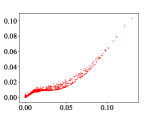
(a) synthetic, $\ell=1$

(b) synthetic, $\ell=2$

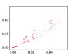
(c) synthetic, $\ell=3$

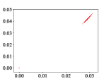
(d) synthetic, $\ell=4$

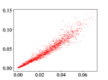
(e) mini-imagenet, $\ell=1$

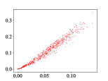
(f) mini-imagenet, $\ell=2$

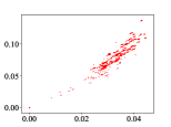
(g) mini-imagenet, $\ell=3$

(h) mini-imagenet, $\ell=4$

Figure 1: Property of optimal solution for $L=4$ hidden-layer fully connected NN. The top (synthetic 1-d regression) and bottom (mini-imagenet) rows are scatter-plots of the estimated quantities for each sampled neuron after convergence. For each subplot, one point $(x,y)$ represents one sampled neuron $j\in[m^{(\ell)}]$, where $x=u_{\_}j^{(\ell)}$ and $y=v_{\_}j^{(\ell)}$ defined in (6.1) and (6.2) respectively.

6.2 Synthetic 1-D regression task

We begin to empirically validate our claims in a synthetic 1-D regression task. Since the feature representation $f^{(\ell)}_{\_}j(x)$ corresponding to each neuron in each layer $\ell\in[L]$ is a single-variable function, it can be easily visualized.

Here we consider the function $f(x)=2(2\cos^{2}(x)-1)^{2}-1$ introduced by Mhaskar et al., (2017). We draw 60k training samples and 60k test samples uniformly from $[-2\pi,2\pi]$ for $x$ and set $y=f(x)$. We use a fully-connected NN with $m^{(\ell)}=1000\times 2^{L-\ell}$ hidden units in each hidden layer $\ell$ to learn this target function. We take $L=\{1,\cdots,4\}$, and use the Adam optimizer with an initial learning rate $1e$-$4$ in our experiments, and let the activation function be $\sigma(x)=\text{tanh}(x)$. For fair comparison, we tune the hyper-parameters of the weight of regularizer so that for different $L$, the NN could reach training RMSE of $1e$-$4$ when converge. This controls the representation power of the NN.

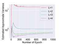
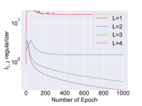
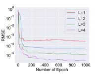
Figure 2: The visualization of optimization process when training multilayer NNs with different $L$.

We first validate that fully trained overparameterized NN satisfies the optimality condition of Corollary 7. Here we consider the case of $L=4$, and the top row in Fig 1 plots the estimated quantities $u_{\_}j^{(\ell)}$ and $v_{\_}j^{(\ell)}$. We can see that these two quantities are approximately linearly correlated, as predicted by Corollary 7.

To compare the performance of shallow versus deep networks, Fig 2 (a) reports how does the approximated variance change when $L$ increases. It demonstrates that the approximated variance decreases as $L$ increases. Moreover, the approximate variance gap between $L=2$ and $L=3$ is very large while that between $L=3$ and $L=4$ is small. This is consistent with the fact that the hierarchical composition of the target function $f(x)$ has depth $3$ (i.e. $f(x)=h(h(\cos x))$, where $h(u)=u^{2}-1$). At the same time, we can observe that for larger $L$, the regularizer in subplot (b) and training RMSE in subplot (c) decrease much faster, which also demonstrate the effectiveness of increasing $L$ for this target function.

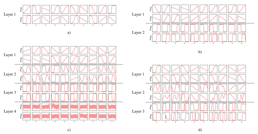
Figure 3: Representative features as 1-D functions for fully-connected NNs with different hidden-layers: a) 1-hidden-layer b) 2-hidden-layers c) 3-hidden-layers d) 4-hidden-layers. For each architecture, we sample 20 neurons from each layer and plot the single-variable feature function $f^{(\ell)}_{\_}j(x)$ of the sampled neurons.

Fig 3 shows representative features (as 1D-functions) at each layer after convergence. We reach the following conclusion from visualization of different $L$: DNN is able to learn hierarchical feature representations when we take optimization process into consideration. To be more specific, the layer next to the input layer tends to learn low-frequency signals while the upper layers take these lower-frequency signals to form higher-frequency signals.

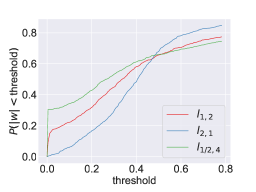
(a) weights of $w^{(1)}$

(b) weights of $w^{(2)}$

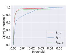
(c) weights of $w^{(3)}$

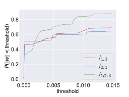
(d) weights of $u$

Figure 4: The comparison of sparsity of weights in different layers between different regularizers. The $i$-th figure demonstrate the sparsity of weights in $i$-th layer for different regularizers. The point $(x,y)$ on one curve suggests that there are $100\times y\%$ weights in such layer lies in $[-x,x]$. We could see that the red curve is lower-bounded by the blue one, which suggests that our proposed regularizer will result in more sparse representations compared with traditional regularizer.

We further compare the compactness of different regularizers. Here we use the notation $\ell_{\_}{a,b}$ to represent the regularizer in the form of $r_{\_}1(x)=|x|^{a}$ and $r_{\_}2(x)=|x|^{b}$. $\ell_{\_}{1,2}$ regularizer is the proposed regularizer, which is an upper-bound of the approximation variance. $\ell_{\_}{2,1}$ regularizer is the traditional $L_{\_}2$ regularizer (i.e. $\ell_{\_}2$ weight decay). From Fig 4, we found that the proposed regularizer leads to sparser weights, and thus has a more compact representation. We have also tried the $\ell_{\_}{1/2,4}$ regularizer, and found that the sparsity of $\ell_{\_}{1/2,4}$ regularizer isn’t significantly better than the proposed $\ell_{\_}{1,2}$ regularizer. This verifies the effectiveness of the proposed regularizer to obtain sparse weights.

Finally, we show that the proposed discrete feature repopulation (DFR) process can reduce the training loss, especially the regularizer loss (in Fig 6 (b)). This implies that it leads to a better feature representation. In our implementation, we first use Proximal Gradient Descent to optimize the objective (3.7) with respect to to the variables $\{\{p_{\_}j^{(\ell)}\}_{\_}{j=1}^{m^{(\ell)}}\}_{\_}{\ell=1}^{L}$ under the constraints that $\sum_{\_}{j=1}^{m^{(\ell)}}p_{\_}j^{(\ell)}=1$ for $\ell\in[L]$. When these repopulation weights $\{\{p_{\_}j^{(\ell)}\}_{\_}{j=1}^{m^{(\ell)}}\}_{\_}{\ell=1}^{L}$ are calculated, we use the algorithm described in Section 6.1 to discretely re-sample useful features from top layer to bottom layer. Fig 5 is a comparison of learned feature functions between vanilla SGD and SGD with DFR process described above. The feature functions learned by vanilla SGD contains some useless feature functions whose variance with respect to input $x$ is near zero, while the DFR process is able to remove these bad feature functions since their importance weights are relatively low. The difference is highly visible in Layer 3.

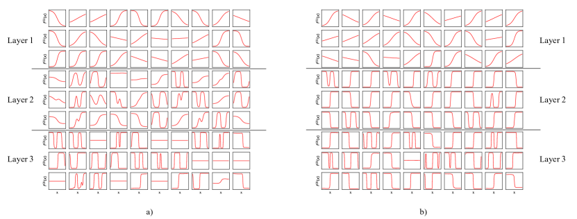
Figure 5: Representative feature functions of a) SGD without DFR b) SGD with one DFR process every 10 epochs during the first 50 epochs and every 100 epochs after epoch 50. In each subplot, we sample 30 neurons from each layer and plot the single-variable feature function $f^{(\ell)}_{\_}j(x)$ of sampled neurons.

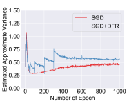
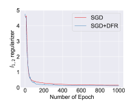
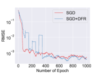
Figure 6: The comparison of optimization process between SGD and SGD with DFR for 3-hidden-layer NN.

6.3 Mini-Imagenet classification task

We have also performed experiments on real data. Mini-Imagenet dataset is a simplified version of ILSVRC’12 dataset (Russakovsky et al.,, 2015), which consists of 600 84$\times$84$\times$3 images sampled from 100 classes each. Here we consider the data split introduced by (Ravi & Larochelle,, 2016), which consists of 64 classes and 38.4k images as our full dataset. We divide the dataset into train/valid/test split by 7:1:2.

Since fully-connected NNs do not have the capacity to deal with such image data, we first train a base CNN embedding network with a four block architecture as in (Vinyals et al.,, 2016). We then take the $1600$-dimensional output of the embedding layer and feed it to an $L$ layer NN for classification. The training configurations and network architectures are the same as those for the synthetic 1-D experiment, except that we tune the regularization parameters to achieve the best validation accuracy. Since the feature function of this task is hard to visualize, we only consider the optimality condition, shallow versus deep networks and compactness.

Similar to the results in the synthetic 1-D experiment, the sub-figures in the bottom row of Fig 1 show that the two quantities we care about are also linearly correlated in each layer, which is consistent with our theory. Fig 7 reports how approximation variance, test RMSE, and train RMSE change during the model training procedure. We can see that the approximation variance decreases as $L$ increases, and the gap between $L=1$ and $L=2$ is very large. This demonstrates the great advantage of deeper networks. Moreover, the generalization performance also increases as $L$ increases.

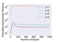
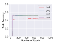
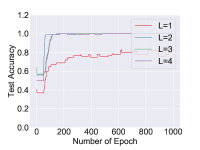
Figure 7: Visualization of the optimization process when training multilayer NNs with different $L$.

Fig 8 shows that the proposed $\ell_{\_}{1,2}$ regularizer leads to more compact weights for each layer than the traditional $\ell_{\_}{2,1}$. .

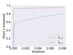
(a) weights of $w^{(1)}$

(b) weights of $w^{(2)}$

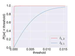
(c) weights of $w^{(3)}$

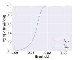
(d) weights of $u$

Figure 8: Comparison of weight sparsity at different layers for different regularizers on the Mini-Imagenet classification task. The $i$-th figure demonstrates the weight sparsity at layer $i$ for different regularizers. A point $(x,y)$ indicates that there are $100\times y\%$ weight values lying in $[-x,x]$. We can see that the red curve dominates the blue one, which suggests that the proposed regularizer leads to sparser solutions than those of the traditional $\ell_{\_}2$ regularizer.

7 Conclusion

This paper introduced the NFR technique to analyze over-parameterized DNNs and showed that it is possible to reformulate overparameterized DNNs as convex systems. Moreover, when fully trained, DNNs learn effective feature representations suitable for the underlying learning task via regularization. Our analysis is consistent with empirical observations.

Similar to the analysis of two-level NN in (Fang et al., 2019a, ), this newly introduced NFR method paves the way for establishing global convergence results of standard optimization algorithms such as (noisy) gradient descent for overparameterized DNNs. We will leave such study as a future work.

Acknowledgement

The authors would like to thank Jason Lee, Xiang Wang, and Pengkun Yang for very helpful discussions.

Appendix A Preliminary

This section provides some useful known inequalities that will be later used in our proofs.

A.1 Jensen’s Inequality

In our proof, we will frequently use the Jensen’s inequality, which relates the value of a convex function of an integral to the integral of the convex function. In probability theory, it states that if $\phi$ is a convex function, for a random variable $x$, we have

$$\phi\left(\mathbb{E}[x]\right)\leq\mathbb{E}[\phi(x)].$$

We are particularly interested in the case when $\phi(x)=|x|^{p}$ where $p\geq 1$. We can obtain

$$|\mathbb{E}[x]|\leq(\mathbb{E}[|x|^{p}])^{1/p},\quad p\geq 1.$$

In the finite form, Jensen’s inequality takes the form of:

$$\phi\left(\frac{1}{n}\sum_{\_}{i=1}^{n}x_{\_}i\right)\leq\frac{1}{n}\sum_{\_}{i=1}^{n}\phi(x_{\_}i).$$ (A.1)

If we further assume $x_{\_}i$ with $i\in[n]$ are independent random variables which follow from a same underlying distribution, by taking expectation on (A.1), we have

$$\mathbb{E}\left[\phi\left(\frac{1}{n}\sum_{\_}{i=1}^{n}x_{\_}i\right)\right]\leq\frac{1}{n}\sum_{\_}{i=1}^{n}\mathbb{E}[\phi(x_{\_}i)]=\mathbb{E}[\phi(x_{\_}1)].$$ (A.2)

A.2 Rosenthal Inequality

We will also use the Rosenthal Inequality to build relations between moments of a collection of independent random variables. It is stated in the following:

Lemma 1 (Rosenthal Inequality (Ibragimov & Sharakhmetov,, 1999)).

Let $\xi_{\_}i$ with $i\in[n]$ be independent with $\mathbb{E}[\xi_{\_}i]=0$ and $\mathbb{E}[|\xi_{\_}i|^{t}]<\infty$ for some $t\geq 2$. Then we have

$$\mathbb{E}\left|\sum_{\_}{i=1}^{n}\xi_{\_}i\right|^{t}\leq C^{1}_{\_}t\left(\sum_{\_}{i=1}^{n}\mathbb{E}|\xi_{\_}i|^{t}\right)+C^{2}_{\_}t\left(\sum_{\_}{i=1}^{n}\mathbb{E}[\xi_{\_}i^{2}]\right)^{t/2},$$

where $C^{1}_{\_}t$ can be token as $(ct)^{t}$, $C^{2}_{\_}t=(c\sqrt{t})^{t}$, and $c$ is a constant.

Appendix B Proof of Theorem 1: Consistency of Discretization

In this section, we prove Theorem 1 which shows the discrete DNN converges to the corresponding continuous one in $L^{1}$. Before giving the detailed proof, we give the following definitions.

• We denote $\mathcal{I}^{(\ell)}$ to be the set consisting of all ordered sequences in the form of $\{k_{\_}1,k_{\_}2,\dots,k_{\_}{\ell}\}$ with $k_{\_}{j}\in[m^{(j)}]$ and $j\in[\ell]$. That is

  $$\mathcal{I}^{(\ell)}:=[m^{(1)}]\otimes[m^{(2)}]\otimes\cdots\otimes[m^{(\ell)}],$$

  where $\otimes$ means the Cartesian product.

• We denote $\hat{\mathcal{Z}}^{(\ell)}:=\{z^{(\ell)}_{\_}{j}:~{}j\in[m^{(\ell)}]\}$, and let

  $$\{z\}_{\_}{\mathcal{I}^{(\ell)}}:=\hat{\mathcal{Z}}^{(1)}\cup\cdots\cup\hat{\mathcal{Z}}^{(\ell)}.$$

• $\mathbb{E}[f]$ means taking full expectation on all the random variables. $\mathbb{E}_{\_}{\hat{\mathcal{Z}}^{(\ell)}}[f]$ (or $\mathbb{E}_{\_}{\{z\}_{\_}{\mathcal{I}^{(\ell)}}}[f]$) stands for taking the (conditional) expectation on $\hat{\mathcal{Z}}^{(\ell)}$ (or $\{z\}_{\_}{\mathcal{I}^{(\ell)}}$).

• We define

  $$\Delta^{(\ell)}\big{(}z^{(\ell)}\big{)}:=\left|\frac{1}{m^{(\ell-1)}}\sum_{\_}{j=1}^{m^{(\ell-1)}}w(z^{(\ell)},z^{(\ell-1)}_{\_}j)f^{(\ell-1)}(\rho,z^{(\ell-1)}_{\_}j;x)-g^{(\ell)}(\rho,z^{(\ell)};x)\right|,\quad\ell\in[L+1],$$

  and

  $$\Delta^{(L+1)}\big{(}z^{(L+1)}\big{)}:=\left\|\frac{1}{m^{(L)}}\sum_{\_}{j=1}^{m^{(L)}}u(z^{(L)}_{\_}j)f^{(L)}(\rho,z^{(L)}_{\_}j;x)-f(\rho,u;x)\right\|,$$

  where we denote $z^{(L+1)}=1$. Clearly, we have $\Delta^{(1)}\big{(}z^{(1)}\big{)}=0$.

• We define

  $$A(k,L+1):=\begin{cases}1,&k=L+1,\\ \left\|u(z^{(L)})\right\|,&k=L,\\ \left\|u(z^{(L)})\right\|\prod_{\_}{j=k+1}^{L}|w(z^{(j)},z^{(j-1)})|,&k\in[L-1],\\ \end{cases}$$

  and for $\ell\in\{2,\dots,L\}$, we define

  $$A(k,\ell):=\begin{cases}1,&k=\ell,\\ \prod_{\_}{j=k+1}^{\ell}|w(z^{(j)},z^{(j-1)})|,&k<\ell.\\ \end{cases}$$

• We define

  $$\bar{f}^{(\ell)}(z^{(\ell)};x)=h^{(\ell)}\Big{(}\frac{1}{m^{(\ell-1)}}\sum_{\_}{j=1}^{m^{(\ell-1)}}w(z^{(\ell)},z^{(\ell-1)}_{\_}j)\hat{f}^{(\ell-1)}_{\_}j(x)\Big{)},\quad\ell\in[L].$$

  It holds that $\bar{f}^{(\ell)}(z^{(\ell)}_{\_}j;x)=\hat{f}^{(\ell)}_{\_}j(x)$ for all $\ell\in[L]$ and $j\in[m^{(\ell)}]$. We note that $\Delta^{(\ell)}(z^{(\ell)})$ depends on random variables in $\hat{\mathcal{Z}}^{(\ell-1)}$ and $\bar{f}^{(\ell)}(z^{(\ell)};x)$ depends on the random variables in $\hat{\mathcal{Z}}^{(1)},\dots,\hat{\mathcal{Z}}^{(\ell-1)}$.

Now we begin our proof.

Step 1. We prove for all $\ell\in\{2,\dots,L\}$,

$$\!\!\!\!\mathbb{E}_{\_}{z^{(\ell)}}\mathbb{E}_{\_}{\{z\}_{\_}{\mathcal{I}^{(\ell-1)}}}\left|\bar{f}^{(\ell)}(z^{(\ell)};x)-f^{(\ell)}(\rho,z^{(\ell)};x)\right|\!\leq\!\sum_{\_}{j=2}^{\ell}(c_{\_}0)^{\ell-j+1}\mathbb{E}_{\_}{z^{(j)},\dots,z^{(\ell)}}\mathbb{E}_{\_}{\hat{\mathcal{Z}}^{(j-1)}}A(j,\ell)\Delta^{(j)}(z^{(j)}).$$ (B.1)

In the inequalities above $\mathbb{E}_{\_}{z^{(j)},\dots,z^{(\ell-1)}}\mathbb{E}_{\_}{\hat{\mathcal{Z}}^{(j-1)}}$ means $\mathbb{E}_{\_}{\hat{\mathcal{Z}}^{(j-1)}}$ when $j=\ell$, i.e., we only take expectation on $\hat{\mathcal{Z}}^{(j-1)}$. Moreover, we have

$$\mathbb{E}_{\_}{\{z\}_{\_}{\mathcal{I}^{(L)}}}\left\|\hat{f}(x)-f(\rho,u,x)\right\|\leq\sum_{\_}{j=2}^{\ell}(c_{\_}0)^{\ell-j+1}\mathbb{E}_{\_}{z^{(j)},\dots,z^{(\ell-1)}}\mathbb{E}_{\_}{\hat{\mathcal{Z}}^{(j-1)}}A(j,\ell)\Delta^{(j)}(z^{(j)}).$$ (B.2)

Proof.

For all $\ell\in[L]$ and $k\in[\ell]$, we have

$$\mathbb{E}_{\_}{\{z\}_{\_}{\mathcal{I}^{(k-1)}}}A(k,\ell)\left|\bar{f}^{(k)}(z^{(k)};x)-f^{(k)}(\rho,z^{(k)};x)\right|$$ (B.3)

$$= \mathbb{E}_{\_}{\{z\}_{\_}{\mathcal{I}^{(k-1)}}}A(k,\ell)\Bigg{|}h^{(k)}\Big{(}\frac{1}{m^{(k-1)}}\sum_{\_}{j=1}^{m^{(k-1)}}w(z^{(k)},z^{(k-1)}_{\_}j)\hat{f}^{(k-1)}_{\_}j(x)\Big{)}$$

$$\quad\quad\quad\quad\quad\quad\quad\quad\quad\quad\quad\quad\quad\quad\quad\quad\quad\quad~{}~{}~{}-h^{(k)}\Big{(}\mathbb{E}_{\_}{z^{(k-1)}}\left[w(z^{(k)},z^{(k-1)})f^{(k-1)}(\rho,z^{(k-1)};x)\right]\Big{)}\Bigg{|}$$

$$\overset{a}{\leq} c_{\_}0\mathbb{E}_{\_}{\{z\}_{\_}{\mathcal{I}^{(k-1)}}}A(k,\ell)\Bigg{|}\underbrace{\frac{1}{m^{(k-1)}}\sum_{\_}{j=1}^{m^{(k-1)}}\left[w(z^{(k)},z^{(k-1)}_{\_}j)\hat{f}^{(k-1)}_{\_}j(x)\right]}_{\_}{=a_{\_}1}$$

$$\quad\quad\quad\quad\quad\quad\quad\quad\quad\quad\quad\quad\quad\quad\quad\quad\quad\quad\quad\quad\quad~{}~{}-\underbrace{\mathbb{E}_{\_}{z^{(k-1)}}\left[w(z^{(k)},z^{(k-1)})f^{(k-1)}(\rho,z^{(k-1)};x)\right]}_{\_}{=g^{k}(\rho,z^{(k)};x)=b_{\_}1}\Bigg{|}$$

$$\overset{b}{\leq} c_{\_}0\mathbb{E}_{\_}{\{z\}_{\_}{\mathcal{I}^{(k-1)}}}A(k,\ell)\Bigg{|}\underbrace{\frac{1}{m^{(k-1)}}\sum_{\_}{j=1}^{m^{(k-1)}}w(z^{(k)},z^{(k-1)}_{\_}j)f^{(k-1)}(\rho,z^{(k-1)}_{\_}j;x)}_{\_}{=c_{\_}1}-g^{(k)}(\rho,z^{(k)};x)\Bigg{|}$$

$$\quad\quad\quad\quad~{}~{}~{}+c_{\_}0\mathbb{E}_{\_}{\{z\}_{\_}{\mathcal{I}^{(k-1)}}}A(k,\ell)\Bigg{|}\underline{\frac{1}{m^{(k-1)}}\sum_{\_}{j=1}^{m^{(k-1)}}}w(z^{(k)},z^{(k-1)}_{\_}j)\left[\underline{\hat{f}^{(k-1)}_{\_}j(x)}-f^{(k-1)}(\rho,z^{(k-1)}_{\_}j;x)\right]\Bigg{|}$$

$$\leq c_{\_}0\mathbb{E}_{\_}{\{z\}_{\_}{\mathcal{I}^{(k-1)}}}A(k,\ell)\Bigg{|}\frac{1}{m^{(k-1)}}\sum_{\_}{j=1}^{m^{(k-1)}}w(z^{(k)},z^{(k-1)}_{\_}j)f^{(k-1)}(\rho,z^{(k-1)}_{\_}j;x)-g^{(k)}(\rho,z^{(k)};x)\Bigg{|}$$

$$\quad\quad~{}+c_{\_}0\mathbb{E}_{\_}{\{z\}_{\_}{\mathcal{I}^{(k-1)}}}A(k,\ell)\underline{\frac{1}{m^{(k-1)}}\sum_{\_}{j=1}^{m^{(k-1)}}}\Bigg{|}w(z^{(k)},z^{(k-1)}_{\_}j)\left[\underline{\bar{f}^{(k-1)}(z^{(k-1)}_{\_}j;x)}-f^{(k-1)}(\rho,z^{(k-1)}_{\_}j;x)\right]\Bigg{|}$$

$$\overset{c}{=} c_{\_}0\mathbb{E}_{\_}{\{z\}_{\_}{\mathcal{I}^{(k-1)}}}A(k,\ell)\Delta^{(k)}(z^{(k)})$$

$$\quad\quad\quad\quad\quad~{}+c_{\_}0\mathbb{E}_{\_}{z^{(k-1)}}\mathbb{E}_{\_}{\{z\}_{\_}{\mathcal{I}^{(k-2)}}}A(k,\ell)\Bigg{|}w(z^{(k)},z^{(k-1)})\left[\bar{f}^{(k-1)}(z^{(k-1)};x)-f^{(k-1)}(\rho,z^{(k-1)};x)\right]\Bigg{|}$$

$$\overset{d}{=} c_{\_}0\mathbb{E}_{\_}{\hat{\mathcal{Z}}^{(k-1)}}A(k,\ell)\Delta^{(k)}(z^{(k)})+c_{\_}0\mathbb{E}_{\_}{z^{(k-1)}}\mathbb{E}_{\_}{\{z\}_{\_}{\mathcal{I}^{(k-2)}}}A(k-1,\ell)\Bigg{|}\bar{f}^{(k-1)}(z^{(k-1)};x)-f^{(k-1)}(\rho,z^{(k-1)};x)\Bigg{|},$$

where $\overset{a}{\leq}$ we use Assumption 1 and obtain the result by mean value theorem, $\overset{b}{\leq}$ uses triangle inequality, i.e., $|a_{\_}1-b_{\_}1|\leq|c_{\_}1-b_{\_}1|+|a_{\_}1-c_{\_}1|$, in $\overset{c}{=}$, we take conditional expectation on $\hat{\mathcal{Z}}^{(k-1)}$ for the second term, and in $\overset{d}{=}$, we use the fact that $\Delta^{(k)}(z^{(k)})$ only depends on random variables $\hat{\mathcal{Z}}^{(k-1)}$. Thus for all $\ell\in[L]$, we have

$$\mathbb{E}_{\_}{\{z\}_{\_}{\mathcal{I}^{(\ell-1)}}}\left|\bar{f}^{(\ell)}(z^{(\ell)};x)-f^{(\ell)}(\rho,z^{(\ell)};x)\right|$$ (B.4)

$$= \mathbb{E}_{\_}{\{z\}_{\_}{\mathcal{I}^{(\ell-1)}}}A(\ell,\ell)\left|\bar{f}^{(\ell)}(z^{(\ell)};x)-f^{(\ell)}(\rho,z^{(\ell)};x)\right|$$

$$\overset{\eqref{the1:a1}}{\leq} c_{\_}0\mathbb{E}_{\_}{\hat{\mathcal{Z}}^{(\ell-1)}}A(\ell,\ell)\Delta^{(\ell)}(z^{(\ell)})+c_{\_}0\mathbb{E}_{\_}{z^{(\ell-1)}}\underbrace{\mathbb{E}_{\_}{\{z\}_{\_}{\mathcal{I}^{(\ell-2)}}}A(\ell-1,\ell)\Bigg{|}\bar{f}^{(\ell-1)}(z^{(\ell)};x)-f^{(\ell-1)}(\rho,z^{(\ell-1)};x)\Bigg{|}}_{\_}{\eqref{the1:a1}}$$

$$\leq \ldots$$

$$\vdots$$

$$\leq \sum_{\_}{j=1}^{\ell}(c_{\_}0)^{\ell-j+1}\mathbb{E}_{\_}{z^{(j)},\dots,z^{(\ell-1)}}\mathbb{E}_{\_}{\hat{\mathcal{Z}}^{(j-1)}}A(j,\ell)\Delta^{(j)}(z^{(j)})+(c_{\_}0)^{\ell}\mathbb{E}_{\_}{z^{1},\dots,z^{\ell-1}}\underbrace{\mathbb{E}_{\_}{\hat{\mathcal{Z}}^{(0)}}\Bigg{|}\bar{f}^{(1)}(z^{(1)};x)-f^{(1)}(\rho,z^{(1)};x)\Bigg{|}}_{\_}{0}$$

$$\overset{a}{=} \sum_{\_}{j=2}^{\ell}(c_{\_}0)^{\ell-j+1}\mathbb{E}_{\_}{z^{(j)},\dots,z^{(\ell-1)}}\mathbb{E}_{\_}{\hat{\mathcal{Z}}^{(j-1)}}A(j,\ell)\Delta^{(j)}(z^{(j)}),$$

where in $\overset{a}{=}$ we use $\Delta^{(1)}\big{(}z^{(1)}\big{)}=0$.

We consider the top layer. In fact, using the same technique in (B.3), we have

$$\mathbb{E}_{\_}{\{z\}_{\_}{\mathcal{I}^{(L)}}}\left\|\hat{f}(x)-f(\rho,u,x)\right\|$$ (B.5)

$$= \mathbb{E}_{\_}{\{z\}_{\_}{\mathcal{I}^{(L)}}}\left\|\frac{1}{m^{(L)}}\sum_{\_}{j=1}^{m^{(L)}}u^{(L)}_{\_}j\bar{f}^{(L)}(z^{(L)}_{\_}j;x)-\mathbb{E}_{\_}{z^{(L)}}\left[u^{(L)}f^{(L)}(\rho,z^{(L)};x)\right]\right\|$$

$$\leq \mathbb{E}_{\_}{\{z\}_{\_}{\mathcal{I}^{(L)}}}\left\|\frac{1}{m^{(L)}}\sum_{\_}{j=1}^{m^{(L)}}u^{(L)}_{\_}j\left[\bar{f}^{(L)}(z^{(L)}_{\_}j;x)-f^{(L)}(\rho,z^{(L)}_{\_}j;x)\right]\right\|$$

$$\quad\quad\quad\quad\quad\quad\quad\quad\quad\quad\quad~{}~{}+\mathbb{E}_{\_}{\{z\}_{\_}{\mathcal{I}^{(L)}}}\left\|\frac{1}{m^{(L)}}\sum_{\_}{j=1}^{m^{(L)}}u^{(L)}_{\_}jf^{(L)}(z^{(L)}_{\_}j;x)-\mathbb{E}_{\_}{z^{(L)}}\left[u^{(L)}f^{(L)}(\rho,z^{(L)};x)\right]\right\|$$

$$\overset{a}{\leq} \mathbb{E}_{\_}{z^{(L)}}\underbrace{\mathbb{E}_{\_}{\{z\}_{\_}{\mathcal{I}^{(L-1)}}}\left\|u^{(L)}\right\|\left|\bar{f}^{(L)}(z^{(L)};x)-f^{(L)}(\rho,z^{(L)};x)\right|}_{\_}{\eqref{theo1:a2}\text{ with }\ell=L}$$

$$\quad\quad\quad\quad\quad\quad\quad\quad\quad\quad\quad~{}~{}+\mathbb{E}_{\_}{\{z\}_{\_}{\mathcal{I}^{(L)}}}\left\|\frac{1}{m^{(L)}}\sum_{\_}{j=1}^{m^{(L)}}u^{(L)}_{\_}jf^{(L)}(z^{(L)}_{\_}j;x)-\mathbb{E}_{\_}{z^{(L)}}\left[u^{(L)}f^{(L)}(\rho,z^{(L)};x)\right]\right\|$$

$$\leq \sum_{\_}{j=2}^{L+1}(c_{\_}0)^{L-j+1}\mathbb{E}_{\_}{z^{(j)},\dots,z^{(L)}}\mathbb{E}_{\_}{\hat{\mathcal{Z}}^{(j-1)}}A(j,L+1)\Delta^{(j)}(z^{(j)}),$$

where $\overset{a}{\leq}$ is obtained by

$$\mathbb{E}_{\_}{\{z\}_{\_}{\mathcal{I}^{(L)}}}\left\|\frac{1}{m^{(L)}}\sum_{\_}{j=1}^{m^{(L)}}u^{(L)}_{\_}j\left[\bar{f}^{(L)}(z^{(L)}_{\_}j;x)-f^{(L)}(\rho,z^{(L)}_{\_}j;x)\right]\right\|$$

$$\leq \mathbb{E}_{\_}{\{z\}_{\_}{\mathcal{I}^{(L)}}}\frac{1}{m^{(L)}}\sum_{\_}{j=1}^{m^{(L)}}\left\|u^{(L)}_{\_}j\left[\bar{f}^{(L)}(z^{(L)}_{\_}j;x)-f^{(L)}(\rho,z^{(L)}_{\_}j;x)\right]\right\|$$

$$= \mathbb{E}_{\_}{z^{(L)}}\mathbb{E}_{\_}{\{z\}_{\_}{\mathcal{I}^{(L-1)}}}\left\|u^{(L)}\left[\bar{f}^{(L)}(z^{(L)};x)-f^{(L)}(\rho,z^{(L)};x)\right]\right\|$$

$$\leq \mathbb{E}_{\_}{z^{(L)}}\mathbb{E}_{\_}{\{z\}_{\_}{\mathcal{I}^{(L-1)}}}\left\|u^{(L)}\right\|\left|\bar{f}^{(L)}(z^{(L)};x)-f^{(L)}(\rho,z^{(L)};x)\right|.$$

We obtain (B.2). On the other hand, taking expectation on $z^{(\ell)}$ for (B.4), we can obtain (B.1). ∎

Step 2. We prove for all $\ell\in\{2,\dots,L\}$ and $j\in\{2,\dots,\ell\}$, we have

$$\lim_{\_}{m^{(j-1)}\to\infty}\mathbb{E}_{\_}{z^{(j)},\dots,z^{(\ell)}}\mathbb{E}_{\_}{\hat{\mathcal{Z}}^{(j-1)}}A(j,\ell)\Delta^{(j)}(z^{(j)})=0.$$ (B.6)

For all $j\in\{2,\dots,L+1\}$,

$$\lim_{\_}{m^{(j-1)}\to\infty}\mathbb{E}_{\_}{z^{(j)},\dots,z^{(L)}}\mathbb{E}_{\_}{\hat{\mathcal{Z}}^{(j-1)}}A(j,L+1)\Delta^{(j)}(z^{(j)})=0..$$ (B.7)

Note that when $j=L+1$, $\Delta(z^{(L+1)})$ is vector and the expectation is only taken on $\hat{\mathcal{Z}}^{(L)}$.

Proof.

We denote

$$Q{(\ell)}:=\begin{cases}1,&\ell=L+1,\\ \left(\|u^{(L)}(z^{(L)})\|\vee 1]\right)\prod_{\_}{i=\ell+1}^{L}\left(|w(z^{(i)},z^{(i-1)})|\vee 1\right),&\ell\in[L].\end{cases}$$

In fact, for all $\ell\in\{2,\dots,L\}$ and $j\in\{2,\dots,\ell\}$, we have

$$\mathbb{E}_{\_}{z^{(j)},\dots,z^{(\ell)}}\mathbb{E}_{\_}{\hat{\mathcal{Z}}^{(j-1)}}A(j,\ell)\Delta^{(j)}(z^{(j)})\leq\mathbb{E}_{\_}{z^{(j)},\dots,z^{(L)}}\mathbb{E}_{\_}{\hat{\mathcal{Z}}^{(j-1)}}Q{(j)}\Delta^{(j)}(z^{(j)}).$$ (B.8)

It is also true that all for $j\in[L+1]$,

$$\mathbb{E}_{\_}{z^{(j)},\dots,z^{(L)}}\mathbb{E}_{\_}{\hat{\mathcal{Z}}^{(j-1)}}A(j,L+1)\Delta^{(j)}(z^{(j)})\leq\mathbb{E}_{\_}{z^{(j)},\dots,z^{(L)}}\mathbb{E}_{\_}{\hat{\mathcal{Z}}^{(j-1)}}Q{(j)}\Delta^{(j)}(z^{(j)}).$$ (B.9)

In the following, we denote

$$\xi^{(j)}_{\_}k:=\begin{cases}Q(j)\left[w(z^{(j)},z^{(j-1)}_{\_}k)f^{(j-1)}(\rho,z^{(j-1)}_{\_}k;x)-g^{(j)}(\rho,z^{(j)};x)\right],&j\in\{2,\dots,L\},~{}~{}k\in[m^{(j-1)}],\\ u(z^{(L)}_{\_}k)f^{(L)}(\rho,z^{(L)}_{\_}k;x)-f(\rho,u;x),&j=L+1,~{}~{}k\in[m^{(L)}].\end{cases}$$

Note that $\xi^{(L+1)}_{\_}k$ with $k\in[m^{(L)}]$ are $K$ dimensional vectors. Because the real numbers can also be treated as one dimensional vectors. Below we treat $\xi^{(j)}_{\_}k$ as a vector for the sake of simplicity. We have for all $j\in\{2,\dots,L+1\}$

$$\mathbb{E}_{\_}{z^{(j)},\dots,z^{(L)}}\mathbb{E}_{\_}{\hat{\mathcal{Z}}^{(j-1)}}Q{(j)}\Delta^{(j)}(z^{(j)})$$ (B.10)

$$= \mathbb{E}_{\_}{z^{(j)},\dots,z^{(L)}}\mathbb{E}_{\_}{\hat{\mathcal{Z}}^{(j-1)}}\left\|\frac{1}{m^{(j-1)}}\sum_{\_}{k=1}^{m^{(j-1)}}\xi^{(j)}_{\_}k\right\|$$

$$\overset{a}{\leq} \mathbb{E}_{\_}{z^{(j)},\dots,z^{(L)}}\mathbb{E}_{\_}{\hat{\mathcal{Z}}^{(j-1)}}\left\|\frac{1}{m^{(j-1)}}\sum_{\_}{k=1}^{m^{(j-1)}}\xi^{(j)}_{\_}k\mathbf{1}_{\_}{\|\xi^{(j)}_{\_}k\|\leq M}\right\|+\mathbb{E}_{\_}{z^{(j)},\dots,z^{(L)}}\mathbb{E}_{\_}{\hat{\mathcal{Z}}^{(j-1)}}\left\|\frac{1}{m^{(j-1)}}\sum_{\_}{k=1}^{m^{(j-1)}}\xi^{(j)}_{\_}k\mathbf{1}_{\_}{\|\xi^{(j)}_{\_}k\|>M}\right\|$$

$$\overset{b}{\leq} \mathbb{E}_{\_}{z^{(j)},\dots,z^{(L)}}\sqrt{\mathbb{E}_{\_}{\hat{\mathcal{Z}}^{(j-1)}}\left\|\frac{1}{m^{(j-1)}}\sum_{\_}{k=1}^{m^{(j-1)}}\xi^{(j)}_{\_}k\mathbf{1}_{\_}{\|\xi^{(j)}_{\_}k\|\leq M}\right\|^{2}}+\mathbb{E}_{\_}{z^{(j)},\dots,z^{(L)}}\mathbb{E}_{\_}{\hat{\mathcal{Z}}^{(j-1)}}\frac{1}{m^{(j-1)}}\sum_{\_}{k=1}^{m^{(j-1)}}\left\|\xi^{(j)}_{\_}k\mathbf{1}_{\_}{\|\xi^{(j)}_{\_}k\|>M}\right\|$$

$$\leq \mathbb{E}_{\_}{z^{(j)},\dots,z^{(L)}}\sqrt{\mathbb{E}_{\_}{\hat{\mathcal{Z}}^{(j-1)}}\left\|\frac{1}{m^{(j-1)}}\sum_{\_}{k=1}^{m^{(j-1)}}\xi^{(j)}_{\_}k\mathbf{1}_{\_}{\|\xi^{(j)}_{\_}k\|\leq M}\right\|^{2}}+\mathbb{E}_{\_}{z^{(j)},\dots,z^{(L)}}\mathbb{E}_{\_}{z^{(j-1)}_{\_}1}\left\|\xi^{(j)}_{\_}1\mathbf{1}_{\_}{\|\xi^{(j)}_{\_}1\|>M}\right\|,$$

where in $\overset{a}{=}$, we use $\mathbf{1}$ to denote indicator function, then

$$\frac{1}{m^{(j-1)}}\sum_{\_}{k=1}^{m^{(j-1)}}\xi^{(j)}_{\_}k=\frac{1}{m^{(j-1)}}\sum_{\_}{k=1}^{m^{(j-1)}}\xi^{(j)}_{\_}k\mathbf{1}_{\_}{\|\xi^{(j)}_{\_}k\|\leq M}+\frac{1}{m^{(j-1)}}\sum_{\_}{k=1}^{m^{(j-1)}}\xi^{(j)}_{\_}k\mathbf{1}_{\_}{\|\xi^{(j)}_{\_}k\|>M},$$

and obtain the result by triangle inequality, and $\overset{b}{\leq}$ uses Jensen’s inequality. For the first term in the right hand side of (B.10), we have

$$\mathbb{E}_{\_}{z^{(j)},\dots,z^{(L)}}\sqrt{\mathbb{E}_{\_}{\hat{\mathcal{Z}}^{(j-1)}}\left\|\frac{1}{m^{(j-1)}}\sum_{\_}{k=1}^{m^{(j-1)}}\xi^{(j)}_{\_}k\mathbf{1}_{\_}{\|\xi^{(j)}_{\_}k\|\leq M}\right\|^{2}}$$ (B.11)

$$= \mathbb{E}_{\_}{z^{(j)},\dots,z^{(L)}}\Bigg{(}\frac{1}{(m^{(j-1)})^{2}}\sum_{\_}{k_{\_}1=1}^{m^{(j-1)}}\mathbb{E}_{\_}{z^{(j-1)}_{\_}{k_{\_}1}}\left\|\xi^{(j)}_{\_}{k_{\_}1}\mathbf{1}_{\_}{\|\xi^{(j)}_{\_}{k_{\_}1}\|\leq M}\right\|^{2}$$

$$\quad\quad\quad\quad\quad\quad\quad\quad+\frac{1}{(m^{(j-1)})^{2}}\sum_{\_}{k_{\_}1=1}^{m^{(j-1)}}\sum_{\_}{k_{\_}2=1,k_{\_}2\neq k_{\_}1}^{m^{(j-1)}}\mathbb{E}_{\_}{z^{(j-1)}_{\_}{k_{\_}1}}\mathbb{E}_{\_}{z^{(j-1)}_{\_}{k_{\_}2}}\left[\xi^{(j)}_{\_}{k_{\_}1}\mathbf{1}_{\_}{\|\xi^{(j)}_{\_}{k_{\_}1}\|\leq M}\right]^{\top}\left[\xi^{(j)}_{\_}{k_{\_}2}\mathbf{1}_{\_}{\|\xi^{(j)}_{\_}{k_{\_}2}\|\leq M}\right]\Bigg{)}^{1/2}$$

$$\overset{a}{=} \mathbb{E}_{\_}{z^{(j)},\dots,z^{(L)}}\sqrt{\frac{1}{(m^{(j-1)})}\mathbb{E}_{\_}{z^{(j-1)}_{\_}{1}}\left\|\xi^{(j)}_{\_}{1}\mathbf{1}_{\_}{\|\xi^{(j)}_{\_}1\|\leq M}\right\|^{2}+\frac{m^{(j-1)}-1}{m^{(j-1)}}\left\|\mathbb{E}_{\_}{z^{(j-1)}_{\_}{1}}\left[\xi^{(j)}_{\_}{1}\mathbf{1}_{\_}{\|\xi^{(j)}_{\_}1\|\leq M}\right]\right\|^{2}}$$

$$= \mathbb{E}_{\_}{z^{(j)},\dots,z^{(L)}}\sqrt{\frac{1}{(m^{(j-1)})}\mathbb{E}_{\_}{z^{(j-1)}_{\_}{1}}\left\|\xi^{(j)}_{\_}{1}\mathbf{1}_{\_}{\|\xi^{(j)}_{\_}1\|\leq M}\right\|^{2}+\underbrace{\frac{m^{(j-1)}-1}{m^{(j-1)}}}_{\_}{\leq 1}\underbrace{\left\|\mathbb{E}_{\_}{z^{(j-1)}_{\_}{1}}\left[\xi^{(j)}_{\_}1-\xi^{(j)}_{\_}1\mathbf{1}_{\_}{\|\xi^{(j)}_{\_}1\|>M}\right]\right\|^{2}}_{\_}{\mathbb{E}_{\_}{z^{(j-1)}_{\_}{1}}\xi_{\_}1^{j}=0}}$$

$$\leq \mathbb{E}_{\_}{z^{(j)},\dots,z^{(L)}}\sqrt{\frac{1}{(m^{(j-1)})}\mathbb{E}_{\_}{z^{(j-1)}_{\_}{1}}\left\|\xi^{(j)}_{\_}{1}\mathbf{1}_{\_}{\|\xi^{(j)}_{\_}1\|\leq M}\right\|^{2}+\left\|\mathbb{E}_{\_}{z^{(j-1)}_{\_}{1}}\left[\xi^{(j)}_{\_}1\mathbf{1}_{\_}{\|\xi^{(j)}_{\_}1\|>M}\right]\right\|^{2}}$$

$$\overset{b}{\leq} \frac{1}{\sqrt{m^{(j-1)}}}\mathbb{E}_{\_}{z^{(j)},\dots,z^{(L)}}\sqrt{\mathbb{E}_{\_}{z^{(j-1)}_{\_}{1}}\left\|\xi^{(j)}_{\_}{1}\mathbf{1}_{\_}{\|\xi^{(j)}_{\_}1\|\leq M}\right\|^{2}}+\mathbb{E}_{\_}{z^{(j)},\dots,z^{(L)}}\left\|\mathbb{E}_{\_}{z^{(j-1)}_{\_}{1}}\xi^{(j)}_{\_}1\mathbf{1}_{\_}{\|\xi^{(j)}_{\_}1\|>M}\right\|$$

$$\overset{c}{\leq} \frac{1}{\sqrt{m^{(j-1)}}}\sqrt{\mathbb{E}_{\_}{z^{(j)},\dots,z^{(L)}}\mathbb{E}_{\_}{z^{(j-1)}_{\_}{1}}\underbrace{\left[\xi^{(j)}_{\_}{1}\mathbf{1}_{\_}{\|\xi^{(j)}_{\_}1\|\leq M}\right]^{2}}_{\_}{\leq M^{2}}}+\mathbb{E}_{\_}{z^{(j)},\dots,z^{(L)}}\mathbb{E}_{\_}{z^{(j-1)}_{\_}{1}}\left\|\xi^{(j)}_{\_}1\mathbf{1}_{\_}{\|\xi^{(j)}_{\_}1\|>M}\right\|$$

$$\leq \frac{M}{\sqrt{m^{(j-1)}}}+\mathbb{E}_{\_}{z^{(j)},\dots,z^{(L)}}\mathbb{E}_{\_}{z^{(j-1)}_{\_}{1}}\left\|\xi^{(j)}_{\_}1\mathbf{1}_{\_}{\|\xi^{(j)}_{\_}1\|>M}\right\|,$$

where in $\overset{a}{=}$, we use $\left[\xi^{(j)}_{\_}{k_{\_}1}\mathbf{1}_{\_}{\|\xi^{(j)}_{\_}{k_{\_}1}\|\leq M}\right]$ and $\left[\xi^{(j)}_{\_}{k_{\_}2}\mathbf{1}_{\_}{\|\xi^{(j)}_{\_}{k_{\_}2}\|\leq M}\right]$ are independent given $z^{(j)},\dots,z^{(L)}$, and obtain the result by:

$$\sum_{\_}{k_{\_}1=1}^{m^{(j-1)}}\sum_{\_}{k_{\_}2=1,k_{\_}2\neq k_{\_}1}^{m^{(j-1)}}\mathbb{E}_{\_}{z^{(j-1)}_{\_}{k_{\_}1}}\mathbb{E}_{\_}{z^{(j-1)}_{\_}{k_{\_}2}}\left[\xi^{(j)}_{\_}{k_{\_}1}\mathbf{1}_{\_}{\|\xi^{(j)}_{\_}{k_{\_}1}\|\leq M}\right]^{\top}\left[\xi^{(j)}_{\_}{k_{\_}2}\mathbf{1}_{\_}{\|\xi^{(j)}_{\_}{k_{\_}2}\|\leq M}\right]$$

$$= \sum_{\_}{k_{\_}1=1}^{m^{(j-1)}}\sum_{\_}{k_{\_}2=1,k_{\_}2\neq k_{\_}1}^{m^{(j-1)}}\left[\mathbb{E}_{\_}{z^{(j-1)}_{\_}{k_{\_}1}}\xi^{(j)}_{\_}{k_{\_}1}\mathbf{1}_{\_}{\|\xi^{(j)}_{\_}{k_{\_}1}\|\leq M}\right]^{\top}\left[\mathbb{E}_{\_}{z^{(j-1)}_{\_}{k_{\_}2}}\xi^{(j)}_{\_}{k_{\_}2}\mathbf{1}_{\_}{\|\xi^{(j)}_{\_}{k_{\_}2}\|\leq M}\right]$$

$$= m^{(j-1)}(m^{(j-1)}-1)\left\|\mathbb{E}_{\_}{z^{(j-1)}_{\_}{1}}\xi^{(j)}_{\_}{1}\mathbf{1}_{\_}{\|\xi^{(j)}_{\_}{1}\|\leq M}\right\|^{2},$$

$\overset{b}{\leq}$ uses the fact that

$$\sqrt{a^{2}+b^{2}}\leq a+b,~{}~{}~{}~{}a\geq 0,~{}b\geq 0,$$

and $\overset{c}{\leq}$ uses Jensen’s inequality.

The rest to do is to bound the term $\mathbb{E}_{\_}{z^{(j)},\dots,z^{(L)}}\mathbb{E}_{\_}{z^{(j-1)}_{\_}1}\left\|\xi^{(j)}_{\_}1\mathbf{1}_{\_}{\|\xi^{(j)}_{\_}1\|>M}\right\|$. We have

$$\mathbb{E}_{\_}{z^{(j)},\dots,z^{(L)}}\mathbb{E}_{\_}{z^{(j-1)}_{\_}1}\left\|\xi^{(j)}_{\_}1\mathbf{1}_{\_}{\|\xi^{(j)}_{\_}1\|>M}\right\|$$

$$\leq \mathbb{E}_{\_}{z^{(j)},\dots,z^{(L)}}\mathbb{E}_{\_}{z^{(j-1)}_{\_}1}\left\|\xi^{(j)}_{\_}1\right\|\mathbf{1}_{\_}{\|\xi^{(j)}_{\_}1\|>M}$$ (B.12)

$$\overset{a}{\leq} \mathbb{E}_{\_}{z^{(j)},\dots,z^{(L)}}\mathbb{E}_{\_}{z^{(j-1)}_{\_}1}\frac{1}{1+c_{\_}{\varepsilon}}\left\|\frac{\xi^{(j)}_{\_}1}{M^{\frac{c_{\_}{\varepsilon}}{(1+c_{\_}{\varepsilon})}}}\right\|^{1+c_{\_}{\varepsilon}}+\mathbb{E}_{\_}{z^{(j)},\dots,z^{(L)}}\mathbb{E}_{\_}{z^{(j-1)}_{\_}1}\tilde{c}_{\_}{\varepsilon}\left[\mathbf{1}_{\_}{\|\xi^{(j)}_{\_}1\|>M}M^{\frac{c_{\_}{\varepsilon}}{(1+c_{\_}{\varepsilon})}}\right]^{1/\tilde{c}_{\_}{\varepsilon}}$$

$$= \frac{\mathbb{E}_{\_}{z^{(j)},\dots,z^{(L)}}\mathbb{E}_{\_}{z^{(j-1)}_{\_}1}\frac{1}{1+c_{\_}{\varepsilon}}\|\xi^{(j)}_{\_}1\|^{1+c_{\_}{\varepsilon}}}{M^{c_{\_}{\varepsilon}}}+\tilde{c}_{\_}{\varepsilon}M\mathbb{E}_{\_}{z^{j},\dots,z^{(L)}}\mathbb{E}_{\_}{z^{(j-1)}_{\_}1}\left[\mathbf{1}_{\_}{\|\xi^{(j)}_{\_}1\|>M}\right]$$

$$\overset{b}{\leq} \frac{\mathbb{E}_{\_}{z^{(j)},\dots,z^{(L)}}\mathbb{E}_{\_}{z^{(j-1)}_{\_}1}\frac{1}{1+c_{\_}{\varepsilon}}\|\xi^{(j)}_{\_}1\|^{1+c_{\_}\varepsilon}}{M^{c_{\_}{\varepsilon}}}+\tilde{c}_{\_}{\varepsilon}\frac{\mathbb{E}_{\_}{z^{j},\dots,z^{(L)}}\mathbb{E}_{\_}{z^{(j-1)}_{\_}1}\|\xi^{(j)}_{\_}1\|^{1+c_{\_}{\varepsilon}}}{M^{c_{\_}{\varepsilon}}}$$

$$\overset{c}{\leq} \frac{c_{\_}M\vee c_{\_}{M_{\_}1}}{M^{c_{\_}{\varepsilon}}},$$

where in $\overset{a}{\leq}$, we set $\tilde{c}_{\_}{\varepsilon}=\frac{c_{\_}{\varepsilon}}{1+c_{\_}{\varepsilon}}$ and obtain the result by Yong’s inequality, that is

$$|xy|\leq\frac{|x|^{p}}{p}+\frac{|y|^{q}}{q},\quad\quad\frac{1}{p}+\frac{1}{q}=1,$$

with $x=\left\|\frac{\xi^{(j)}_{\_}1}{M^{\frac{c_{\_}{\varepsilon}}{(1+c_{\_}{\varepsilon})}}}\right\|$, $y=\mathbf{1}_{\_}{\|\xi^{(j)}_{\_}1\|>M}M^{\frac{c_{\_}{\varepsilon}}{(1+c_{\_}{\varepsilon})}}$, $p=1+c_{\_}{\varepsilon}$ and $q=\frac{1+c_{\_}{\varepsilon}}{c_{\_}{\varepsilon}}$, in $\overset{b}{\leq}$, we use Markov’s inequality, i.e. for random variable $\xi$, we have

$$\mathbb{P}(|\xi|\geq M)\leq\frac{\mathbb{E}|\xi|^{1+c_{\_}{\varepsilon}}}{M^{1+c_{\_}{\varepsilon}}},$$

$\overset{c}{\leq}$ uses Assumption 3. Finally, by plugging (B.11) and (B.12) into (B.10), for all $j\in\{2,\dots,L+1\}$, we have

$$\mathbb{E}_{\_}{z^{(j)},\dots,z^{(L)}}\mathbb{E}_{\_}{\hat{\mathcal{Z}}^{(j-1)}}Q{(j)}\Delta^{(j)}(z^{(j)})\leq\frac{M}{\sqrt{m^{(j-1)}}}+\frac{2(c_{\_}M\vee c_{\_}{M_{\_}1})}{M^{c_{\_}{\varepsilon}}}\overset{a}{=}\mathcal{O}\left(\frac{1}{(m^{(j-1)})^{\frac{c_{\_}{\varepsilon}}{2(1+c_{\_}{\varepsilon})}}}\right).$$ (B.13)

where in $\overset{a}{=}$, we set $M=\left(m^{(j-1)}\right)^{\frac{1}{2(1+c_{\_}{\varepsilon})}}$. Then with $m^{(j-1)}\to\infty$, from (B.8) and (B.9), we obtain (B.6) and (B.7), respectively. ∎

Proof of Theorem 1: In fact, by plugging (B.7) into (B.2), we obtain ($ii$) in Theorem 1. Similarity, we obtain ($i$) in Theorem 1 via plugging (B.6) into (B.1), which finishes the proof.

Appendix C Proof of Theorem 2: Variance of Discrete Approximation

In this section, we prove Theorem 2 which estimates the variance of discrete approximation. The proof is more complicated than that of Theorem 1, because we consider the first-order approximation of $\hat{f}^{(\ell)}_{\_}j(x)$ with $\ell\in[L]$. Before giving the detailed proof, we further define the following:

• We let $\breve{f}^{(0)}(\rho,z^{(0)};x):=x_{\_}{z^{(0)}}$ with $z^{(0)}\in{\mathcal{Z}^{(0)}}$. For $z^{(\ell)}\in{\mathcal{Z}^{(\ell)}}$ and $\ell\in[L]$, we define

  $$\!\!\!\!\breve{f}^{(\ell)}(\rho,z^{(\ell)};x):= f^{(\ell)}(\rho,z^{(\ell)};x)+\nabla h^{(\ell)}\left(g^{(\ell)}(\rho,z^{(\ell)};x)\right)\!\left[\breve{g}^{(\ell)}(\rho,z^{(\ell)};x)-g^{(\ell)}(\rho,z^{(\ell)};x)\right],$$ (C.1)

  where

  $$\breve{g}^{(\ell)}(\rho,z^{(\ell)};x):=\frac{1}{m^{(\ell-1)}}\sum_{\_}{i=1}^{m^{(\ell-1)}}w(z^{(\ell)},z^{(\ell-1)}_{\_}i)\breve{f}^{(\ell-1)}(\rho,z^{(\ell-1)}_{\_}i;x),\mbox{ with }\ell\in[L].$$

  Moreover, we define

  $$\breve{f}(\rho,u;x):=\frac{1}{m^{(L)}}\sum_{\_}{i=1}^{m^{(L)}}\breve{f}^{(L)}(\rho,z^{(L)}_{\_}i;x)u(z^{(L)}_{\_}i).$$ (C.2)

  Note that $\breve{f}^{(\ell)}$ and $\breve{g}^{(\ell)}$ depend on random variables $\hat{\mathcal{Z}}^{(1)},\dots,\hat{\mathcal{Z}}^{(\ell-1)}$. For simplicity, we do not show them in the definitions explicitly.

• We define $S^{(\ell)}(\rho,z^{(1)},\ldots,z^{(\ell)};x)$ for $\ell\in[L]$ by letting

  $$S^{(1)}(\rho,z^{(1)};x):=h^{(1)}\left(\frac{1}{d}\sum_{\_}{i=1}^{d}w(z^{(1)},z^{(0)}_{\_}i)x_{\_}{z^{(0)}_{\_}i}\right),$$

  $$S^{(\ell)}(\rho,z^{(1)},\dots,z^{(\ell)};x):=h^{(\ell)}\left(g^{(\ell)}(\rho,z^{(\ell)};x)\right)$$ (C.3)

  $$\quad\quad\quad+\nabla h^{(\ell)}\left(g^{(\ell)}(\rho,z^{(\ell)};x)\right)\left[w(z^{(\ell)},z^{(\ell-1)})S^{(\ell-1)}(\rho,z^{(1)},\ldots,z^{(\ell-1)};x)-g^{(\ell)}(\rho,z^{(\ell)};x)\right],$$

  where $\ell\in\{2,3,\dots,L\}$. Finally, we define

  $$\tilde{S}(\rho,z^{(1)},\dots,z^{(L)},u;x):=S^{(L)}(\rho,z^{(1)},\dots,z^{(L)};x)u(z^{(L)})-f(\rho,u;x).$$

  We notice that the Assumption 3 is slight stronger than assuming the bounded $q_{\_}0$-th moment on $\tilde{S}(\rho,z^{(1)},\dots,z^{(L)},u;x)$. From the bounded gradient of Assumption 1, we will prove in (C.10) that:

  $$\mathbb{E}_{\_}{z^{(1)},\dots,z^{(L)}}\left\|\tilde{S}(\rho,z^{(1)},\dots,z^{(L)},u;x)\right\|^{2}\leq c_{\_}{M_{\_}2},$$

  where $c_{\_}{M_{\_}2}$ is a constant, and in (C.14) that $\mathbb{E}\tilde{S}(\rho,z^{(1)},\dots,z^{(L)},u;x)=0$.

We give the detailed proof of Theorem 2 below:

Step 1. We prove

$$\mathbb{E}_{\_}{\{z\}_{\_}{\mathcal{I}^{(\ell-1)}}}\breve{f}^{(\ell)}(\rho,z^{(\ell)}_{\_}j;x)=f^{(\ell)}(\rho,z^{(\ell)}_{\_}j;x),~{}~{}\ell\in[L],$$ (C.4)

and

$$\mathbb{E}_{\_}{\{z\}_{\_}{\mathcal{I}^{(L)}}}\breve{f}(\rho,u;x)=f(\rho,u;x).$$

Proof.

We prove it by induction. When $\ell=1$, the statement is true. Suppose at $\ell-1$, the statement is true. We consider the case of $\ell$. For all $j\in[m^{(\ell)}]$, we have

$$\mathbb{E}_{\_}{\{z\}_{\_}{\mathcal{I}^{(\ell-1)}}}\breve{f}^{(\ell)}(\rho,z^{(\ell)}_{\_}j;x)$$

$$= \mathbb{E}_{\_}{\hat{\mathcal{Z}}^{(\ell-1)}}\left[\mathbb{E}_{\_}{\{z\}_{\_}{\mathcal{I}^{\ell-2}}}\breve{f}^{(\ell)}(\rho,z^{(\ell)}_{\_}j;x)\right]$$

$$\overset{\eqref{def bf}}{=} \mathbb{E}_{\_}{\hat{\mathcal{Z}}^{(\ell-1)}}\Bigg{[}\nabla h^{(\ell)}\left(g^{(\ell)}(\rho,z^{(\ell)}_{\_}j;x)\right)\Bigg{(}\frac{1}{m^{(\ell-1)}}\sum_{\_}{i=1}^{m^{(\ell-1)}}w(z^{(\ell)}_{\_}j,z^{(\ell-1)}_{\_}i)\mathbb{E}_{\_}{\{z\}_{\_}{\mathcal{I}^{\ell-2}}}\breve{f}^{(\ell-1)}(\rho,z^{(\ell-1)}_{\_}i;x)$$

$$\quad\quad\quad\quad\quad\quad\quad\quad\quad\quad\quad\quad\quad\quad~{}~{}~{}-g^{(\ell)}(\rho,z^{(\ell)}_{\_}j;x)\Bigg{)}\Bigg{]}+\mathbb{E}_{\_}{\hat{\mathcal{Z}}^{(\ell-1)}}\left[h^{(\ell)}\left(g^{(\ell)}(\rho,z^{(\ell)}_{\_}j;x)\right)\right]$$

$$\overset{a}{=} h^{(\ell)}(g^{(\ell)}(\rho,z^{(\ell)}_{\_}j;x)+\mathbb{E}_{\_}{\hat{\mathcal{Z}}^{(\ell-1)}}\nabla h^{(\ell)}\left(g^{(\ell)}(\rho,z^{(\ell)}_{\_}j;x)\right)\Bigg{[}\frac{1}{m^{(\ell-1)}}\sum_{\_}{i=1}^{m^{(\ell-1)}}$$

$$\quad\quad\quad\quad\quad\quad\quad\quad\quad\quad\quad\quad\quad\quad\quad~{}~{}~{}w(z^{(\ell)}_{\_}j,z^{(\ell-1)}_{\_}i)f^{(\ell-1)}(\rho,z^{(\ell-1)}_{\_}i;x)-g^{(\ell)}(\rho,z^{(\ell)}_{\_}j;x)\Bigg{]}$$

$$\overset{\eqref{eq:nn-layer}}{=} h^{(\ell)}\left(g^{(\ell)}(\rho,z^{(\ell)}_{\_}j;x)\right)$$

$$\overset{\eqref{eq:nn-activation}}{=} f^{(\ell)}(\rho,z^{(\ell)}_{\_}j;x),$$

where $\overset{a}{=}$ applies (C.4) on $\ell-1$. Then

$$\mathbb{E}\breve{f}(\rho,u;x)= \mathbb{E}_{\_}{\{z\}_{\_}{\mathcal{I}^{(L)}}}\frac{1}{m^{(L)}}\sum_{\_}{j=1}^{m^{(L)}}\breve{f}^{(L)}(\rho,z_{\_}j^{(L)};x)u_{\_}j^{(L)}$$

$$= \mathbb{E}_{\_}{\hat{\mathcal{Z}}^{(L)}}\frac{1}{m^{(L)}}\sum_{\_}{j=1}^{m^{(L)}}f^{(L)}(\rho,z_{\_}j^{(L)};x)u(z^{(L)}_{\_}j)$$

$$= f(\rho,u;x).$$

∎

Step 2. In this step, we compute

$$\mathbb{E}\left\|\breve{f}(\rho,u;x)-f(\rho,u;x)\right\|^{2}.$$

Step 2(i): We prove that

$$\breve{f}(\rho,u;x)=\prod_{\_}{\ell=1}^{L}\frac{1}{m^{(\ell)}}\left[\sum_{\_}{s\in\mathcal{I}^{(L)}}S^{(L)}(\rho,z^{(1)}_{\_}{s_{\_}1},\dots,z^{(L)}_{\_}{s_{\_}L};x)u(z^{(L)}_{\_}{s_{\_}L})\right].$$ (C.5)

Proof.

Clearly, we have $\breve{f}^{(1)}(\rho,z^{(1)}_{\_}j;x)=S^{(1)}(\rho,z^{(1)}_{\_}j;x)=f^{(1)}(\rho,z^{(1)}_{\_}j;x)$ for all $j\in[m^{(1)}]$. Then we can verify that for all $j\in[m^{(2)}]$,

$$\breve{f}^{(2)}(\rho,z^{(2)}_{\_}{j};x)=\frac{1}{m^{(1)}}\sum_{\_}{i=1}^{m^{(1)}}S^{(2)}(\rho,z^{(1)}_{\_}{i},z^{(2)}_{\_}{j};x).$$ (C.6)

We then prove for all $\ell\in\{3,\dots,L\}$ and $j\in[m^{(\ell)}]$, we have

$$\breve{f}^{(\ell)}(\rho,z^{(\ell)}_{\_}{j};x)=\prod_{\_}{k=1}^{\ell-1}\frac{1}{m^{(k)}}\left[\sum_{\_}{s\in\mathcal{I}^{(\ell-1)}}S^{(\ell)}(\rho,z^{(1)}_{\_}{s_{\_}1},\dots,z^{(\ell-1)}_{\_}{s_{\_}{\ell-1}},z^{(\ell)}_{\_}{j};x)\right].$$ (C.7)

Suppose the above statement is true at $\ell-1$, then from (C.1), we have

$$\breve{f}^{(\ell)}(\rho,z^{(\ell)}_{\_}{j};x)$$

$$\overset{\eqref{def bf}}{=} f^{(\ell)}(\rho,z^{(\ell)}_{\_}j;x)-\nabla h^{(\ell)}\left(g^{(\ell)}(\rho,z^{(\ell)}_{\_}j;x)\right)g^{(\ell)}(\rho,z^{(\ell)}_{\_}j;x)+\nabla h^{(\ell)}\left(g^{(\ell)}(\rho,z^{(\ell)}_{\_}j;x)\right)\times$$

$$\quad\quad\quad\quad\quad\quad\quad\quad\quad\quad\quad\quad\quad\quad\quad\quad~{}~{}~{}~{}\frac{1}{m^{(\ell-1)}}\sum_{\_}{i=1}^{m^{(\ell-1)}}w(z^{(\ell)}_{\_}j,z^{(\ell-1)}_{\_}i)\breve{f}^{(\ell-1)}(\rho,z^{(\ell-1)}_{\_}i;x)$$

$$\overset{a}{=} f^{(\ell)}(\rho,z^{(\ell)}_{\_}j;x)-\nabla h^{(\ell)}\left(g^{(\ell)}(\rho,z^{(\ell)}_{\_}j;x)\right)g^{(\ell)}(\rho,z^{(\ell)}_{\_}j;x)+\nabla h^{(\ell)}\left(g^{(\ell)}(\rho,z^{(\ell)}_{\_}j;x)\right)\times$$

$$~{}~{}~{}\underline{\frac{1}{m^{(\ell-1)}}\sum_{\_}{i=1}^{m^{(\ell-1)}}}\left[\underline{\prod_{\_}{k=1}^{\ell-2}\frac{1}{m^{(k)}}}\left(\underline{\sum_{\_}{s\in\mathcal{I}^{\ell-2}}}S^{(\ell-1)}(\rho,z^{(1)}_{\_}{s_{\_}1},\dots,z^{(\ell-2)}_{\_}{s_{\_}{\ell-2}},z^{(\ell-1)}_{\_}i;x)\right)w(z^{(\ell)}_{\_}{j},z^{(\ell-1)}_{\_}{i})\right]$$

$$= f^{(\ell)}(\rho,z^{(\ell)}_{\_}j;x)-\nabla h^{(\ell)}\left(g^{(\ell)}(\rho,z^{(\ell)}_{\_}j;x)\right)g^{(\ell)}(\rho,z^{(\ell)}_{\_}j;x)+\nabla h^{(\ell)}\left(g^{(\ell)}(\rho,z^{(\ell)}_{\_}j;x)\right)\times$$

$$\quad\quad\quad\quad\quad\quad\quad\quad\quad~{}~{}~{}~{}~{}\prod_{\_}{k=1}^{\ell-1}\frac{1}{m^{(k)}}\left[\sum_{\_}{s\in\mathcal{I}^{(\ell-1)}}S^{(\ell-1)}(\rho,z^{(1)}_{\_}{s_{\_}1},\dots,z^{(\ell-1)}_{\_}{s_{\_}{\ell-1}};x)w(z^{(\ell)}_{\_}{j},z^{(\ell-1)}_{\_}{s_{\_}{\ell-1}})\right]$$

$$= \prod_{\_}{k=1}^{\ell-1}\frac{1}{m^{(k)}}\left[\sum_{\_}{s\in\mathcal{I}^{(\ell-1)}}\left(f^{(\ell)}(\rho,z^{(\ell)}_{\_}j;x)-\nabla h^{(\ell)}\left(g^{(\ell)}(\rho,z^{(\ell)}_{\_}j;x)\right)g^{(\ell)}(\rho,z^{(\ell)}_{\_}j;x)\right)\right]$$

$$+\nabla h^{(\ell)}\left(g^{(\ell)}(\rho,z^{(\ell)}_{\_}j;x)\right)\prod_{\_}{k=1}^{\ell-1}\frac{1}{m^{(k)}}\left[\sum_{\_}{s\in\mathcal{I}^{(\ell-1)}}S^{(\ell-1)}(\rho,z^{(1)}_{\_}{s_{\_}1},\dots,z^{(\ell-1)}_{\_}{s_{\_}{\ell-1}};x)w(z^{(\ell)}_{\_}{j},z^{(\ell-1)}_{\_}{s_{\_}{\ell-1}})\right]$$

$$= \prod_{\_}{k=1}^{\ell-1}\frac{1}{m^{(k)}}\left[\sum_{\_}{s\in\mathcal{I}^{(\ell-1)}}S^{(\ell)}(\rho,z^{(1)}_{\_}{s_{\_}1},\dots,z^{(\ell-1)}_{\_}{s_{\_}{\ell-1}},z^{(\ell)}_{\_}{j};x)\right],$$

where in $\overset{a}{=}$, we use (C.7) on $\ell-1$. So we obtain (C.7) on $\ell$. Then plugging (C.7) with $\ell=L$ into (C.2), we can obtain (C.5). Also by the same technique of Step 1, we can obtain

$$\mathbb{E}_{\_}{z^{(1)},\dots,z^{(\ell-1)}}S^{(\ell)}(\rho,z^{(1)},\dots,z^{(\ell)};x)=f^{(\ell)}(\rho,z^{(\ell)};x),~{}~{}\ell\in[L],$$ (C.8)

and

$$\mathbb{E}_{\_}{z^{(1)},\dots,z^{(L)}}S^{(L)}(\rho,z^{(1)},\dots,z^{(L)};x)u(z^{(L)})=f(\rho,u;x).$$ (C.9)

Recall that

$$\tilde{S}(\rho,z^{(1)},\dots,z^{(L)},u;x)=S^{(L)}(\rho,z^{(1)},\dots,z^{(L)};x)u(z^{(L)})-f(\rho,u;x),$$

we have

$$\mathbb{E}_{\_}{z^{(1)},\dots,z^{(L)}}\tilde{S}(\rho,z^{(1)},\dots,z^{(L)},u;x)=0.$$ (C.10)

∎

Step 2(ii): Firstly, We expand

$$\mathbb{E}\left\|\breve{f}(\rho,u;x)-f(\rho,u;x)\right\|^{2}.$$

Proof.

We have

$$\mathbb{E}\left\|\breve{f}(\rho,u;x)-f(\rho,u;x)\right\|^{2}$$ (C.11)

$$= \prod_{\_}{\ell=1}^{L}\frac{1}{(m^{(\ell)})^{2}}\mathbb{E}\left\|\sum_{\_}{s\in\mathcal{I}^{(L)}}\tilde{S}(\rho,z^{(1)}_{\_}{s_{\_}1},\dots,z^{(L)}_{\_}{s_{\_}L},u;x)\right\|^{2}$$

$$= \prod_{\_}{\ell=1}^{L}\frac{1}{(m^{(\ell)})^{2}}\mathbb{E}\left[\sum_{\_}{s^{a}\in\mathcal{I}^{(L)}}\sum_{\_}{s^{b}\in\mathcal{I}^{(L)}}\tilde{S}^{\top}(\rho,z^{(1)}_{\_}{s^{a}_{\_}1},\dots,z^{(L)}_{\_}{s^{a}_{\_}L},u;x)\tilde{S}(\rho,z^{(1)}_{\_}{s^{b}_{\_}1},\dots,z^{(L)}_{\_}{s^{b}_{\_}L},u;x)\right]$$

$$= \sum_{\_}{s^{a}\in\mathcal{I}^{(L)}}\sum_{\_}{s^{b}\in\mathcal{I}^{(L)}}\left[\prod_{\_}{\ell=1}^{L}\frac{1}{(m^{(\ell)})^{2}}\mathbb{E}_{\_}{z^{(1)}_{\_}{s^{a}_{\_}1},\dots,z^{(L)}_{\_}{s^{a}_{\_}L}}\mathbb{E}_{\_}{z^{(1)}_{\_}{s^{b}_{\_}1},\dots,z^{(L)}_{\_}{s^{b}_{\_}L}}\tilde{S}^{\top}(\rho,z^{(1)}_{\_}{s^{a}_{\_}1},\dots,z^{(L)}_{\_}{s^{a}_{\_}L},u;x)\tilde{S}(\rho,z^{(1)}_{\_}{s^{b}_{\_}1},\dots,z^{L}_{\_}{s^{b}_{\_}L},u;x)\right]$$

$$\overset{a}{=} \sum_{\_}{s^{a}\in\mathcal{I}^{(L)}}\sum_{\_}{s^{b}\in\mathcal{I}^{(L)}}\left[\prod_{\_}{\ell=1}^{L}\frac{1}{(m^{(\ell)})^{2}}\mathbb{E}_{\_}{z^{(\ell)}_{\_}{s^{a}_{\_}\ell},\ell\in p^{ab}}\mathbb{E}_{\_}{z^{(\ell)}_{\_}{s^{a}_{\_}\ell},\ell\in q^{ab}}\mathbb{E}_{\_}{z^{(\ell)}_{\_}{s^{b}_{\_}\ell},\ell\in q^{ab}}\tilde{S}^{\top}(\rho,z^{(1)}_{\_}{s^{a}_{\_}1},\dots,z^{(L)}_{\_}{s^{a}_{\_}L},u;x)\tilde{S}(\rho,z^{(1)}_{\_}{s^{b}_{\_}1},\dots,z^{L}_{\_}{s^{b}_{\_}L},u;x)\right]$$

$$\overset{b}{=} \sum_{\_}{s^{a}\in\mathcal{I}^{(L)}}\sum_{\_}{s^{b}\in\mathcal{I}^{(L)}}\left[\prod_{\_}{\ell=1}^{L}\frac{1}{(m^{(\ell)})^{2}}\mathbb{E}_{\_}{z^{(\ell)}_{\_}{s^{a}_{\_}\ell},\ell\in p^{ab}}\left\|\mathbb{E}_{\_}{z^{(\ell)}_{\_}{s^{a}_{\_}\ell},\ell\in q^{ab}}\tilde{S}(\rho,z^{(1)}_{\_}{s^{a}_{\_}1},\dots,z^{(L)}_{\_}{s^{a}_{\_}L},u;x)\right\|^{2}\right]$$

$$\overset{c}{=} \sum_{\_}{\ell=0}^{L}\sum_{\_}{\mathcal{a}\in\mathcal{C}^{(\ell)}}\left[\Big{(}\prod_{\_}{k\in\mathcal{a}}\frac{1}{m^{(k)}}\prod_{\_}{k\in\mathcal{a}^{c}}\frac{m^{(k)}-1}{m^{(k)}}\Big{)}\mathbb{E}_{\_}{z^{(i)},i\in\mathcal{a}}\left\|\mathbb{E}_{\_}{z^{(j)},j\in\mathcal{a}^{c}}\tilde{S}(\rho,z^{(1)},\dots,z^{(L)},u;x)\right\|^{2}\right]$$

$$\overset{d}{=} \sum_{\_}{\ell=1}^{L}\sum_{\_}{\mathcal{a}\in\mathcal{C}^{(\ell)}}\left[\Big{(}\prod_{\_}{k\in\mathcal{a}}\frac{1}{m^{(k)}}\prod_{\_}{k\in\mathcal{a}^{c}}\frac{m^{(k)}-1}{m^{(k)}}\Big{)}\mathbb{E}_{\_}{z^{(i)},i\in\mathcal{a}}\left\|\mathbb{E}_{\_}{z^{(j)},j\in\mathcal{a}^{c}}\tilde{S}(\rho,z^{(1)},\dots,z^{(L)},u;x)\right\|^{2}\right].$$

We explain (C.11). In $\overset{a}{=}$, we denote $p^{ab}=\{\ell:s^{a}_{\_}\ell=s^{b}_{\_}\ell,~{}\ell\in[L]\}$ and $q^{ab}=\{\ell:s^{a}_{\_}\ell\neq s^{b}_{\_}\ell,\ell\in[L]\}$. In $\overset{b}{=}$, given $z^{(\ell)}_{\_}{s^{a}_{\_}\ell}$ with $\ell\in p^{ab}$, $\tilde{S}(\rho,z^{(1)}_{\_}{s^{a}_{\_}1},\dots,z^{(L)}_{\_}{s^{a}_{\_}L},u;x)$ and $\tilde{S}(\rho,z^{(1)}_{\_}{s^{b}_{\_}1},\dots,z^{L}_{\_}{s^{b}_{\_}L},u;x)$ are independent, so

$$\mathbb{E}_{\_}{z^{(\ell)}_{\_}{s^{a}_{\_}\ell},\ell\in q^{ab}}\mathbb{E}_{\_}{z^{(\ell)}_{\_}{s^{b}_{\_}\ell},\ell\in q^{ab}}\tilde{S}^{\top}(\rho,z^{(1)}_{\_}{s^{a}_{\_}1},\dots,z^{(L)}_{\_}{s^{a}_{\_}L},u;x)\tilde{S}(\rho,z^{(1)}_{\_}{s^{b}_{\_}1},\dots,z^{L}_{\_}{s^{b}_{\_}L},u;x)$$

$$= \mathbb{E}_{\_}{z^{(\ell)}_{\_}{s^{a}_{\_}\ell},\ell\in q^{ab}}\tilde{S}^{\top}(\rho,z^{(1)}_{\_}{s^{a}_{\_}1},\dots,z^{(L)}_{\_}{s^{a}_{\_}L},u;x)\mathbb{E}_{\_}{z^{(\ell)}_{\_}{s^{b}_{\_}\ell},\ell\in q^{ab}}\tilde{S}(\rho,z^{(1)}_{\_}{s^{b}_{\_}1},\dots,z^{L}_{\_}{s^{b}_{\_}L},u;x)$$

$$= \left\|\mathbb{E}_{\_}{z^{(\ell)}_{\_}{s^{a}_{\_}\ell},\ell\in q^{ab}}\tilde{S}(\rho,z^{(1)}_{\_}{s^{a}_{\_}1},\dots,z^{(L)}_{\_}{s^{a}_{\_}L},u;x)\right\|^{2}.$$

In $\overset{c}{=}$, we let $\mathcal{C}^{(\ell)}$ be the set of all the $\ell$-combinations of $[L]$, specially $\mathcal{C}^{(0)}=\{\varnothing\}$. Then for all $\mathcal{a}\in\mathcal{C}^{(\ell)}$, we denote $\mathcal{a}^{c}=[L]\setminus\mathcal{a}$. We divide $p^{ab}$ into $L+1$ groups,i.e., $\mathcal{C}^{(\ell)}$ with $\ell=0,\ldots,L$, according to their set size. Then for each $k$, consider we sample $2$ numbers from $m^{(k)}$ with replacement, There are $m^{(k)}$ possibilities if the two numbers are the same and $m^{(k)}(m^{(k)}-1)$ possibilities if the two numbers are different. In $\overset{d}{=}$, we use the fact that when $\ell=0$,

$$\mathbb{E}_{\_}{z^{(j)},j\in\mathcal{a}^{c}}\tilde{S}(\rho,z^{(1)},\dots,z^{(L)},u;x)=\mathbb{E}_{\_}{z^{(1)},\dots,z^{(L)}}\tilde{S}(\rho,z^{(1)},\dots,z^{(L)},u;x)=0.$$

∎

Step 2(iii): Secondly, we bound

$$\mathbb{E}_{\_}{z^{(1)},\dots,z^{(L)}}\left\|\tilde{S}(\rho,z^{(1)},\dots,z^{(L)},u;x)\right\|^{2}.$$

Proof.

We first prove for all $j\in[L-1]$,

$$\left\|\tilde{S}(\rho,z^{(1)},\dots,z^{(L)},u;x)\right\|$$ (C.12)

$$\leq \left\|u(z^{(L)})f^{(L)}(\rho,z^{(L)};x)-f(\rho,u;x)\right\|+\sum_{\_}{\ell=j+2}^{L}c_{\_}o^{L-\ell+1}\times$$

$$\Bigg{\|}u^{(L)}(z^{(L)})\prod_{\_}{i=\ell+1}^{L}\left(w(z^{(i)},z^{(i-1)})\right)\left[w(z^{(\ell)},z^{(\ell-1)})f^{(\ell-1)}(\rho,z^{(\ell-1)};x)-g^{(\ell)}(\rho,z^{(\ell)};x)\right]\Bigg{\|}+c_{\_}0^{L-\ell}\times$$

$$\Bigg{\|}u^{(L)}(z^{(L)})\prod_{\_}{i=j+2}^{L}\left(w(z^{(i)},z^{(i-1)})\right)\left[w(z^{(j+1)},z^{(j)})S^{(j)}(\rho,z^{(1)},\dots,z^{(j)};x)-g^{(j+1)}(\rho,z^{(j+1)};x)\right]\Bigg{\|}.$$

When $j=L-1$, we have

$$\left\|\underline{\tilde{S}(\rho,z^{(1)},\dots,z^{(L)},u;x)}\right\|$$

$$\overset{\eqref{def S}}{=} \bigg{\|}u(z^{(L)})f^{(L)}(\rho,z^{(L)};x)-f(\rho,u;x)+u(z^{(L)})\nabla h^{(L)}\left(g^{(L)}(\rho,z^{(L)};x)\right)\times$$

$$\quad\quad\quad\quad\quad\quad\quad\quad~{}~{}~{}\left[w(z^{(L)},z^{(L-1)})S^{(L-1)}(\rho,z^{(1)},\dots,z^{(L-1)};x)-g^{(L)}(\rho,z^{(L)};x)\right]\bigg{\|}$$

$$\leq \left\|u(z^{(L)})f^{(L)}(\rho,z^{(L)};x)-f(\rho,u;x)\right\|+\underbrace{\Big{|}\nabla h^{(L)}\left(g^{(L)}(\rho,z^{(L)};x)\right)\Big{|}}_{\_}{\leq c_{\_}0\text{~{}}~{}\text{from~{} Assum.}~{}\ref{ass:2}}\times$$

$$\quad\quad\quad\quad\quad~{}\bigg{\|}u(z^{(L)})\left[w(z^{(L)},z^{(L-1)})S^{(L-1)}(\rho,z^{(1)},\dots,z^{(L-1)};x)-g^{(L)}(\rho,z^{(L)};x)\right]\bigg{\|}.$$

We obtain (C.12) with $j=L-1$. Suppose the statement is true at $j$, we consider $j-1$. In fact, we have

$$c_{\_}0^{L-j}\Bigg{\|}u^{(L)}(z^{(L)})\prod_{\_}{i=j+2}^{L}\left(w(z^{(i)},z^{(i-1)})\right)\left[w(z^{(j+1)},z^{(j)})\underline{S^{(j)}(\rho,z^{(1)},\dots,z^{(j)};x)}-g^{(j+1)}(\rho,z^{(j+1)};x)\right]\Bigg{\|}$$

$$\overset{\eqref{def S}}{=}c_{\_}0^{L-j}\Bigg{\|}u^{(L)}(z^{(L)})\prod_{\_}{i=j+2}^{L}\left(w(z^{(i)},z^{(i-1)})\right)\left[w(z^{(j+1)},z^{(j)})f^{(j)}(\rho,z^{(j)};x)-g^{(j+1)}(\rho,z^{(j+1)};x)\right]$$

$$\quad\quad\quad\quad+u^{(L)}(z^{(L)})\prod_{\_}{i=j+1}^{L}\left(w(z^{(i)},z^{(i-1)})\right)\nabla h^{(j)}\left(g^{(j)}(\rho,z^{(j)};x)\right)\times$$

$$\quad\quad\quad\quad\quad\quad\quad\quad\quad\quad\quad\quad\quad\quad\quad\quad~{}~{}~{}\left[w(z^{(j)},z^{(j-1)})f^{(j-1)}(\rho,z^{(j-1)};x)-g^{(j)}(\rho,z^{(j)};x)\right]\Bigg{\|}$$

$${\leq}c_{\_}0^{L-j}\Bigg{\|}u^{(L)}(z^{(L)})\prod_{\_}{i=j+2}^{L}\left(w(z^{(i)},z^{(i-1)})\right)\left[w(z^{(j+1)},z^{(j)})f^{(j)}(\rho,z^{(j)};x)-g^{(j+1)}(\rho,z^{(j+1)};x)\right]\Bigg{\|}$$

$$\quad\quad~{}+c_{\_}0^{L-j}\underbrace{\left|\nabla h^{(j+1)}\left(g^{(j+1)}(\rho,z^{(j+1)};x)\right)\right|}_{\_}{\leq c_{\_}0\text{~{}}~{}\text{from~{} Assum.}~{}\ref{ass:2}}\Bigg{\|}u^{(L)}(z^{(L)})\prod_{\_}{i=j+1}^{L}\left(w(z^{(i)},z^{(i-1)})\right)\times$$

$$\quad\quad\quad\quad\quad\quad\quad\quad\quad\quad\quad\quad\quad\quad~{}~{}~{}\left[w(z^{(j)},z^{(j-1)})f^{(j-1)}(\rho,z^{(j-1)};x)-g^{(j)}(\rho,z^{(j)};x)\right]\Bigg{\|}.$$ (C.13)

Plugging (C.13) into (C.12) with $\ell$, we can obtain (C.12) with $\ell-1$. Thus when $\ell=1$, we have

$$\left\|\tilde{S}(\rho,z^{(1)},\dots,z^{(L)},u;x)\right\|$$

$$\leq \left\|u(z^{(L)})f^{(L)}(\rho,z^{(L)};x)-f(\rho,u;x)\right\|+\sum_{\_}{\ell=3}^{L}c_{\_}o^{L-\ell+1}$$

$$\Bigg{\|}u^{(L)}(z^{(L)})\prod_{\_}{i=\ell+1}^{L}\left(w(z^{(i)},z^{(i-1)})\right)\left[w(z^{(\ell)},z^{(\ell-1)})f^{(\ell-1)}(\rho,z^{(\ell-1)};x)-g^{(\ell)}(\rho,z^{(\ell)};x)\right]\Bigg{\|}$$

$$~{}+c_{\_}0^{L-1}\Bigg{\|}u^{(L)}(z^{(L)})\prod_{\_}{i=3}^{L}\left(w(z^{(i)},z^{(i-1)})\right)\underbrace{\left[w(z^{(2)},z^{(1)})S^{(1)}(\rho,z^{(1)};x)-g^{(2)}(\rho,z^{(2)};x)\right]}_{\_}{S^{(1)}(\rho,z^{(1)};x)=f^{(1)}(\rho,z^{(1)};x)}\Bigg{\|}.$$

It indicates that:

$$\mathbb{E}_{\_}{z^{(1)},\dots,z^{(L)}}\left\|\tilde{S}(\rho,z^{(1)},\dots,z^{(L)},u;x)\right\|^{2}$$ (C.14)

$$\leq L\mathbb{E}_{\_}{z^{(1)},\dots,z^{(L)}}\left\|u(z^{(L)})f^{(L)}(\rho,z^{(L)};x)-f(\rho,u;x)\right\|^{2}+L\mathbb{E}_{\_}{z^{(1)},\dots,z^{(L)}}\sum_{\_}{\ell=2}^{L}c_{\_}o^{L-\ell+1}$$

$$\quad~{}~{}\Bigg{\|}u^{(L)}(z^{(L)})\prod_{\_}{i=\ell+1}^{L}\left(w(z^{(i)},z^{(i-1)})\right)\left[w(z^{(\ell)},z^{(\ell-1)})f^{(\ell-1)}(\rho,z^{(\ell-1)};x)-g^{(\ell)}(\rho,z^{(\ell)};x)\right]\Bigg{\|}^{2}$$

$$\overset{a}{\leq} L\mathbb{E}_{\_}{z^{(1)},\dots,z^{(L)}}\left\|u(z^{(L)})f^{(L)}(\rho,z^{(L)};x)-f(\rho,u;x)\right\|^{2}+L\sum_{\_}{\ell=2}^{L}c_{\_}o^{L-\ell+1}\Bigg{(}\mathbb{E}_{\_}{z^{(1)},\dots,z^{(L)}}\Bigg{\|}u^{(L)}(z^{(L)})$$

$$\prod_{\_}{i=\ell+1}^{L}\left(w(z^{(i)},z^{(i-1)})\right)\left[w(z^{(\ell)},z^{(\ell-1)})f^{(\ell-1)}(\rho,z^{(\ell-1)};x)-g^{(\ell)}(\rho,z^{(\ell)};x)\right]\Bigg{\|}^{2(1+\alpha)^{L}}\Bigg{)}^{(1+\alpha)^{-L}}$$

$$\overset{b}{\leq} Lc_{\_}{M_{\_}1}+L(c_{\_}{M}\vee 1)\sum_{\_}{\ell=2}^{L-1}c_{\_}o^{L-\ell+1},$$

where $\overset{a}{\leq}$ uses Jensen’s inequality and $\overset{b}{\leq}$ uses Assumption 3, $\|u(z^{(L)})\|\leq\|u(z^{(L)})\|\vee 1$, and $|w(z^{(i)},z^{(i-1)})|\leq|w(z^{(i)},z^{(i-1)})|\vee 1$ with $i\in\{3,\dots,L\}$. ∎

Step 2(iv): We simplify the terms in the right hand side of (C.11).

Proof.

For the terms with $\ell\in\{2,\dots,L\}$ in right hand side of (C.11), we have

$$\sum_{\_}{\ell=2}^{L}\sum_{\_}{\mathcal{a}\in\mathcal{C}^{(\ell)}}\left[\Big{(}\prod_{\_}{k\in\mathcal{a}}\frac{1}{m^{(k)}}\prod_{\_}{k\in\mathcal{a}^{c}}\frac{m^{(k)}-1}{m^{(k)}}\Big{)}\mathbb{E}_{\_}{z^{(i)},i\in\mathcal{a}}\left\|\mathbb{E}_{\_}{z^{(j)},j\in\mathcal{a}^{c}}\tilde{S}(\rho,z^{(1)},\dots,z^{(L)},u;x)\right\|^{2}\right]$$ (C.15)

$$\overset{a}{\leq} \sum_{\_}{\ell=2}^{L}\sum_{\_}{\mathcal{a}\in\mathcal{C}^{(\ell)}}\left[\Big{(}\prod_{\_}{k\in\mathcal{a}}\frac{1}{m^{(k)}}\prod_{\_}{k\in\mathcal{a}^{c}}\frac{m^{(k)}-1}{m^{(k)}}\Big{)}\mathbb{E}_{\_}{z^{(1)},\dots,z^{(L)}}\left\|\tilde{S}(\rho,z^{(1)},\dots,z^{(L)},u;x)\right\|^{2}\right]$$

$$= \mathcal{O}\left(\frac{1}{m^{2}}\right),$$

where $\overset{a}{\leq}$ uses Jensen’s inequality. We analyze the terms with $\ell=1$ in the right hand side of (C.11). We have

$$\mathbb{E}_{\_}{z^{(L)}}\left\|\mathbb{E}_{\_}{z^{(1)},\dots,z^{(L-1)}}\tilde{S}(\rho,z^{(1)},\dots,z^{(L)},u;x)\right\|^{2}$$ (C.16)

$$\overset{\eqref{def S}}{=} E_{\_}{z^{(L)}}\bigg{\|}u(z^{(L)})f^{(L)}(\rho,z^{(L)};x)-f(\rho,u;x)+u(z^{(L)})\nabla h^{(L)}\left(g^{(L)}(\rho,z^{(L)};x)\right)\mathbb{E}_{\_}{z^{(L-1)}}$$

$$\quad\quad\quad~{}\left[w(z^{(L)},z^{(L-1)})\mathbb{E}_{\_}{z^{(1)},\dots,z^{(L-2)}}\underline{S^{(L-1)}(\rho,z^{(1)},\dots,z^{(L-1)};x)}-\underline{g^{(L)}(\rho,z^{(L)};x)}\right]\bigg{\|}^{2}$$

$$\overset{\eqref{exp z}~{}\&~{}\eqref{eq:nn-layer}}{=} E_{\_}{z^{(L)}}\left\|u(z^{(L)})f^{(L)}(\rho,z^{(L)};x)-f(\rho,u;x)\right\|^{2}.$$

For all $j\in[L-1]$, we first use induction to prove for all $\ell\in\{j,\dots,L-1\}$

$$\mathbb{E}_{\_}{z^{(k)},k\in[L]\setminus\{j\}}\underline{\tilde{S}(\rho,z^{(1)},\dots,z^{(L)},u;x)}$$ (C.17)

$$= \mathbb{E}_{\_}{z^{(j+1)},\dots,z^{(L)}}\Bigg{[}u(z^{(L)})\prod_{\_}{k=\ell+2}^{L}\left[\nabla h^{(k)}\left(g^{(k)}(\rho,z^{(k)};x)\right)w(z^{(k)},z^{(k-1)})\right]$$

$$\quad\quad\nabla h^{(\ell+1)}\left(g^{(\ell+1)}(\rho,z^{(\ell+1)};x)\right)\left(w(z^{(\ell+1)},z^{(\ell)})S^{(\ell)}(\rho,z^{(1)},\dots,z^{(\ell)};x)-g^{(\ell+1)}(\rho,z^{(\ell+1)};x)\right)\Bigg{]}.$$

When $\ell=L$, we have

$$\mathbb{E}_{\_}{z^{(k)},k\in[L]\setminus\{j\}}\tilde{S}(\rho,z^{(1)},\dots,z^{(L)},u;x)$$ (C.18)

$$\overset{\eqref{def S}}{=} \underbrace{\mathbb{E}_{\_}{z^{(L)}}\left[u(z^{(L)})f^{(L)}(\rho,z^{(L)};x)-f(\rho,u;x)\right]}_{\_}{0}+\mathbb{E}_{\_}{z^{(k)},k\in[L]\setminus\{j\}}\Big{[}u(z^{(L)})$$

$$\quad\quad~{}~{}~{}\nabla h^{(L)}\left(g^{(L)}(\rho,z^{(L)};x)\right)\left(w(z^{(L)},z^{(L-1)})S^{(L-1)}(\rho,z^{(1)},\dots,z^{(L-1)};x)-g^{(L)}(\rho,z^{(L)};x)\right)\Big{]}.$$

So (C.17) is true when $\ell=L$. Suppose (C.17) is true for $\ell$ when $\ell\geq j+1$, we consider $\ell-1$. In fact, plugging (C.3) into (C.17) with $\ell$, and using the fact that

$$\mathbb{E}_{\_}{z^{(j+1)},\dots,z^{(L)}}\Bigg{[}u(z^{(L)})\prod_{\_}{k=\ell+2}^{L}\left[\nabla h^{(k)}\left(g^{(k)}(\rho,z^{(k)};x)\right)w(z^{(k)},z^{(k-1)})\right]$$

$$\quad\quad\quad\quad\quad\quad\quad\quad\quad\quad\quad\quad\quad\quad\quad~{}~{}~{}\nabla h^{(\ell+1)}\left(g^{(\ell+1)}(\rho,z^{(\ell+1)};x)\right)w(z^{(\ell+1)},z^{(\ell)})f^{(\ell)}(\rho,z^{(\ell)};x)\Bigg{]}$$

$$\overset{\ell\geq j+1}{=} \mathbb{E}_{\_}{z^{(\ell+1)},\dots,z^{(L)}}\Bigg{[}u(z^{(L)})\prod_{\_}{k=\ell+2}^{L}\left[\nabla h^{(k)}\left(g^{(k)}(\rho,z^{(k)};x)\right)w(z^{(k)},z^{(k-1)})\right]$$

$$\quad\quad\quad\quad\quad\quad\quad\quad\quad\quad\quad\quad~{}~{}\nabla h^{(\ell+1)}\left(g^{(\ell+1)}(\rho,z^{(\ell+1)};x)\right)\mathbb{E}_{\_}{z^{(\ell)}}\left(w(z^{(\ell+1)},z^{(\ell)})f^{(\ell)}(\rho,z^{(\ell)};x)\right)\Bigg{]}$$

$$= \mathbb{E}_{\_}{z^{(j+1)},\dots,z^{(L)}}\Bigg{[}u(z^{(L)})\prod_{\_}{k=\ell+2}^{L}\left[\nabla h^{(k)}\left(g^{(k)}(\rho,z^{(k)};x)\right)w(z^{(k)},z^{(k-1)})\right]$$

$$\quad\quad\quad\quad\quad\quad\quad\quad\quad\quad\quad\quad\quad\quad\quad\quad\quad\quad\quad\quad~{}\nabla h^{(\ell+1)}\left(g^{(\ell+1)}(\rho,z^{(\ell+1)};x)\right)g^{(\ell+1)}(\rho,z^{(\ell+1)};x)\Bigg{]},$$

we can obtain (C.17) with $\ell-1$. Then using (C.17) with $\ell=j$, we have

$$\mathbb{E}_{\_}{z^{(j)}}\left\|\mathbb{E}_{\_}{z^{(k)},k\in[L]\setminus\{j\}}\tilde{S}(\rho,z^{(1)},\dots,z^{(L)},u;x)\right\|^{2}$$ (C.19)

$$= \mathbb{E}_{\_}{z^{(j)}}\Bigg{\|}\mathbb{E}_{\_}{z^{(k)},k\in[L]\setminus\{j\}}\Bigg{[}u(z^{(L)})\prod_{\_}{k=j+2}^{L}\left[\nabla h^{(k)}\left(g^{(k)}(\rho,z^{(k)};x)\right)w(z^{(k)},z^{(k-1)})\right]$$

$$\quad~{}~{}~{}\nabla h^{(j+1)}\left(g^{(j+1)}(\rho,z^{(j+1)};x)\right)\left(w(z^{(j+1)},z^{(j)})\underline{S^{(j)}(\rho,z^{(1)},\dots,z^{(j)};x)}-g^{(j+1)}(\rho,z^{(j+1)};x)\right)\Bigg{]}\Bigg{\|}^{2}$$

$$\overset{\eqref{exp z}}{=} \mathbb{E}_{\_}{z^{(j)}}\Bigg{\|}\mathbb{E}_{\_}{z^{(j+1)},\dots,z^{(L)}}\Bigg{[}u(z^{(L)})\prod_{\_}{k=j+2}^{L}\left[\nabla h^{(k)}\left(g^{(k)}(\rho,z^{(k)};x)\right)w(z^{(k)},z^{(k-1)})\right]$$

$$\quad\quad\quad\quad~{}~{}~{}~{}~{}\nabla h^{(j+1)}\left(g^{(j+1)}(\rho,z^{(j+1)};x)\right)\left(w(z^{(j+1)},z^{(j)})f^{(j)}(\rho,z^{(j)};x)-g^{(j+1)}(\rho,z^{(j+1)};x)\right)\Bigg{]}\Bigg{\|}^{2}$$

$$= \mathbb{E}_{\_}{z^{(j)}}\left\|\mathbb{E}_{\_}{z^{(j+1)}}\frac{\partial f(\rho,u;x)}{\partial z^{(j+1)}}\left[f^{(j)}(\rho,z^{(j)};x)w(z^{(j+1)},z^{(j)})-f^{(j+1)}(\rho,z^{(j+1)};x)\right]\right\|^{2}.$$

Finally, plugging (C.15), (C.16), and (C.19) into (C.11), we have

$$\mathbb{E}\left\|\breve{f}(\rho,u;x)-f(\rho,u;x)\right\|^{2}$$ (C.20)

$$= \sum_{\_}{\ell=1}^{L-1}\left[\prod_{\_}{j=1,j\neq\ell}^{L}\left(1-\frac{1}{m^{(j)}}\right)\right]\times$$

$$\quad\quad\quad\quad~{}~{}\frac{1}{m^{(\ell)}}\mathbb{E}_{\_}{z^{(\ell)}}\left|\mathbb{E}_{\_}{z^{(\ell+1)}}\frac{\partial f(\rho,u;x)}{\partial z^{(\ell+1)}}\left[f^{(\ell)}(\rho,z^{(\ell)};x)w(z^{(\ell+1)},z^{(\ell)})-g^{(\ell+1)}(\rho,z^{(\ell+1)};x)\right]\right|^{2}$$

$$+\frac{1}{m^{(L)}}\left[\prod_{\_}{j=1}^{L-1}\left(1-\frac{1}{m^{(j)}}\right)\right]\mathbb{E}_{\_}{z^{(L)}}\left\|f^{(L)}(\rho,z^{(L)};x)u(z^{(L)})-f(\rho,u;x)\right\|^{2}+\mathcal{O}\left(\sum_{\_}{\ell=1}^{L}(m^{(\ell)})^{-2}\right)$$

$$= \sum_{\_}{\ell=1}^{L-1}\frac{1}{m^{(\ell)}}\mathbb{E}_{\_}{z^{(\ell)}}\left|\mathbb{E}_{\_}{z^{(\ell+1)}}\frac{\partial f(\rho,u;x)}{\partial z^{(\ell+1)}}\left[f^{(\ell)}(\rho,z^{(\ell)};x)w(z^{(\ell+1)},z^{(\ell)})-g^{(\ell+1)}(\rho,z^{(\ell+1)};x)\right]\right|^{2}$$

$$+\frac{1}{m^{(L)}}\mathbb{E}_{\_}{z^{(L)}}\left\|f^{(L)}(\rho,z^{(L)};x)u(z^{(L)})-f(\rho,u;x)\right\|^{2}+\mathcal{O}\left(\sum_{\_}{\ell=1}^{L}(m^{(\ell)})^{-2}\right).$$

∎

Step 3. The remaining to do is to bound

$$\mathbb{E}\left\|\breve{f}(\rho,u;x)-\hat{f}(x)\right\|^{2},$$

which is carried out in this step.

Before that, we denote

$${\bar{u}}(z^{(L)}):=\begin{cases}\|u(z^{(L)})\|,&\|u(z^{(L)})\|\geq 1,\\ 1,&\text{otherwise},\\ \end{cases}$$

for all $z^{(L)}\in\mathcal{Z}^{(L)}$, and

$${\bar{w}}(z^{(\ell)},z^{(\ell-1)}):=\begin{cases}|w(z^{(\ell)},z^{(\ell-1)})|,&\mbox{ if }|w(z^{(\ell)},z^{(\ell-1)})|\geq 1,\\ 1,&\text{ otherwise},\\ \end{cases},$$

for all $z^{(\ell)}\in\mathcal{Z}^{(\ell)}$ and $\ell\in[L]$. We denote $\mathcal{A}^{(\ell)}$ to be

$$\mathcal{A}^{(\ell)}:=[m^{(\ell)}]\otimes[m^{(\ell+1)}]\otimes\cdots\otimes[m^{(L)}].$$

Then, for $\ell\in\{2,\cdots,L\}$ and $\tilde{s}\in\mathcal{A}^{(\ell-1)}$, we define

$$\Psi^{(\ell)}(\tilde{s}):={\bar{u}}(z^{(L)}_{\_}{\tilde{s}_{\_}L})\left(\prod_{\_}{i=\ell+1}^{L}{\bar{w}}(z^{(i)}_{\_}{\tilde{s}_{\_}i},z^{(i-1)}_{\_}{\tilde{s}_{\_}{i-1}})\right),$$

and when $\ell=L+1$, we let

$$\Psi^{(L+1)}(\tilde{s}):={\bar{u}}(z^{(L)}_{\_}{\tilde{s}_{\_}L}),~{}~{}\tilde{s}\in\mathcal{A}^{(L)},$$

where for the sake of simplicity, $\tilde{s}_{\_}{i}$ is the value of the $(i-\ell+1)$-th dimension of $\tilde{s}$ with $i\in\{\ell,\dots,L\}$.

Step 3(i): For $\ell\in[L]$ and $t\in\{0,\dots,L\}$, by setting $\beta_{\_}t=(1+\alpha)^{t}\geq 1$, we first bound

$$\mathbb{E}\sum_{\_}{\tilde{s}\in\mathcal{A}^{(\ell)}}\Big{(}\prod_{\_}{i=\ell}^{L}\frac{1}{m^{(i)}}\Big{)}\left|\Psi^{(\ell+1)}(\tilde{s})\frac{1}{m^{(\ell-1)}}\sum_{\_}{j=1}^{m^{(\ell-1)}}\left[w(z^{(\ell)}_{\_}{\tilde{s}_{\_}{\ell}},z^{(\ell-1)}_{\_}{j})\breve{f}^{(\ell-1)}(\rho,z^{(\ell-1)}_{\_}{j};x)-g^{(\ell)}(\rho,z^{(\ell)}_{\_}{\tilde{s}_{\_}{\ell}};x)\right]\right|^{2\beta_{\_}t}.$$

Proof.

When $\ell=1$, (C.22) equals to $0$. When $\ell\in\{2,\dots,L\}$, from (C.6) and (C.7), we have

$$\mathbb{E}\sum_{\_}{\tilde{s}\in\mathcal{A}^{(\ell)}}\Big{(}\prod_{\_}{i=\ell}^{L}\frac{1}{m^{(i)}}\Big{)}\left|\Psi^{(\ell+1)}(\tilde{s})\frac{1}{m^{(\ell-1)}}\sum_{\_}{j=1}^{m^{(\ell-1)}}\left[w(z^{(\ell)}_{\_}{\tilde{s}_{\_}{\ell}},z^{(\ell-1)}_{\_}{j})\underbrace{\breve{f}^{(\ell-1)}(\rho,z^{(\ell-1)}_{\_}{j};x)}_{\_}{\eqref{ffo0}~{}\&~{}\eqref{ffo1}}-g^{(\ell)}(\rho,z^{(\ell)}_{\_}{\tilde{s}_{\_}{\ell}};x)\right]\right|^{2\beta_{\_}t}$$

$$= \prod_{\_}{i=\ell}^{L}\frac{1}{m^{(i)}}\underline{\mathbb{E}}\sum_{\_}{\tilde{s}\in\mathcal{A}^{(\ell)}}\Bigg{|}\underline{\prod^{\ell-1}_{\_}{j=1}\frac{1}{m^{(j)}}}\Psi^{(\ell+1)}(\tilde{s})\sum_{\_}{\hat{s}\in\mathcal{I}^{(\ell-2)}}\sum_{\_}{j=1}^{m^{(\ell-1)}}$$

$$\quad\quad\quad\quad\quad\quad\quad\quad\quad\quad\quad~{}~{}~{}\bigg{[}w(z^{(\ell)}_{\_}{\tilde{s}_{\_}{\ell}},z^{(\ell-1)}_{\_}j)S^{(\ell-1)}(\rho,z^{(1)}_{\_}{\hat{s}_{\_}1},\dots,z^{(\ell-2)}_{\_}{\hat{s}_{\_}\ell-2},z^{(\ell-1)}_{\_}{j};x)-g^{(\ell)}(\rho,z^{(\ell)}_{\_}{\tilde{s}_{\_}{\ell}};x)\bigg{]}\Bigg{|}^{2\beta_{\_}t}$$

$$\overset{a}{=} \prod^{\ell-1}_{\_}{j=1}\frac{1}{(m^{(j)})^{2\beta_{\_}t}}\mathbb{E}_{\_}{z^{(\ell)},\dots,z^{(L)}}\mathbb{E}_{\_}{\{z\}_{\_}{\mathcal{I}^{(\ell-1)}}}\Bigg{|}{\bar{u}}(z^{(L)})\prod_{\_}{i=\ell+1}^{L}{\bar{w}}(z^{(i)},z^{(i-1)})\sum_{\_}{\hat{s}\in\mathcal{I}^{(\ell-1)}}$$

$$\quad\quad\quad\quad\quad\quad\quad\quad\quad\quad\quad\quad\quad\quad~{}~{}~{}\bigg{[}w(z^{(\ell)},z^{(\ell-1)}_{\_}{\hat{s}_{\_}{\ell-1}})S^{(\ell-1)}(\rho,z^{(1)}_{\_}{\hat{s}_{\_}1},\dots,z^{(\ell-1)}_{\_}{\hat{s}_{\_}{\ell-1}};x)-g^{(\ell)}(\rho,z^{(\ell)};x)\bigg{]}\Bigg{|}^{2\beta_{\_}t}$$

$$\overset{b}{=} \prod^{\ell-1}_{\_}{j=1}\frac{1}{(m^{(j)})^{2\beta_{\_}t}}\mathbb{E}_{\_}{z^{(\ell)},\dots,z^{(L)}}\mathbb{E}_{\_}{\{z\}_{\_}{\mathcal{I}^{(\ell-1)}}}\left|\sum_{\_}{\hat{s}\in\mathcal{I}^{(\ell-1)}}\left[\bar{S}^{(\ell)}(\rho,z^{(1)}_{\_}{\hat{s}_{\_}1},\dots,z^{(\ell-1)}_{\_}{\hat{s}_{\_}{\ell-1}},u;x)\right]\right|^{2\beta_{\_}t},$$ (C.21)

where in $\overset{a}{=}$, we take expectation on $\{z\}_{\_}{\mathcal{A}^{(\ell)}}$ and in $\overset{b}{=}$, we denote

$$\!\!\bar{S}^{(\ell)}(\rho,z^{(1)}_{\_}{\hat{s}_{\_}1},\dots,z^{(\ell-1)}_{\_}{{}_{\_}{\hat{s}_{\_}{\ell-1}}};x):={\bar{u}}(z^{(L)})\!\prod_{\_}{i=\ell+1}^{L}{\bar{w}}(z^{(i)},z^{(i-1)})\!\left[w(z^{(\ell)},z^{(\ell-1)}_{\_}{\hat{s}_{\_}{\ell-1}})S^{(\ell-1)}(z^{(1)}_{\_}{\hat{s}_{\_}1},\dots,z^{(\ell-1)}_{\_}{\hat{s}_{\_}{\ell-1}})-g^{(\ell)}(z^{(\ell)})\right].$$

We then set

$$J^{(t)}:=\mathop{\mathrm{argmin}}_{\_}{t\in[\ell-1]}m^{(t)}$$

and

$$\mathcal{B}^{(\ell-1)}:=[m^{(1)}]\otimes\cdots\otimes[m^{(J^{(\ell)}-1)}]\otimes[m^{(J^{(\ell)}+1)}]\cdots\otimes[m^{(\ell-1)}].$$

We consider dividing $\sum_{\_}{\hat{s}\in\mathcal{I}^{(\ell-1)}}\bar{S}^{(\ell)}(\rho,z^{(1)}_{\_}{\hat{s}_{\_}1},\dots,z^{(\ell-1)}_{\_}{\hat{s}_{\_}{\ell-1}},u;x)$ into $|\mathcal{B}^{(\ell-1)}|$ groups. We require all the terms in each group are independent with each other given $\{z^{(\ell)},\dots,z^{(L)}\}$. In fact, for any $\dot{s}\in\mathcal{B}^{(\ell-1)}$ and $k\in[J^{(\ell)}]$, we denote the ordered list $\dot{s}^{+k}$ as

$$\dot{s}^{+k}_{\_}i:=\begin{cases}(\dot{s}_{\_}{i}+k)\%m^{(i)}+1,&i\in[J^{(\ell)-1}],\\ k,&i=J^{(\ell)},\\ (\dot{s}_{\_}{i}+k)\%m^{(i)}+1,&i\in[L]\setminus[J^{(\ell)}],\end{cases}$$

then we can divide $\sum_{\_}{\hat{s}\in\mathcal{I}^{(\ell-1)}}\bar{S}^{(\ell)}(\rho,z^{(1)}_{\_}{\hat{s}_{\_}1},\dots,z^{(\ell-1)}_{\_}{\hat{s}_{\_}{\ell-1}},u;x)$ into $|\mathcal{B}^{(\ell-1)}|$ groups as

$$\sum_{\_}{\hat{s}\in\mathcal{I}^{(\ell-1)}}\bar{S}^{(\ell)}(\rho,z^{(1)}_{\_}{\hat{s}_{\_}1},\dots,z^{(\ell-1)}_{\_}{\hat{s}_{\_}{\ell-1}},u;x):=\sum_{\_}{\dot{s}\in\mathcal{B}^{(\ell-1)}}\sum_{\_}{k=1}^{m^{(J^{(\ell)})}}\left[\bar{S}^{(\ell)}(\rho,z^{(1)}_{\_}{\dot{s}^{+k}_{\_}1},\dots,z^{(\ell-1)}_{\_}{\dot{s}^{+k}_{\_}{\ell-1}},u;x)\right].$$

Therefor from (C.21) we further have

$$\mathbb{E}\sum_{\_}{\tilde{s}\in\mathcal{A}^{(\ell)}}\Big{(}\prod_{\_}{i=\ell}^{L}\frac{1}{m^{(i)}}\Big{)}\left|\Psi^{(\ell+1)}(\tilde{s})\frac{1}{m^{(\ell-1)}}\sum_{\_}{j=1}^{m^{(\ell-1)}}\left[w(z^{(\ell)}_{\_}{\tilde{s}_{\_}{\ell}},z^{(\ell-1)}_{\_}{j})\breve{f}^{(\ell-1)}(\rho,z^{(\ell-1)}_{\_}{j};x)-g^{(\ell)}(\rho,z^{(\ell)}_{\_}{\tilde{s}_{\_}{\ell}};x)\right]\right|^{2\beta_{\_}t}$$

$$= \mathbb{E}_{\_}{z^{(\ell)},\dots,z^{(L)}}\mathbb{E}_{\_}{\{z\}_{\_}{\mathcal{I}^{(\ell-1)}}}\left|\underline{\prod^{\ell-1}_{\_}{j=1}\frac{1}{(m^{(j)})}\sum_{\_}{\dot{s}\in\mathcal{B}^{(\ell-1)}}}\sum_{\_}{k=1}^{m^{(J^{(\ell)})}}\left[\bar{S}^{(\ell)}(\rho,z^{(1)}_{\_}{\dot{s}^{+k}_{\_}1},\dots,z^{(\ell-1)}_{\_}{\dot{s}^{+k}_{\_}{\ell-1}},u;x)\right]\right|^{2\beta_{\_}t}$$

$$\overset{a}{\leq} \mathbb{E}_{\_}{z^{(\ell)},\dots,z^{(L)}}\mathbb{E}_{\_}{\{z\}_{\_}{\mathcal{I}^{(\ell-1)}}}\prod^{J^{(\ell)}-1}_{\_}{j=1}\frac{1}{(m^{(j)})}\prod^{\ell-1}_{\_}{j=J^{(\ell)}+1}\frac{1}{(m^{(j)})}\sum_{\_}{\dot{s}\in\mathcal{B}^{(\ell-1)}}$$

$$\quad\quad\quad\quad\quad\quad\quad\quad\quad\quad\quad\quad\quad\quad\quad\quad\quad\quad\quad\quad~{}~{}~{}\left|\frac{1}{(m^{(J^{(\ell)})})}\sum_{\_}{k=1}^{m^{(J^{(\ell)})}}\left[\bar{S}^{(\ell)}(\rho,z^{(1)}_{\_}{\dot{s}^{+k}_{\_}1},\dots,z^{(\ell-1)}_{\_}{\dot{s}^{+k}_{\_}{\ell-1}},u;x)\right]\right|^{2\beta_{\_}t}$$

$$\overset{b}{=} \mathbb{E}_{\_}{z^{(\ell)},\dots,z^{(L)}}\mathbb{E}_{\_}{\{z\}_{\_}{s^{+k},k\in\left[m^{(J^{(\ell)})}\right]}}\left|\frac{1}{(m^{(J^{(\ell)})})}\sum_{\_}{k=1}^{m^{(J^{(\ell)})}}\left[\bar{S}^{(\ell)}(\rho,z^{(1)}_{\_}{s^{+k}_{\_}1},\dots,z^{(\ell-1)}_{\_}{s^{+k}_{\_}{\ell-1}},u;x)\right]\right|^{2\beta_{\_}t}$$

$$\overset{c}{\leq} \frac{1}{(m^{(J^{(\ell)})})^{2\beta_{\_}t}}\mathbb{E}_{\_}{z^{(\ell)},\dots,z^{(L)}}C^{1}_{\_}{\beta_{\_}t}\left[m^{(J^{(\ell)})}\mathbb{E}_{\_}{z^{(1)},\dots,z^{(\ell-1)}}\left|\bar{S}^{(\ell)}(\rho,z^{(1)},\dots,z^{(\ell-1)},u;x)\right|^{2\beta_{\_}t}\right]$$

$$\quad\quad\quad\quad\quad\quad\quad~{}+\frac{1}{(m^{(J^{(\ell)})})^{2\beta_{\_}t}}\mathbb{E}_{\_}{z^{(\ell)},\dots,z^{(L)}}C^{2}_{\_}{\beta_{\_}t}\left[m^{(J^{(\ell)})}\mathbb{E}_{\_}{z^{(1)},\dots,z^{(\ell-1)}}\left|\bar{S}^{(\ell)}(\rho,z^{(1)},\dots,z^{(\ell-1)},u;x)\right|^{2}\right]^{\beta_{\_}t}$$

$$\overset{d}{\leq} C^{0}_{\_}{\beta_{\_}t}\frac{1}{(m^{(J^{(\ell)})})^{\beta_{\_}t}}\mathbb{E}_{\_}{z^{(1)},\dots,z^{(L)}}\left|\bar{S}^{(\ell)}(\rho,z^{(1)},\dots,z^{\ell-1)},u;x)\right|^{2\beta_{\_}t}$$

$$\overset{e}{\leq} C^{0}_{\_}{\beta_{\_}t}(c_{\_}{M}\vee 1)\frac{1}{(m^{(J^{(\ell)})})^{\beta_{\_}t}}.$$ (C.22)

We explain (C.22). In $\overset{a}{\leq}$m we use Jensen’s inequality,

$$\left|\frac{1}{m}\sum_{\_}{i=1}^{m}x_{\_}i\right|^{p}\leq\frac{1}{m}\sum_{\_}{i=1}^{m}\left|x_{\_}i\right|^{p},~{}~{}p\geq 1.$$

In $\overset{b}{=}$, we take expectation on all $\{z\}_{\_}{\mathcal{B}^{(\ell-1)}}$, i.e.

$$\hat{\mathcal{Z}}^{(1)}\cup\cdots\cup\hat{\mathcal{Z}}^{(J^{(\ell)-1})}\cup\hat{\mathcal{Z}}^{(J^{(\ell)+1})}\cup\cdots\cup\hat{\mathcal{Z}}^{(\ell-1)},$$

and denote the ordered list $s^{+k}$ as

$$s^{+k}:=\begin{cases}(1+k)\%m^{(i)}+1,&i\in[J^{(\ell)-1}],\\ k,&i=J^{(\ell)},\\ (1+k)\%m^{(i)}+1,&i\in[L]\setminus[J^{(\ell)}].\end{cases}$$

In $\overset{c}{=}$, we use all $\bar{S}^{(\ell)}(\rho,z^{(1)}_{\_}{s^{+k}_{\_}1},\dots,z^{(L)}_{\_}{s^{+k}_{\_}L};x)$ with $k\in m^{(J^{(\ell)})}$are independent given $\{z^{(\ell)},\dots,z^{(L)}\}$ (all the indexes are different) and is obtained by Rosenthal Inequality (refer to Lemma 1). In $\overset{d}{=}$, we use Jensen’s inequality, given $\{z^{(\ell)},\dots,z^{(L)}\}$, we have

$$\left[\mathbb{E}_{\_}{z^{(1)},\dots,z^{(\ell-1)}}\left|\bar{S}^{(\ell)}(\rho,z^{(1)},\dots,z^{(\ell-1)};x)\right|^{2}\right]^{\beta_{\_}t}\leq\mathbb{E}_{\_}{z^{(1)},\dots,z^{(\ell-1)}}\left|\bar{S}^{(\ell)}(\rho,z^{(1)},\dots,z^{(\ell-1)};x)\right|^{2\beta_{\_}t},$$

and

$$\frac{1}{(m^{(J^{(\ell)})})^{2\beta_{\_}t-1}}\leq\frac{1}{(m^{(J^{(\ell)}})^{\beta_{\_}t}},$$

since $\beta_{\_}t\geq 1$. The inequality $\overset{e}{\leq}$ comes from Assumption 3, we have

$$\mathbb{E}_{\_}{z^{(1)},\dots,z^{(L)}}\left|\bar{S}^{(\ell)}(\rho,z^{(1)},\dots,z^{\ell-1)},u;x)\right|^{2\beta_{\_}t}$$

$$\overset{t\leq L}{\leq} \left(\mathbb{E}_{\_}{z^{(1)},\dots,z^{(L)}}\left|\bar{S}^{(\ell)}(\rho,z^{(1)},\dots,z^{\ell-1)},u;x)\right|^{2\beta_{\_}L}\right)^{\frac{\beta_{\_}t}{\beta_{\_}L}}$$

$$= (c_{\_}{M})^{\frac{\beta_{\_}t}{\beta_{\_}L}}$$

$$\leq c_{\_}{M}\vee 1.$$

∎

Step 3(ii): Denote

$$\tilde{\Psi}_{\_}s(z^{(\ell)}):=\Psi^{(\ell+2)}(s){\bar{w}}(z^{\ell+1}_{\_}{s_{\_}{\ell+1}},z^{(\ell)}),~{}~{}\ell\in\{2,\dots,L-1\},~{}s\in\mathcal{A}^{(\ell+1)}.$$

We let $\mathcal{A}^{(L+1)}=\{1\}$ and denote

$$\tilde{\Psi}_{\_}s(z^{(L)}):={\bar{u}}(z^{(L)}),~{}~{}s\in\mathcal{A}^{(L+1)}.$$

Secondly, for all $\ell\in\{2,\dots,L\}$ and $s\in\mathcal{A}^{(\ell+1)}$, we bound

$$\left|\frac{1}{m^{(\ell)}}\sum^{m^{(\ell)}}_{\_}{j=1}\tilde{\Psi}_{\_}s(z^{(\ell)}_{\_}j)\left|\hat{f}_{\_}j^{(\ell)}(x)-\breve{f}^{(\ell)}(\rho,z^{(\ell)}_{\_}j;x)\right|\right|^{2\beta_{\_}t}$$

by the continuity of $\nabla h^{(\ell)}(\cdot)$.

Proof.

For any $\ell\in\{2,\dots,L\}$ and $j\in[m^{(\ell)}]$, from Lemma 2 in the end of the section, we have

$$\left|\hat{f}_{\_}j^{(\ell)}(x)-h^{(\ell)}\left(g^{(\ell)}(\rho,z^{(\ell)}_{\_}j;x)\right)-\nabla h^{(\ell)}\left(g^{(\ell)}(\rho,z^{(\ell)}_{\_}j;x)\right)\left[\hat{g}^{(\ell)}_{\_}j(x)-g^{(\ell)}(\rho,z^{(\ell)}_{\_}j;x)\right]\right|$$

$$\quad\quad\quad\quad\quad\quad\quad\quad\quad\quad\quad~{}\leq c_{\_}1\left|\frac{1}{m^{(\ell-1)}}\sum_{\_}{i=1}^{m^{(\ell-1)}}w(z^{(\ell)}_{\_}j,z^{(\ell-1)}_{\_}i)\hat{f}_{\_}i^{(\ell-1)}(x)-g^{(\ell)}(\rho,z^{(\ell)}_{\_}j;x)\right|^{1+\alpha}.$$ (C.23)

So for all $\ell\in\{2,\dots,L\}$,

$$\left|\frac{1}{m^{(\ell)}}\sum^{m^{(\ell)}}_{\_}{j=1}\tilde{\Psi}_{\_}s(z^{(\ell)}_{\_}j)\left|\hat{f}^{(\ell)}_{\_}j(x)-\breve{f}^{(\ell)}(\rho,z^{(\ell)}_{\_}j;x)\right|\right|$$ (C.24)

$$\leq \frac{1}{m^{(\ell)}}\sum^{m^{(\ell)}}_{\_}{j=1}\left|\tilde{\Psi}_{\_}s(z^{(\ell)}_{\_}j)\right|\left|\hat{f}^{(\ell)}_{\_}j(x)-\breve{f}^{(\ell)}(\rho,z^{(\ell)}_{\_}j;x)\right|$$

$$\leq \frac{1}{m^{(\ell)}}\sum^{m^{(\ell)}}_{\_}{j=1}\left|\tilde{\Psi}_{\_}s(z^{(\ell)}_{\_}j)\right|\times$$

$$\quad\quad\quad\underbrace{\left|\hat{f}_{\_}j^{(\ell)}(x)-h^{(\ell)}(g^{(\ell)}(\rho,z^{(\ell)}_{\_}j;x))-\nabla h^{(\ell)}\left(g^{(\ell)}(\rho,z^{(\ell)}_{\_}j;x)\right)\left[\hat{g}^{(\ell)}_{\_}j(x)-g^{(\ell)}(\rho,z^{(\ell)}_{\_}j;x)\right]\right|}_{\_}{\eqref{tmt}}$$

$$+\frac{1}{m^{(\ell)}}\sum^{m^{(\ell)}}_{\_}{j=1}\left|\tilde{\Psi}_{\_}s(z^{(\ell)}_{\_}j)\right|\times$$

$$\left|\underbrace{\breve{f}^{(\ell)}(\rho,z^{(\ell)}_{\_}j;x)}_{\_}{\eqref{def bf}}-h^{(\ell)}(g^{(\ell)}(\rho,z^{(\ell)}_{\_}j;x))-\nabla h^{(\ell)}\left(g^{(\ell)}(\rho,z^{(\ell)}_{\_}j;x)\right)\left[\underbrace{\hat{g}^{(\ell)}_{\_}j(x)}_{\_}{\eqref{eqn:hatf-l-j}}-g^{(\ell)}(\rho,z^{(\ell)}_{\_}j;x)\right]\right|$$

$$\leq \frac{c_{\_}1}{m^{(\ell)}}\sum^{m^{(\ell)}}_{\_}{j=1}\left|\tilde{\Psi}_{\_}s(z^{(\ell)}_{\_}j)\right|\left|\frac{1}{m^{(\ell-1)}}\sum_{\_}{i=1}^{m^{(\ell-1)}}w(z^{(\ell)}_{\_}j,z^{(\ell-1)}_{\_}i)\hat{f}^{(\ell-1)}_{\_}i(x)-g^{(\ell)}(\rho,z^{(\ell)}_{\_}j;x)\right|^{1+\alpha}$$

$$+\frac{1}{m^{(\ell)}}\sum^{m^{(\ell)}}_{\_}{j=1}\left|\tilde{\Psi}_{\_}s(z^{(\ell)}_{\_}j)\right|\times$$

$$\quad~{}\left|\nabla h^{(\ell)}\left(g^{(\ell)}(\rho,z^{(\ell)}_{\_}j;x)\right)\frac{1}{m^{(\ell-1)}}\sum_{\_}{i=1}^{m^{(\ell-1)}}w(z^{(\ell)}_{\_}j,z^{(\ell-1)}_{\_}i)\Big{[}\hat{f}^{(\ell-1)}_{\_}i(x)-\breve{f}^{(\ell-1)}(\rho,z^{(\ell-1)}_{\_}i;x)\Big{]}\right|$$

$$\overset{a}{\leq} \frac{c_{\_}1}{m^{(\ell)}}\sum^{m^{(\ell)}}_{\_}{j=1}\left|\tilde{\Psi}_{\_}s(z^{(\ell)}_{\_}j)\frac{1}{m^{(\ell-1)}}\sum_{\_}{i=1}^{m^{(\ell-1)}}\left[w(z^{(\ell)}_{\_}j,z^{(\ell-1)}_{\_}i)\hat{f}_{\_}i^{(\ell-1)}(x)-g^{(\ell)}(\rho,z^{(\ell)}_{\_}j;x)\right]\right|^{1+\alpha}$$

$$\quad~{}~{}~{}~{}+\frac{c_{\_}0}{m^{(\ell)}}\sum^{m^{(\ell)}}_{\_}{j=1}\left|\tilde{\Psi}_{\_}s(z^{(\ell)}_{\_}j)\frac{1}{m^{(\ell-1)}}\sum_{\_}{i=1}^{m^{(\ell-1)}}\underline{w(z^{(\ell)}_{\_}j,z^{(\ell-1)}_{\_}i)\left[\hat{f}^{(\ell-1)}_{\_}i(x)-\breve{f}^{(\ell-1)}(\rho,z^{(\ell-1)}_{\_}i;x)\right]}\right|$$

$$\leq \frac{c_{\_}1}{m^{(\ell)}}\sum^{m^{(\ell)}}_{\_}{j=1}\left|\tilde{\Psi}_{\_}s(z^{(\ell)}_{\_}j)\frac{1}{m^{(\ell-1)}}\sum_{\_}{i=1}^{m^{(\ell-1)}}\left[w(z^{(\ell)}_{\_}j,z^{(\ell-1)}_{\_}i)\hat{f}_{\_}i^{(\ell-1)}(x)-g^{(\ell)}(\rho,z^{(\ell)}_{\_}j;x)\right]\right|^{1+\alpha}$$

$$\quad~{}~{}~{}~{}~{}~{}+\frac{c_{\_}0}{m^{(\ell)}}\sum^{m^{(\ell)}}_{\_}{j=1}\left|\tilde{\Psi}_{\_}s(z^{(\ell)}_{\_}j)\frac{1}{m^{(\ell-1)}}\sum_{\_}{i=1}^{m^{(\ell-1)}}{\bar{w}}(z^{(\ell)}_{\_}j,z^{(\ell-1)}_{\_}i)\left|\hat{f}^{(\ell-1)}_{\_}i(x)-\breve{f}^{(\ell-1)}(\rho,z^{(\ell-1)}_{\_}i;x)\right|\right|,$$

where $\overset{a}{\leq}$ uses Assumption 1 and $\|\tilde{\Psi}_{\_}s(z^{(\ell)}_{\_}j)\|\geq 1$. Furthermore, for the first term on the right hand side of (C.24), we have

$$\left|\tilde{\Psi}_{\_}s(z^{(\ell)}_{\_}j)\frac{1}{m^{(\ell-1)}}\sum_{\_}{i=1}^{m^{(\ell-1)}}\left[w(z^{(\ell)}_{\_}j,z^{(\ell-1)}_{\_}i)\hat{f}_{\_}i^{(\ell-1)}(x)-g^{(\ell)}(\rho,z^{(\ell)}_{\_}j;x)\right]\right|$$

$$\leq \left|\tilde{\Psi}_{\_}s(z^{(\ell)}_{\_}j)\frac{1}{m^{(\ell-1)}}\sum_{\_}{i=1}^{m^{(\ell-1)}}\underline{w(z^{(\ell)}_{\_}j,z^{(\ell-1)}_{\_}i)\left[\hat{f}_{\_}i^{(\ell-1)}(x)-\breve{f}^{(\ell-1)}(\rho,z^{(\ell-1)}_{\_}i;x)\right]}\right|$$

$$\quad\quad\quad\quad~{}+\left|\tilde{\Psi}_{\_}s(z^{(\ell)}_{\_}j)\frac{1}{m^{(\ell-1)}}\sum_{\_}{i=1}^{m^{(\ell-1)}}\left[w(z^{(\ell)}_{\_}j,z^{(\ell-1)}_{\_}i)\breve{f}^{(\ell-1)}(\rho,z^{(\ell-1)}_{\_}i;x)-g^{(\ell)}(\rho,z^{(\ell)}_{\_}j;x)\right]\right|$$

$$\leq \left|\tilde{\Psi}_{\_}s(z^{(\ell)}_{\_}j)\frac{1}{m^{(\ell-1)}}\sum_{\_}{i=1}^{m^{(\ell-1)}}{\bar{w}}(z^{(\ell)}_{\_}j,z^{(\ell-1)}_{\_}i)\left|\hat{f}_{\_}i^{(\ell-1)}(x)-\breve{f}^{(\ell-1)}(\rho,z^{(\ell-1)}_{\_}i;x)\right|\right|$$

$$\quad\quad\quad\quad~{}+\left|\tilde{\Psi}_{\_}s(z^{(\ell)}_{\_}j)\frac{1}{m^{(\ell-1)}}\sum_{\_}{i=1}^{m^{(\ell-1)}}\left[w(z^{(\ell)}_{\_}j,z^{(\ell-1)}_{\_}i)\breve{f}^{(\ell-1)}(\rho,z^{(\ell-1)}_{\_}i;x)-g^{(\ell)}(\rho,z^{(\ell)}_{\_}j;x)\right]\right|.$$

From Lemma 3 in the end of the section, we have

$$\left|\tilde{\Psi}_{\_}s(z^{(\ell)}_{\_}j)\frac{1}{m^{(\ell-1)}}\sum_{\_}{i=1}^{m^{(\ell-1)}}\left[w(z^{(\ell)}_{\_}j,z^{(\ell-1)}_{\_}i)\hat{f}_{\_}i^{(\ell-1)}(x)-g^{(\ell)}(\rho,z^{(\ell)}_{\_}j;x)\right]\right|^{1+\alpha}$$ (C.25)

$$\leq ~{}(1-q_{\_}0)^{-\alpha}\left|\tilde{\Psi}_{\_}s(z^{(\ell)}_{\_}j)\frac{1}{m^{(\ell-1)}}\sum_{\_}{i=1}^{m^{(\ell-1)}}{\bar{w}}(z^{(\ell)}_{\_}j,z^{(\ell-1)}_{\_}i)\Big{|}\hat{f}_{\_}i^{(\ell-1)}(x)-\breve{f}^{(\ell-1)}(\rho,z^{(\ell-1)}_{\_}i;x)\Big{|}\right|^{1+\alpha}$$

$$+q_{\_}0^{-\alpha}\left|\tilde{\Psi}_{\_}s(z^{(\ell)}_{\_}j)\frac{1}{m^{(\ell-1)}}\sum_{\_}{i=1}^{m^{(\ell-1)}}\left[w(z^{(\ell)}_{\_}j,z^{(\ell-1)}_{\_}i)\breve{f}^{(\ell-1)}(\rho,z^{(\ell-1)}_{\_}i;x)-g^{(\ell)}(\rho,z^{(\ell)}_{\_}j;x)\right]\right|^{1+\alpha},$$

where we simply set $q_{\_}0=\frac{3}{4}$.

Plugging (C.25) into (C.24), we have for all $\ell\in\{2,\dots,L\}$ and $s\in\mathcal{A}^{(\ell+1)}$,

$$\left|\frac{1}{m^{(\ell)}}\sum^{m^{(\ell)}}_{\_}{j=1}\tilde{\Psi}_{\_}s(z^{(\ell)}_{\_}j)\left|\hat{f}_{\_}j^{(\ell)}(x)-\breve{f}^{(\ell)}(\rho,z^{(\ell)}_{\_}j;x)\right|\right|$$

$$\leq c_{\_}1(1-q_{\_}0)^{-\alpha}\frac{1}{m^{(\ell)}}\sum_{\_}{j=1}^{m^{(\ell)}}\left|\tilde{\Psi}_{\_}s(z^{(\ell)}_{\_}j)\frac{1}{m^{(\ell-1)}}\sum_{\_}{i=1}^{m^{(\ell-1)}}{\bar{w}}(z^{(\ell)}_{\_}j,z^{(\ell-1)}_{\_}i)\left|\hat{f}_{\_}i^{(\ell-1)}(x)-\breve{f}^{(\ell-1)}(\rho,z^{(\ell-1)}_{\_}i;x)\right|\right|^{1+\alpha}$$

$$+c_{\_}1q_{\_}0^{-\alpha}\frac{1}{m^{(\ell)}}\sum_{\_}{j=1}^{m^{(\ell)}}\left|\tilde{\Psi}_{\_}s(z^{(\ell)}_{\_}j)\frac{1}{m^{(\ell-1)}}\sum_{\_}{i=1}^{m^{(\ell-1)}}\left[w(z^{(\ell)}_{\_}j,z^{(\ell-1)}_{\_}i)\breve{f}^{(\ell-1)}(\rho,z^{(\ell-1)}_{\_}i;x)-g^{(\ell)}(\rho,z^{(\ell)}_{\_}j;x)\right]\right|^{1+\alpha}$$

$$\quad\quad\quad\quad~{}+\frac{c_{\_}0}{m^{(\ell)}}\sum_{\_}{j=1}^{m^{(\ell)}}\left|\tilde{\Psi}_{\_}s(z^{(\ell)}_{\_}j)\frac{1}{m^{(\ell-1)}}\sum_{\_}{i=1}^{m^{(\ell-1)}}{\bar{w}}(z^{(\ell)}_{\_}{j},z^{(\ell-1)}_{\_}i)\left|\hat{f}_{\_}i^{(\ell-1)}(x)-\breve{f}^{(\ell-1)}(\rho,z^{(\ell-1)}_{\_}i;x)\right|\right|.$$

Finally using Lemma 3 again, for all $\ell\in\{2,\dots,L\}$ and $s\in\mathcal{A}^{(\ell+1)}$, we obtain

$$\left|\frac{1}{m^{(\ell)}}\sum^{m^{(\ell)}}_{\_}{j=1}\tilde{\Psi}_{\_}s(z^{(\ell)}_{\_}j)\left|\hat{f}_{\_}j^{(\ell)}(x)-\breve{f}^{(\ell)}(\rho,z^{(\ell)}_{\_}j;x)\right|\right|^{2\beta_{\_}t}$$ (C.26)

$$\leq c_{\_}1^{2\beta_{\_}t}q_{\_}1^{-2\alpha\beta_{\_}t-2\beta_{\_}t+1}\times$$

$$\quad~{}~{}\left(\underline{\frac{1}{m^{(\ell)}}\sum_{\_}{j=1}^{m^{(\ell)}}}\left|\tilde{\Psi}_{\_}s(z^{(\ell)}_{\_}j)\frac{1}{m^{(\ell-1)}}\sum_{\_}{i=1}^{m^{(\ell-1)}}{\bar{w}}(z^{(\ell)}_{\_}j,z^{(\ell-1)}_{\_}i)\left|\hat{f}_{\_}i^{(\ell-1)}(x)-\breve{f}^{(\ell-1)}(\rho,z^{(\ell-1)}_{\_}i;x)\right|\right|^{1+\alpha}\right)^{2\beta_{\_}t}$$

$$+c_{\_}1^{2\beta_{\_}t}q_{\_}0^{-2\alpha\beta_{\_}t}(1-q_{\_}1)^{-2\beta_{\_}t+1}\times$$

$$\left(\underline{\frac{1}{m^{(\ell)}}\sum_{\_}{j=1}^{m^{(\ell)}}}\left|\tilde{\Psi}_{\_}s(z^{(\ell)}_{\_}j)\frac{1}{m^{(\ell-1)}}\sum_{\_}{i=1}^{m^{(\ell-1)}}\left[w(z^{(\ell)}_{\_}j,z^{(\ell-1)}_{\_}i)\breve{f}^{(\ell-1)}(\rho,z^{(\ell-1)}_{\_}i;x)-g^{(\ell)}(\rho,z^{(\ell)}_{\_}j;x)\right]\right|^{1+\alpha}\right)^{2\beta_{\_}t}$$

$$+c_{\_}0^{2\beta_{\_}t}q_{\_}1^{-2\beta_{\_}t+1}\times$$

$$\quad\quad\quad~{}~{}\left(\underline{\frac{1}{m^{(\ell)}}\sum_{\_}{j=1}^{m^{(\ell)}}}\left|\tilde{\Psi}_{\_}s(z^{(\ell)}_{\_}j)\frac{1}{m^{(\ell-1)}}\sum_{\_}{i=1}^{m^{(\ell-1)}}{\bar{w}}(z^{(\ell)}_{\_}{j},z^{(\ell-1)}_{\_}i)\Big{|}\hat{f}_{\_}i^{(\ell-1)}(x)-\breve{f}^{(\ell-1)}(\rho,z^{(\ell-1)}_{\_}i;x)\Big{|}\right|\right)^{2\beta_{\_}t}$$

$$\overset{a}{\leq} c_{\_}1^{2\beta_{\_}t}q_{\_}1^{-2\alpha\beta_{\_}t-2\beta_{\_}t+1}\times$$

$$\quad\quad\quad\quad~{}~{}~{}\frac{1}{m^{(\ell)}}\sum_{\_}{j=1}^{m^{(\ell)}}\left|\tilde{\Psi}_{\_}s(z^{(\ell)}_{\_}j)\frac{1}{m^{(\ell-1)}}\sum_{\_}{i=1}^{m^{(\ell-1)}}{\bar{w}}(z^{(\ell)}_{\_}j,z^{(\ell-1)}_{\_}i)\left|\hat{f}_{\_}i^{(\ell-1)}(x)-\breve{f}^{(\ell-1)}(\rho,z^{(\ell-1)}_{\_}i;x)\right|\right|^{2\beta_{\_}{t+1}}$$

$$+c_{\_}1^{2\beta_{\_}t}q_{\_}0^{-2\alpha\beta_{\_}t}(1-q_{\_}1)^{-2\beta_{\_}t+1}\times$$

$$\quad\quad\quad\frac{1}{m^{(\ell)}}\sum_{\_}{j=1}^{m^{(\ell)}}\left|\tilde{\Psi}_{\_}s(z^{(\ell)}_{\_}j)\frac{1}{m^{(\ell-1)}}\sum_{\_}{i=1}^{m^{(\ell-1)}}\left[w(z^{(\ell)}_{\_}j,z^{(\ell-1)}_{\_}i)\breve{f}^{(\ell-1)}(\rho,z^{(\ell-1)}_{\_}i;x)-g^{(\ell)}(\rho,z^{(\ell)}_{\_}j;x)\right]\right|^{2\beta_{\_}{t+1}}$$

$$+c_{\_}0^{2\beta_{\_}t}q_{\_}1^{-2\beta_{\_}t+1}\times$$

$$\quad\quad\quad\quad\quad~{}\frac{1}{m^{(\ell)}}\sum_{\_}{j=1}^{m^{(\ell)}}\left|\tilde{\Psi}_{\_}s(z^{(\ell)}_{\_}j)\frac{1}{m^{(\ell-1)}}\sum_{\_}{i=1}^{m^{(\ell-1)}}{\bar{w}}(z^{(\ell)}_{\_}{j},z^{(\ell-1)}_{\_}i)\Big{|}\hat{f}_{\_}i^{(\ell-1)}(x)-\breve{f}^{(\ell-1)}(\rho,z^{(\ell-1)}_{\_}i;x)\Big{|}\right|^{2\beta_{\_}t},$$

where we simply set $q_{\_}1=\frac{1}{4}$ and $\overset{a}{\leq}$ uses Jensen’s inequality which is

$$\left|\frac{1}{m}\sum_{\_}{i=1}^{m}x_{\_}i\right|^{p}\leq\frac{1}{m}\sum_{\_}{i=1}^{m}\left|x_{\_}i\right|^{p},~{}~{}p\geq 1.$$

∎

Step 3(iii): Now we are ready to bound

$$\mathbb{E}\left\|\breve{f}(\rho,u;x)-\hat{f}(x)\right\|^{2}.$$

Proof.

Denote:

$$\Gamma(t,\ell):=\mathbb{E}\prod_{\_}{i=\ell+1}^{L}\frac{1}{m^{(i)}}\sum_{\_}{\tilde{s}\in\mathcal{A}^{(\ell+1)}}\left|\frac{1}{m^{(\ell)}}\sum^{m^{(\ell)}}_{\_}{j=1}\tilde{\Psi}_{\_}{\tilde{s}}(z^{(\ell)}_{\_}j)\left|\hat{f}_{\_}j^{(\ell)}(x)-\breve{f}^{(\ell)}(\rho,z^{(\ell)}_{\_}j;x)\right|\right|^{2\beta_{\_}t},$$

$$\Phi(t,\ell):=\mathbb{E}\prod_{\_}{i=\ell+1}^{L}\frac{1}{m^{(i)}}\sum_{\_}{\tilde{s}\in\mathcal{A}^{(\ell)}}\left|\Psi^{(\ell+1)}(\tilde{s})\frac{1}{m^{(\ell-1)}}\sum_{\_}{j=1}^{m^{(\ell-1)}}\left[w(z^{(\ell)}_{\_}{\tilde{s}_{\_}{\ell}},z^{(\ell-1)}_{\_}{j})\breve{f}^{(\ell-1)}(\rho,z^{(\ell-1)}_{\_}{j};x)-g^{(\ell)}(\rho,z^{(\ell)}_{\_}{\tilde{s}_{\_}{\ell}};x)\right]\right|^{2\beta_{\_}t},$$

and

$$d_{\_}t:=c_{\_}1^{2\beta_{\_}t}q_{\_}1^{-2\alpha\beta_{\_}t-2\beta_{\_}t+1},\quad e_{\_}t:=c_{\_}1^{2\beta_{\_}t}q_{\_}0^{-2\alpha\beta_{\_}t}(1-q_{\_}1)^{-2\beta_{\_}t+1},\quad f_{\_}t:=c_{\_}0^{2\beta_{\_}t}q_{\_}1^{-2\beta_{\_}t+1}.$$

Note that because

$$\left\|\frac{1}{m^{(L)}}\sum_{\_}{j=1}^{m^{(L)}}u^{(L)}(z_{\_}j^{(L)})\left[\hat{f}^{(L)}_{\_}j(x)-\breve{f}(\rho,z^{(L)};x)\right]\right\|$$

$$\leq \frac{1}{m^{(L)}}\sum_{\_}{j=1}^{m^{(L)}}\left\|u^{(L)}(z_{\_}j^{(L)})\right\|\left|\hat{f}^{(L)}_{\_}j(x)-\breve{f}(\rho,z^{(L)};x)\right|$$

$$\leq \frac{1}{m^{(L)}}\sum_{\_}{j=1}^{m^{(L)}}{\bar{u}}(z_{\_}j^{(L)})\left|\hat{f}^{(L)}_{\_}j(x)-\breve{f}(\rho,z^{(L)};x)\right|$$

$$= \left|\frac{1}{m^{(L)}}\sum_{\_}{j=1}^{m^{(L)}}{\bar{u}}(z_{\_}j^{(L)})\left|\hat{f}^{(L)}_{\_}j(x)-\breve{f}(\rho,z^{(L)};x)\right|\right|,$$

we have

$$\mathbb{E}\|\breve{f}(\rho,u;x)-\hat{f}(x)\|^{2}$$ (C.27)

$$= \mathbb{E}\left\|\frac{1}{m^{(L)}}\sum_{\_}{j=1}^{m^{(L)}}u^{(L)}(z_{\_}j^{(L)})\left[\hat{f}^{(L)}_{\_}j(x)-\breve{f}(\rho,z^{(L)};x)\right]\right\|^{2}$$

$$\leq \mathbb{E}\left|\frac{1}{m^{(L)}}\sum_{\_}{j=1}^{m^{(L)}}{\bar{u}}(z_{\_}j^{(L)})\left|\hat{f}^{(L)}_{\_}j(x)-\breve{f}(\rho,z^{(L)};x)\right|\right|^{2}$$

$$= \Gamma(0,L).$$

Moreover, $\Phi(t,l)$ is bounded in (C.22) and $d_{\_}t$, $e_{\_}t$, and $f_{\_}t$ can be treated as constants when $t\leq L$. Finally, integrating (C.26) with $s\in\mathcal{A}^{(\ell+1)}$, multiplying the both sides by $\prod_{\_}{i=\ell+1}^{L}\frac{1}{m^{(i)}}$, and taking expectation, for all $\ell\in\{2,\dots,L\}$ and $t\geq 0$, we have

$$\Gamma(t,\ell)\leq d_{\_}t\Gamma(t+1,\ell-1)+e_{\_}t\Phi(t+1,\ell)+f_{\_}t\Gamma(t,\ell-1).$$ (C.28)

For all $t\leq L$, we have

$$d_{\_}t\leq d_{\_}{L}\vee d_{\_}{0},\quad f_{\_}t\leq f_{\_}{L}\vee f_{\_}{0}.$$

Let $\gamma:=d_{\_}{T}\vee f_{\_}{T}\vee d_{\_}{0}\vee f_{\_}{0}\vee 1$, for all $t\leq L$, we have

$$\Gamma(t,\ell+1)\leq\gamma(\Gamma(t+1,\ell)+\Gamma(t,\ell))+\tilde{\Phi}(t,\ell+1),$$ (C.29)

where $\tilde{\Phi}(t,\ell)=\Phi(t+1,\ell)e_{\_}t$ and $\ell\in[L-1]$.

When $\ell=1$, we have $\Gamma(t,1)=0$ for all $t\geq 0$. Then we show that

$$\Gamma(t,\ell)\leq\sum_{\_}{i=1}^{\ell}\gamma^{\ell-i}\sum_{\_}{j=0}^{\ell-i}\left(\begin{matrix}\ell-i\\ j\end{matrix}\right)\tilde{\Phi}(j+t,i).$$ (C.30)

We prove it by induction. When $\ell=1$, the above statement is true. Suppose at $\ell-1$, the statement is true. We have

$$\Gamma(t,\ell+1)\leq \sum_{\_}{i=1}^{\ell}\gamma^{\ell-i+1}\sum_{\_}{j=0}^{\ell-i}\left(\begin{matrix}\ell-i\\ j\end{matrix}\right)\tilde{\Phi}(j+t+1,i)+\sum_{\_}{i=1}^{\ell}\gamma^{\ell-i+1}\sum_{\_}{j=0}^{\ell-i}\left(\begin{matrix}\ell-i\\ j\end{matrix}\right)\tilde{\Phi}(j+t,i)+\tilde{\Phi}(t,{\ell+1})$$

$$\overset{a}{=} \sum_{\_}{i=1}^{\ell}\gamma^{\ell-i+1}\left[\sum_{\_}{j=1}^{\ell-i}\left(\begin{matrix}\ell-i+1\\ j\end{matrix}\right)\tilde{\Phi}({j+t},i)+\tilde{\Phi}(t,i)+\tilde{\Phi}({\ell-i+1+t},i)\right]+\tilde{\Phi}(t,{\ell+1})$$

$$= \sum_{\_}{i=1}^{\ell+1}\gamma^{\ell+1-i}\sum_{\_}{j=0}^{\ell+1-i}\left(\begin{matrix}\ell+1-i\\ j\end{matrix}\right)\tilde{\Phi}(j+t,i),$$

where in $\overset{a}{=}$, we use

$$\left(\begin{matrix}n\\ k\end{matrix}\right)+\left(\begin{matrix}n\\ k+1\end{matrix}\right)=\left(\begin{matrix}n+1\\ k+1\end{matrix}\right).$$

In all, we have

$$\mathbb{E}\left\|\breve{f}(\rho,u;x)-\hat{f}(x)\right\|^{2}$$ (C.31)

$$\overset{a}{\leq} \Gamma(0,L)$$

$$\overset{b}{\leq} L\gamma^{L}C^{0}_{\_}{B_{\_}T}(c_{\_}{M}\vee 1)(e_{\_}L\vee e_{\_}0)\mathcal{O}\left(\frac{1}{(m^{J^{(\ell)}})^{1+\alpha}}\right)$$

$$\!= \mathcal{O}\left(\frac{1}{(m^{(J^{(\ell)})})^{1+\alpha}}\right).$$

where in $\overset{a}{\leq}$, we use (C.27) and in $\overset{b}{=}$, we use the fact that for all $\Phi(t+1,\ell)$ has the lowest order $\frac{1}{(m^{J^{(\ell)}})^{1+\alpha}}$ only when $t=0$ and $j=0$ and $\gamma$, $C^{0}_{\_}{B_{\_}T}$, $e_{\_}L$, and $e_{\_}0$ only depend on $L$, $\alpha$, $c_{\_}0$, $c_{\_}1$, $c_{\_}M$, and $c_{\_}{M_{\_}1}$, and can be treated as constants.

Furthermore, by setting $\alpha=\mathcal{O}(\frac{1}{L})$, we explicitly have

$$\mathbb{E}\left\|\breve{f}(\rho,u;x)-\hat{f}(x)\right\|^{2}\leq\mathcal{O}\left(\frac{L(cc_{\_}0\vee c_{\_}1^{2})^{eL}(c_{\_}{M}\vee 1)}{(m^{(J^{(\ell)})})^{1+\mathcal{O}(\frac{1}{L})}}\right).$$ (C.32)

∎

Step 4. We prove Theorem 2.

Proof.

We can directly obtain Theorem 2 by the facts that

$$\mathbb{E}\left\|\hat{f}(x)-f(\rho,u;x)\right\|^{2}$$

$$= \mathbb{E}\left\|f(\rho,u;x)-\breve{f}(\rho,u;x)\right\|^{2}+\underbrace{\mathbb{E}\left\|\breve{f}(\rho,u;x)-\hat{f}(x)\right\|^{2}}_{\_}{\eqref{2end}}+2\mathbb{E}\left[f(\rho,u;x)-\breve{f}(\rho,u;x)\right]^{\top}\left[\breve{f}(\rho,u;x)-\hat{f}(x)\right]$$

$$= \mathbb{E}\left\|f(\rho,u;x)-\breve{f}(\rho,u;x)\right\|^{2}+\mathcal{O}\left(\left(\min_{\_}{\ell\in[L]}m^{(\ell)}\right)^{-1-\alpha}\right)+2\mathbb{E}\left[f(\rho,u;x)-\breve{f}(\rho,u;x)\right]^{\top}\left[\breve{f}(\rho,u;x)-\hat{f}(x)\right]$$

$$\overset{a}{=} \underbrace{\mathbb{E}\left\|f(\rho,u;x)-\breve{f}(\rho,u;x)\right\|^{2}}_{\_}{\eqref{theo2:end1}}+\mathcal{O}\left(\sum_{\_}{\ell=1}^{L}(m^{(\ell)})^{-(1+\alpha)}\right)+2\mathbb{E}\left[f(\rho,u;x)-\breve{f}(\rho,u;x)\right]^{\top}\left[\breve{f}(\rho,u;x)-\hat{f}(x)\right]$$

and

$$\left|\mathbb{E}\left[f(\rho,u;x)-\breve{f}(\rho,u;x)\right]^{\top}\left[\breve{f}(\rho,u;x)-\hat{f}(x)\right]\right|$$

$$\leq \mathbb{E}\left\|f(\rho,u;x)-\breve{f}(\rho,u;x)\right\|\left\|\breve{f}(\rho,u;x)-\hat{f}(x)\right\|$$

$$\overset{b}{\leq} \left(\underbrace{\mathbb{E}\left\|f(\rho,u;x)-\breve{f}(\rho,u;x)\right\|^{2}}_{\_}{\eqref{theo2:end1}}\right)^{1/2}\left(\underbrace{\mathbb{E}\left\|\breve{f}(\rho,u;x)-\hat{f}(x)\right\|^{2}}_{\_}{\eqref{2end}}\right)^{1/2}$$

$$\overset{c}{=} \mathcal{O}\left(\left(\min_{\_}{\ell\in[L]}m^{(\ell)}\right)^{-0.5}\right)\times\mathcal{O}\left(\left(\min_{\_}{\ell\in[L]}m^{(\ell)}\right)^{-0.5-\alpha/2}\right)$$

$$= \mathcal{O}\left(\left(\min_{\_}{\ell\in[L]}m^{(\ell)}\right)^{-(1+\alpha/2)}\right)$$

$$\overset{d}{=} \mathcal{O}\left(\sum_{\_}{\ell=1}^{L}(m^{(\ell)})^{-(1+\alpha/2)}\right),$$

where $\overset{a}{=}$ and $\overset{d}{=}$ use the inequality that $(\min_{\_}{\ell\in[L]}m^{(\ell)})^{-p}\leq\sum_{\_}{\ell=1}^{L}(m^{(\ell)})^{-p}$ with $p>0$, $\overset{b}{=}$ uses the Holder’s inequality, and $\overset{c}{=}$ uses the inequality that $\sum_{\_}{\ell=1}^{L}(m^{(\ell)})^{-p}\leq L(\min_{\_}{\ell\in[L]}m^{(\ell)})^{-p}$ with $p>0$. ∎

C.1 Proofs of (4.9) and (4.10)

Proof.

For all $\ell\in[L-1]$, by assuming $f^{(\ell)}(\rho,z^{(\ell)};x)$ and $\frac{\partial f(\rho,u;x)}{\partial z^{(\ell+1)}}$ are bounded by $C$, we have

$$\mathbb{E}_{\_}{z^{(\ell)}}\left(\mathbb{E}_{\_}{z^{(\ell+1)}}\frac{\partial f(\rho,u;x)}{\partial z^{(\ell+1)}}\left[f^{(\ell)}(\rho,z^{(\ell)};x)w(z^{(\ell+1)},z^{(\ell)})-g^{(\ell+1)}(\rho,z^{(\ell+1)};x)\right]\right)^{2}$$

$$\overset{a}{\leq} \mathbb{E}_{\_}{z^{(\ell)}}\left(\mathbb{E}_{\_}{z^{(\ell+1)}}\frac{\partial f(\rho,u;x)}{\partial z^{(\ell+1)}}f^{(\ell)}(\rho,z^{(\ell)};x)w(z^{(\ell+1)},z^{(\ell)})\right)^{2}$$

$$\leq C^{4}\mathbb{E}_{\_}{z^{(\ell)}}\left(\mathbb{E}_{\_}{z^{(\ell+1)}}\left|w(z^{(\ell+1)},z^{(\ell)})\right|\right)^{2}$$

$$= C^{4}\int\left(\int|w(z^{(\ell+1)},z^{(\ell)})|d\rho^{(\ell+1)}(z^{(\ell+1)})\right)^{2}d\rho^{(\ell)}(z^{(\ell)})=C^{4}R^{(\ell+1)}(\rho),$$

where $\overset{a}{\leq}$ uses the facts that $\mathbb{E}\|\tilde{\xi}-\mathbb{E}\tilde{\xi}\|^{2}\leq\mathbb{E}\|\tilde{\xi}\|^{2}$ with $\tilde{\xi}=g^{(\ell+1)}(\rho,z^{(\ell+1)};x)$ and

$$\mathbb{E}_{\_}{z^{(\ell)}}\mathbb{E}_{\_}{z^{(\ell+1)}}\left[\frac{\partial f(\rho,u;x)}{\partial z^{(\ell+1)}}f^{(\ell)}(\rho,z^{(\ell)};x)w(z^{(\ell+1)},z^{(\ell)}\right]$$

$$= \mathbb{E}_{\_}{z^{(\ell+1)}}\left[\frac{\partial f(\rho,u;x)}{\partial z^{(\ell+1)}}\mathbb{E}_{\_}{z^{(\ell)}}\left(f^{(\ell)}(\rho,z^{(\ell)};x)w(z^{(\ell+1)},z^{(\ell)})\right)\right]$$

$$= \mathbb{E}_{\_}{z^{(\ell+1)}}\left[\frac{\partial f(\rho,u;x)}{\partial z^{(\ell+1)}}g^{(\ell+1)}(\rho,z^{(\ell+1)};x)\right].$$

Similarly, we have

$$\mathbb{E}_{\_}{z^{(L)}}\left\|f^{(L)}(\rho,z^{(L)};x)u(z^{(L)})-f(\rho,u;x)\right\|^{2}$$

$$\leq \mathbb{E}_{\_}{z^{(L)}}\left\|f^{(L)}(\rho,z^{(L)};x)u(z^{(L)})\right\|^{2}$$

$$\leq C^{2}\mathbb{E}_{\_}{z^{(L)}}\left\|u(z^{(L)})\right\|^{2}=C^{2}\int\left\|u(z^{(L)})\right\|^{2}d\rho^{(L)}(z^{(L)})=C^{2}R^{(u)}(\rho,u).$$

∎

C.2 Additional Lemmas in Appendix C

Lemma 2.

Suppose $\tilde{h}$ satisfies

$$|\nabla\tilde{h}(x)-\nabla\tilde{h}(y)|\leq\tilde{c}|x-y|^{\alpha}$$

with $\alpha>0$, then we have

$$\left|\tilde{h}(x)-\tilde{h}(y)-\left\langle\nabla\tilde{h}(x),x-y\right\rangle\right|\leq\frac{\tilde{c}}{1+\alpha}|x-y|^{1+\alpha}\leq\tilde{c}|x-y|^{1+\alpha}.$$ (C.33)

Proof.

The above argument is right by observing:

$$\left|\tilde{h}(y)-\tilde{h}(x)-\left\langle\nabla\tilde{h}(x),y-x\right\rangle\right|=\left|\int_{\_}{x}^{y}[\nabla\tilde{h}(t)-\nabla\tilde{h}(x)]dt\right|\leq\int_{\_}{x}^{y}\tilde{c}\left|t-x\right|^{\alpha}dt.$$

∎

Lemma 3.

For all $t\geq 1$, for any $t_{\_}1\in\mathbb{R}$, $t_{\_}2\in\mathbb{R}$, $t_{\_}3\in\mathbb{R}$, $q_{\_}1\in(0,1)$, and $q_{\_}2\in(0,1)$, we have

$$|t_{\_}1+t_{\_}2|^{t}\leq\frac{|t_{\_}1|^{t}}{(1-q_{\_}1)^{t-1}}+\frac{|t_{\_}2|^{t}}{(q_{\_}1)^{t-1}}.$$ (C.34)

and

$$|t_{\_}1+t_{\_}2+t_{\_}3|^{t}\leq\frac{|t_{\_}1|^{t}}{(1-q_{\_}2)^{t-1}}+\frac{|t_{\_}2|^{t}}{(q_{\_}2/2)^{t-1}}+\frac{|t_{\_}3|^{t}}{(q_{\_}2/2)^{t-1}}.$$ (C.35)

Proof.

Both of two inequalities can be obtained directly by Jensen’s inequality. We prove (C.35) only. Consider function $f(x)=|x|^{t}$. Because $t\geq 1$, $f(x)$ is convex. Thus for any $x_{\_}1$, $x_{\_}2$, and $x_{\_}3$, we have

$$\left|(1-q_{\_}2)x_{\_}1+\frac{q_{\_}2}{2}x_{\_}2+\frac{q_{\_}2}{2}x_{\_}3\right|^{t}\leq(1-q_{\_}2)|x_{\_}1|^{t}+\frac{q_{\_}2}{2}|x_{\_}2|^{t}+\frac{q_{\_}2}{2}|x_{\_}3|^{t}.$$ (C.36)

Then by setting $x_{\_}1=t_{\_}1/(1-q_{\_}2)$, $x_{\_}2=2t_{\_}2/q_{\_}2$, and $x_{\_}3=2t_{\_}3/q_{\_}2$, we can obtain (C.35).

∎

Appendix D Neural Feature Repopulation

In this section, we give the proofs of Theorems 3, 4 which present the NFR procedure and its inverse procedure, respectively.

D.1 Proof of Theorem 3

Proof.

The statement is true when $\ell=0$ since ${\tau^{(0)}}$ is an identity mapping. Assume the statement is true for $\ell-1$. We have

$$f^{(\ell-1)}(\rho,{z^{({\ell-1})}};x)=f^{(\ell-1)}(\rho_{0},\tilde{z}^{(\ell-1)};x).$$

Recall that the map ${\tau^{(\ell)}}(\tilde{\rho},\rho_{\_}0;\cdot):{\mathcal{Z}^{(\ell)}}\to{\mathcal{Z}^{(\ell)}}$ takes the form of:

$${\tau^{(\ell)}}(\tilde{\rho},\rho_{\_}0;z)\left({\tau^{(\ell-1)}}(\tilde{\rho},\rho_{\_}0;\zeta)\right)={z^{({\ell})}}(\zeta)\frac{d\tilde{\rho}^{(\ell-1)}}{d\rho_{0}^{(\ell-1)}}\left({\tau^{(\ell-1)}}(\tilde{\rho},\rho_{\_}0;\zeta)\right).$$ (D.1)

Now, the distribution $\rho^{(\ell)}(\cdot)$ on ${z^{({\ell})}}$ induces a distribution $\tilde{\rho}^{(\ell)}(\cdot)$ which is the pushforward of $\rho^{(\ell)}$ by ${\tau^{(\ell)}}$.

In the following derivation, we let ${\tilde{z}^{({\ell})}}={\tau^{(\ell)}}(\tilde{\rho},\rho_{\_}0;{z^{({\ell})}})$ and ${\tilde{z}^{({\ell-1})}}={\tau^{(\ell-1)}}(\tilde{\rho},\rho_{\_}0;{z^{({\ell-1})}})$. Then for the case of $\ell$, it follows that

$$f^{(\ell)}(\rho,{z^{({\ell})}};x) h^{(\ell)}\left(\int w({z^{({\ell})}},{z^{({\ell-1})}})f^{(\ell-1)}(\rho,{z^{({\ell-1})}};x)d{\rho}^{(\ell-1)}({z^{({\ell-1})}})\right)$$

$$= h^{(\ell)}\left(\int w({z^{({\ell})}},{z^{({\ell-1})}})f^{(\ell-1)}(\rho_{0},{\tilde{z}^{({\ell-1})}};x)d{\rho}^{(\ell-1)}({z^{({\ell-1})}})\right)$$

$$= h^{(\ell)}\left(\int w({z^{({\ell})}},{z^{({\ell-1})}})f^{(\ell-1)}(\rho_{0},{\tilde{z}^{({\ell-1})}};x)d\tilde{\rho}^{(\ell-1)}({\tilde{z}^{({\ell-1})}})\right)$$

$$= h^{(\ell)}\left(\int w({z^{({\ell})}},{z^{({\ell-1})}})f^{(\ell-1)}(\rho_{0},{\tilde{z}^{({\ell-1})}};x)\frac{d\tilde{\rho}^{(\ell-1)}}{d\rho_{0}}({\tilde{z}^{({\ell-1})}})d\rho_{0}^{(\ell-1)}(\tilde{z}^{(\ell-1)})\right)$$

$$= h^{(\ell)}\left(\int w({\tilde{z}^{({\ell})}},{\tilde{z}^{({\ell-1})}})f^{(\ell-1)}(\rho_{0},{\tilde{z}^{({\ell-1})}};x)d\rho_{0}^{(\ell-1)}(\tilde{z}^{(\ell-1)})\right)$$

$$= f^{(\ell)}(\rho_{0},{\tilde{z}^{({\ell})}};x).$$

Therefore, the statement holds for all $\ell\in[L]$.

We let ${\tilde{{u}}}=\tau^{(u)}(\tilde{\rho},\rho_{\_}0;u)$. Then from the definition of $\tau^{(u)}(\tilde{\rho},\rho_{\_}0;\cdot)$, we have,

$${\tilde{{u}}}({\tau^{(L)}}(\tilde{\rho},\rho_{\_}0;\zeta))=u(\zeta)\frac{d\tilde{\rho}^{(L)}}{d\rho_{0}^{(L)}}\left({\tau^{(L)}}(\tilde{\rho},\rho_{\_}0;\zeta)\right),$$

for $\zeta\in{\mathcal{Z}^{(L)}}$.

Therefore, for the top layer, let ${\tilde{z}^{({L})}}={\tau^{(L)}}({z^{({L})}})$, we have

$$f(\rho,{u};x)= \int{u}({z^{({L})}})f^{(L)}(\rho,{z^{({L})}};x)d\rho^{(L)}({z^{({L})}})$$

$$= \int{u}({z^{({L})}})f^{(L)}(\rho_{0},{\tilde{z}^{({L})}};x)d\tilde{\rho}^{(L)}({\tilde{z}^{({L})}})$$

$$= \int{u}({z^{({L})}})f^{(L)}(\rho_{0},{\tilde{z}^{({L})}};x)\frac{d\tilde{\rho}^{(L)}}{d\rho_{0}^{(L)}}({\tilde{z}^{({L})}})d\rho_{0}^{(L)}({\tilde{z}^{({L})}})$$

$$= \int{\tilde{{u}}}({\tilde{z}^{({L})}})f^{(L)}(\rho_{0},{\tilde{z}^{({L})}};x)d\rho_{0}^{(L)}({\tilde{z}^{({L})}})$$

$$= f(\rho_{0},{\tilde{{u}}},x).$$

For the regularizer, we have

$$R^{(\ell)}(\rho) =\int r_{\_}2\left(\int r_{\_}1\Big{(}w(z^{(\ell)},z^{(\ell-1)})\Big{)}d\rho^{(\ell)}(z^{(\ell)})\right)d\rho^{(\ell-1)}(z^{(\ell-1)})$$

$$=\int r_{\_}2\left(\int r_{\_}1\Big{(}w(z^{(\ell)},z^{(\ell-1)})\Big{)}d\tilde{\rho}^{(\ell)}(\tilde{z}^{(\ell)})\right)d\tilde{\rho}^{(\ell-1)}(\tilde{z}^{(\ell-1)})$$

$$=\int r_{\_}2\left(\int r_{\_}1\Big{(}w(\tilde{z}^{(\ell)},\tilde{z}^{(\ell-1)})\frac{d\rho_{0}^{(\ell-1)}}{d\tilde{\rho}^{(\ell-1)}}({\tilde{z}^{({\ell-1})}})\Big{)}d\tilde{\rho}^{(\ell)}(\tilde{z}^{(\ell)})\right)d\tilde{\rho}^{(\ell-1)}(\tilde{z}^{(\ell-1)})$$

Moreover,

$$R^{({u})}(\rho,{u}) =\int r^{(u)}({u}(z^{(L)}))d\rho^{(L)}(z^{(L)})$$

$$=\int r^{(u)}({u}(z^{(L)}))d\tilde{\rho}^{(L)}(\tilde{z}^{(L)})$$

$$=\int r^{(u)}\Big{(}{\tilde{{u}}}({\tilde{z}^{({L})}})\frac{d\rho_{0}^{(L)}}{d\tilde{\rho}^{(L)}}({\tilde{z}^{({L})}})\Big{)}d\tilde{\rho}^{(L)}(\tilde{z}^{(L)}).$$

This proves the desired result.

∎

D.2 Proof of Theorem 4

Proof.

$\rho^{(\ell)}$ can be recovered by the inverse of the mapping ${\tau^{(\ell)}}(\tilde{\rho},\rho_{\_}0;\cdot)$, i.e., $\tilde{\tau}^{(\ell)}(\tilde{\rho},\rho_{\_}0;\cdot)$, recursively. That is we can define $\rho^{(\ell)}$ recursively such that the probability distribution $\tilde{\rho}^{(\ell)}$ on ${\tilde{z}^{({\ell})}}$ induces a probability distribution $\rho^{(\ell)}$ on ${z^{({\ell})}}={\tilde{\tau}^{(\ell)}}(\tilde{\rho},\rho_{\_}0;{\tilde{z}^{({\ell})}})$. $u$ can be recovered by

$$u=\tilde{\tau}^{(u)}(\tilde{\rho},\rho_{\_}0;\tilde{u}).$$

The remaining of the proof is identical to that of Theorem 3. ∎

Appendix E Properties of Continuous DNN with Specific Regularizers

Below, we give the proofs of Theorem 5, Corollary 7, and Theorem 8, which present the results of NFR with specific regularizers.

E.1 Proof of Theorem 5

We consider a more general result shown below:

Theorem 9.

Assume the loss function $\phi(\cdot,\cdot)$ is convex in the the first argument. Let $r_{\_}1(\omega)=|\omega|^{o_{\_}1}$, $r_{\_}2(\omega)=|\omega|^{o_{\_}2}$ , and $r^{(u)}(u)=\|u\|^{o_{\_}3}$ where $\omega\in{\mathbb{R}}$ and $u\in{\mathbb{R}}^{K}$, $(o_{\_}1,o_{\_}2,o_{\_}3)\in\{(o_{\_}1,o_{\_}2,o_{\_}3):o_{\_}2^{-1}\leq o_{\_}1\leq 1,o_{\_}2\geq 1,o_{\_}3\geq 1\}$, then $\tilde{Q}(\tilde{\rho},\tilde{u})$ is a convex function of $(\tilde{\rho},\tilde{u})$, where $(\tilde{\rho},\tilde{u})$ is induced by $\{(\rho,u):\rho^{(\ell)}\sim\rho_{\_}0^{(\ell)},\ell\in[L]\}$.

We can find $(o_{\_}1,o_{\_}2,o_{\_}3)=(1,2,2)\in\{(o_{\_}1,o_{\_}2,o_{\_}3):o_{\_}2^{-1}\leq o_{\_}1\leq 1,o_{\_}2\geq 1,o_{\_}3\geq 1\}$. Therefore Theorem 5 is a special case of Theorem 9. We directly prove Theorem 9.

Proof.

of Theorem 9:

Let

$$p^{(\ell)}(z^{(\ell)}):=\frac{d\tilde{\rho}}{d\rho_{\_}0}(z^{(\ell)}),\quad\ell\in[L],$$

and $P=\{p^{(1)},\dots,p^{(L)}\}$. From the definition of convexity, we know that it is equivalent to prove that $\breve{Q}(P,{\tilde{{u}}}):=\tilde{Q}(\tilde{\rho},{\tilde{{u}}})$ is convex on $(P,\tilde{u})$. From (5.7), (5.8), and (5.9), we have

$$\breve{Q}(P,{\tilde{{u}}})$$ (E.1)

$$= \tilde{Q}(\tilde{\rho},{\tilde{{u}}})$$

$$= J(f(\rho_{\_}0,{\tilde{{u}}};\cdot))+\lambda^{(u)}\int\frac{\left\|{\tilde{{u}}}(\tilde{z}^{(L)})\right\|^{o_{\_}3}}{\left(p^{(L)}(\tilde{z}^{(L)})\right)^{o_{\_}3}}p^{(L)}(\tilde{z}^{(L)})d\rho_{\_}0^{(L)}(\tilde{z}^{(L)})$$

$$+\sum_{\_}{\ell=1}^{L}\lambda^{(\ell)}\int\left(\int\frac{\left|w(\tilde{z}^{(\ell)},\tilde{z}^{(\ell-1)})\right|^{o_{\_}1}}{\left(p^{(\ell-1)}(\tilde{z}^{(\ell-1)})\right)^{o_{\_}1}}p^{(\ell)}(\tilde{z}^{(\ell)})d\rho_{\_}0^{(\ell)}(\tilde{z}^{(\ell)})\right)^{o_{\_}2}p^{(\ell-1)}(\tilde{z}^{(\ell-1)})d\rho_{\_}0^{(\ell-1)}(\tilde{z}^{(\ell-1)})$$

$$= \underbrace{J(f(\rho_{\_}0,{\tilde{{u}}},\cdot))}_{\_}{I_{\_}1}+\lambda^{(u)}\underbrace{\int\frac{\|{\tilde{{u}}}(\tilde{z}^{(L)})\|^{o_{\_}3}}{\left(p^{(L)}(\tilde{z}^{(L)})\right)^{o_{\_}3-1}}d\rho_{\_}0^{(L)}(\tilde{z}^{(L)})}_{\_}{I_{\_}2}$$

$$+\sum_{\_}{\ell=1}^{L}\lambda^{(\ell)}\int\underbrace{\frac{\left(\int\left|w(\tilde{z}^{(\ell)},\tilde{z}^{(\ell-1)})\right|^{o_{\_}1}p^{(\ell)}(\tilde{z}^{(\ell)})d\rho_{\_}0^{(\ell)}(\tilde{z}^{(\ell)})\right)^{o_{\_}2}}{\left(p^{(\ell-1)}(\tilde{z}^{(\ell-1)})\right)^{o_{\_}1o_{\_}2-1}}}_{\_}{I_{\_}3^{(\ell)}({\tilde{z}^{({\ell-1})}};P)}d\rho_{\_}0^{(\ell-1)}(\tilde{z}^{(\ell-1)}).$$ (E.2)

$I_{\_}1({\tilde{{u}}})$ is convex on ${\tilde{{u}}}$ under our assumption that $\phi$ is convex in the first argument. $I_{\_}2({\tilde{{u}}},p^{(L)})$ is convex on $({\tilde{{u}}},P)$ from Lemma 4 in the end of the section. In the following, we prove $I_{\_}3^{(\ell)}({\tilde{z}^{({\ell-1})}};P)$ is convex on $P$ for all $\ell\in[L]$, ${\tilde{z}^{({\ell-1})}}\in\mathcal{Z}^{(\ell-1)}$. Once we obtain it, we have $\int I_{\_}3^{(\ell)}({\tilde{z}^{({\ell-1})}};P)d\rho_{\_}0^{(\ell-1)}(\tilde{z}^{(\ell-1)})$ is convex on $P$ for all $\ell\in[L]$, so $\tilde{Q}$ is convex on $(P,\tilde{u})$. In fact, define

$$q^{(\ell-1)}({\tilde{z}^{({\ell-1})}}):=\int\left|w(\tilde{z}^{(\ell)},\tilde{z}^{(\ell-1)})\right|^{o_{\_}1}p^{(\ell)}(\tilde{z}^{(\ell)})d\rho_{\_}0^{(\ell)}(\tilde{z}^{(\ell)}),~{}~{}~{}~{}\ell\in[L].$$

Consider $\bar{I}_{\_}3^{(\ell)}({\tilde{z}^{({\ell-1})}})=\frac{\left(q^{(\ell-1)}({\tilde{z}^{({\ell-1})}})\right)^{o_{\_}2}}{\left(p^{(\ell-1)}({\tilde{z}^{({\ell-1})}})\right)^{o_{\_}1o_{\_}2-1}}$. So $\bar{I}_{\_}3^{(\ell)}({\tilde{z}^{({\ell-1})}})$ is convex on $\left(q^{(\ell-1)}({\tilde{z}^{({\ell-1})}}),p^{(\ell-1)}({\tilde{z}^{({\ell-1})}})\right)$ from Lemma 4 when $o_{\_}1o_{\_}2\in[1,o_{\_}2]$. This means for any $\left(q_{\_}1^{(\ell-1)}({\tilde{z}^{({\ell-1})}}),p_{\_}1^{(\ell-1)}({\tilde{z}^{({\ell-1})}})\right)$,
$\left(q_{\_}2^{(\ell-1)}({\tilde{z}^{({\ell-1})}}),p_{\_}2^{(\ell-1)}({\tilde{z}^{({\ell-1})}})\right)$, $a\geq 0$, $b\geq 0$ with $a+b=1$, we have

$$\frac{\left[aq_{\_}1^{(\ell-1)}({\tilde{z}^{({\ell-1})}})+bq_{\_}2^{(\ell-1)}({\tilde{z}^{({\ell-1})}})\right]^{o_{\_}2}}{\left[ap_{\_}1^{(\ell-1)}({\tilde{z}^{({\ell-1})}})+bp_{\_}2^{(\ell-1)}({\tilde{z}^{({\ell-1})}})\right]^{o_{\_}1o_{\_}2-1}}\leq a\frac{\left[q_{\_}1^{(\ell-1)}({\tilde{z}^{({\ell-1})}})\right]^{o_{\_}2}}{\left[p_{\_}1^{(\ell-1)}({\tilde{z}^{({\ell-1})}})\right]^{o_{\_}1o_{\_}2-1}}+b\frac{\left[q_{\_}2^{(\ell-1)}({\tilde{z}^{({\ell-1})}})\right]^{o_{\_}2}}{\left[p_{\_}2^{(\ell-1)}({\tilde{z}^{({\ell-1})}})\right]^{o_{\_}1o_{\_}2-1}}.$$

Let $q_{\_}i^{(\ell-1)}({\tilde{z}^{({\ell-1})}})=\int\left|w(\tilde{z}^{(\ell)},\tilde{z}^{(\ell-1)})\right|^{o_{\_}1}p_{\_}i^{(\ell)}(\tilde{z}^{(\ell)})d\rho_{\_}0^{(\ell)}(\tilde{z}^{(\ell)}),~{}~{}i\in\{1,2\}$, we have

$$\frac{\left[\int\left|w(\tilde{z}^{(\ell)},\tilde{z}^{(\ell-1)})\right|\left(ap_{\_}1^{(\ell)}(\tilde{z}^{(\ell)})+bp_{\_}2^{(\ell)}(\tilde{z}^{(\ell)})\right)d\rho_{\_}0^{(\ell)}(\tilde{z}^{(\ell)})\right]^{o_{\_}2}}{\left[ap_{\_}1^{(\ell-1)}({\tilde{z}^{({\ell-1})}})+bp_{\_}2^{(\ell-1)}({\tilde{z}^{({\ell-1})}})\right]^{o_{\_}1o_{\_}2-1}}$$

$$\leq a\frac{\left[\int\left|w(\tilde{z}^{(\ell)},\tilde{z}^{(\ell-1)})\right|p_{\_}1^{(\ell)}(\tilde{z}^{(\ell)})d\rho_{\_}0^{(\ell)}(\tilde{z}^{(\ell)})\right]^{o_{\_}2}}{\left[p_{\_}1^{(\ell-1)}({\tilde{z}^{({\ell-1})}})\right]^{o_{\_}1o_{\_}2-1}}+b\frac{\left[\int\left|w(\tilde{z}^{(\ell)},\tilde{z}^{(\ell-1)})\right|p_{\_}2^{(\ell)}(\tilde{z}^{(\ell)})d\rho_{\_}0^{(\ell)}(\tilde{z}^{(\ell)})\right]^{o_{\_}2}}{\left[p_{\_}2^{(\ell-1)}({\tilde{z}^{({\ell-1})}})\right]^{o_{\_}1o_{\_}2-1}},$$

which indicates that $I_{\_}3^{(\ell)}({\tilde{z}^{({\ell-1})}};P)$ is convex on $P$. We obtain our result. ∎

E.2 Proof of Corollary 7

Proof.

Let $(\rho_{\_}*,u_{\_}*)$ be a optimal solution of the NN. Then for $(\rho,u)$, consider performing NRF on $\rho_{\_}*$, which means we set $\rho_{\_}0=\rho_{\_}*$. From (E.1), we have

$$\breve{Q}(P,{\tilde{{u}}})$$ (E.3)

$$= J(f(\rho_{\_}*,{\tilde{{u}}};\cdot))+\lambda^{(u)}\int\frac{\left\|{\tilde{{u}}}(\tilde{z}^{(L)})\right\|^{2}}{p^{(L)}(\tilde{z}^{(L)})}d\rho_{\_}*^{(L)}(\tilde{z}^{(L)})$$

$$+\sum_{\_}{\ell=1}^{L}\lambda^{(\ell)}\int\frac{\left(\int\left|w(\tilde{z}^{(\ell)},\tilde{z}^{(\ell-1)})\right|p^{(\ell)}(\tilde{z}^{(\ell)})d\rho_{\_}*^{(\ell)}(\tilde{z}^{(\ell)})\right)^{2}}{p^{(\ell-1)}(\tilde{z}^{(\ell-1)})}d\rho_{\_}*^{(\ell-1)}(\tilde{z}^{(\ell-1)}),$$

where we denote $p^{(\ell)}(z^{(\ell)}):=\frac{d\tilde{\rho}}{d\rho_{\_}*}(z^{(\ell)})$, $\ell\in[L]$, and $P=\{p^{(1)},\dots,p^{(L)}\}$. It is clear that the solution $p^{(\ell)}(z^{(\ell)})=1$ for all $\ell\in[L]$,$z^{(\ell)}\in\mathcal{Z}^{(\ell)}$and ${\tilde{{u}}}=u_{\_}*$ is a minimizer of (E.3) and should satisfy the Karush–Kuhn–Tucker (KKT) conditions. Then by driving the KKT conditions, there exist sequences $\{\breve{\Lambda}^{(\ell)}_{\_}1\}_{\_}{\ell\in[L]}$ and $\{\breve{\Lambda}^{(\ell)}_{\_}2\}_{\_}{\ell\in[L]}$, where $\breve{\Lambda}^{(\ell)}_{\_}1\in\mathbb{R}$ and $\breve{\Lambda}^{(\ell)}_{\_}2:\mathcal{Z}^{(\ell)}\to\mathbb{R}$ for all $\ell\in[L]$, we have for $p^{(\ell)}$, $\ell\in[L-1]$,

$$\breve{\Lambda}_{\_}1^{(\ell)}+\breve{\Lambda}_{\_}2^{(\ell)}(\tilde{z}^{(\ell)})-\lambda^{(\ell+1)}\frac{\left(\int\left|w(\tilde{z}^{(\ell+1)},\tilde{z}^{(\ell)})\right|p^{(\ell+1)}(\tilde{z}^{(\ell+1)})d\rho_{\_}*^{(\ell+1)}(\tilde{z}^{(\ell+1)})\right)^{2}}{(p^{(\ell)}(\tilde{z}^{(\ell)}))^{2}}+2\lambda^{(\ell)}\times$$

$$\int\frac{\int\left|w(z^{(\ell)},\tilde{z}^{(\ell-1)})\right|p^{(\ell)}(z^{(\ell)})d\rho_{\_}*^{(\ell)}(z^{(\ell)})}{p^{(\ell-1)}(\tilde{z}^{(\ell-1)})}\left|w(\tilde{z}^{(\ell)},\tilde{z}^{(\ell-1)})\right|d\rho_{\_}*^{(\ell-1)}(\tilde{z}^{(\ell-1)})=0,~{}~{}\ell\in[L-1],~{}\tilde{z}^{(\ell)}\in\mathcal{Z}^{(\ell)},$$

for $p^{(L)}$,

$$\breve{\Lambda}_{\_}1^{(L)}+\breve{\Lambda}_{\_}2^{(L)}(\tilde{z}^{(L)})-\lambda^{(u)}\frac{\left\|{\tilde{{u}}}(\tilde{z}^{(L)})\right\|^{2}}{(p^{(L)}(\tilde{z}^{(L)}))^{2}}+2\lambda^{(L)}\times$$

$$\int\frac{\int\left|w(z^{(L)},\tilde{z}^{(L-1)})\right|p^{(L)}(z^{(L)})d\rho_{\_}*^{(L)}(z^{(L)})}{p^{(L-1)}(\tilde{z}^{(L-1)})}\left|w(\tilde{z}^{(L)},\tilde{z}^{(L-1)})\right|d\rho_{\_}*^{(L-1)}(\tilde{z}^{(L-1)})=0,~{}~{}\tilde{z}^{(L)}\in\mathcal{Z}^{(L)},$$

for ${\tilde{{u}}}$,

$$\mathbb{E}_{\_}{x,y}\left[J^{\prime}(f(\rho_{\_}*,{\tilde{{u}}};x))f^{(L)}(\rho_{\_}*,\tilde{z}^{(L)};x)\right]+2\lambda^{(u)}\frac{{\tilde{{u}}}(\tilde{z}^{(L)})}{p^{(L)}(\tilde{z}^{(L)})}=0,~{}~{}\tilde{z}^{(L)}\in\mathcal{Z}^{(L)}$$

for the constrains,

$$\breve{\Lambda}^{(\ell)}_{\_}2(\tilde{z}^{(\ell)})p^{(\ell)}(\tilde{z}^{(\ell)})=0,~{}\breve{\Lambda}^{(\ell)}_{\_}2(\tilde{z}^{(\ell)})\leq 0,~{}p^{(\ell)}(\tilde{z}^{(\ell)})\geq 0,~{}~{}\ell\in[L],~{}~{}\tilde{z}^{(\ell)}\in\mathcal{Z}^{(\ell)},$$

and

$$\int p_{\_}*^{(\ell)}(\tilde{z}^{(\ell)})d\rho_{\_}*^{(\ell)}(\tilde{z}^{(\ell)})=1,~{}~{}\ell\in[L].$$

Using $p^{(\ell)}(z^{(\ell)})=1$, we have $\breve{\Lambda}_{\_}2^{(\ell)}(z^{(\ell)})=0$. Set $\Lambda=\breve{\Lambda}_{\_}1$. For all $\ell\in[L-1]$ and $\tilde{z}^{(\ell)}\in\mathcal{Z}^{(\ell)}$, we have

$$\lambda^{(\ell+1)}\left(\int\left|w(\tilde{z}^{(\ell+1)},\tilde{z}^{(\ell)})\right|d\rho_{\_}*^{(\ell+1)}(\tilde{z}^{(\ell+1)})\right)^{2}$$

$$= \Lambda^{(\ell)}+2\lambda^{(\ell)}\int\int\left|w(z^{(\ell)},\tilde{z}^{(\ell-1)})\right|d\rho_{\_}*^{(\ell)}(z^{(\ell)})\left|w(\tilde{z}^{(\ell)},\tilde{z}^{(\ell-1)})\right|d\rho_{\_}*^{(\ell-1)}(\tilde{z}^{(\ell-1)}),$$

and for $\tilde{z}^{(L)}\in\mathcal{Z}^{(L)}$,

$$\Lambda^{(L)}+2\lambda^{(L)}\int\int\left|w(z^{(L)},\tilde{z}^{(L-1)})\right|d\rho_{\_}*^{(L)}(z^{(L)})\left|w(\tilde{z}^{(L)},\tilde{z}^{(L-1)})\right|d\rho_{\_}*^{(L-1)}(\tilde{z}^{(L-1)})=\lambda^{(u)}\left\|{\tilde{{u}}}(\tilde{z}^{(L)})\right\|^{2},$$

$$\mathbb{E}_{\_}{x,y}\left[J^{\prime}(f(\rho_{\_}*,{\tilde{{u}}};x))f^{(L)}(\rho_{\_}*,\tilde{z}^{(L)};x)\right]=-2\lambda^{(u)}{\tilde{{u}}}(\tilde{z}^{(L)}),$$

which is the desired result. ∎

E.3 Proof of Theorem 8

Proof.

Let

$$p^{(\ell)}(z^{(\ell)}):=\frac{d\tilde{\rho}}{d\rho_{\_}0}(z^{(\ell)}),\quad\ell\in[L],$$

and $P=\{p^{(1)},\dots,p^{(L)}\}$. For the $\ell_{\_}{p,1}$ norm regularizers, we have

$$\breve{R}^{(\ell)}(P,{\tilde{{u}}}) :=R^{(\ell)}(\tilde{\rho},{\tilde{{u}}})$$

$$=\int\int\frac{\left|w(\tilde{z}^{(\ell)},\tilde{z}^{(\ell-1)})\right|^{q^{(\ell)}}}{(p^{(\ell-1)}(\tilde{z}^{(\ell-1)}))^{q^{(\ell)}}}p^{(\ell)}(\tilde{z}^{(\ell)})d\rho_{\_}0^{(\ell)}(\tilde{z}^{(\ell)})p^{(\ell-1)}(\tilde{z}^{(\ell-1)})d\rho_{\_}0^{(\ell-1)}(\tilde{z}^{(\ell-1)})$$

$$=\int\int\frac{\left|w(\tilde{z}^{(\ell)},\tilde{z}^{(\ell-1)})\right|^{q^{(\ell)}}}{(p^{(\ell-1)}(\tilde{z}^{(\ell-1)}))^{q^{(\ell)}-1}}p^{(\ell)}(\tilde{z}^{(\ell)})d\rho_{\_}0^{(\ell)}(\tilde{z}^{(\ell)})d\rho_{\_}0^{(\ell-1)}(\tilde{z}^{(\ell-1)})$$ (E.4)

and

$$\breve{R}^{(u)}(P,{\tilde{{u}}}) :=R^{(u)}(\tilde{\rho},{\tilde{{u}}})$$

$$=\int\frac{\left\|{\tilde{{u}}}(\tilde{z}^{(L)})\right\|^{q^{(u)}}}{\left(p^{(L)}(\tilde{z}^{(L)})\right)^{q^{(u)}}}p^{(L)}(\tilde{z}^{(L)})d\rho_{\_}0^{(L)}(\tilde{z}^{(L)})$$

$$=\int\frac{\left\|{\tilde{{u}}}(\tilde{z}^{(L)})\right\|^{q^{(u)}}}{\left(p^{(L)}(\tilde{z}^{(L)})\right)^{q^{(u)}-1}}d\rho_{\_}0^{(L)}(\tilde{z}^{(L)}).$$ (E.5)

Set $p_{\_}*^{(\ell)}(z^{(\ell)})=\frac{d\tilde{\rho}_{\_}*}{d\rho_{\_}0}(z^{(\ell)})$ with $\ell\in[L]$ and $P_{\_}*=\{p_{\_}*^{(1)},\dots,p_{\_}*^{(L)}\}$. Give ${\tilde{{u}}}$, because $P_{\_}*$ is a local solution. By the KKT conditions, there exist sequences $\{\Lambda^{(\ell)}_{\_}1\}_{\_}{\ell\in[L]}$ and $\{\Lambda^{(\ell)}_{\_}2\}_{\_}{\ell\in[L]}$, where $\Lambda^{(\ell)}_{\_}1:\mathcal{Z}^{(\ell)}\to\mathbb{R}$ and $\Lambda^{(\ell)}_{\_}2\in\mathbb{R}$ for all $\ell\in[L]$, we have

$$\lambda^{(\ell+1)}\nabla_{\_}{p^{(\ell)}(\tilde{z}^{(\ell)})}\breve{R}^{(\ell+1)}(P_{\_}*,{\tilde{{u}}})+\lambda^{(\ell)}\nabla_{\_}{p^{(\ell)}(\tilde{z}^{(\ell)})}\breve{R}^{(\ell)}(P_{\_}*,{\tilde{{u}}})+\Lambda_{\_}1^{(\ell)}(\tilde{z}^{(\ell)})+\Lambda_{\_}2^{(\ell)}=0,~{}~{}\ell\in[L-1],~{}\tilde{z}^{(\ell)}\in\mathcal{Z}^{(\ell)},$$

$$\lambda^{(L)}\nabla_{\_}{p^{(L)}(\tilde{z}^{(L)})}\breve{R}^{(L)}(P_{\_}*,{\tilde{{u}}})+\lambda^{(u)}\nabla_{\_}{p^{(L)}(\tilde{z}^{(L)})}\breve{R}^{(u)}(P_{\_}*,{\tilde{{u}}})+\Lambda_{\_}1^{(L)}(\tilde{z}^{(L)})+\Lambda_{\_}2^{(L)}=0,~{}~{}\tilde{z}^{(L)}\in\mathcal{Z}^{(L)},$$ (E.6)

$$\Lambda^{(\ell)}_{\_}1(\tilde{z}^{(\ell)})p_{\_}*^{(\ell)}(\tilde{z}^{(\ell)})=0,~{}\Lambda^{(\ell)}_{\_}1(\tilde{z}^{(\ell)})\leq 0,~{}p_{\_}*^{(\ell)}(\tilde{z}^{(\ell)})\geq 0,~{}~{}\ell\in[L],~{}~{}\tilde{z}^{(\ell)}\in\mathcal{Z}^{(\ell)},$$

$$\int p_{\_}*^{(\ell)}d\rho_{\_}0^{(\ell)}(\tilde{z}^{(\ell)})=1,~{}~{}\ell\in[L].$$

Let $a_{\_}0=1$, $b_{\_}1=a_{\_}0\geq 1$, and $b_{\_}{\ell+1}=b_{\_}{\ell}(q^{(\ell)}-1)+a_{\_}0\geq 1$ for all $\ell\in\{2,\dots,L-1\}$. We can change of variables as $t^{(\ell)}=(p^{(\ell)})^{\frac{1}{b_{\_}\ell}}$ with $\ell\in[L]$. Let $t=\{t^{(1)},\dots,t^{(L)}\}$. Then it is equivalent to solve the problem:

$$\min_{\_}{t}~{}~{}\sum_{\_}{\ell=1}^{L}\lambda^{(\ell)}\dot{R}^{(\ell)}(t,{\tilde{{u}}})+\lambda^{(u)}\dot{R}^{(u)}(t,{\tilde{{u}}})$$ (E.7)

$$s.t.~{}~{}t^{(\ell)}\geq 0~{}\text{and}~{}\int\left(t^{(\ell)}(z^{(\ell)})\right)^{b_{\_}{\ell}}d\rho_{\_}0^{(\ell)}(z^{(\ell)})=1,~{}\ell\in\{1,\dots,L\},$$

where

$$\dot{R}^{(\ell)}(t,{\tilde{{u}}})=\int\int|w({\tilde{z}^{({\ell})}},{\tilde{z}^{({\ell-1})}}|^{q^{(\ell)}}\frac{t^{(\ell)}({\tilde{z}^{({\ell})}})^{b_{\_}{\ell-1}(q^{(\ell)}-1)+a_{\_}0}}{t^{(\ell-1)}({\tilde{z}^{({\ell-1})}})^{b_{\_}{\ell-1}(q^{(\ell)}-1)}}d\rho_{\_}0({\tilde{z}^{({\ell})}})d\rho_{\_}0({\tilde{z}^{({\ell-1})}})$$

and

$$\dot{R}^{(u)}(t,{\tilde{{u}}})=\int\frac{\left\|{\tilde{{u}}}({\tilde{z}^{({L})}})\right\|^{q^{(u)}}}{t^{(L)}({\tilde{z}^{({L})}})^{b_{\_}L(q^{(u)}-1)}}d\rho_{\_}0({\tilde{z}^{({L})}}).$$

Because $f(x,y)=\frac{x^{a}}{y^{b}}$ with $b\geq a-1\geq 1$ is joint convex on $(x,y)$ (Refer Lemma 4), the objective of (E.7) is a convex function. On the other hand, the weighted $\ell_{\_}{b_{\_}\ell}$ ($b_{\_}\ell\geq 1$) norm is also convex. We can relax problem (E.7) to the following convex optimization problem:

$$\min_{\_}{t}~{}~{}\sum_{\_}{\ell=1}^{L}\lambda^{(\ell)}\dot{R}^{\ell}(t,{\tilde{{u}}})+\lambda^{(u)}\dot{R}^{(u)}(t,{\tilde{{u}}})$$ (E.8)

$$s.t.~{}~{}t^{(\ell)}\geq 0~{}\text{and}~{}\int\left(t^{(\ell)}(\tilde{z}^{(\ell)})\right)^{b_{\_}{\ell}}d\rho_{\_}0^{(\ell)}(\tilde{z}^{(\ell)})\leq 1,~{}~{}\ell\in[L],$$

Let $t_{\_}*$ be $\{t_{\_}*^{(1)},\dots,t_{\_}*^{(L)}\}$ with $t_{\_}*^{(\ell)}=(p^{(\ell)}_{\_}*)^{\frac{1}{b_{\_}\ell}}$ for all $\ell\in[L]$. We show that $t_{\_}*$ is the minimum solution of (E.8). To achieve it, we first prove that $\Lambda_{\_}2^{(\ell)}\geq 0$ holds for all $\ell\in[L]$. For all $\ell\in[L]$, let $z^{(\ell)}=0$ denote the node whose weights connecting to all $z^{(\ell-1)}$ are $0$, i.e. $w(0,z^{(\ell-1)})=0$ for all $z^{(\ell-1)}\in\mathcal{Z}^{(\ell-1)}$ . Consider the node $z^{(L)}=0$, from (E.6), we have

$$-(q^{(u)}-1)\lambda^{(u)}\frac{\left\|{\tilde{{u}}}(0)\right\|^{q^{(u)}}}{(p_{\_}*^{(L)}(0))^{q^{(u)}}}+\Lambda_{\_}1^{(L)}(0)+\Lambda_{\_}2^{(L)}=0.$$

For $\Lambda_{\_}1^{(L)}(0)\leq 0$, we have $\Lambda_{\_}2^{(L)}\geq 0$. In a similar way, for all $\ell\in[L]$, we have

$$-(q^{(\ell+1)}-1)\lambda^{(\ell+1)}\frac{\int|w(\tilde{z}^{(\ell+1)},0)|^{q^{(\ell+1)}}p_{\_}*^{(\ell+1)}(\tilde{z}^{\ell+1})d\rho_{\_}0(\tilde{z}^{(\ell+1)})}{(p_{\_}*^{(\ell)}(0))^{q^{(\ell+1)}}}+\Lambda_{\_}1^{(\ell)}(0)+\Lambda_{\_}2^{(\ell)}=0,$$

which indicates that $\Lambda_{\_}2^{(\ell)}\geq 0$. We denote $\bar{\Lambda}_{\_}2^{(\ell)}=\frac{\partial p_{\_}*^{(\ell)}}{\partial t_{\_}*^{(\ell)}}{\Lambda}_{\_}2^{(\ell)}=b_{\_}{\ell}(t_{\_}*^{(\ell)})^{b_{\_}l-1}{\Lambda}_{\_}2^{(\ell)}\geq 0$ and let $\bar{\Lambda}_{\_}1^{(\ell)}=b_{\_}{\ell}(t_{\_}*^{(\ell)})^{b_{\_}l-1}{\Lambda}_{\_}1^{(\ell)}\leq 0.$ We have

$$\lambda^{(\ell+1)}\nabla_{\_}{t^{(\ell)}(\tilde{z}^{(\ell)})}\dot{R}^{(\ell+1)}(t_{\_}*,{\tilde{{u}}})+\lambda^{(\ell)}\nabla_{\_}{t^{(\ell)}(\tilde{z}^{(\ell)})}\dot{R}^{(\ell)}(t_{\_}*,{\tilde{{u}}})+\bar{\Lambda}^{(\ell)}_{\_}1(\tilde{z}^{(\ell)})+\bar{\Lambda}^{(\ell)}_{\_}2=0,~{}~{}\ell\in[L-1],~{}\tilde{z}^{(\ell)}\in\mathcal{Z}^{(\ell)},$$

$$\lambda^{(L)}\nabla_{\_}{t^{(L)}(\tilde{z}^{(L)})}\dot{R}^{(L)}(t_{\_}*,{\tilde{{u}}})+\lambda^{(u)}\nabla_{\_}{t^{(L)}(\tilde{z}^{(L)})}\dot{R}^{(u)}(t_{\_}*,{\tilde{{u}}})+\bar{\Lambda}^{(L)}_{\_}1(\tilde{z}^{(L)})+\bar{\Lambda}^{(L)}_{\_}2=0,~{}~{},~{}\tilde{z}^{(L)}\in\mathcal{Z}^{(L)},$$

$$\bar{\Lambda}_{\_}1^{(\ell)}(\tilde{z}^{(\ell)})t_{\_}*^{(\ell)}(\tilde{z}^{(\ell)})=0,~{}\bar{\Lambda}_{\_}1^{(\ell)}(\tilde{z}^{(\ell)})\leq 0,~{}t_{\_}*^{(\ell)}(\tilde{z}^{(\ell)})\geq 0,~{}~{}\ell\in[L],~{}~{}\tilde{z}^{(\ell)}\in\mathcal{Z}^{(\ell)},$$

$$\int\left(t_{\_}*^{(\ell)}(\tilde{z}^{(\ell)})\right)^{b_{\_}{\ell}}d\rho_{\_}0^{(\ell)}(\tilde{z}^{(\ell)})\leq 1,~{}~{}\ell\in[L],$$

$$\bar{\Lambda}^{(\ell)}_{\_}2\left(\int\left(t_{\_}*^{(\ell)}(\tilde{z}^{(\ell)})\right)^{b_{\_}{\ell}}d\rho_{\_}0^{(\ell)}(\tilde{z}^{(\ell)})-1\right)=0,~{}\bar{\Lambda}^{(\ell)}_{\_}2\geq 0,~{}~{}\ell\in[L].$$

So $\left\{t_{\_}*^{(\ell)},\bar{\Lambda}_{\_}1^{(\ell)},\bar{\Lambda}_{\_}2^{(\ell)}\right\}_{\_}{\ell\in[L]}$ satisfies the KKT conditions for the convex optimization problem (E.8). Thus it is a global solution for (E.8). This implies that it is also a global solution for (E.7). We obtain our result.

∎

E.4 Additional Lemma in Appendix E

Lemma 4.

$\frac{x^{a}}{y^{b}}$ is convex on $(x,y)\in[0,+\infty)\otimes(0,+\infty)$ when $a-1\geq b\geq 0$ and is strictly convex on $(x,y)\in(0,+\infty)\otimes(0,+\infty)$ when $a-1>b\geq 0$.

Proof.

When $b=0$, Lemma 4 is right. When $b>0$, let $f(x,y)=\frac{x^{a}}{y^{b}},$ we have $\nabla_{\_}x^{2}f=\frac{a(a-1)x^{(a-2)}}{y^{b}}$, $\nabla_{\_}y^{2}f=\frac{b(b+1)x^{a}}{y^{b+2}}$, and $\nabla^{2}_{\_}{xy}f=\frac{abx^{a-1}}{y^{b+1}}$. We prove Lemma 4 by showing that for all $x_{\_}1\in\mathbb{R}$ and $y_{\_}1\in\mathbb{R}$,

$$\frac{a(a-1)x^{(a-2)}}{y^{b}}x_{\_}1^{2}-2\frac{abx^{a-1}}{y^{b+1}}x_{\_}1y_{\_}1+\frac{b(b+1)x^{a}}{y^{b+2}}y_{\_}1^{2}\geq\varepsilon\frac{a(a-1)x^{(a-2)}}{y^{b}}x_{\_}1^{2}+\varepsilon\frac{b(b+1)x^{a}}{y^{b+2}}y_{\_}1^{2}.$$ (E.9)

When $\varepsilon=0$, it is the not-strictly convex case. The above argument is equivalent to prove that

$$[a(a-1)-\varepsilon]x_{\_}1^{2}-2ab\frac{x}{y}x_{\_}1y_{\_}1+(b(b+1)-\varepsilon)\frac{x^{2}}{y^{2}}y_{\_}1^{2}\geq 0.$$ (E.10)

Furthermore, it is sufficient to obtain that

$$[a(a-1)-\varepsilon][b(b+1)-\varepsilon]\geq a^{2}b^{2}.$$ (E.11)

Set $\varepsilon_{\_}1=a-b-1\geq 0$, $\varepsilon=\frac{ab\varepsilon_{\_}1}{b^{2}+b+a^{2}-a}$, $\varepsilon_{\_}a=\varepsilon/a$, and $\varepsilon_{\_}b=\varepsilon/b$. We have

$$\varepsilon_{\_}1\geq\varepsilon_{\_}a(b+1)+(a-1)\varepsilon_{\_}b-\varepsilon_{\_}a\varepsilon_{\_}b,$$

which leads to (E.11). ∎

Appendix F Discrete Neural Feature Repopulation Algorithm

Algorithm 3 Detailed Discrete Neural Feature Repopulation Algorithm

1:  Initialization: Start with initial $(\hat{w}_{\_}0,\hat{u}_{\_}0)$

2:  for $t=1$ to T do

3:     Run multiple steps of SGD to obtain updated $(\tilde{w}_{\_}t,\tilde{u}_{\_}t)$ from $(\hat{w}_{\_}{t-1},\hat{u}_{\_}{t-1})$

4:     Find $\hat{p}^{\prime}$ to optimize

$$\hat{p}^{\prime}=\arg\min_{\_}{\hat{p}}\hat{R}(\hat{p};\tilde{w}_{\_}t,\tilde{u}_{\_}t)$$

with $\hat{R}$ defined in (3.7)

5:     Set initial weights as $(\hat{w}_{\_}t,\hat{u}_{\_}t)$

6:     for $\ell=L$ downto $1$ do

7:        for $j=1$ to $m^{(l)}$ do

8:           Sample $j^{\prime}$ from categorical distribution $\text{Cat}(\hat{p}^{\prime})$

9:           $\hat{w}^{(\ell)}_{\_}{j,:}=(\tilde{w}_{\_}t)^{(\ell)}_{\_}{j,:}$

10:           if $\ell=L$ then

11:              $\hat{u}_{\_}{j}=\frac{1}{\hat{p}^{\prime}_{\_}j}(\tilde{u}_{\_}j^{\prime})_{\_}t$

12:           else

13:              $\hat{w}^{(\ell+1)}_{\_}{:,j}=\frac{1}{\hat{p}^{\prime}_{\_}j}(\tilde{w}_{\_}t)^{(\ell+1)}_{\_}{:,j}$

14:           end if

15:        end for

16:        $\hat{w}_{\_}t=\hat{w}$, $\hat{u}_{\_}t=\hat{u}$

17:     end for

18:  end for

19:  Return: $\hat{w}_{\_}{T}$ and $\hat{u}_{\_}{T}$

References

- Allen-Zhu et al., (2018) Allen-Zhu, Z., Li, Y., & Liang, Y. (2018). Learning and generalization in overparameterized neural networks, going beyond two layers. arXiv preprint arXiv:1811.04918.
- Allen-Zhu et al., (2019) Allen-Zhu, Z., Li, Y., & Song, Z. (2019). A convergence theory for deep learning via over-parameterization. In International Conference on Machine Learning.
- Andoni et al., (2014) Andoni, A., Panigrahy, R., Valiant, G., & Zhang, L. (2014). Learning polynomials with neural networks. In International Conference on Machine Learning (pp. 1908–1916).
- (4) Arora, S., Du, S. S., Hu, W., Li, Z., Salakhutdinov, R., & Wang, R. (2019a). On exact computation with an infinitely wide neural net. arXiv preprint arXiv:1904.11955.
- (5) Arora, S., Du, S. S., Hu, W., Li, Z., & Wang, R. (2019b). Fine-grained analysis of optimization and generalization for overparameterized two-layer neural networks. In International Conference on Machine Learning.
- Bahdanau et al., (2014) Bahdanau, D., Cho, K., & Bengio, Y. (2014). Neural machine translation by jointly learning to align and translate. arXiv preprint arXiv:1409.0473.
- Bakshi et al., (2018) Bakshi, A., Jayaram, R., & Woodruff, D. P. (2018). Learning two layer rectified neural networks in polynomial time. CoRR, abs/1811.01885.
- Boob & Lan, (2017) Boob, D. & Lan, G. (2017). Theoretical properties of the global optimizer of two layer neural network. CoRR, abs/1710.11241.
- Brutzkus & Globerson, (2017) Brutzkus, A. & Globerson, A. (2017). Globally optimal gradient descent for a convnet with gaussian inputs. CoRR, abs/1702.07966.
- Chizat & Bach, (2018) Chizat, L. & Bach, F. (2018). On the global convergence of gradient descent for over-parameterized models using optimal transport. In Advances in neural information processing systems (pp. 3036–3046).
- Cybenko, (1989) Cybenko, G. (1989). Approximation by superpositions of a sigmoidal function. Mathematics of control, signals and systems, 2(4), 303–314.
- Dou & Liang, (2019) Dou, X. & Liang, T. (2019). Training neural networks as learning data-adaptive kernels: Provable representation and approximation benefits. arXiv preprint arXiv:1901.07114.
- (13) Du, S. S., Lee, J. D., Li, H., Wang, L., & Zhai, X. (2019a). Gradient descent finds global minima of deep neural networks. In International Conference on Machine Learning.
- (14) Du, S. S., Zhai, X., Poczos, B., & Singh, A. (2019b). Gradient descent provably optimizes over-parameterized neural networks. In International Conference on Learning Representation.
- (15) Fang, C., Dong, H., & Zhang, T. (2019a). Over parameterized two-level neural networks can learn nearoptimal feature representations. arXiv preprint arXiv:1910.11508.
- Fang et al., (2018) Fang, C., Li, C. J., Lin, Z., & Zhang, T. (2018). Spider: Near-optimal non-convex optimization via stochastic path-integrated differential estimator. In Advances in Neural Information Processing Systems.
- (17) Fang, C., Lin, Z., & Zhang, T. (2019b). Sharp analysis for nonconvex SGD escaping from saddle points. In Annual Conference on Learning Theory.
- Freeman & Bruna, (2016) Freeman, C. D. & Bruna, J. (2016). Topology and geometry of half-rectified network optimization. arXiv preprint arXiv:1611.01540.
- Ge et al., (2015) Ge, R., Huang, F., Jin, C., & Yuan, Y. (2015). Escaping from saddle points – online stochastic gradient for tensor decomposition. In Annual Conference on Learning Theory (pp. 797–842).
- Ge et al., (2018) Ge, R., Kuditipudi, R., Li, Z., & Wang, X. (2018). Learning two-layer neural networks with symmetric inputs. CoRR, abs/1810.06793.
- Ge et al., (2017) Ge, R., Lee, J. D., & Ma, T. (2017). Learning one-hidden-layer neural networks with landscape design. CoRR, abs/1711.00501.
- Hardt & Ma, (2016) Hardt, M. & Ma, T. (2016). Identity matters in deep learning. In International Conference on Learning Representation.
- He et al., (2016) He, K., Zhang, X., Ren, S., & Sun, J. (2016). Deep residual learning for image recognition. In Proceedings of the IEEE conference on computer vision and pattern recognition (pp. 770–778).
- Ibragimov & Sharakhmetov, (1999) Ibragimov, R. & Sharakhmetov, S. (1999). Analogues of khintchine, marcinkiewicz-zygmund and rosenthal inequalities for symmetric statistics. Scandinavian journal of statistics, (pp. 621–633).
- Jacot et al., (2018) Jacot, A., Gabriel, F., & Hongler, C. (2018). Neural tangent kernel: Convergence and generalization in neural networks. In Advances in neural information processing systems.
- Jin et al., (2017) Jin, C., Ge, R., Netrapalli, P., Kakade, S. M., & Jordan, M. I. (2017). How to escape saddle points efficiently. In International Conference on Machine Learning.
- Krizhevsky et al., (2012) Krizhevsky, A., Sutskever, I., & Hinton, G. E. (2012). Imagenet classification with deep convolutional neural networks. In Advances in neural information processing systems (pp. 1097–1105).
- LeCun et al., (2015) LeCun, Y., Bengio, Y., & Hinton, G. (2015). Deep learning. nature, 521(7553), 436.
- Lee et al., (2018) Lee, J., Sohl-dickstein, J., Pennington, J., Novak, R., Schoenholz, S., & Bahri, Y. (2018). Deep neural networks as gaussian processes. In International Conference on Learning Representations.
- Li & Liang, (2018) Li, Y. & Liang, Y. (2018). Learning overparameterized neural networks via stochastic gradient descent on structured data. In Advances in Neural Information Processing Systems.
- Luong et al., (2015) Luong, T., Pham, H., & Manning, C. D. (2015). Effective approaches to attention-based neural machine translation. In Proceedings of the 2015 Conference on Empirical Methods in Natural Language Processing (pp. 1412–1421).
- Mei et al., (2019) Mei, S., Misiakiewicz, T., & Montanari, A. (2019). Mean-field theory of two-layers neural networks: dimension-free bounds and kernel limit. In Annual Conference on Learning Theory.
- Mei et al., (2018) Mei, S., Montanari, A., & Nguyen, P.-M. (2018). A mean field view of the landscape of two-layer neural networks. Proceedings of the National Academy of Sciences, 115(33), E7665–E7671.
- Mhaskar et al., (2017) Mhaskar, H., Liao, Q., & Poggio, T. (2017). When and why are deep networks better than shallow ones? In Thirty-First AAAI Conference on Artificial Intelligence.
- Nguyen, (2019) Nguyen, P.-M. (2019). Mean field limit of the learning dynamics of multilayer neural networks. arXiv preprint arXiv:1902.02880.
- Parikh et al., (2014) Parikh, N., Boyd, S., et al. (2014). Proximal algorithms. Foundations and Trends® in Optimization, 1(3), 127–239.
- Ravi & Larochelle, (2016) Ravi, S. & Larochelle, H. (2016). Optimization as a model for few-shot learning.
- Rotskoff & Vanden-Eijnden, (2018) Rotskoff, G. M. & Vanden-Eijnden, E. (2018). Neural networks as interacting particle systems: Asymptotic convexity of the loss landscape and universal scaling of the approximation error. arXiv preprint arXiv:1805.00915.
- Russakovsky et al., (2015) Russakovsky, O., Deng, J., Su, H., Krause, J., Satheesh, S., Ma, S., Huang, Z., Karpathy, A., Khosla, A., Bernstein, M., Berg, A. C., & Fei-Fei, L. (2015). ImageNet Large Scale Visual Recognition Challenge. International Journal of Computer Vision (IJCV), 115(3), 211–252.
- Simonyan & Zisserman, (2014) Simonyan, K. & Zisserman, A. (2014). Very deep convolutional networks for large-scale image recognition. arXiv preprint arXiv:1409.1556.
- Sirignano & Spiliopoulos, (2019) Sirignano, J. & Spiliopoulos, K. (2019). Mean field analysis of neural networks: A central limit theorem. Stochastic Processes and their Applications.
- Su & Yang, (2019) Su, L. & Yang, P. (2019). On learning over-parameterized neural networks: A functional approximation prospective. In Advances in Neural Information Processing Systems.
- Sun et al., (2014) Sun, Y., Wang, X., & Tang, X. (2014). Deep learning face representation from predicting 10,000 classes. In Proceedings of the IEEE conference on computer vision and pattern recognition (pp. 1891–1898).
- Vinyals et al., (2016) Vinyals, O., Blundell, C., Lillicrap, T., Wierstra, D., et al. (2016). Matching networks for one shot learning. In Advances in neural information processing systems (pp. 3630–3638).
- Wei et al., (2018) Wei, C., Lee, J. D., Liu, Q., & Ma, T. (2018). Regularization matters: Generalization and optimization of neural nets v.s. their induced kernel. arXiv preprint arXiv:1810.05369.
- Yue-Hei Ng et al., (2015) Yue-Hei Ng, J., Hausknecht, M., Vijayanarasimhan, S., Vinyals, O., Monga, R., & Toderici, G. (2015). Beyond short snippets: Deep networks for video classification. In Proceedings of the IEEE conference on computer vision and pattern recognition (pp. 4694–4702).
- Zeiler & Fergus, (2014) Zeiler, M. D. & Fergus, R. (2014). Visualizing and understanding convolutional networks. In European conference on computer vision (pp. 818–833).: Springer.
- Zhang et al., (2016) Zhang, C., Bengio, S., Hardt, M., Recht, B., & Vinyals, O. (2016). Understanding deep learning requires rethinking generalization. arXiv preprint arXiv:1611.03530.
- Zou et al., (2018) Zou, D., Cao, Y., Zhou, D., & Gu, Q. (2018). Stochastic gradient descent optimizes over-parameterized deep relu networks. In Advances in neural information processing systems.