Distributionally Robust Optimal Auction Design under Mean Constraints

Abstract

We study a seller who sells a single good to multiple bidders with uncertainty over the joint distribution of bidders’ valuations, as well as bidders’ higher-order beliefs about their opponents. The seller only knows the (possibly asymmetric) means of the marginal distributions of each bidder’s valuation and the range. An adversarial nature chooses the worst-case distribution within this ambiguity set along with the worst-case information structure. We find that a second-price auction with a symmetric, random reserve price obtains the optimal revenue guarantee within a broad class of mechanisms we refer to as competitive mechanisms, which include standard auction formats, including the first-price auction, with or without reserve prices. The optimal mechanism possesses two notable characteristics. First, the mechanism treats all bidders identically even in the presence of ex-ante asymmetries. Second, when bidders have identical means and the number of bidders $n$ grows large, the seller’s optimal reserve price converges in probability to a non-binding reserve price and the revenue guarantee converges to the best possible revenue guarantee at rate $O(1/n)$.

Keywords: Robust mechanism design, second-price auction, reserve price.

JEL codes: D82, D44

1 Introduction

In the standard auction theory, beginning with Myerson (1981), the seller’s uncertainty over the bidders’ private values is typically modeled as a well-defined prior distribution. While this framework is flexible, and allows for a wide range of beliefs, it does not describe how such beliefs are formed in the first place or what happens if these beliefs fail to approximate reality. Indeed, the seller not only faces uncertainty over the realizations of a probability distribution, but also the deeper uncertainty that they may not have the correct model at all.

How does a seller, who is concerned about model misspecification, choose a selling mechanism? Perhaps it is unrealistic to assume that a seller begins with a full distribution over types, which is high-dimensional and assigns a specific probability to all possible circumstances. It is more realistic that the seller carries low-dimensional “summary statistics” or “rules of thumb,” such as the mean, variance, mode, etc., on which he bases his decisions. One reasonable criterion for choosing a mechanism, if robustness is desired, is to find the mechanism that performs best under the worst-case scenario with respect to all distributions that match these moments and all possible higher order beliefs consistent with the moments.

We consider a setting in which a seller sells a single good to one of $n$ bidders. The seller lacks knowledge of the joint distribution of valuations, including the correlation structure between bidders’ valuations and their marginal distributions. Instead, the seller knows the range of the bidders’ valuations and the (possibly asymmetric) means of each bidder’s marginal distribution. While the results in this paper can be extended to include knowledge of higher moments of the distribution, we focus on the mean and range constraints, as often in practice these are known with the highest degree of confidence and there tends to be greater uncertainty over higher moments.

In addition, the seller knows that the bidders’ valuations are private and bidders always play undominated strategies, but he is uncertain about the information bidders have about their opponents’ values. In this sense, we are interested not only in finding mechanisms which are robust to bidders’ first-order valuations, but also robust to their higher order beliefs about one another.

The objective of this paper is to find the selling mechanism that obtains the optimal revenue guarantee in this setting, the highest revenue the seller is guaranteed to achieve regardless of the joint distribution and possible information bidders have about their opponents. To solve for the revenue guarantee, we use an equivalent characterization of the guarantee as the equilibrium revenue of a simultaneous-move, zero-sum game between the seller and an adversarial nature. Nature chooses the joint distribution of valuations, consistent with the mean and range constraints, as well as the bidders’ information structures, in order to minimize the seller’s revenue given the mechanism. The seller chooses the mechanism to maximize his revenue given the worst-case joint distribution and beliefs. The min-max theorem implies that the equilibrium revenue of the zero-sum game gives the optimal revenue guarantee for the seller.

We first find the robustly optimal reserve price for the second-price auction. We then show that the second-price auction with the optimal reserve price achieves the optimal revenue guarantee within a wide class of mechanisms we call competitive mechanisms. Competitive mechanisms comprise all mechanisms that never assign the good to any bidder who draws a “clearly low” value. Intuitively, whenever there are two bidders who know with complete certainty among themselves that one of them has a lower value than the other, a competitive mechanism should never allocate the good to the bidder with the lower value (which we denote as a “clearly low” value).

This notion can be seen as a natural generalization of efficiency. The class of efficient mechanisms is often too restrictive as it requires that the highest value bidder must win in all realized value profiles under all information structures, and there are many common auction equilibria in which an efficient allocation does not arise. Unlike efficient mechanisms, competitive mechanisms only forbid allocation to low value bidders if there is zero uncertainty that they have a low value given common knowledge of the value distribution. For example, if the bidders’ values are drawn iid from a non-degenerate distribution $\mu$, even if a bidder draws the lowest value in the support of $\mu$ they may still be allocated the good by a competitive mechanism, since his opponents cannot determine which value he drew. Since the restriction for competitive mechanisms only concerns the behavior of the mechanism under a particular information structure within a small set of realized value profiles, the definition permits a wide range of mechanisms including many standard auction formats, such as the first-price auction. We remark that there are many mechanisms outside of this class that are revenue-guarantee dominated by the second-price auction with the optimal reserve price. We highlight this class of mechanisms due to its wide scope and intuitive appeal.

There are several notable features of the optimal mechanism. First, the mechanism is symmetric across all bidders, even if the bidders differ in their expected valuations of the good. Second, we find that as the number of bidders $n$ (with symmetric means) grows large, the optimal reserve price converges in probability to a non-binding – effectively zero – reserve price. The worst-case expected revenue converges to the mean, i.e. the best possible revenue guarantee, at rate $O(1/n)$.

We find that the worst-case information structure is the uninformed common-prior information structure, which gives the bidders common knowledge of the value distribution but no other information about their opponents (it is interesting that this is precisely the information structure textbook auction theory assumes). The worst case value distribution randomly picks one bidder to be the highest bidder and suppresses the values of remaining bidders to a fixed lower bound $\alpha$. This captures the intuition that the worst-case scenario for the seller involves suppressed competition between the bidders. Our results show that the second-price auction performs well even in this scenario and nature’s ability to suppress competition diminishes as the number of bidders grows large.

It is striking that a simple standard auction format that treats bidders symmetrically emerges as a robustly optimal, among a very large class that may include potentially very complex mechanisms and those that treat bidders differently, e.g., discriminating one against another. This result can be seen as an optimality certificate for a simple, symmetric, and easily-implementable mechanism, which requires minimal knowledge of the true distribution. The robust optimality of the second-price auction – or its more practical equivalent, the English auction – accords well with its prevalence in practice, a result similar in spirit to Myerson (1981). However, in contrast to Myerson (1981), the optimal mechanism treats all bidders identically even when the seller’s a priori knowledge about the bidders is asymmetric, and the reserve price becomes negligible as the number of bidders increases.

This paper joins the growing literature of robust mechanism design, beginning with Scarf (1957). There is much work that addresses robust design in auctions, such as Bergemann et al. (2016), Brooks and Du (2021b), and Du (2018). The papers closest to ours are: He and Li (2022), Bergemann et al. (2019), Kocyigit et al. (2019), Suzdaltsev (2020), Carrasco et al. (2018), and Brooks and Du (2021a).

Carrasco et al. (2018) study the problem of a seller faced with a single buyer from an unknown distribution subject to an arbitrary number of moment constraints, and solve the problem with a known mean and range as a special case. This paper can be seen as a generalization of this model to $n\geq 2$ potential buyers. While the method based on duality is similar, the application of the method as a verification tool becomes more demanding. While their method requires verifying the value distribution in a single dimensional case, the current setup with multiple bidders requires us to conjecture the full-fledged joint distribution with nontrivial correlation among bidders’ valuation, as will later become clear. Furthermore, our analysis, by varying the number of bidders, allows us to study the impact of competition. More importantly, the choice of a selling mechanism (i.e., the auction format) has no analogue in that paper.

Suzdaltsev (2020) finds the optimal mechanism among deterministic, dominant strategy incentive compatible (DSIC) and ex post individually rational mechanisms given the same constraints on the joint distribution considered in this paper. He finds that the optimal mechanism is a linear score auction, in which scores are calculated as bidder-specific linear functions of the bids. In contrast, we consider competitive, Bayesian mechanisms which allows us to prove optimality in comparison to commonly-used auction rules which are not deterministic nor DSIC, such as the first-price auction. In addition, his mechanism is only robust to bidders’ first-order valuations, whereas the featured mechanism in this work is also robust to bidders’ higher order beliefs.

Kocyigit et al. (2019) studies the Stackelberg version of our robust second-price auction problem, in which nature has a second-mover advantage and fully knows the reserve price before choosing the worst-case distribution subject to the same mean and range constraints. They also find an optimal highest-bidder lottery mechanism, which implements the same outcome as our second-price auction under nature’s worst-case distribution, and they prove the optimality of this mechanism within a smaller class of mechanisms – ex-post incentive compatible mechanisms in which only the highest value bidder is allocated the good – which does not include many common auction rules such as the first-price auction. Also, they only consider an environment where the bidders are symmetric, unlike in this work which allows for asymmetric mean constraints.

He and Li (2022) study the second-price auction within a setting in which a seller is uncertain over the joint distribution of valuations but knows the exact marginal distributions. Nature in our model can be seen as not only choosing the correlations between bidders’ valuations, but also the marginal distribution for each bidder. This additional choice matters. As will be seen later, the optimally chosen marginal distribution involves both mass points and a smooth density, which is outside the set of marginal distributions they consider. Further, the optimal marginal distribution changes with the number of bidders, which they do not allow for. Even though the seller faces greater uncertainty in our setting, our mechanism maintains the same $O(1/n)$ rate of convergence to the best possible revenue guarantee as $n$ grows large. Most importantly, the auction rule is fixed in their paper to be the second-price auction, whereas the second-price auction is shown to be optimal within a large class of mechanisms in the current paper. Bei et al. (2019) studies a similar setting and find that a sequential posted-price mechanism achieves a 4.78 approximation to the optimal DSIC mechanism. When bidders have identical marginals they find that asymptotically, the mechanism obtains the optimal worst-case revenue and achieves an $n/(n-1)$ approximation among all second-price auctions with a common reserve price. As mentioned before, in our model, the seller is also uncertain of the marginal distributions themselves, and we show optimality of the second-price auction within a large class of mechanisms that includes non-DSIC mechanisms in this setting.

Bergemann et al. (2019) perform a similar exercise of comparing standard auction mechanisms according to their revenue guarantee. They study the interdependent value environment in which there is a commonly known value distribution which is symmetric across bidders, but the seller is uncertain about the signals possessed by the bidders. They find revenue guarantee optimality of the first-price auction among standard auctions, and revenue equivalence among standard auctions under the restricted domain of common value with symmetric affiliated signals. Our model does not assume a common knowledge of value distribution, and we allow for asymmetric means and a broader class of mechanisms. At the same time, we do not allow for interdependent values. In this sense, the current paper complements this work.

Brooks and Du (2021a) find a minimax mechanism subject to an adversarial nature who chooses the information structure, value distribution, and the equilibrium in order to minimize the seller’s revenue, given the same mean and range constraints as discussed in this paper. The minimax mechanism is a proportional auction rule and the worst-case information structure involves independent and exponentially-distributed signals for each bidder. The current paper complements their work as it can be seen as a constrained version of their problem in which nature can choose only among private-value information structures. This constraint makes the analysis of the present paper distinct from theirs in a nontrivial way, and their method and analysis do not apply to the current paper. In this sense, the current paper addresses auction settings in which it is natural to assume that bidders know their own valuations and it is of greater concern for the seller to address the uncertainty about the bidders’ valuations or in the information they possess about each other. It is also noteworthy and of appeal that the current paper finds a standard auction format as the optimal mechanism within a wide range of mechanisms that include other commonly used auction rules. Finally, the optimal mechanism in this paper is symmetric across all bidders even if bidders are known to be asymmetric ex-ante, which is in contrast with the proportional auction rule they propose, which assigns different allocation probabilities to different bidders and even assigns zero allocation probability for bidders whose means are too low.

Finally, the current paper is related to the literature on discriminatory auction design. Following Myerson (1981), the authors have put forth arguments that treating (some times even symmetric) bidders asymmetrically may increase revenue (e.g. Ayres and Cramton (1996)). Some authors argue that the symmetric treatment of bidders may result from legal constraints mandating nondiscrimination. Deb and Pai (2017) suggested ways to achieve symmetry with a more complex auction rule. By contrast, the current paper suggests that symmetry can arise naturally if the seller is concerned about robustness. To the best of our knowledge, the current paper is the first to make this observation.

The remainder of the paper is organized as follows. Section 2 introduces the model of the paper. In section 3, we fix the mechanism to be a second-price auction and obtain the optimal reserve price. In section 4, we introduce the class of competitive mechanisms and prove that the second-price auction with the optimal reserve price achieves the highest revenue guarantee among all competitive mechanisms. Section 5 concludes.

2 Model

Consider a seller selling a single good to one of $n$ bidders. The valuations of the bidders are distributed according to a distribution $F$, which is unknown to the seller. Instead, the seller knows that the support of $F$ is contained in $V:=[0,1]^{n}$ and knows the means for each of bidders’ marginal distributions $\{m_{i}\}_{i=1}^{n}$, where $m_{i}\in(0,1)$ for each bidder $i$. Without loss, we index the bidders and the means in descending order of the means (unless specified otherwise): $m_{1}\geq m_{2}\geq...\geq m_{n}$. We denote the set of probability distributions satisfying these constraints as $\mathcal{P}\left(V,\{m_{i}\}_{i=1}^{n}\right)$, and in general we denote the set of probability distributions on an underlying set $X$ as $\mathcal{P}(X)$.

The seller also knows that each bidder $i$ observes his value $v_{i}$, which makes this a private value auction. However, he is uncertain about other bidders’ values or the information they may have about their opponents. We denote $I\in\mathcal{I}$ to be the information structure that defines the information possessed by the bidders. Formally, we consider an admissable class of information structures $\mathcal{I}$ such that for all $I\in\mathcal{I}$, $I\equiv(S,K)$ where $S\equiv\prod_{i=1}^{n}(\Sigma_{i},V_{i})=\Sigma\times V$ is a measurable set of signals (including the bidder’s own valuation) and $K\in\mathcal{P}(\Sigma|V)$ is a conditional distribution over $\Sigma$ given realized valuations. In other words, each bidder observes $(\sigma_{i},v_{i})\in(\Sigma_{i},V_{i})$, where $v_{i}$ is the bidder’s valuation and $\sigma_{i}$ is a signal. We impose no restrictions on the signal space $\Sigma_{i}$, which is allowed to be very general. For instance, it may contain one’s high-order beliefs about their opponents’ values and their higher-order beliefs, etc. It is also possible that bidders may only have partial or no knowledge about the value distribution. One important special case is the uninformed common-prior (UCP) information structure $I_{0}\in\mathcal{I}$, in which each bidder observe the signal $\sigma_{i}=F$ along with their private values, i.e., the bidders have (1) common knowledge of the value distribution $F$ and (2) no other knowledge of their opponents valuations.

The seller chooses a mechanism $M=(A,x,t)$, where $A=\prod_{i=1}^{n}A_{i}$ is the set of actions for each player, $x:A\to[0,1]^{n}$ is the allocation rule subject to the constraint $\sum_{i=1}^{n}x_{i}(a)\leq 1$, and $t:A\to\mathbb{R}^{n}$ is the transfer rule. The action set is also allowed to be very general, and can even involve bidders reporting their own types and beliefs (and possibly all higher-order beliefs) (see Bergemann and Morris, 2005). A mechanism is a direct mechanism if $A=V$. A value distribution $F$, information structure $I$ and a mechanism $M$ define a Bayesian game $\Gamma(M,I,F)$ among the bidders. Bidders’ signals $S=(\Sigma,V)$ are drawn according to $Q\equiv K\times F\in\mathcal{P}(S)$. Each bidder plays a strategy $\beta_{i}:(S_{i},V_{i})\to\mathcal{P}(A_{i})$, which determines a probability distribution over actions given the realized signal. Once the actions are realized, the allocation and transfers are determined according to $(x,t)$.

A strategy profile $\beta=\{\beta_{i}\}_{i=1}^{n}$ is a Bayes-Nash equilibrium if the individual rationality (IR) and incentive-compatibility conditions (IC) are met for all $i\in[n]$:

$$U_{i}(\beta) \geq 0,$$ (IR)

$$U_{i}(\beta) \geq U_{i}(\beta_{i}^{\prime},\beta_{-i}),\;\;\forall\beta_{i}^{\prime},$$ (IC)

where

$$U_{i}(\beta)\equiv\int_{S}\int_{A}\left[v_{i}x_{i}(a)-t_{i}(a)\right]\beta(da|s)Q(ds).$$

Under the UCP information structure $I_{0}$ and any fixed value distribution $F$, the revelation principle applies, so one can without loss consider a direct mechanism where $A=V$ that satisfies the Bayesian individual-rationality (IR-0) and incentive-compatibility (IC-0) constraints:

$$U_{i}(v_{i}) \geq 0,$$ (IR-0)

$$U_{i}(v_{i}) \geq U_{i}(\hat{v}_{i}|v_{i}),\;\;\forall\hat{v}_{i},$$ (IC-0)

in which $U_{i}(\hat{v}_{i}|v_{i})\equiv\mathbb{E}_{v_{-i}\sim F}[u_{i}(\hat{v}_{i},v_{-i}|v_{i})]$ is the interim utility of bidder $i$ when he reports value $\hat{v}_{i}$, $U_{i}(v_{i})\equiv U_{i}(v_{i}|v_{i})$ and $u_{i}(v|v_{i})\equiv v_{i}x_{i}(v)-t_{i}(v)$ is the realized utility.

Given a game $\Gamma(M,I,F)$, we denote the set of Bayes-Nash equilibria in undominated strategies as $B(M,I,F)$. Under a Bayes-Nash equilibrium, the revenue is simply the sum of the expected transfers from each bidder:

$$\mathcal{R}(M,I,F,\beta)\equiv\sum_{i=1}^{n}\int_{S}\int_{A}t_{i}(a)\beta(da|s)Q(ds)$$

Let $\mathcal{R}(M,I,F)=\inf_{\beta\in B(M,I,F)}\mathcal{R}(M,I,F,\beta)$ be the worst-case revenue across all Bayes-Nash equilibria in undominated strategies. If $B(M,I,F)$ is empty, we let $\mathcal{R}(M,I,F)=0$. We say that mechanism $M$ guarantees revenue $R$ if $R\leq\mathcal{R}(M,I,F)$ for all $F\in\mathcal{P}\left(V,\{m_{i}\}_{i=1}^{n}\right),I\in\mathcal{I}$. We say that $M^{*}$ is revenue guarantee optimal within a class of mechanisms $\mathcal{M}$ if $M^{*}\in\arg\max_{M\in\mathcal{M}}\min_{F,I}\mathcal{R}(M,I,F).$ In order to solve for the revenue guarantee optimal mechanism, we consider a simultaneous-move zero-sum game between an adversarial nature and the seller. Nature chooses the worst case distribution and the information structure $\left(F,I\right)$ in order to minimize the seller’s expected revenue given the seller’s mechanism $M$, and the seller chooses $M$ in order to maximize his utility given the worst-case distribution $\left(F,I\right)$.

We define an equilibrium of this game to be a value distribution and information structure $\left(F^{*},I^{*}\right)$ and mechanism $M^{*}\in\widehat{\mathcal{M}}$ within some admissible class $\widehat{\mathcal{M}}$, which we shall specify in Section 4, such that:

$$\mathcal{R}\left(M,I^{*},F^{*}\right)\leq\mathcal{R}\left(M^{*},I^{*},F^{*}\right)\leq\mathcal{R}\left(M^{*},I,F\right),$$ (1)

for all $F\in\mathcal{P}\left(V,\{m_{i}\}_{i=1}^{n}\right)$, information structures $I\in\mathcal{I}$, and mechanisms $M\in\widehat{\mathcal{M}}$.

By the min-max theorem, $M^{*}$ is revenue guarantee optimal if $(M^{*},I^{*},F^{*})$ satisfies (1):

$$\mathcal{R}(M^{*},I^{*},F^{*})=\sup_{M}\inf_{F,I}\mathcal{R}(M,I,F)=\inf_{F,I}\sup_{M}\mathcal{R}(M,I,F).$$

This max-min characterization implies that all equilibria will be payoff equivalent, even though there could be multiple equilibria that generate this revenue.

We proceed our analysis in two steps. In Section 3, we fix the auction rule to be a second-price auction and allow the seller to choose the reserve price optimally against the worst case distribution $F^{*}$ chosen by nature. We prove the saddle-point inequalities among this class of mechanisms, and illustrate some properties of the equilibrium. In Section 4, we prove that the optimal second-price auction obtains the optimal revenue guarantee among a wide class of mechanisms we refer to as competitive mechanisms (which we will formally define later).

3 Robustly Optimal Second-price Auction

In this section, we restrict our attention to second-price auction mechanisms and solve for the optimal reserve price within this class of mechanisms. We also find the worst-case distribution, with which the optimal reserve price obtains the revenue guarantee.

3.1 Second-price auctions with random reserve price

Suppose the seller uses a second-price auction and sets his reserve price $p$ according to some CDF $G$. Let $S_{G}$ denote the resulting mechanism. Since a bidder with valuation $v_{i}$ has a dominant strategy of bidding his valuation $v_{i}$, regardless of his information about his opponents, he will win if his valuation is highest and exceeds the reserve price. Assuming that ties are broken at random, $S_{G}$ can be expressed in direct mechanism $(V,x,t)$ where:

$$x_{i}({\bf v}) =G(v_{i})\frac{1_{\left\{v_{i}=v^{(1)}\right\}}}{\#\{v_{j}=v^{(1)}\}}$$

$$t_{i}({\bf v}) =\mathbb{E}_{G}\left[\max\{v^{(2)},p\}\cdot 1_{\{v^{(1)}>p\}}\right]\cdot 1_{\left\{v_{i}=v^{(1)}\right\}},$$

where $v^{(k)}$ denotes the $k$th highest valuation among $(v_{1},...,v_{n})$, and $\mathbb{E}_{G}$ refers to expectation with respect to $p\sim G$.

Since the mechanism is fixed at second-price auctions, except for the reserve price, it remains to identify its distribution $G$ that is robustly optimal. As mentioned in the general setting, the seller’s belief over valuations and his reserve price strategy is determined as the outcome of zero-sum, simultaneous move game between him and an adversarial nature. The seller chooses a (possibly degenerate) reserve price $G\in\mathcal{P}\left([0,1]\right)$ given the worst-case distribution $F$. Nature chooses the distribution of bidders’ valuations $F\in\mathcal{P}\left(V,\{m_{i}\}_{i=1}^{n}\right)$ and the bidders’ information structure $I\in\mathcal{I}$ given the seller’s reserve price $G$.

However, unlike in the setting where the seller picks an arbitrary mechanism $M$, nature’s choice of the information structure $I$ does not affect the seller’s revenue, since bidders will play their dominant strategies regardless of the realized signals. In other words, for any fixed value distribution $F$ and reserve price $G$, there is a unique truth-telling Bayes-Nash equilibrium in undominated strategies $\beta_{i}(v_{i}),\forall v_{i},\forall i$, which is the same across all private-value information structures. This implies,

$$\mathcal{R}(S_{G},I,F)=\inf_{\beta\in B(F,I,M)}\mathcal{R}(S_{G},I,F,\beta)=\inf_{\beta\in B(F,I^{\prime},M)}\mathcal{R}(S_{G},I^{\prime},F,\beta)=\mathcal{R}(S_{G},I^{\prime},F,),\text{ }\forall F,I,I^{\prime},G.$$

Because of this, we will ignore the information structure and focus solely on the value distribution. Throughout this section, we will assume that $F$ is equipped with the uninformed common-prior (UCP) information structure $I_{0}$.

Given this behavior, we denote the expected revenue given $F$ and $G$, as follows:

$$\Psi(G,F):=\mathcal{R}(S_{G},I_{0},F)=\sum_{i=1}^{m}\int_{V}t_{i}({\bf v})dF({\bf v})=\int_{V}\int_{0}^{1}\max\{v^{(2)},p\}\cdot 1_{\{v^{(1)}>p\}}dG(p)dF({\bf v}).$$

Since the auction format is fixed and the information structure is irrelevant (and set to $I_{0}$ without loss), an equilibrium of this restricted game between nature and the seller is defined to be a pair of strategies $G^{*}\in\mathcal{P}\left([0,1]\right)$ and $F^{*}\in\mathcal{P}\left(V,\{m_{i}\}_{i=1}^{n}\right)$ such that:

$$\Psi(G,F^{*})\leq\Psi(G^{*},F^{*})\leq\Psi(G^{*},F),$$ (2)

for all $F\in\mathcal{P}\left(V,\{m_{i}\}_{i=1}^{n}\right)$ and $G\in\mathcal{P}\left([0,1]\right)$. The equilibrium revenue can be interpreted as the optimal revenue guarantee among reserve price strategies:

$$\Psi(G^{*},F^{*})=\sup_{G}\inf_{F}\Psi(G^{*},F^{*})=\inf_{F}\sup_{G}\Psi(G^{*},F^{*}).$$

Toward finding the revenue guarantee, our strategy will be to present a conjectured strategy profile and verify that it satisfies the saddle-point inequalities. Before presenting the main result of this paper, which provides the solution with $n\geq 2$ bidders, it is helpful to first illustrate the solution in a simpler setting.

3.2 Two bidder example

We illustrate our results with the case of two bidders with symmetric mean $m\in(0,1)$. First, observe that as in the single buyer case in Carrasco et al. (2018), there is no pure strategy equilibrium. Assume, for the sake of argument, that the marginal mean is $m=1/2$. Suppose, to the contrary, there were a pure strategy equilibrium in which the seller chooses a (deterministic) reserve price $p$. Clearly $p<m$, or else nature will put all mass on the value profile $(m,m)$, resulting in no sale with probability one. For any $p<m$ the seller may choose, nature’s best response will put positive mass at $(p,p)$, in which case no sale occurs and the seller receives zero revenue (assuming ties are broken in favor of nature). However, if the seller lowers his reserve price to some $p^{\prime}<p$, the reserve price is no longer binding at $(p,p)$ and a sale occurs with revenue equal to $p$. Since the deviation is strictly profitable, there is no pure strategy equilibrium. Therefore the seller must randomize in reserve price in equilibrium.

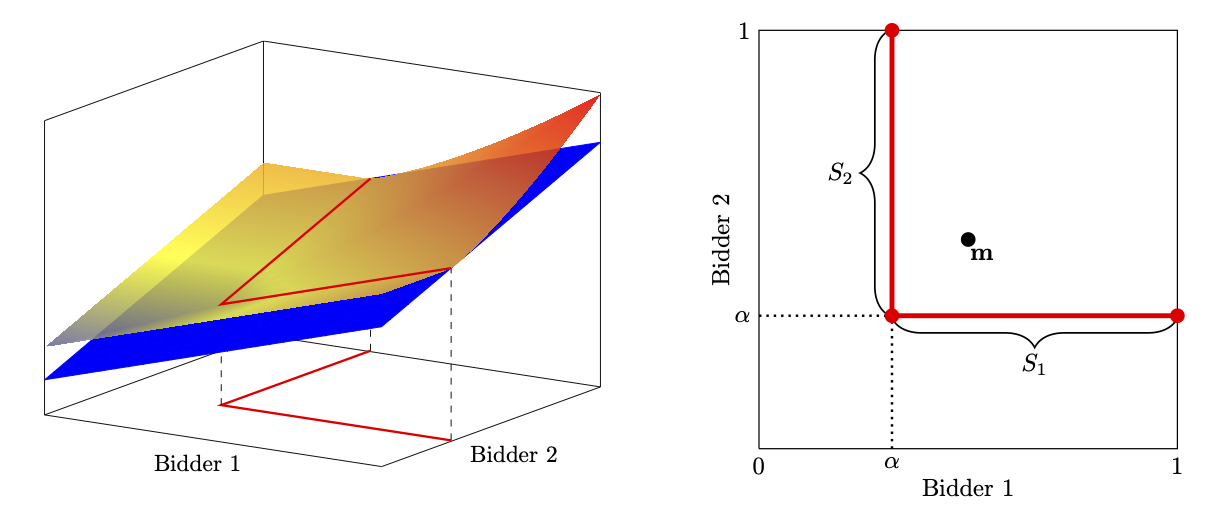
Figure 1: $\phi(\mathbf{v};G^{*})$ and the support of $F^{*}$ in the two bidder equilibrium ($m=\frac{1}{2})$.

Notes: On the left are the expected revenue function $\phi({\bf v};G^{*})$ (in red) induced by the seller’s equilibrium strategy $G^{*}$, the supporting affine function $L(\mathbf{v})$ (in blue), and the intersection of the two (in bold red). On the right, the support of $F^{*}$ (in bold red) and the mean point. When $m=\frac{1}{2}$, $\alpha\approx 0.317$.

To find an equilibrium with random reserve price, we first conjecture both nature’s and the seller’s strategies, and verify that they constitute a saddle point. We conjecture that nature’s strategy $F^{*}$ randomly picks one bidder to be the highest bidder, with value randomly drawn from CDF $H$, and sets the value of the second highest bidder to be as low as possible, perhaps to some lower bound $\alpha$ (which is yet to be determined), producing value profiles of the form $(v,\alpha)$ or $(\alpha,v)$, where $v$ is drawn from $H(v)$. Visually, the support of $F$ has an “L”-shape, as can be seen in the right panel of Figure 1. Formally, $\text{supp}(F^{*})=S_{1}\cup S_{2}$ where $S_{1}:=\left\{(v,\alpha):v\in(\alpha,1]\right\}$ and $S_{2}:=\left\{(\alpha,v):v\in(\alpha,1]\right\}$. Each segment $S_{i}$ contains the realized value profiles when the $i$th bidder is chosen to be the highest (and the other the second highest).

In order to pin down $H(v)$, we consider $H(v)$ which makes the seller indifferent across all (possible) reserve prices in $[0,1)$. Suppose the seller charges a reserve price $p$ facing bidders whose valuations are distributed as conjectured above. Then, he earns the revenue:

$$\eta(p;F) =\int_{V}\max\{v^{(2)},p\}\cdot 1_{\{v^{(1)}>p\}}dF$$

$$=\begin{cases}2\cdot\frac{1}{2}p(1-H(p))&\text{if }p>\alpha\\ \alpha&\text{if }p\leq\alpha\end{cases}$$

$$=\begin{cases}p(1-H(p))&\text{if }p>\alpha\\ \alpha&\text{if }p\leq\alpha.\end{cases}$$

For the seller to be indifferent across reserve prices, we require that for all $p\in(\alpha,1)$:

$$p(1-H(p))=\alpha,\text{ or }H(p)=\frac{p-\alpha}{p}.$$

Since $\lim_{p\to 1}H(p)=1-\alpha$, there must be a mass of $\alpha$ at $1$. Intuitively, for the seller to earn $\alpha$ even for $p$ arbitrarily close to 1, nature must put a mass of $\alpha$ at $1$. Our conjecture for $H$ is therefore:

$$H(v)=\begin{cases}0&\text{if }v\leq\alpha\\ \frac{v-\alpha}{v}&\text{if }v\in(\alpha,1)\\ 1&\text{if }v=1.\end{cases}$$

This distribution has density $h(v)=\frac{\alpha}{v^{2}}$ on $v\in(\alpha,1)$.

We can pin down $\alpha$ using the mean constraint on $F$. Each bidder $i$ is chosen to be the highest bidder with probability $1/2$ , in which case his valuation is determined by $H$. With the remaining probability, he is chosen to be the second highest bidder, with valuation $\alpha$. Hence, the mean of each bidder’s marginal distribution is:

$$m=\frac{1}{2}\alpha+\frac{1}{2}\left(\alpha+\int_{\alpha}^{1}vh(v)dv\right)=\alpha+\frac{1}{2}\int_{\alpha}^{1}\frac{\alpha}{v}dv=\alpha\left(1-\frac{1}{2}\ln(\alpha)\right),$$

This equation pins down a unique solution for $\alpha$, as we will later argue in the general $n$ bidder setting. When $m=1/2$, $\alpha=0.317$, as is depicted in Figure 1.

Next, we construct $G^{*}$ so that the conjectured $F^{*}$ will be a best response by nature. If we take a step back, we can see that for any given strategy $G$ by the seller, nature faces the following problem:

$$\inf_{F} \int_{V}\phi(\mathbf{v};G)dF$$ (3)

s.t. $$\int_{V}v_{i}(\mathbf{v})dF=m,\quad i=1,2$$

$$\int_{V}dF=1$$

$$F\geq 0,$$

where $v_{i}:V\to\mathbb{R}$ is the projection map on the $i$th bidder’s valuation and $\phi$ is the expected revenue from nature’s point of view, $\phi(\mathbf{v};G):=\int_{0}^{1}\max\{v^{(2)},p\}\cdot 1_{\{v^{(1)}>p\}}dG.$

It is useful to observe that this is a linear program in $F$. Given our conjecture for $F^{*}$, we can use the dual of this program to verify the optimality of $F^{*}$ with respect to the expected revenue function $\phi$ induced by the seller’s strategy $G$. We use a complementary slackness condition expressed in the following lemma. Note also that this lemma applies generally to the $n$-bidder case, and in fact, we will reuse this lemma to prove the optimality of our candidate $F^{*}$ in the general case.

Lemma 1.

Given the seller’s strategy $G$, $F^{*}$ is an optimal solution for nature’s problem if and only if $F^{*}$ is feasible and there exists an affine function $L:V\to\mathbb{R}$ such that

$$L(\mathbf{v}) \leq\phi(\mathbf{v};G),\text{ }\forall\mathbf{v}\in V\text{ and }$$

$$\text{\emph{supp}}(F^{*}) \subseteq\{\mathbf{v}:L(\mathbf{v})=\phi(\mathbf{v};G)\}.$$

Proof.

We prove the “if” part. The proof of the “only if” part, which requires the dual program, is relegated to the Appendix.

Suppose there exist feasible $F^{*}$ and an affine function $L$ satisfying the requirements. For any $F\in\mathcal{P}(V,m)$, this implies

$$\int_{V}\phi(\mathbf{v};G)dF^{*}=\int_{V}L(\mathbf{v})dF^{*}=\int_{V}L(\mathbf{v})dF\leq\int_{V}\phi(\mathbf{v};G)dF.$$

The first equality follows because $\phi$ and $L$ coincide on the support of $F^{*}$. The second equality follows because $L$ is affine and $F$ and $F^{*}$ have the same mean. The final inequality follows since $L(\mathbf{v})\leq\phi(\mathbf{v};G)$ for all $\mathbf{v}$. Hence $F^{*}$ is an optimal solution for nature. ∎

This lemma states that in order for our conjectured $F^{*}$ to be a best response to the seller’s strategy $G$, there must exist an affine function $L(\mathbf{v})$ such that expected revenue function $\phi$ induced by $G$ coincides with $L$ on the support of $F^{*}$, and is everywhere above $L$. The key implication of this lemma is that if we can find a strategy $G^{*}$ and an affine function $L$ such that the conditions of the lemma are satisfied, then $(G^{*},F^{*})$ is an equilibrium. We use these conditions as a tool for verifying an equilibrium. In particular, we will find $G$ that satisfies the conditions, given the $F^{*}$ we already conjectured.

Given the symmetry of $F^{*}$, it is without loss to focus on $S_{1}$ for evaluating $\phi({\bf v};G)$, where $S_{1}$ is the subset of the “L”-shape support in which nature picks the bidder 1 to be the highest bidder. On $S_{1}$, the expected revenue function will be:

$$\phi(\mathbf{v};G) =\int_{0}^{1}\max\{v^{(2)},p\}\cdot 1_{\{v^{(1)}>p\}}dG$$

$$=\int_{0}^{v_{2}}v_{2}g(p)dp+\int_{v_{2}}^{v_{1}}pg(p)dp,$$

assuming that $G$ admits density $g(p)$, which will be the case as we show below. For the conjectured $F^{*}$ to be optimal, Lemma 1 requires that $\phi(\mathbf{v};G)$ must be equal to some affine function $L(\mathbf{v})=c_{1}v_{1}+c_{2}v_{2}+d$ on this segment. This implies that for all $(v,\alpha)\in S_{1}$:

$$\frac{\partial\phi}{\partial v_{1}}(v,\alpha)=vg(v)=c_{1},\text{ or }g(v)=\frac{c_{1}}{v}.$$

This logic applies symmetrically if nature had picked bidder 2 to be the highest bidder instead, so we can consider $c_{1}=c_{2}=c$. This pins down the form of the sender’s strategy for $p\in[\alpha,1]$. In order to satisfy the remaining conditions of the Lemma, we now can find $c$ so that $\phi\geq L$ for all value profiles.

Next, consider any ${\bf v}=(v,\alpha)$, for $v>\alpha$. Since $(v,\alpha+\epsilon)$ is outside $\text{supp}(F^{*})$, for any $\epsilon>0$ or $\epsilon<0$, Lemma 1 requires that $\phi(v,\alpha+\epsilon)\geq L(v,\alpha+\epsilon)$, for any $\epsilon>0$ or $\epsilon<0$ and that $\phi(v,\alpha)=L(v,\alpha)$. This implies that:

$$\frac{\partial\phi}{\partial v_{2}}(v,\alpha)=\frac{\partial L}{\partial v_{2}}(v,\alpha)\implies G(\alpha)=c.$$

Since $G$ must integrate to $1$, we find:

$$1=\int_{0}^{1}dG(p)=G(\alpha)+\int_{\alpha}^{1}\frac{G(\alpha)}{p}dp=G(\alpha)(1-\ln(\alpha)),$$

so:

$$c=G(\alpha)=\frac{1}{1-\ln(\alpha)}.$$

We will choose $G(0)=G(\alpha)=c$, so that the seller places the entire mass of $c$ at $p=0$. This will be seen to be optimal for the seller, although it is possible that there could be other payoff-equivalent equilibria in which the seller may put density on $[0,\alpha]$. Note that unlike the equilibrium for single buyer case in Carrasco et al. (2018), the support of the seller and nature do not fully coincide. In other words, with positive probability, the seller chooses a reserve price that guarantees sale. As we will see later, this probability increases as the number of bidders increases. The intuition is that as competition increases, the seller can rely less on a “binding” reserve price to guarantee revenue as competition between the bidders limits the ability of nature to suppress revenue.

Finally, the condition $\phi=L$ at $(\alpha,\alpha)$ pins down the constant $d=\frac{\alpha}{1-\ln(\alpha)}$ of $L({\bf v})$. Thus, the strategy $G^{*}$ and the affine function $L$ are fully characterized as follows:

$$G^{*}(p) =\begin{cases}\int_{\alpha}^{p}\frac{1}{r\left(1-\ln(\alpha)\right)}dr+\frac{1}{1-\ln(\alpha)}&\text{if }p>\alpha\\ \frac{1}{1-\ln(\alpha)}&\text{if }p\leq\alpha\end{cases}$$

$$L(\mathbf{v}) =\frac{1}{1-\ln(\alpha)}(v_{1}+v_{2})-\frac{\alpha}{1-\ln(\alpha)}.$$

One can check that $\phi({\bf v};G^{*})\geq L(\mathbf{v})$ for all $\mathbf{v}\in V$ and $\phi=L$ on the support of $F^{*}$, satisfying the conditions of Lemma 1. The left panel of Figure 1 visualizes how $\phi$ and $L$ satisfy this requirement for the case of $m=1/2$. Lemma 1 guarantees that $F^{*}$ will be a best response to $G^{*}$. Recall that $F^{*}$ was constructed to make the seller indifferent across all reserve prices $p\in[\alpha,1)$ and thus $G^{*}$ is a best response to $F^{*}$. Thus, we have found an equilibrium for the two-bidder game with symmetric mean constraints.

Two differences emerge with the introduction of the second bidder (compared to the monopoly pricing equilibrium in Carrasco et al. (2018)). First, as mentioned earlier, the seller puts mass strictly below the support of the marginal distribution of $F$. Second, the marginal distribution of $F$ has two mass points, one at the upper bound $v=1$ (as in the single buyer equilibrium), and one at the lower bound $\alpha$ (unlike the single buyer equilibrium).

3.3 Optimal reserve price with $n$ (possibly asymmetric) bidders

In this section, we present a profile of candidate strategies $(G^{*},F^{*})$ that form a second-price auction equilibrium in the $n$-bidder case with (possibly) asymmetric mean constraints. The equilibrium is a natural extension of the two bidder, symmetric mean equilibrium. In Appendix A.3, we will prove that these strategies satisfy the saddle point inequalities.

Nature’s strategy.

Nature’s worst case distribution retains the “L”-shape structure, randomly choosing a bidder to be the highest bidder (with value distributed according to $H(v)$) while setting the valuations of the remaining bidders to a lower bound $\alpha$. However, a few modifications are introduced when there are bidders with asymmetric means. First, the “L”-shape joint distribution may not include all $n$ bidders. If there are bidders with means strictly less than $\alpha$, they cannot be included in this distribution without violating these constraints. Instead, nature will set the marginal distributions of these bidders to a point mass on their means. Second, among the “active” bidders who are included in the distribution, nature selects one of them to be the highest-value bidder with non-uniform probabilities. We will see that higher mean bidders are more likely to be selected as the highest-value bidder.

We will proceed to describe the set of active bidders and the joint distribution among the active and inactive bidders.

Selection of Active Bidders.

Recall that the bidders are indexed such that $m_{1}\geq m_{2}\geq...\geq m_{n}$. Suppose in the chosen distribution, there exists a cutoff $k$ such that bidders $i=1,...,k$, with mean $m_{i}\geq m_{k}$ are included in the $L$-shape distribution (the “active” bidders) and the remaining bidders $k+1,...,n$ are excluded (the “inactive” bidders). Following the reasoning provided in Section 3.2, we postulate that the lower bound of the support is $\alpha_{k}(\bar{m}_{k})$, where $\bar{m}_{k}=\frac{1}{k}\sum_{i=1}^{k}m_{i}$ is the average of the highest $k$ mean constraints (i.e. the mean of the mean constraints among the active bidders) and $\alpha_{k}(x)$ is the solution of $x=\alpha\left(1-\frac{1}{k}\ln(\alpha)\right)$. For this to be a consistent with the hypothesis, it must be the case that $m_{i}>\alpha_{k}(\bar{m}_{k})$ for all $i\leq k$ and $m_{r}\leq\alpha_{k}(\bar{m}_{k})$ for all $r>k$. This reasoning suggests the cutoff $k$ is determined by

$$k\equiv\min \left\{\ell:m_{i}>\alpha_{\ell}(\bar{m}_{\ell})\text{ for }i\leq\ell,m_{r}\leq\alpha_{\ell}(\bar{m}_{\ell})\text{ for }r>\ell\right\},$$ (4)

For example, if there are $n=3$ bidders with $m_{1}=0.6$, $m_{2}=0.5$, and $m_{3}=0.1$, the cutoff $k$ will be $2$ since $\bar{m}_{2}=\frac{m_{1}+m_{2}}{2}=0.55$, $\alpha_{2}(\bar{m}_{2})\approx 0.366$, and $m_{1},m_{2}>\alpha_{2}(\bar{m}_{2})$ with $m_{3}<\alpha_{2}(\bar{m}_{2})$. There will be two active bidders, since the mean of the third bidder’s valuation is too low. Note that if the means of all $n$ bidders are symmetric $m_{1}=...=m_{n}$, then the cutoff is $k=n$ and all bidders are active.

We find that given any $n$ bidders with means $\{m_{i}\}_{i=1}^{n},$ we can always find such a cutoff through a simple iterative procedure.

Lemma 2.

The cutoff $k$ in (4) always exists.

Proof.

See Appendix A.2. ∎

Note in addition that $\alpha_{k}(x)$ is well-defined for any $k\in[n]$ and $x\in[0,1]$. To see this, note that when $\alpha=0$, $\alpha\left(1-\frac{1}{k}\ln(\alpha)\right)=0$ and when $\alpha=1$, this is equal to $1$. Since the expression is continuous and strictly increasing, there exists a unique $\alpha$ such that this equation holds. Explicitly, $\alpha_{k}(\bar{m}_{k})$ is:

$$\alpha_{k}(\bar{m}_{k})=\exp\left(k+W_{-1}\left(-\frac{k\bar{m}_{k}}{e^{k}}\right)\right),$$

where $W_{-1}$ is the lower branch of the Lambert $W$ function. When all $n$ bidders have means equal to $m$, the equation for $\alpha$ becomes

$$m=\alpha\left(1-\frac{1}{n}\ln(\alpha)\right).$$ (5)

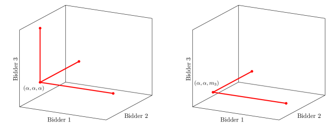
Figure 2: Support of $F^{*}$ with symmetric and asymmetric mean constraints

Notes: On the left panel is an example of $F^{*}$ with $n=3$ bidders with symmetric mean constraints. On the right panel is an example of $F^{*}$ with $n=3$ bidders but only $k=2$ active bidders, in which $m_{3}<\alpha_{2}(\bar{m}_{2})$.

Worst-case Distribution.

With the cutoff $k$ from (4) in hand, we can now construct nature’s worst-case distribution $F^{*}$. In $F^{*}$, each inactive bidder $j\in\{k+1,...,n\}$ draws value $m_{j}$ with probability one. Each active bidder $i\in\{1,...,k\}$ is selected to be the highest bidder with probability $\theta_{i}$, in which case all other active bidders draw valuations $\alpha$ and the highest bidder’s value is distributed according to a CDF $H(v)$. A typical value profile will be as follows:

$${\bf v}_{i}(v)\equiv(\underbrace{\alpha,\alpha,...,v,...,\alpha}_{k\text{ active bidders}},\underbrace{m_{k+1},m_{k+2},...,m_{n}}_{n-k\text{ inactive bidders}}),$$ (6)

where bidder $i$ has the highest value of $v\sim H(v)$.

As in the two-bidder case, the highest bidder’s valuation is distributed according to the CDF

$$H(v)=\begin{cases}0&\text{if }v\leq\alpha\\ \frac{v-\alpha}{v}&\text{if }v\in(\alpha,1),\\ 1&\text{if }v=1.\end{cases}$$

As with the two bidder case, $H(v)$ ensures that the seller is indifferent with his choice of reserve price within the support of $H$.

The probabilities $\theta_{i}$ that an active bidder $i$ is selected as the highest-value bidder are chosen to satisfy the mean constraints

$$(1-\theta_{i})\alpha+\theta_{i}\left(\alpha+\int_{\alpha}^{1}vh(v)dv\right)=m_{i}.$$ (7)

Solving for $\theta_{i}$, we obtain

$$\theta_{i}=\frac{m_{i}-\alpha}{\alpha\ln(\frac{1}{\alpha})}.$$

Naturally, the higher the mean $m_{i}$, the higher the selection probability $\theta_{i}$. In other words, $\theta_{1}\geq\theta_{2}\geq...\geq\theta_{k}$. Nature adjusts the selection probabilities to “soak up” all the asymmetries, while ensuring that the value distribution of the highest bidder is the same (given by $H$) regardless of which bidder is chosen. In an important sense, Nature eliminates asymmetries from the perspective of the seller, which ultimately eliminates the need for the seller to treat bidders differently.

Finally, summing across equations (7) for across all $k$ active bidders, we obtain the following condition for the lower bound $\alpha$,

$$\frac{1}{k}\sum_{i=1}^{k}m_{i}=\bar{m}_{k} =\alpha\left(1-\frac{1}{k}\ln(\alpha)\right),$$

which confirms that the lower bound $\alpha$ is indeed equal to $\alpha_{k}(\bar{m}_{k})$.

Altogether, nature’s strategy $F^{*}$ is:

$$F^{*}(U)\equiv \sum_{i=1}^{k}\theta_{i}\cdot H(\text{Proj}_{i}(U))$$ (8)

for any measurable subset $U$ of $\text{supp}(F^{*})=\bigcup_{i\in[k]}\{{\bf v}_{i}(v):v\in(\alpha,1]\}$, where ${\bf v}_{i}(v)$ are the value profiles defined in (6), $\text{Proj}_{i}:U\to\mathbb{R}$ is the projection map on to the $i$th bidder’s valuation, and (overloading notation) $H$ is the measure induced by the CDF $H$.

Seller’s Strategy.

The seller’s strategy is to randomize his reserve price according to the CDF:

$$G^{*}(p)=\begin{cases}\int_{\alpha}^{p}\frac{1}{r\left(k-1-\ln(\alpha)\right)}dr+\frac{k-1}{k-1-\ln(\alpha)}&\text{if }p>\alpha\\ \frac{k-1}{k-1-\ln(\alpha)}&\text{if }p\leq\alpha.\end{cases}$$ (9)

In other words, the seller chooses $p\in[\alpha,1]$ with density $g(p)=\frac{1}{p\left(k-1-\ln(\alpha)\right)}$ and places a point mass of $\frac{k-1}{k-1-\ln(\alpha)}$ on the reserve price $p=0$. As in the two-bidder case, the density is constructed to prevent nature from deviating from $F^{*}$ by satisfying the conditions of Lemma 1.

Note that from the seller’s perspective, the particular asymmetries between bidders do not matter; the optimal reserve price only depends on the number of active bidders $k$ and the lower bound $\alpha$. This is because all the payoff-relevant features remain the same regardless of which bidder is picked as the winner: the highest bidder’s value is always drawn from $H(v)$ and the second-highest value is always $\alpha$. Hence, the seller’s optimal reserve price is symmetric across bidders.

The pair of strategies $(G^{*},F^{*})$ satisfy the saddle point condition, proving that $S_{G^{*}}$ is revenue guarantee optimal among all second-price auction mechanisms.

Theorem 1.

The strategy profile $(G^{*},F^{*})$ satisfies the saddle point condition in (2) and therefore are an equilibrium of the zero sum game. The revenue guarantee is $\Psi(G^{*},F^{*})=\alpha_{k}(\bar{m}_{k})$.

Proof.

See Appendix A.3. ∎

We explore several implications of this theorem. First, suppose there are $n$ bidders with symmetric means $\{m_{i}\}_{i=1}^{n}=m$. Let $G_{n}^{*}$ and $F_{n}^{*}$ be the equilibrium strategy in this auction.

Corollary 1.

Given a sequence of auctions with symmetric mean bidders $\{m_{i}\}_{i=1}^{n}=m$, there exists a sequence of equilibria $\left(G_{n}^{*},F_{n}^{*}\right)$ such that the random reserve price $p_{n}\sim G_{n}^{*}$ converges to zero in probability as $n\to\infty$. Furthermore, the optimal revenue guarantee $\Psi(G_{n}^{*},F_{n}^{*})=\alpha_{n}$ increases in $n$ and converges to $m$ at rate $O(1/n)$. The rent obtained by the highest value bidder is $\alpha_{n}\log(1/\alpha_{n})$, which converges to $m\log(1/m)\leq 1/e$.

Proof.

We define $\alpha_{n}$ to be the solution of $m=\alpha\left(1-\frac{1}{n}\ln(\alpha)\right)$ when there are $n$ bidders and symmetric means equal to $m$. First, we observe that $\alpha_{n}$ is increasing in $n$. This is because the RHS of (5) is decreasing in $n$, for any $\alpha\in(0,1)$. Hence, as $n$ increases, the RHS shifts down. Since RHS is an increasing function of $\alpha$, the $\alpha$ satisfying (5) must increase as $n$ increases. Furthermore, as $n$ goes to infinity the RHS converges to $\alpha$, which implies that $\alpha_{n}$ converges to $m$.

The convergence of the reserve price results from observing that the reserve price $p_{n}\sim G_{n}^{*}$ with $G_{n}^{*}$ defined in (9) converges in probability to zero as $n\to\infty$, as for any $\epsilon>0$

$$\mathbb{P}(p_{n}>\epsilon)=1-G_{n}^{*}\left(\epsilon\right)\leq 1-G_{n}^{*}\left(\alpha_{n}\right)=\frac{-\ln(\alpha_{n})}{n-1-\ln(\alpha_{n})}\rightarrow 0.$$

We can see that that since $\alpha_{n}$ solves $m=\alpha_{n}\left(1-\frac{1}{n}\ln(\alpha_{n})\right)$ we have that $m-\alpha_{n}=\frac{\alpha_{n}\ln\left(\frac{1}{\alpha_{n}}\right)}{n}\leq\frac{1}{ne}$, so the rate of convergence is $O(\frac{1}{n})$.

Finally, the mean of the distribution of the highest-value bidder $H(v)$ can be computed as $\alpha(1+\log(1/\alpha))$. The highest bidder pays $\alpha$ and is thus left with $\alpha\log(1/\alpha)$.

∎

Corollary 2.

Fix two situations with $n$ and $n^{\prime}>n$ bidder, where all bidders have the same mean $m$. The distribution of the highest bidder’s value $H_{n^{\prime}}$ first-order stochastically dominates $H_{n}$.

Proof.

The difference $H_{n}(v)-H_{n^{\prime}}(v)$ for all $v\in[0,1]$ is as follows:

$$H_{n}(v)-H_{n^{\prime}}(v)=\begin{cases}0&\text{if }v\leq\alpha_{n}\\ \frac{v-\alpha_{n}}{v}&\text{if }v\in(\alpha_{n},\alpha_{n^{\prime}}]\\ \frac{\alpha_{n^{\prime}}-\alpha_{n}}{v}&\text{if }v\in(\alpha_{n^{\prime}},1)\\ 0&\text{if }v=1.\end{cases}$$

As shown in the proof of Corollary 1, $\alpha_{n}$ is increasing in $n$. Hence, for all $v\in[0,1]$, $H_{n}(v)\geq H_{n^{\prime}}(v)$. ∎

Corollary 1 says that as the number of bidders grows large, the equilibrium revenue converges to the mean of a single bidder’s valuation, which implies that the seller extracts a single bidder’s surplus in the limit. Additionally, it states that there exists a sequence of equilibria such that the seller’s reserve price converges to zero in probability, as the number of bidders goes to infinity (Figure 3 shows the effect of increased competition from $n=2$ to $n=10$). The asymptotic behavior of the equilibrium reserve price strategy is consistent with the widespread observation that reserve prices tend to be lower than is prescribed by the standard (Bayesian) theory under the estimated distribution of value profiles, as noted by Haile and Tamer (2003) in timber auctions, Bajari and Hortacsu (2003) in eBay auctions, and McAfee et al. (2002) in real estate auctions.

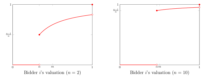
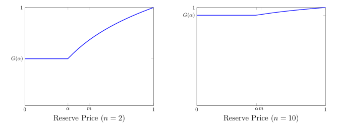
Figure 3: Strategies for nature and the seller when $n=2$ and $n=10$ ($m=\frac{1}{2}$).

Notes: These are the equilibrium strategies for nature and the seller when $n=2$ and $n=10$ and all bidders have symmetric means $m=1/2$. In red is the CDF of the marginal distribution of nature’s equilibrium strategy $F^{*}$. In blue is $G^{*}$, or the CDF of the seller’s strategy over reserve price. When $n=2$, $\alpha\approx 0.317$ and when $n=10$, $\alpha\approx 0.464$. Observe that as the number of bidders increases, the seller’s mass on $p=0$ increases towards 1, and $\alpha$ increases towards the mean $m$.

A key feature of this equilibrium is that the seller randomizes in reserve price. Since nature can only pick one worst-case distribution, randomization allows the seller to hedge against nature. Randomization protects the seller against states of the world that are adverse for a particular reserve price, and it forces nature to minimize revenue across multiple value realizations.

As the number of bidders increases however, the role of reserve price disappears, as the probability of binding reserve prices vanishes. In essence, competition between bidders appears substitutes for a reserve price. The intuition of this result is that competition constrains the seller’s worst case belief: as the number of bidders increases, nature is compelled to increase the value of the second-highest bidder $\alpha$ to maintain the mean constraint. Furthermore, the marginal distribution of each bidder converges to a point mass on $\alpha$ (as each bidder is the second-highest bidder with probability $\frac{n-1}{n}$). In the limit, the worst-case joint distribution becomes the point mass distribution on the value profile consisting of $\alpha$ for all bidders, which itself converges to $m$. The optimal strategy for the seller facing a point mass on ${\bf m}=(m,...,m)$ is to charge a reserve price of zero.

4 Optimal Competitive Mechanism

In this section, we explore the performance of the optimal second-price auction within a broad class of mechanisms and show that the second-price auction with an optimal reserve price is revenue-guarantee optimal within this class.

We begin with some definitions. Given a fixed value distribution $F$, we say that a realized bidder-type $(i,v_{i})$ is clearly low if (1) with probability $1$ there exists some bidder $j\neq i$ with a higher valuation than $v_{i}$ and (2) conditional on bidder $j$ having a higher valuation, bidder $i$’s distribution is a point mass on $v_{i}$. Formally, we define the set of clearly low bidder-values to be:

$$\xi(F)=\{(i,v):\exists j\neq i\text{ s.t. }\mathbb{P}_{F}(v_{j}>v|v_{i}=v)=1\text{ and }\mathbb{P}_{F}(v_{i}=v|v_{j}>v)=1\}.$$

The event has a clear implication for what bidders know when they have a common knowledge about the value distribution $F$. In that case, whenever a bidder realizes a clearly low value $v$, it becomes common knowledge between $i$ and some bidder $j$ (whose identity may be unknown to $i$) that bidder $j$ has a strictly higher value than $v$ and bidder $i$ has exactly $v$.

We say that a bidder-type never wins at $\Gamma(M,I,F)$ if he is assigned the good with probability zero in every Bayes-Nash equilibrium in undominated strategies of the game induced by $(M,I,F)$. The class of competitive mechanisms is defined as:

$$\widehat{\mathcal{M}}=\{M\in\mathcal{M}:\forall F\in\mathcal{P}(V),(i,v)\in\xi(F)\text{ never wins at }\Gamma(M,I_{0},F)\}.$$

This definition imposes a very mild restriction on the set of possible mechanisms. First, the definition rules out behavior of the mechanism only under the UCP information structure $I_{0}$. Second, it only restricts allocation in rather atypical realizations of the value distribution when two bidders both know that one has a higher value than the other with complete certainty (and the higher-value bidder must know the lower-value bidder’s value exactly). These realizations do not exist in many typical value distributions, e.g. if values are drawn iid from a non-degenerate distribution, and no restriction is imposed for such distributions.

Given the mildness of this restriction, the class of competitive mechanisms encompasses many standard auction mechanisms without reserve prices or with a common reserve price. This includes all efficient mechanisms (which allocate the good to the highest value bidder) but also includes some inefficient mechanisms, such as the first-price auction.

Lemma 3.

The second-price auction and the first-price auction, both possibly with a common (possibly random) reserve price, are competitive mechanisms.

Proof.

See Appendix A.4. ∎

Evidently, the class of competitive mechanisms is not the largest class of mechanisms for which the second-price auction is revenue-guarantee optimal. For example, lottery mechanisms (which give away the good to a random bidder) or an all-pay auction with reserve prices uniformly above or below $\alpha$ are not competitive mechanisms but are still revenue dominated by the optimal second-price auction given $F^{*}$. Rather, we focus on this particular class of mechanisms since it prescribes a natural and weak restriction on admissible mechanisms.

Our main result is that the optimal second-price auction found in section 3 obtains the optimal revenue guarantee within the class of competitive mechanisms.

Theorem 2.

The second-price auction mechanism $S_{G^{*}}$ with the optimal reserve price $G^{*}$ in (9) obtains the optimal revenue guarantee out of all competitive mechanisms. In other words, for any $M\in\widehat{\mathcal{M}}$ and $(F,I)\in\mathcal{P}(V,\{m_{i}\}_{i=1}^{n})\times\mathcal{I}$.

$$\mathcal{R}(M,I_{0},F^{*})\leq\mathcal{R}(S_{G^{*}},I_{0},F^{*})\leq\mathcal{R}(S_{G^{*}},I,F),$$

where $F^{*}$ is the worst-case distribution in (8) and $I_{0}$ is the UCP information structure. These inequalities imply:

$$S_{G^{*}}\in\arg\max_{M\in\hat{M}}\inf_{F,I}\mathcal{R}\left(F,I,M\right).$$

Proof.

See Appendix A.5. ∎

As mentioned before, although we restrict ourselves to the set of competitive mechanisms, this by no means captures all of the mechanisms within which $S_{G^{*}}$ revenue dominates, given $(F^{*},I_{0})$. In fact, we can observe from the proof that $S_{G^{*}}$ revenue-guarantee dominates any mechanism for which $\mathcal{R}(M,I_{0},F^{*})\leq\alpha$.

At the same time, it is not true that $S_{G}$ is optimal in the fully unrestricted class of mechanisms. When facing $(F^{*},I_{0})$, the seller can do strictly better with a mechanism that is not competitive.

Example 1.

Consider a setting with two bidders with identical means $m\in(0,1)$, with valuations distributed by $F^{*}$.

Consider the following mechanism. Both bidders are asked to report who the clearly low bidder is (the bidder who draws $\alpha$) and a bidder who reports himself not to be reports his value. If there is no consensus on the clearly low bidder, then neither bidder gets the good and there is no payment. If bidder $i$ is a consensus low bidder, then bidder $j\neq i$ gets the good if and only if his value is strictly above $1-\epsilon$ at price $1-\epsilon$. Otherwise, the low bidder gets the good at price $\alpha-\epsilon$. For $\epsilon>0$ sufficiently small, it is a weak dominant strategy for the low bidder to report truthfully. Further, it is a best response for the high bidder to report truthfully about the other bidder being clearly low and about true value. Indeed, the strategy is undominated.

Hence, the expected revenue from the equilibrium is:

$$\sum_{i=1}^{2}\mathbb{E}_{F^{*}}[t_{i}({\bf v})] =\frac{1}{2}\sum_{i=1}^{2}\left[(1-H(1-\epsilon))(1-\epsilon)+H(1-\epsilon)(\alpha-\epsilon)\right]$$

$$\geq\alpha(1-\epsilon)+\frac{1-\epsilon-\alpha}{1-\epsilon}(\alpha-\epsilon).$$

As $\epsilon\to 0$, the RHS converges to $\alpha+(1-\alpha)\alpha>\alpha$ so for $\epsilon$ small enough the revenue exceeds $\alpha$.

We can make a few remarks about the mechanism. First, the above mechanism is implausible as it involves extreme discrimination and is very sensitive to the particular structure of the value distribution. It is never robustly optimal itself. Nature could simply choose the two point distribution placing mass at $\alpha-2\epsilon$ and some $z\in(m,1-\epsilon)$, which would admit an equilibrium in which no sale arises. The second-price auction does not suffer from such instabilities and does not discriminate between bidders even if the seller has ex-ante knowledge of asymmetries between the bidders.

Second, the above mechanism is also susceptible to collusion by bidders. Facing the mechanism, the bidders would find it optimal to coordinate their reports so that the high bidder is the low bidder and the low bidder reports less than $1-\epsilon$ for his value, so that the high value bidder always gets the good at price $\alpha-\epsilon$. The bidder surplus would be sufficiently high so that such a side contract can be mutually beneficial (and incentive compatible since they know who the low bidder is as common knowledge). By contrast, the second price auction does not leave any room for collusion, since the allocation is efficient among the bidders, conditional on it being allocated to somebody.

5 Conclusion

We have studied the seller’s optimal selling mechanism to multiple potential buyers, subject to moment conditions of the distribution of bidders’ values. We have identified the worst-case distribution chosen by nature and the optimal reserve price strategy of the seller as the equilibrium of a zero-sum, simultaneous move game. We have found that among a wide class of Bayesian mechanisms, a second-price auction with a random, symmetric reserve price obtains the optimal revenue guarantee even in the presence of a priori asymmetric means for the bidders. In addition, we have shown that when bidders have identical means and as the number of bidders increases, the optimal second-price auction involves a non-binding reserve price and the revenue guarantee converges to the best possible revenue guarantee at rate $O(1/n)$.

Appendix A Proofs

A.1 Proof of “Only if” of Lemma 1

Proof.

To prove the converse of Lemma 1, we construct the dual of nature’s minimization problem in (3):

$$\max_{\gamma_{i},\eta} \sum_{i=1}^{n}\gamma_{i}\cdot m+\eta$$

s.t. $$\sum_{i=1}^{n}\gamma_{i}v_{i}(\mathbf{v})+\eta\leq\phi(\mathbf{v};G),\text{ }\forall\mathbf{v}\in V.$$

The dual variables $\gamma_{i}$ and $\eta$ together belong in $\mathbb{R}^{n+1}$. This representation follows the dual of the semi-infinite linear program in Anderson and Nash (1987).

The primal is bounded above by $1$, and the measure $F=\delta_{\mathbf{m}}$, which assigns all mass to the mean point $\mathbf{m}=(m,m,...,m)$, is in the interior of the primal cone. By Theorem 3.12 in Anderson and Nash (1987), strong duality holds.

The dual solution $(\gamma^{*},\eta^{*})$ defines an affine function $L(\mathbf{v})=\left\langle\gamma^{*},\mathbf{v}\right\rangle+\eta^{*}$. Given the primal solution, we can rewrite the dual in terms of this affine function.

$$\max_{L} \int_{V}L(\mathbf{v})dF$$

s.t. $$L(\mathbf{v})\leq\phi(\mathbf{v};G),\text{ }\forall\mathbf{v}\in V.$$

The constraint of the dual guarantees that the affine function is below the expected revenue function. There is no duality gap, which means:

$$\int_{V}L(\mathbf{v})dF^{*}=\int_{V}\phi(\mathbf{v};G)dF^{*}.$$

Therefore, points at which $L(\mathbf{v})<\phi(\mathbf{v};G)$ must only occur on a measure zero set with respect to $F^{*}$. By the definition of the support, we obtain:

$$\forall\mathbf{v}\in\text{supp}(F^{*}),\text{ }L(\mathbf{v})=\phi(\mathbf{v};G).$$

∎

A.2 Proof of Lemma 2

Proof.

We can use a straightforward algorithm to find $k$.

First, we begin with $i:=2$, the bidder with the second-highest mean constraint. We calculate $\bar{m}_{i-1}$ and $\alpha_{i-1}(\bar{m}_{i-1})$ and check whether $m_{i}\leq\alpha_{i-1}(\bar{m}_{i-1})$. If so, then we set $k=i-1$. If not, then we increment the index $i:=i+1$ and repeat the same procedure. If $i$ reaches $n+1$, then $k=n$.

There are finitely many bidders so this algorithm will terminate. Since $k$ is returned by the algorithm only if $m_{k+1}\leq\alpha_{k}(\bar{m}_{k})$ (or if $k$ is the last bidder), for all bidders with index $p$ greater than $k$, $m_{p}\leq m_{k+1}\leq\alpha_{k}(\bar{m}_{k})$.

It remains to show that $m_{j}>\alpha_{k}(\bar{m}_{k})$ for all $j\leq k$. It must be true that $m_{k}>\alpha_{k-1}(\bar{m}_{k-1})$, otherwise $k-1$ would have been the outputted cutoff. It suffices to show that $m_{k}>\alpha_{k}(\bar{m}_{k})$. Suppose to the contrary that:

$$\alpha_{k-1}(\bar{m}_{k-1})<m_{k}\leq\alpha_{k}(\bar{m}_{k}).$$

The RHS of the equation $x=\alpha\left(1-\frac{1}{\ell}\ln(\alpha)\right)$ is increasing in $\alpha$, which means that for the equation satisfied by $\alpha_{k-1}(\bar{m}_{k-1})$ (shortening notation to $\alpha_{k-1}$):

$$\bar{m}_{k-1}=\alpha_{k-1}\left(1-\frac{1}{k-1}\ln(\alpha_{k-1})\right)<m_{k}\left(1-\frac{1}{k-1}\ln(m_{k})\right),$$ (10)

and likewise

$$\bar{m}_{k}=\alpha_{k}\left(1-\frac{1}{k}\ln(\alpha_{k})\right)\geq m_{k}\left(1-\frac{1}{k}\ln(m_{k})\right).$$ (11)

We can multiply (10) by $k-1$ and (11) by $k$ and subtract the former from the latter to obtain:

$$k\bar{m}_{k}- (k-1)\bar{m}_{k-1}>m_{k}$$

$$m_{k}>m_{k},$$

which is a contradiction. Hence for all $j\leq k$, $m_{j}\geq m_{k}\geq\alpha_{k}(\bar{m}_{k})$.

The $k$ returned by the algorithm satisfies both conditions required for the cutoff and furthermore, it will be the minimum index that does so since we iterate from the smallest index $1$. ∎

A.3 Appendix: Proof of Theorem 1

To prove Theorem 1, we will first show in Section A.3.1 that the seller’s strategy $G^{*}$ is optimal given $F^{*}$. In Section A.3.2, we will prove that nature’s strategy $F^{*}$ is optimal given $G^{*}$.

A.3.1 Seller’s problem

First, we show that for the $F^{*}$ described above, $G^{*}$ is a best response by the seller. In other words, we will show the following inequality holds for all $G\in\mathcal{P}\left([0,1]\right)$:

$$\Psi(G,F^{*})\leq\Psi(G^{*},F^{*}).$$

Proof.

Recall that $F^{*}$ has the following form:

$$F^{*}(U)=\sum_{i=1}^{k}\theta_{i}\mathbf{1}_{S_{i}}\cdot H(\textrm{Proj}_{i}(U)),$$

where $k$ is the cutoff index from Lemma 2, which determines the number of active bidders. The distribution of the highest bidder’s value $H(v)$ is:

$$H(v)=\begin{cases}0&\text{if }v\leq\alpha\\ \frac{v-\alpha}{v}&\text{if }v\in(\alpha,1)\\ 1&\text{if }v=1.\end{cases}$$

Using the same notation as in the two bidder case, we let $\eta(p;F)$ denote the seller’s expected revenue under reserve price $p$ given nature’s strategy $F.$

$$\eta(p;F):=\int_{V}\max\{v^{(2)},p\}\cdot 1_{\{v^{(1)}>p\}}dF.$$

Similar to the two bidder example, we will proceed to show that our candidate $F^{*}$ makes the seller indifferent across all reserve prices (at least in $[0,1)$). Under $F^{*}$, if the seller sets the reserve price below $\alpha$, a sale will always occur and the seller will receive the second highest value, $\alpha$. If the seller sets the reserve price above $\alpha$, then he will make a sale with probability $H(p)$ and receive the reserve price $p$ as revenue. Hence, the seller’s payoff under $F^{*}$ from a given reserve price is:

$$\eta(p;F^{*}) =\begin{cases}\sum_{i=1}^{k}\theta_{i}\cdot p(1-H(p))&\text{if }p>\alpha\\ \alpha&\text{if }p\leq\alpha\end{cases}$$

$$=\begin{cases}p(1-H(p))&\text{if }p>\alpha\\ \alpha&\text{if }p\leq\alpha.\end{cases}$$

Note that the $n-k$ inactive bidders do not affect the seller’s expected revenue, as the second-highest value $\alpha$ is always greater than their valuations. Note also that the number of bidders and their selection probabilities $\theta_{i}$ only affect the seller through their impact on $\alpha$. With the exception of $\alpha$, the expected revenue to the seller $\eta$ for any reserve price $p$ is exactly the same as in the two-bidder, symmetric mean example.

For any reserve price $p\in[0,1)$, the revenue to the seller will be:

$$p(1-H(p))=p\left(1-\frac{p-\alpha}{p}\right)=\alpha.$$

When $p=1$, the revenue may be smaller, depending on the tie breaking rule. Observe however that $G^{*}$ does not put any mass at 1, so

$$\Psi(G^{*},F^{*})=\alpha\geq\Psi(G,F^{*}),$$

for any $G\in\mathcal{P}\left([0,1]\right)$. Hence, $G^{*}$ in Theorem 1 is a best response. ∎

A.3.2 Nature’s problem

Now we will prove that for the $G^{*}$ in Theorem 1, $F^{*}$ is a best response by nature. We will show that for any $F\in\mathcal{P}(V,m)$,

$$\Psi(G^{*},F^{*})\leq\Psi(G^{*},F).$$

Equivalence with a $k$-bidder auction.

Since the $n-k$ inactive bidders do not affect the revenue, we can prove the saddle point inequality using the $F^{*}$ distribution containing only the $k$ active bidders, which simplifies the problem. Consider a new auction $(V_{k},\{m_{i}\}_{i=1}^{k})$, in which we include only the $k$ active bidders in the “L”-shape joint distribution of $F^{*}$.

For any distribution of value profiles in the original $n$-bidder auction $F\in\mathcal{P}(V,\{m_{i}\}_{i=1}^{n})$, we can project this distribution on the $k$ active bidders and obtain $F_{k}\in\mathcal{P}(V_{k},\{m_{i}\}_{i=1}^{k})$. This distribution is exactly identical to $F$ for the $k$ active bidders, but no longer includes the $n-k$ inactive bidders.

We see that from nature’s point of view, removing these bidders is without loss.

Lemma 4.

$\Psi(G^{*},F^{*})=\Psi(G^{*},F_{k}^{*})\text{ and }\Psi(G^{*},F_{k})\leq\Psi(G^{*},F).$

Proof.

For any general $F$ and $F_{k}$, $\Psi(G,F)\geq\Psi(G,F_{k})$ for any reserve price $G$. All else being equal, including more bidders can only increase the revenue for the seller. Moreover, under $F^{*}$ all $n-k$ inactive bidders draw valuations below $\alpha$ so the revenue is identical whether the bidders are included or removed entirely. ∎

With these in hand, it suffices to show that $\Psi(G^{*},F_{k}^{*})\leq\Psi(G^{*},F_{k})$ in order to prove that $\Psi(G^{*},F^{*})\leq\Psi(F,G^{*})$.

Saddle point inequality in the $k$-bidder auction.

Now we will show that $F_{k}^{*}$ is a best response among distributions $F_{k}\in\mathcal{P}(V_{k},\{m_{i}\}_{i=1}^{k})$:

$$\Psi(G^{*},F_{k}^{*})\leq\Psi(G^{*},F_{k})$$

Proof.

Recall that $F_{k}^{*}$ follows the “L”-shape distribution for the $k$ bidders. In other words, $\text{supp}(F_{k}^{*})$ consists of value profiles ${\bf v}_{i}^{k}(x)$, in which $i$th bidder’s value is some $x\in[\alpha,1]$, and the values of the remaining $k-1$ bidders are set to $\alpha$.

We use Lemma 1 to verify the optimality of $F_{k}^{*}$. Recall that Lemma 1 states that if there exists an affine function $L(\mathbf{v})$ such that $L(\mathbf{v})\leq\phi(\mathbf{v};G^{*})$ for all ${\bf v}\in V$, and in addition, $L({\bf v})=\phi(\mathbf{v};G^{*})$ on the support of $F_{k}^{*}$, then $F_{k}^{*}$ is an optimal strategy for nature. For our purpose, consider the following affine function:

$$L(\mathbf{v})=\sum_{i=1}^{k}\frac{1}{k-1-\ln(\alpha)}v_{i}-\frac{\alpha}{k-1-\ln(\alpha)}.$$

We will first show that $\phi(\mathbf{v};G^{*})=L(\mathbf{v})$ for all $\mathbf{v}\in\text{supp}(F_{k}^{*})$. First, for any realization $\mathbf{v}$, it is without loss to reorder the bidders’ valuations in ${\bf v}$ from highest to lowest $v_{1}\geq v_{2}\geq...\geq v_{k}$. We can write:

$$\phi(\mathbf{v};G^{*}) =\int_{0}^{1}\max\{v_{2},p\}\cdot 1_{\{v_{1}>p\}}dG^{*}$$

$$=v_{2}G^{*}(v_{2})+\int_{v_{2}}^{v_{1}}rg^{*}(r)dr$$

$$=v_{2}G^{*}(v_{2})+\frac{v_{1}-v_{2}}{k-1-\ln(\alpha)}.$$

Recall that the candidate strategy for the seller $G^{*}$ is:

$$G^{*}(p)=\begin{cases}\int_{\alpha}^{p}g^{*}(r)dr+\frac{k-1}{k-1-\ln(\alpha)}&\text{if }p>\alpha\\ \frac{k-1}{k-1-\ln(\alpha)}&\text{if }p\leq\alpha,\end{cases}$$

where

$$g^{*}(r)=\begin{cases}\frac{1}{r\left(k-1-\ln(\alpha)\right)}&\text{if }r>\alpha\\ 0&\text{if }r\leq\alpha.\end{cases}$$

Take any point ${\bf v}_{i}^{k}(x)$ in the “L-shape” support. It is without loss to consider ${\bf v}_{1}^{k}(x)=(x,\alpha,\alpha,...,\alpha)$, as the following holds symmetrically in all ${\bf v}_{i}^{k}(x)$:

$$\phi(x,\alpha,...,\alpha;G^{*}) =\alpha G^{*}(\alpha)+\int_{\alpha}^{x}rg^{*}(r)dr$$

$$=\frac{(k-1)\alpha}{k-1-\ln(\alpha)}+\frac{x}{k-1-\ln(\alpha)}-\frac{\alpha}{k-1-\ln(\alpha)}$$

$$L(x,\alpha,...,\alpha) =\frac{(k-1)\alpha}{k-1-\ln(\alpha)}+\frac{x}{k-1-\ln(\alpha))}-\frac{\alpha}{k-1-\ln(\alpha)}.$$

Hence, $L$ and $\phi$ are identical (or intersect) on the support of $F^{*}$.

Now we will show that for all $\mathbf{v}\in V$, $\phi(\mathbf{v};G^{*})\geq L(\mathbf{v})$. We define the following functions in order to simplify the analysis:

$$\varphi(u,q) :=\phi(u,q,q,...,q;G^{*}),$$

$$\ell(u,q) :=L(u,q,q,...,q).$$

$\varphi(u,q)$ and $\ell(u,q)$ coincide with $\phi$ and $L$ respectively when the highest bidder’s value is $u$ and the values of the other bidders are equal to $q\leq u$.

Since $\phi$ only depends on the highest and second highest bidder, the realization of $\phi$ will not be altered if the rest of the valuations $v_{3},...,v_{n}$ were set to the second highest bidder’s value $v_{2}$. Hence,

$$\phi(\mathbf{v})=\varphi(v_{1},v_{2}).$$

Additionally, since $L$ is increasing in each coordinate,

$$\ell(v_{1},v_{2})\geq L(\mathbf{v}).$$

These functions allow us to compare $\phi$ and $L$ at various value profiles without having to specify $v_{3},...,v_{k}$.

There are three separate cases to consider in order to show $\phi\geq L$: (1) the second highest bidder’s value is above the lower bound $\alpha$, (2) the highest bidder’s value is above $\alpha$ but the second highest’s is below $\alpha$, and (3) all values are below $\alpha$.

Case (1): $v_{2}>\alpha$.

Observe first that for any $u>q$,

$$\frac{\partial\varphi}{\partial v_{2}}(u,q)=G^{*}(q).$$

For any ${\bf v}$ such that $v_{2}>\alpha$,

$$L({\bf v})\leq\ell(v_{1},v_{2}) =\int_{0}^{v_{2}}\frac{\partial\ell(v_{1},q)}{\partial q}dq=\int_{0}^{v_{2}}\frac{k-1}{k-1-\ln(\alpha)}dq=\int_{0}^{v_{2}}G^{*}(0)dq$$

$$\phi(\mathbf{v};G^{*})=\varphi(v_{1},v_{2}) =\int_{0}^{v_{2}}\frac{\partial\varphi(v_{1},q)}{\partial q}dq=\int_{0}^{v_{2}}G^{*}(q)dq,$$

where $G^{*}(0)=\frac{k-1}{k-1-\ln(\alpha)}$ refers to the mass of the atom at $p=0$. Since $v_{2}>\alpha$, $G^{*}(v_{2})\geq G^{*}(\alpha)=G^{*}(0)$ and therefore $\phi(\mathbf{v};G^{*})=\varphi(v_{1},v_{2})\geq\ell(v_{1},v_{2})\geq L(\mathbf{v})$.

Case (2): $v_{1}\geq\alpha\geq v_{2}$.

For $v_{2}$ less than $\alpha$, $G^{*}(v_{2})=G^{*}(0)=\frac{k-1}{k-1-\ln(\alpha)}$, since $G^{*}$ does not have any mass in $(0,\alpha)$. Hence,

$$L({\bf v})\leq\ell(v_{1},v_{2}) =\frac{v_{1}}{k-1-\ln(\alpha)}+\frac{(k-1)v_{2}}{k-1-\ln(\alpha)}-\frac{\alpha}{k-1-\ln(\alpha)}$$

$$\phi({\bf v};G^{*})=\varphi(v_{1},v_{2}) =v_{2}G^{*}(0)+\frac{(v_{1}-\alpha)}{k-1-\ln(\alpha)}$$

$$=\frac{v_{1}}{k-1-\ln(\alpha)}+\frac{(k-1)v_{2}}{k-1-\ln(\alpha)}-\frac{\alpha}{k-1-\ln(\alpha)}.$$

Therefore, $\phi({\bf v};G^{*})\geq L({\bf v})$.

Case (3): $\alpha>v_{1}$.

Since as mentioned above, $G^{*}$ only has mass at $p=0$ within the interval $[0,\alpha]$, the expected revenue is $\phi({\bf v};G^{*})=v_{2}G^{*}(0)$. In other words, the expected revenue is simply the second highest bidder’s value times the probability that a sale occurs, which is the probability that $p<\alpha$, since $v_{1}<\alpha$. Note

$$L({\bf v})\leq\ell(v_{1},v_{2}) =\frac{v_{1}}{k-1-\ln(\alpha)}+\frac{(k-1)v_{2}}{k-1-\ln(\alpha)}-\frac{\alpha}{k-1-\ln(\alpha)}$$

$$\leq\frac{(k-1)v_{2}}{k-1-\ln(\alpha)},\text{ and }$$

$$\phi({\bf v};G^{*})=\varphi(v_{1},v_{2}) =v_{2}G^{*}(0)=\frac{(k-1)v_{2}}{k-1-\ln(\alpha)}.$$

Therefore, $\phi({\bf v};G^{*})\geq L({\bf v})$ for all $\mathbf{v}\in V$.

By Lemma 1, we have proven that $F_{k}^{*}$ is an best response for nature out of distributions $F_{k}\in\mathcal{P}(V_{k},\{m_{i}\}_{i=1}^{k})$. Hence, we have proved the optimality of $F^{*}$:

$$\Psi(G^{*},F^{*})\leq\Psi(G^{*},F_{k}^{*})\leq\Psi(G^{*},F_{k})\leq\Psi(G^{*},F).$$

∎

A.4 Appendix: Proof of Lemma 3

Proof.

Without loss, fix any $F$ such that there exists a bidder say $i$ who may realize a clearly low value, say $v_{i}$. Suppose that bidder $i$ indeed has realized the clearly low value $v_{i}$. Then, by definition, there exists another bidder $j$ who has a strictly higher value than $v_{i}$ with probability one.

First, consider a second-price auction. The result follows trivially since bidders participate if and only if the realized reserve price is weakly less than their values, and upon participation, they adopt weak dominant strategies of bidding their values. Hence, regardless of the realized reserve price, bidder $i$ never wins whenever she has a clearly low value, since there is another bidder with strictly higher value with probability one.

Next, consider a first-price auction. Given $I_{0}$, it is common knowledge that $i$ knows that there exists a bidder $j$ who has a strictly higher value than $v_{i}$ with probability one. and bidder $j$ knows that $i$ has value $v_{i}$. It suffices to show that bidder $i$ never wins under $I_{0}$. Suppose the (realized) reserve price $r$ is strictly higher than $v_{i}$. Then, bidding above $r$ is weakly dominated. Hence, bidder $i$ must win with zero probability, so we are done.

Hence, assume the (realized) reserve price $r$ is weakly less than $v_{i}$. Let $\overline{b}_{i}$ and $\underline{b}_{i}$ respectively denote the supremum and infimum of the support of bidder $i$’s equilibrium bid. The dominance restriction means that $\overline{b}_{i}\leq v_{i}$. Next, let $\overline{b}$ and $\underline{b}$ respectively denote the supremum and infimum of the support of $B_{-i}:=\max_{k\neq i}B_{k}$, where $B_{k}$ is the random variable representing bidder $k$’s equilibrium bid. (We let the equilibrium bid be 0 when a bidder does not participate.)

We next prove that $\underline{b}\geq v_{i}$. Suppose to the contrary that $\underline{b}<v_{i}$. Then, bidder $i$ must enjoy strictly positive surplus in equilibrium. This means either $\underline{b}_{i}>\underline{b}$, or $\underline{b}_{i}=\underline{b}$ and $B_{-i}$ has a point mass at $\underline{b}$. (Otherwise, if bidder $i$ must sometimes make a bid in equilibrium that loses with probability arbitrarily close to one, which is inconsistent with him earning strictly positive surplus.) We derive a contradiction in each case.

1. Suppose $\underline{b}_{i}>\underline{b}$: Then, there must exist $\hat{b}\in(\underline{b},\underline{b}_{i})$ such that bidder $j$ must bid $B_{j}<\hat{b}$ with strictly positive probability, and when he does, he loses with probability one. Note, for each type $v_{j}>v_{i}$ of bidder $j$, there is $\epsilon>0$ such that $\underline{b}_{i}+\epsilon<v_{j}$, and for that type, deviating to any bid $\underline{b}_{i}+\epsilon$ would win with positive probability and positive surplus upon winning, so there is a profitable deviation for $j$.

2. Suppose $\underline{b}_{i}=\underline{b}$ and $B_{-i}$ has a point mass at $\underline{b}$: In this case, there are two possibilities. Suppose first either bidder $i$ loads zero mass at $\underline{b}_{i}$ or bidder $j$ bids strictly below $\underline{b}_{i}$ with positive probability. Either case, bidder $j$ is making a bid in the putative equilibrium that would surely lose. One can then construct a profitable deviation analogous to the case of (i) for bidder $j$. Suppose next both bidder $i$ and bidder $j$ both load positive mass at $\underline{b}_{i}=\underline{b}$. In this case, raising his bid above $\underline{b}$ but arbitrarily close to $\underline{b}$ results in a discrete increase in winning probability (and virtually the same positive surplus for all type $v_{j}>v_{i}$) for bidder $j$, and thus constitutes a profitable deviation for $j$.

The contradictions thus obtained imply that $\underline{b}\geq v_{i}$.

We next claim that bidder $i$ never wins with positive probability. Since $\underline{b}\geq v_{i}\geq\overline{b}_{i}$, this is possible only when bidder $i$ bids $v_{i}$ with positive probability and $B_{-i}$ has a point mass at $\underline{b}=v_{i}$. However, the argument used in (ii) then produces a profitable deviation for bidder $j$ and yields a contradiction. ∎

A.5 Appendix: Proof of Theorem 2

Proof.

We have already proven that the inequality $\mathcal{R}\left(F^{*},I_{0},S_{G^{*}}\right)\leq\mathcal{R}\left(F,I_{0},S_{G^{*}}\right)=\mathcal{R}\left(F,I,S_{G^{*}}\right)$ for all $F\in\mathcal{P}(V,\{m_{i}\}_{i=1}^{n})$ and $I\in\mathcal{I}$ in the proof of Theorem 1. It suffices to prove that $\mathcal{R}\left(F^{*},I_{0},M\right)\leq\mathcal{R}\left(F^{*},I_{0},S_{G^{*}}\right)$ for all $M\in\widehat{\mathcal{M}}$.

Take any mechanism $M\in\widehat{\mathcal{M}}$. Recall that under the UCP information structure $I_{0}$, any mechanism $M$ has a representation as a direct mechanism by the revelation principle, and overloading notation, we refer to this direct mechanism as $M=(V,x,t)$. If $M$ does not induce a Bayes-Nash equilibrium in undominated strategies, then the revenue is set to zero, and it will be strictly dominated by the second-price auction. If $B(M,I_{0},F^{*})$ is non-empty, then $M$ must satisfy the Bayesian individual-rationality (IR-0) and incentive-compatibility (IC-0) stated in Section 2.

We proceed to evaluate the revenue obtained by $M$ under the value distribution $F^{*}$. First, the $n-k$ inactive bidders in $F^{*}$ will have clearly low values almost surely, since they all have a point mass support under $F^{*}$ on their means, which are strictly less than $\alpha$. They are never allocated the good under any competitive mechanism $M$. Hence, we can focus solely on the revenue from the $k$ active bidders.

Following the standard mechanism design algebra, the expected revenue from any active bidder $i$ is as follows:

$$\mathbb{E}_{\left(F^{*},I_{0}\right)}[t_{i}(\mathbf{v})]=E_{v_{i}}[T_{i}(v)]=\int_{\alpha}^{1}[vX_{i}(v)-U_{i}(v)]dF_{i}^{*}(v),$$

where $F_{i}^{*}$ is the marginal distribution for bidder $i$ under $F^{*}$, $T_{i}(v)$ is the interim payment by bidder $i$, and $X_{i}(v)$ is the interim allocation, all when bidder $i$’s valuation is $v$.

Recall that under $I_{0}$, bidders have common knowledge of the distribution $F^{*}$ but do not gain any additional information of their opponents’ values from their signals. Hence, the interim values are solely determined by averaging over the opponents’ valuations according to $F^{*}$. Of course, since $F^{*}$ does not exhibit independent marginal distributions for each bidder’s valuation, the interim values will depend on bidder $i$’s realized type.

Recall that each active bidder in $F^{*}$ is chosen as the highest bidder with probability $\theta_{i}$, with valuation distributed according to $H$, and is a second-highest bidder with probability $1-\theta_{i}$, with a valuation set at $\alpha$. We may write

$$\int_{\alpha}^{1}[vX_{i}(v)-U_{i}(v)]dF_{i}^{*}(v) =\theta_{i}\left(\int_{\alpha}^{1}[vX_{i}(v)-U_{i}(v)]dH(v)\right)+(1-\theta_{i})\left(\alpha X_{i}(\alpha)-U_{i}(\alpha)\right)$$

$$=\theta_{i}\left(\alpha\left(X_{i}(1)-U_{i}(1)\right)+\int_{\alpha}^{1}\left[vX_{i}(v)-U_{i}(v)\right]h(v)dv\right)$$

$$+(1-\theta_{i})\left(\alpha X_{i}(\alpha)-U_{i}(\alpha)\right).$$

Note that any active bidder with valuation equal to $\alpha$ is a clearly-low bidder. Conditional on bidder $i$ having a valuation of $\alpha$, some bidder $j\neq i$ must have been selected as the highest bidder, whose valuation exceeds $\alpha$ with probability 1. Moreover, the highest bidder knows that all other active bidders have value $\alpha$. Hence, for any competitive mechanism $M\in\widehat{\mathcal{M}}$, $X_{i}(\alpha)=0$. This will also imply that $U_{i}(\alpha)=0$, since such a bidder is never allocated the good and never enjoys strictly positive surplus in equilibrium.

By the envelope theorem (Börgers, 2015), $U_{i}(v)=\int_{\alpha}^{v}X_{i}(s)ds+U_{i}(\alpha)=\int_{\alpha}^{v}X_{i}(s)ds$. We can then simplify the expression:

$$\int_{\alpha}^{1}\left[vX_{i}(v)-U_{i}(v)\right]h(v)dv =\int_{\alpha}^{1}vX_{i}(v)h(v)dv-\int_{\alpha}^{1}\left(\int_{\alpha}^{v}X_{i}(s)ds\right)h(v)dv\cdot$$

$$=\int_{\alpha}^{1}vX_{i}(v)h(v)dv-\int_{\alpha}^{1}\left(\int_{v}^{1}h(s)ds\right)X_{i}(v)dv$$

$$=\int_{\alpha}^{1}\left(v-\frac{H(1_{-})-H(v)}{h(v)}\right)X_{i}(v)h(v)dv_{i}$$

$$=\int_{\alpha}^{1}\left[J(v)X_{i}(v)\right]h(v)dv$$

where $H(1_{-})$ is the left limit of $H$ at $1$ and $J(v)$ is the virtual value:

$$J(v)\equiv v-\frac{H(1_{-})-H(v)}{h(v)}=v-\frac{(1-\alpha)-\frac{v-\alpha}{v}}{\frac{\alpha}{v^{2}}}=v+v^{2}-v=v^{2}.$$

Plugging this expression back into the expected revenue, we obtain:

$$\mathbb{E}_{\left(F^{*},I_{0}\right)}[t_{i}(\mathbf{v})] =\theta_{i}\left(\alpha\left(X_{i}(1)-\int_{\alpha}^{1}X_{i}(s)ds\right)+\int_{\alpha}^{1}v^{2}X_{i}(v)h(v)dv\right)+(1-\theta_{i})\left(\alpha X_{i}(\alpha)\right)$$

$$=\theta_{i}\left(\alpha X_{i}(1)-\alpha\int_{\alpha}^{1}X_{i}(s)ds+\alpha\int_{\alpha}^{1}X_{i}(v)dv\right)+(1-\theta_{i})\left(\alpha X_{i}(\alpha)\right)$$

$$=\theta_{i}\left(\alpha X_{i}(1)\right)+(1-\theta_{i})\left(\alpha X_{i}(\alpha)\right)$$

$$=\theta_{i}\left(\alpha X_{i}(1)\right).$$

We can now sum up the revenue from all active bidders:

$$\mathcal{R}(F^{*},I_{0},M)=\sum_{i=1}^{k}\mathbb{E}_{\left(F^{*},I_{0}\right)}[t_{i}(\mathbf{v})]=\alpha\sum_{i=1}^{k}\theta_{i}X_{i}(1)\leq\alpha=\mathcal{R}(F^{*},I_{0},S_{G^{*}}),$$

since $X_{i}(1)\leq 1,\forall i$ and $\sum_{i=1}^{k}\theta_{i}=1$.

Hence, the optimal second-price auction obtains the optimal revenue guarantee out of all mechanisms in $\widehat{\mathcal{M}}$. ∎

References

- (1)
- Anderson and Nash (1987) Anderson, Edward J. and Peter Nash, Linear programming in infinite-dimensional spaces: Theory and applications, Wiley, 1987.
- Ayres and Cramton (1996) Ayres, Ian and Peter Cramton, “Deficit Reduction Through Diversity: How Affirmative Action at the FCC Increased Auction Competition,” Stanford Law Review, 1996, 48 (4), 761–815.
- Bajari and Hortacsu (2003) Bajari, Patrick and Ali Hortacsu, “The winner’s curse, reserve prices, and endogenous entry: Empirical insights from eBay auctions,” The RAND Journal of Economics, 2003, 34 (2), 329–335.
- Bei et al. (2019) Bei, Xiaohui, Nick Gravin, Pinyan Lu, and Zhihao Gavin Tang, “Correlation-Robust Analysis of Single Item Auction,” SODA ’19, 2019.
- Bergemann and Schlag (2011) Bergemann, Dirk and Karl Schlag, “Robust monopoly pricing,” Journal of Economic Theory, 2011, 146 (6), 2527–2543.
- Bergemann and Morris (2005) and Stephen Morris, “Robust mechanism design,” Econometrica, 2005, 73 (6), 1771–1813.
- Bergemann et al. (2016) , Benjamin Brooks, and Stephen Morris, “Informationally robust optimal auction design,” 2016. Cowles Foundation Discussion Paper No. 2065.
- Bergemann et al. (2019) , , and , “Revenue guarantee equivalence,” American Economic Review, 2019, 109 (5), 1911–1929.
- Börgers (2015) Börgers, Tilman, An Introduction to the Theory of Mechanism Design, Oxford University Press, 2015.
- Brooks and Du (2021a) Brooks, Benjamin and Songzi Du, “Maxmin Auction Design with Known Expected Values,” 2021.
- Brooks and Du (2021b) and , “Optimal auction design with common values: An informationally-robust approach,” Econometrica, 2021, 89 (3), 1313–1360.
- Carrasco et al. (2018) Carrasco, Vinicius, Vitor Farinha Luz, Nenad Kos, Matthias Messner, Paulo Monteiro, and Humberto Moreira, “Optimal selling mechanisms under moment conditions,” Journal of Economic Theory, 2018.
- Carroll (2015) Carroll, Gabriel, “Robustness and linear contracts,” American Economic Review, 2015, 105 (2), 536–563.
- Carroll (2017) , “Robustness and separation in multidimensional screening,” Econometrica, 2017, 85 (2), 453–488.
- Carroll (2019) , “Robust incentives for information acquisition,” Journal of Economic Theory, 2019, 181, 382–420.
- Chen and Li (2018) Chen, Yi-Chun and Jiangtao Li, “Revisiting the foundations of dominant-strategy mechanisms,” Journal of Economic Theory, 2018, 178, 294–317.
- Deb and Pai (2017) Deb, Rahul and Mallesh M. Pai, “Discrimination via Symmetric Auctions,” American Economic Journal: Microeconomics, 2017, 9 (1), 275–314.
- Du (2018) Du, Songzi, “Robust mechanisms under common valuation,” Econometrica, 2018, 86 (5), 1569–1588.
- Dworczak and Martini (2019) Dworczak, Piotr and Giorgio Martini, “The simple economics of optimal persuasion,” Journal of Political Economy, 2019.
- Haile and Tamer (2003) Haile, Philip A. and Elie Tamer, “Inference with an Incomplete Model of English Auctions,” Journal of Political Economy, 2003, 111 (1), 1–51.
- He and Li (2022) He, Wei and Jiangtao Li, “Correlation-robust auction design,” Journal of Economic Theory, 2022, 200.
- Kocyigit et al. (2019) Kocyigit, Cagil, Garud Iyengar, Daniel Kuhn, and Wolfram Wiesemann, “Distributionally Robust Mechanism Design,” Management Science, 2019, Articles in Advance, 1–31.
- Libgober and Mu (2019) Libgober, Jonathan and Xiaosheng Mu, “Informational robustness in intertemporal pricing,” The Review of Economic Studies, 2019, 88 (3), 1224–1252.
- McAfee et al. (2002) McAfee, Preston R., Daniel C. Quan, and Daniel R. Vincent, “How to Set Minimum Acceptable Bids, with an Application to Real Estate Auctions,” Journal of Industrial Economics, 2002, 50 (4), 391–416.
- Myerson (1981) Myerson, Roger B., “Optimal auction design,” Mathematics of Operations Research, 1981, 6 (1), 58–73.
- Osborne and Rubinstein (1994) Osborne, Martin J. and Ariel Rubinstein, A Course in Game Theory, The MIT Press, 1994.
- Scarf (1957) Scarf, Herbert E., “A min-max solution of an inventory problem,” 1957. Technical report P-910, The RAND Corporation.
- Suzdaltsev (2020) Suzdaltsev, Alex, “An Optimal Distributionally Robust Auction,” 2020. arXiv preprint arXiv:2006.05192.
- Wolitzky (2016) Wolitzky, Alexander, “Mechanism design with maxmin agents: Theory and an application to bilateral trade,” Theoretical Economics, 2016, 11, 971–1004.