A Primer on Script Geometry

Chapter 1 Introduction

In the last two decades one can observe an increasing interest in the analysis of discrete structures. On the one hand this increasing interest is based on the fact that increased computational power is nowadays available to everybody and that computers can essentially work only with discrete values. This means that one requires discrete structures which are inspired by the usual continuous structures. On the other hand, the increased computational power also means that problems in physics which are traditionally modeled by means of continuous analysis are more and more directly studied on the discrete level, the principal example being the Ising model from statistical physics as opposed to the continuous Heisenberg model. Another outstanding example can be seen in the change of the philosophy of the Finite Element Method. The classical point of view of the Finite Element Method is to start from the variational formulation of a partial differential equation and to apply a Galerkin-Petrov or a Galerkin-Bubnov method via a neste sequence of finite-dimensional subspaces. These are created by discretizing the continuous domain by a mesh and to construct the basis functions of the finite-dimensional spaces as functions over the mesh. The modern approach lifts the problem and its finite element modelation directly on to the mesh resulting in the so-called Finite Element Exterior Calculus. The basic idea behind this discrete exterior calculus is that large classes of mixed finite element methods can be formulated on Hilbert complexes where one solves the variational problem on finite-dimensional subcomplexes. This not only represents a more elegant way of looking at finite element methods, but it also has two practical advantages. First of all it allows a better characterization of stable discretizations by requiring two hypotheses: they can be written as a subcomplex of a Hilbert complex and there exists a bounded cochain projection from that complex to the subcomplex [2]. This was later on extended to abstract Hilbert complexes [8]. Secondly, it mimics the engineer’s approach of directly performing finite element modeling on the mesh.

The principal example of this approach is the Hodge-deRham complex for approximating manifolds. Maybe it is worthwile to point out that the underlying ideas are much older. Whitney introduced his complex of Whitney forms in 1957 [9]. Among other things, he used them to identity the de Rham cohomology with simplicial cohomology. While these was done with purely geometric applications in mind later in it was shown that Whitney forms are finite elements on the deRham complex. Nevertheless, it is interesting to note that the original idea was purely geometric in nature.

Another example of this approach can be found in computational modeling  [6]. There, a discrete exterior calculus based on simplicial co-chains is introduced. One of the advantages is that it avoids the need for interpolation of forms and many important tools could be obtain like discrete exterior derivative, discrete boundary and co-boundary operator. An important step consisted also in the establishment of a discrete Poincaé lemma. It states that given a closed $k$-cochain $\omega$ on a (logically) star-shaped complex, i.e. $d\omega=0$ there exists a $(k-1)$-chochain $\alpha$ such that $\omega=d\alpha$.

While standard Whitney forms are linked to barycentric coordinates and, therefore, can be easily adapted to more general meshes, a large part of the above mentioned applications of Hodge theory to discrete structures are linked to simplicial complexes which are not that easily adapted to more general meshes.

To overcome this problem we are going to present a new type of algebraic topology based on the concept of scripts. A priori scripts are based on complexes, but more general than simplicial complexes. It is based on more geometrical constructions which also makes this concept rather intuitive. To make that clear and to make understanding easy we provide many concrete (classic) examples, including the torus, Klein bottle, and projective plane. Also, newly introduced notions and operations will always be accompanied by concrete examples so as to make understanding easier for the reader. As will be seen many of these notions and operations are rather intuitive while at the same time provide a more geometric understanding than classic approaches.

One of the key points in this theory is the concept of tightness which replaces the need for the establishment of a Poincaré lemma. Hereby, tighness imposes cells and chains to be minimal which is in fact what the geometric meaning of the Poincaré lemma represents. This can easily be seen if one notices that tightness means that the local homology at the level of cells is trivial which corresponds to the Poincaré lemma for manifolds which says that each point has a neighborhood with trivial homology.

In Chapter 2 we introduce the basic concepts, including the geometrical offprint of a script, equivalent and unitary scripts. The geometric offprint or skeleton of a script as a the support of a boundary chain will provide us with all the necessary geometrical information so as to represent the geometric boundary of a chain.

In Chapter 3 we are going to discuss the geometrical properties of scripts. This is closely linked to minimising and uniqueness properties of scripts. In particular the question of the skeleton being a unique minimal script will lead us to the central notion of tightness. A variety of examples will show that tightness is indeed a geometric and intuitive notion.

One of the essential parts in possible applications is the possibility to manipulate scripts. In Chapter 4 we present and discuss basic operations, such as creation and cleaning (removing) operations as well as identification operations. Again a variety of examples will be given.

In Chapter 5 we introduce the necessary concepts of metrics on scripts, dual scripts, and the corresponding Dirac and Laplace operators. This will be the groundwork for a function theory of monogenic and harmonic functions on our discrete structures.

Finally, Chapter 6 will be dedicated to the question of Cartesian products on scripts. We will give two types of Cartesian products on scripts and discuss tighness in this context. As always examples will be provided. Additionally, the introduction of a Cartesian product also allows us to give a notion of discrete curvature in the two-dimensional case which is much more intuitive than the standard notion.

Chapter 2 Scripts in general

2.1. Complexes

Definition 2.1.1.

A complex is a (finite or infinite) sequence of modules together with boundary maps $\partial_{i}:\mathcal{M}_{i}\longrightarrow\mathcal{M}_{i+1}$ such that $\partial_{i+1}\circ\partial_{i}=0$.

The starting point for scripts is the idea of a complex of free modules over ${\mathbb{Z}}$ together with boundary maps, with certain properties. A script is a special sequence of modules:

$$\mathcal{M}_{-2}\longleftarrow\mathcal{M}_{-1}\overset{\partial}{\longleftarrow}\mathcal{M}_{0}\overset{\partial}{\longleftarrow}\mathcal{M}_{1}\overset{\partial}{\longleftarrow}\mathcal{M}_{2}\overset{\partial}{\longleftarrow}\cdots$$ (2.1.1)

whereby $\partial:\mathcal{M}_{k}\rightarrow\mathcal{M}_{k-1}$ is a linear map called boundary map satisfying to $\partial\circ\partial=\partial^{2}=0$. We have the following terminology:

• $\mathcal{M}_{-2}=\{0\}$;

• $\mathcal{M}_{-1}=\mathbb{Z}$ is the accumulator module, generated by $1$, which is called accumulator;

• $\mathcal{M}_{k}$ is the module of $k$–chains, defined as a free $\mathbb{Z}$–module generated over a set $\mathcal{C}_{k}=\{C^{k}_{j}\}_{j\in J}$ of so-called $k$–cells. An element of $\mathcal{M}_{k}$ is called a $k$–chain, thus we write:

  $$\mathcal{M}_{k}=\left\{C^{k}=\sum_{j\in J}\lambda_{j}C^{k}_{j}:\lambda_{j}\in\mathbb{Z},C^{k}_{j}\in\mathcal{C}_{k}\right\}.$$ (2.1.2)

The lower index spaces of $k$–cells have special terminology:

• $\mathcal{C}_{0}=\{p_{j}=C^{0}_{j}\}_{j\in J}$ is called the set of points;

• $\mathcal{C}_{1}=\{\ell_{j}=C^{1}_{j}\}_{j\in J}$ is called the set of lines;

• $\mathcal{C}_{2}=\{v_{j}=C^{2}_{j}\}_{j\in J}$ is called the set of planes.

Using this notation, we write, for example:

$$\mathcal{M}_{0}=\left\{\sum_{j\in J}\lambda_{j}p_{j}:\lambda_{j}\in\mathbb{Z},p_{j}\in\mathcal{C}_{0}\right\}.$$ (2.1.3)

In conclusion, we define a script as follows.

Definition 2.1.2.

A script is a complex of free modules $\mathcal{M}_{k}$ over ${\mathbb{Z}}$ of type:

$$0\longleftarrow\mathbb{Z}\overset{\partial}{\longleftarrow}\mathcal{M}_{0}\overset{\partial}{\longleftarrow}\mathcal{M}_{1}\overset{\partial}{\longleftarrow}\mathcal{M}_{2}\overset{\partial}{\longleftarrow}\cdots$$ (2.1.4)

generated by the spaces of $k$–chains $\mathcal{C}_{k}$ together with the boundary map $\partial$ at each level. The dimension of the script is the largest $n$ for which $\mathcal{M}_{n}\neq\emptyset$. If $\mathcal{M}_{n}\neq\emptyset$ for all $n$, then the script is said to be an infinite script.

2.2. Immediate examples

Example 2.2.1 (Addition on $\mathbb{Z}$).

Consider the $0$–dimensional script

$$0\longleftarrow\mathbb{Z}\overset{\partial}{\longleftarrow}\mathcal{M}_{0}$$ (2.2.1)

with $\partial p_{j}=1$ for all $p_{j}\in\mathcal{C}_{0}$. In this case we have $\displaystyle\partial\left(\sum_{j\in J}\lambda_{j}p_{j}\right)=\sum_{j\in J}\lambda_{j},$ so it represents the usual addition in $\mathbb{Z}$.

Example 2.2.2 (An interval).

The following $1$–dimensional script

$$0\longleftarrow\mathbb{Z}\overset{\partial}{\longleftarrow}\mathcal{M}_{0}\overset{\partial}{\longleftarrow}\mathcal{M}_{1}$$ (2.2.2)

where $\mathcal{C}_{0}=\{p,q\},\mathcal{C}_{1}=\{\ell\},$ $\partial p=\partial q=1,$ and $\partial\ell=p-q$, represents an interval.

Example 2.2.3 (Circles, spheres, etc.).

The $1$–dimensional script

$$0\longleftarrow\mathbb{Z}\overset{\partial}{\longleftarrow}\mathcal{M}_{0}\overset{\partial}{\longleftarrow}\mathcal{M}_{1}$$ (2.2.3)

with $\mathcal{C}_{0}=\{p_{1},p_{2}\}$, $\mathcal{C}_{1}=\{\ell_{1},\ell_{2}\}$, $\partial p_{j}=1$, and $\partial\ell_{j}=p_{1}-p_{2},\leavevmode\nobreak\ j=1,2$, represents a circle. The extension of this script to

$$0\longleftarrow\mathbb{Z}\overset{\partial}{\longleftarrow}\mathcal{M}_{0}\overset{\partial}{\longleftarrow}\mathcal{M}_{1}\overset{\partial}{\longleftarrow}\mathcal{M}_{2}$$ (2.2.4)

with $\mathcal{C}_{0},\mathcal{C}_{1}$ as before, $\mathcal{M}_{2}=\{v_{1},v_{2}\},$ and extra relations $\partial v_{j}=\ell_{1}-\ell_{2},\leavevmode\nobreak\ j=1,2,$ represents a $2$–sphere in an elementary form.

In general, the extension

$$0\longleftarrow\mathbb{Z}\overset{\partial}{\longleftarrow}\mathcal{M}_{0}\overset{\partial}{\longleftarrow}\mathcal{M}_{1}\overset{\partial}{\longleftarrow}\cdots\overset{\partial}{\longleftarrow}\mathcal{M}_{k}\overset{\partial}{\longleftarrow}\cdots\overset{\partial}{\longleftarrow}\mathcal{M}_{m}$$ (2.2.5)

where $\mathcal{C}_{k}=\{C^{k}_{1},C^{k}_{2}\}$ and $\partial C^{k}_{j}=C^{k-1}_{2}-C^{k-1}_{1}$ represents a $m$–sphere.

Example 2.2.4 (Simplexes).

Regular simplexes are a special case of scripts: consider the sets of $k$–cells (points, lines, etc.) as follows:

$$\mathcal{C}_{0} =\{[0],[1],\cdots,[m]\},$$

$$\mathcal{C}_{1} =\{[i,j],i,j=0,\cdots,m\},$$

$$\vdots$$

$$\mathcal{C}_{k} =\{[\alpha_{0},\cdots,\alpha_{k}]:0\leq\alpha_{0}<\cdots<\alpha_{k}\leq m\},$$

$$\vdots$$

$$\mathcal{C}_{m} =\{[0,1,\cdots,m]\}$$

and define the boundary map by:

$$\partial[\alpha_{0},\cdots,\alpha_{k}]=\sum_{j=0}^{k}(-1)^{j}[\alpha_{0},\cdots,\alpha_{k}]_{j}^{\hat{\leavevmode}\nobreak\ }=\sum_{j=0}^{k}(-1)^{j}[\alpha_{0},\cdots,\alpha_{j-1},\alpha_{j+1},\cdots,\alpha_{k}].$$ (2.2.6)

It is easy to see that the script defined this way represents a regular simplex.

2.3. The geometrical offprint of a script

Definition 2.3.1.

Let $C^{k}=\displaystyle\sum_{j\in J}\lambda_{j}C^{k}_{j}$ be a general $k$–chain. The support of a single $k$–cell is itself and, in general, it is denoted by

$${\operatorname{supp}C^{k}}=\{C_{j}^{k}\,\big{|}\,\lambda_{j}\not=0\}.$$

Moreover, we denote by $\mbox{\kern-13.00005pt{ b}}C^{k}=$ supp $\partial C^{k}$ the so–called geometrical boundary of the chain $C^{k}.$

Therefore there are natural maps

$$\{1\}\overset{\mbox{\kern-13.00005pt{ b}}}{\longleftarrow}{\mathcal{P}}(\mathcal{C}_{0})\overset{\mbox{\kern-13.00005pt{ b}}}{\longleftarrow}{\mathcal{P}}(\mathcal{C}_{1})\overset{\mbox{\kern-13.00005pt{ b}}}{\longleftarrow}{\mathcal{P}}(\mathcal{C}_{2})\overset{\mbox{\kern-13.00005pt{ b}}}{\longleftarrow}\cdots\overset{\mbox{\kern-13.00005pt{ b}}}{\longleftarrow}{\mathcal{P}}(\mathcal{C}_{k})\overset{\mbox{\kern-13.00005pt{ b}}}{\longleftarrow}\cdots$$ (2.3.1)

which represent so–to–speak the geometrical offprint of the script.

2.4. Subscripts

Definition 2.4.1.

Consider a script (2.1.1) and let

$$0\longleftarrow{\mathbb{Z}}\overset{\partial^{\prime}}{\longleftarrow}\mathcal{M}^{\prime}_{0}\overset{\partial^{\prime}}{\longleftarrow}\mathcal{M}_{1}^{\prime}\overset{\partial^{\prime}}{\longleftarrow}\cdots$$ (2.4.1)

be another script for which

$$\mathcal{C}_{k}^{\prime}\subset\mathcal{C}_{k},\quad k=0,1,\ldots$$ (2.4.2)

and such that if $C^{{}^{\prime}k}_{j}\in\mathcal{C}_{k}^{\prime}$ then $\mbox{\kern-13.00005pt{ b}}C^{{}^{\prime}k}_{j}\subset\mathcal{C}_{k-1}^{\prime}$ and $\partial^{\prime}C^{{}^{\prime}k}_{j}=\partial C^{{}^{\prime}k}_{j}$, for all $k=0,1,\ldots$ Then we call this new script a subscript of the original script.

In particular for a $k$–cell $C^{k}_{j}$ we may consider

$$\mathcal{C}_{k}^{\prime}=\{C^{k}_{j}\},\quad\mathcal{C}_{k-1}^{\prime}=\mbox{\kern-13.00005pt{ b}}C^{k}_{j},\quad\dots,\quad\mathcal{C}_{k-l}^{\prime}=\mbox{\kern-13.00005pt{ b}}^{l}C^{k}_{j},\quad\dots$$ (2.4.3)

then the corresponding script

$$0\overset{\partial}{\longleftarrow}\mathbb{Z}\overset{\partial}{\longleftarrow}\mathcal{M}_{0}(\mathcal{C}^{\prime}_{0})\overset{\partial}{\longleftarrow}\mathcal{M}_{1}(\mathcal{C}^{\prime}_{1})\cdots\overset{\partial}{\longleftarrow}\{\lambda C^{k}_{j}\,\big{|}\,\lambda\in\mathbb{Z}\}$$ (2.4.4)

is called the subscript generated by $\{C^{k}_{j}\}.$

More general, for a subset $A\subset\mathcal{C}^{k}$ we may consider the subscript for which

$$\mathcal{C}^{\prime}_{k}=A,\quad\mathcal{C}^{\prime}_{k-1}=\mbox{\kern-13.00005pt{ b}}A:=\bigcup_{j}\mbox{\kern-13.00005pt{ b}}C^{k}_{j},\,C^{k}_{j}\in A,\dots,\mathcal{C}^{\prime}_{k-l}=\mbox{\kern-13.00005pt{ b}}^{l}A.$$ (2.4.5)

This is called the subscript generated by $A.$

Example 2.4.1.

A subscript of a symplex is called a simplicial complex. It can be generated by a subset $A$ of a $k$–dimensional subsimplexes of the overall $m$–symplex $[0,\dots,m].$

2.5. Equivalent scripts

Consider a cell $C^{k}_{j}\in\mathcal{C}_{k}$ and replace $\mathcal{C}_{k}$ by $\mathcal{C}_{k}^{\prime}=(\mathcal{C}_{k}\setminus\{C^{k}_{j}\})\cup\{C^{\prime\,k}_{j}\},$ where we set $C^{\prime\,k}_{j}=\pm C^{k}_{j}$ and $\partial C^{\prime\,k}_{j}=\pm\partial C^{k}_{j},$ and whenever $C^{k}_{j}\in\mbox{\kern-13.00005pt{ b}}C^{k+1}_{l}$ and

$$\partial C^{k+1}_{l}=\lambda_{j}C^{k}_{j}+\sum_{i\neq j}\lambda_{i}C^{k}_{i}$$

we replace $\partial C^{k+1}_{l}$ by $\pm\lambda_{j}C^{\prime\,k}_{j}+\displaystyle\sum_{i\neq j}\lambda_{i}C^{k}_{i}$.

Then the newly obtained script is called an equivalent script. Note that, by iteration, this definition includes permutation of indices as well since it just corresponds to changing the names of objects. Clearly, the b–maps for equivalent scripts are essentially the same and they have the same geometrical offprint. The converse is usually not true.

2.6. Unitary scripts

Definition 2.6.1.

A script is called unitary if for every $k$–cell $C_{j}^{k},$ the boundary map $\partial C^{k}_{j}=\displaystyle\sum_{i}\lambda_{i}C^{k-1}_{i}$ only involves the values $\lambda_{i}=\pm 1$ (that is, whenever $\lambda_{i}\not=0$ ).

Given a candidate for the geometrical offprint (2.3.1) of a unitary script

$$0\overset{\partial}{\longleftarrow}\mathbb{Z}\overset{\partial}{\longleftarrow}\mathcal{M}_{0}\overset{\partial}{\longleftarrow}\mathcal{M}_{1}\overset{\partial}{\longleftarrow}\cdots$$ (2.6.1)

it may happen that any other unitary script with the same geometrical offprint is equivalent to this script. In those cases the script is determined by its geometrical offprint up to equivalence. This property motivates the previous definition of equivalence of scripts.

In fact a unitary cell $C^{k}_{j}$ has a boundary $\partial C^{k}_{j}$ that can be seen as a surface $\mbox{\kern-13.00005pt{ b}}C^{k}_{j}$ with an orientation on it. More general, we may also consider unitary chains $C^{k}=\displaystyle\sum_{j}\lambda_{j}C^{k}_{j}$, with $\lambda_{j}=\pm 1.$

2.7. Cycles, boundary, and homology

Definition 2.7.1.

A $k$–chain $C^{k}\in\mathcal{M}_{k}(\mathcal{C}_{k})$ that is closed, i.e. $\partial C^{k}=0$, is called a $k$–cycle. By $\mathcal{Z}_{k}({\mathcal{C}_{k}})$ we denote the module of all $k$–cycles.

A $k$–cycle $C^{k}\in\mathcal{Z}_{k}(\mathcal{C}_{k})$ is called a $k$–boundary if for some $C^{k+1}\in\mathcal{M}_{k+1}(\mathcal{C}_{k+1})$ we have $C^{k}=\partial C^{k+1}$. By $\mathcal{B}_{k}(\mathcal{C}_{k})$ we denote the module of $k$–boundaries. The $k$–th homology space of the script is given by

$$\mathcal{H}_{k}(\mathcal{C}_{k}):=\mathcal{Z}_{k}(\mathcal{C}_{k})/\mathcal{B}_{k}(\mathcal{C}_{k}).$$ (2.7.1)

One can also define local modules: let $\mathcal{U}\subset\mathcal{C}_{k}$, then $\mathcal{M}_{k}(\mathcal{U}),\mathcal{Z}_{k}(\mathcal{U}),\mathcal{B}_{k}(\mathcal{U}),$ and $\mathcal{H}_{k}(\mathcal{U})$ denote the modules of $k$–chains, $k$–cycles, $k$–boundaries, and $k$–homology of $\mathcal{U}$, respectively.

One can also define relative homology. For that we extend the boundary b (which up to now is only defined for $k$–cells and sets of $k$–cells) to $k$–chains. For $C^{k}\in\mathcal{M}_{k}(\mathcal{C}_{k})$ we set

$$\mbox{\kern-13.00005pt{ b}}(C^{k}):={\operatorname{supp}(}\partial C^{k})\subset\mathcal{C}_{k-1}.$$ (2.7.2)

Next, let $\mathcal{U}\subset{\mathcal{C}}_{k},\mathcal{V}\subset{\mathcal{C}}_{k-1},$ then by $\mathcal{Z}_{k}(\mathcal{U},\mathcal{V})$ we denote the module of $k$–chains $C^{k}\in\mathcal{M}_{k}(\mathcal{U})$ for which $\mbox{\kern-13.00005pt{ b}}(C^{k})\subset\mathcal{V}$ or also $\partial C^{k}\in\mathcal{B}_{k-1}(\mathcal{V}).$

By $\mathcal{U}_{\mathcal{V}}$ we denote the subset of $k$–cells $C^{k}_{j}\in\mathcal{U}$ for which $\mbox{\kern-13.00005pt{ b}}(C^{k}_{j})\subset\mathcal{V}$ and we denote by $\mathcal{B}_{k}(\mathcal{U},\mathcal{V})$ the module of $k$–chains $C^{k}\in\mathcal{Z}_{k}(\mathcal{U},\mathcal{V})$ of the form

$$C^{k}=C^{\prime k}+C^{\prime\prime k},\quad C^{\prime k}\in\mathcal{B}_{k}(\mathcal{U}),C^{\prime\prime k}\in\mathcal{M}_{k}(\mathcal{U}_{\mathcal{V}}).$$ (2.7.3)

Clearly, also $\mathcal{M}_{k}(\mathcal{U}_{\mathcal{V}})\subset\mathcal{Z}_{k}(\mathcal{U},\mathcal{V})$. By $\mathcal{H}_{k}(\mathcal{U},\mathcal{V})=\mathcal{Z}_{k}(\mathcal{U},\mathcal{V})/\mathcal{B}_{k}(\mathcal{U},\mathcal{V})$ we denote the homology module of $\mathcal{U}$ relative to $\mathcal{V}.$ In this way everything is naturally defined and above all, crystal clear.

2.8. Other rings

We presented the theory of scripts over the ring $\mathbb{Z}$ of integers. Sometimes it will be useful to allow more values like the field of rational numbers $\mathbb{Q}$ (e.g. to study invertible morphisms). Moreover, one can also consider the scripts over other rings like $\mathbb{Z}/n{\mathbb{Z}}$ ($n\in\mathbb{Z}$), or polynomials.

For any script over $\mathbb{Z}$

$$0\longleftarrow\mathbb{Z}\overset{\partial}{\longleftarrow}\mathcal{M}_{0}\overset{\partial}{\longleftarrow}\mathcal{M}_{1}\overset{\partial}{\longleftarrow}\cdots$$

we can consider the script over $\mathbb{Z}/n{\mathbb{Z}}$:

$$0\longleftarrow\mathbb{Z}/n{\mathbb{Z}}\overset{\partial_{n}}{\longleftarrow}\Pi_{n}(\mathcal{M}_{0})\overset{\partial_{n}}{\longleftarrow}\Pi_{n}(\mathcal{M}_{1})\overset{\partial_{n}}{\longleftarrow}\cdots$$ (2.8.1)

whereby $\Pi_{n}:\mathbb{Z}\rightarrow\mathbb{Z}/n{\mathbb{Z}}$ is the natural projection and $\partial_{n}=\Pi_{n}\circ\partial.$

In case $n=3$, $\Pi_{3}$ leaves unitary scripts invariant because then $\Pi_{3}(\partial C^{k}_{j})=\partial C^{k}_{j}$ for every $k$–cell $C^{k}_{j}$. Moreover, every script over $\mathbb{Z}/3{\mathbb{Z}}$ is by definition unitary and $n=3$ is the lowest case for which every cell has 2 states of orientation.

We note that not all scripts over $\mathbb{Z}/n{\mathbb{Z}}$ ($n\geq 4$) are unitary. We will see later the script for the Klein bottle (3.7.1) is not unitary.

Yet one can also consider $\mathbb{Z}/2{\mathbb{Z}}$ and the projection $\Pi_{2}$. In this case orientability is no longer an issue and in fact every $k$–chain has the form $C^{k}=\displaystyle\sum_{j\in A}C^{k}_{j},$ $A\subset\mathcal{C}_{k},$ so that the map $C^{k}\rightarrow{\operatorname{supp}C^{k}}$ from $\mathcal{M}_{k}(\mathcal{C}_{k})$ to $\mathcal{P}(\mathcal{C}_{k})$ is bijective. In particular, for every cell $C^{k}_{j}$, its boundary $\partial C^{k}_{j}$ is mapped bijectively on $\mbox{\kern-13.00005pt{ b}}(C^{k}_{j})$ and so there is a one–to–one correspondence between a $\mathbb{Z}/2{\mathbb{Z}}$–script and its geometrical offprint.

Also, for every $C^{k}\in\mathcal{M}_{k}$, the boundary $\partial C^{k}$ may be identified with $\mbox{\kern-13.00005pt{ b}}C^{k}={\operatorname{supp}\partial C^{k}}$. Moreover,

$$\mbox{\kern-13.00005pt{ b}}({\operatorname{supp}C^{k}})=\bigcup_{j}\mbox{\kern-13.00005pt{ b}}(C^{k}_{j}),\quad C^{k}_{j}\in{\operatorname{supp}C^{k}}$$

and one obtains:

$$\mbox{\kern-13.00005pt{ b}}({\operatorname{supp}C^{k}})=\bigcup_{j}{\operatorname{supp}(}\partial C^{k}_{j}),$$

(with $C^{k}_{j}\in\mbox{supp }C^{k}$) which is bigger than:

$$\mbox{\kern-13.00005pt{ b}}(C^{k})={\operatorname{supp}(}\partial C^{k})={\operatorname{supp}}\left(\partial\sum_{j}\lambda_{j}C^{k}_{j}\right)={\operatorname{supp}}\left(\sum_{j}\lambda_{j}\partial C^{k}_{j}\right).$$

Thus, we have the following:

Lemma 2.8.1.

$\mbox{\kern-13.00005pt{ b}}(C^{k})\subset\mbox{\kern-13.00005pt{ b}}(\mbox{supp }C^{k})$. In general, the inclusion is strict.

Whereby, it is best to not fully identify $C^{k}$ with ${\operatorname{supp}C^{k}}$. However, for a unitary script over $\mathbb{Z},$ the operator $\Pi_{2}$ may be identified with the projection on the geometrical offprint, or skeleton; $\Pi_{2}$ is a kind of Röntgen image.

2.9. Clifford algebra

A way to encode simplexes is given by a Clifford algebra of the appropriate dimension as follows. Consider $m+1$ points and attach to them the $m+1$ basis elements ${\mathbf{e}}_{0},\cdots,{\mathbf{e}}_{m}$ generating the Clifford algebra $\mathbb{R}_{m+1,0}$ with relations

$${\mathbf{e}}_{j}{\mathbf{e}}_{k}+{\mathbf{e}}_{k}{\mathbf{e}}_{j}=2\delta_{j,k},\quad j,k\in\{0,\dots,m\}.$$ (2.9.1)

Then every basis element of $\mathbb{R}_{m+1,0}$ has the form

$${\mathbf{e}}_{A}={\mathbf{e}}_{j_{0}}\cdots{\mathbf{e}}_{j_{k}},\quad A=\{j_{0},\dots,j_{k}\},\leavevmode\nobreak\ s.t.\leavevmode\nobreak\ 1\leq j_{0}<\cdots<j_{k}\leq m.$$ (2.9.2)

We now identify basis elements with symplexes

$${\mathbf{e}}_{A}={\mathbf{e}}_{j_{0}}\cdots{\mathbf{e}}_{j_{k}}\quad\rightarrow\quad[A]=[j_{0},\dots,j_{k}].$$ (2.9.3)

Then any $k$–vector $\displaystyle\sum_{|A|=k}\lambda_{A}{\mathbf{e}}_{A}$ is mapped isomorphically on the $k$–chain $\displaystyle\sum_{|A|=k}\lambda_{A}[A]\in\mathcal{M}_{k}(\mathcal{C}_{k}).$

Next, let ${\mathbf{e}}={\mathbf{e}}_{0}+{\mathbf{e}}_{1}+\cdots+{\mathbf{e}}_{m};$ then

$${\mathbf{e}}\cdot{\mathbf{e}}_{A}:=\left(\sum_{j=0}^{m}{\mathbf{e}}_{j}\right)\cdot{\mathbf{e}}_{A}=[{\mathbf{e}}\leavevmode\nobreak\ {\mathbf{e}}_{A}]_{k-1}\longrightarrow\partial[A]=\partial[j_{0},\dots,j_{k}].$$ (2.9.4)

This is called the Clifford algebra representation of simplicial complexes which it turns out to be very useful. Note that here $\cdot$ denotes the inner product, not the regular Clifford product and the boundary operator is well defined.

Chapter 3 Geometrical properties of scripts

3.1. Minimization

General complexes are too general for the sake of their intrinsic geometries and there are a number of elementary properties one may assume. We say that a cell $C^{k}_{j}$ is in minimal state if

$$\partial C^{k}_{j}=\sum_{l}\lambda_{j}^{l}C^{k-1}_{l}$$

with $\gcd_{l}(\lambda_{j}^{l})=1$ (where $\gcd_{l}$ is the usual greatest common divisor w.r.t. the index $l$).

Proposition 3.1.1.

Every complex has a canonical minimization.

Proof.

Assume we already minimized $\mathcal{C}_{0},\dots,\mathcal{C}_{k-1},$ and let $C^{k}_{j}\in\mathcal{C}_{k}.$ If $\partial C^{k}_{j}=0$ we remove $C^{k}_{j}$ from $\mathcal{C}_{k}$ and also from any $\partial C^{k+1}_{s}$ in which it occurs. Let $g=\gcd_{l}(\lambda_{j}^{l})>1$ then replace $C^{k}_{j}$ by $C^{\prime k}_{j}=\displaystyle\frac{1}{g}C^{k}_{j}$ in $\mathcal{C}_{k}$ and by $gC^{\prime k}_{j}$ in any $\partial C^{k+1}_{s}$ where it occurs. Note that this may change $C^{k+1}_{s}$ from minimal to non–minimal. ∎

Without too much loss of generality one may hence assume scripts to be minimal. Unitary scripts are already minimal.

3.2. The skeleton problem

Let

$$0\longleftarrow\mathbb{Z}\overset{\partial}{\longleftarrow}\mathcal{M}_{0}\overset{\partial}{\longleftarrow}\mathcal{M}_{1}\overset{\partial}{\longleftarrow}\cdots$$

be a minimal script and let

$$\cdots\overset{\mbox{\kern-13.00005pt{ b}}}{\longleftarrow}\mathcal{P}(\mathcal{C}_{k-1})\overset{\mbox{\kern-13.00005pt{ b}}}{\longleftarrow}\mathcal{P}(\mathcal{C}_{k})\overset{\mbox{\kern-13.00005pt{ b}}}{\longleftarrow}\cdots$$ (3.2.1)

be its skeleton (or geometrical offprint). In general there may exist other scripts with the same skeleton. This leads to the following:

Problem: When does it happen that a skeleton (3.2.1) corresponds to a unique minimal script (up to equivalence)?

Remark 3.2.1.

In what follows we may assume that $\mathcal{C}_{k}$ has no redundant cells, i.e. cells $C^{k}_{j}$ that do not appear in any $\mbox{\kern-13.00005pt{ b}}(C^{k+1}_{j})$. In this case the skeleton has the form

$$\mathcal{P}(\mathcal{C}_{m})\overset{\mbox{\kern-13.00005pt{ b}}}{\longrightarrow}\mathcal{P}(\mbox{\kern-13.00005pt{ b}}(\mathcal{C}_{m}))=\mathcal{P}(\mathcal{C}_{m-1})\overset{\mbox{\kern-13.00005pt{ b}}}{\longrightarrow}\mathcal{P}(\mbox{\kern-13.00005pt{ b}}^{2}(\mathcal{C}_{m}))=\mathcal{P}(\mathcal{C}_{m-2}){\longrightarrow}\cdots$$ (3.2.2)

The notion of tightness provides an answer to this problem.

3.3. Tight scripts: definitions

Definition 3.3.1.

Let $\mathcal{U}\subset\mathcal{C}_{k}$; then $\mathcal{U}$ is called set tight and we write $s$–tight if $\mathcal{Z}_{k}(\mathcal{U})$ is generated by a single cycle $C^{k}$. By definition such a cycle will be minimal.

A cycle $C^{k}$ is called cycle tight and we write $c$–tight if ${\operatorname{supp}C^{k}}$ is $s$–tight and $C^{k}$ also generates $\mathcal{Z}_{k}({\operatorname{supp}C^{k}})$. In this case $C^{k}$ is minimal and ${\operatorname{supp}C^{k}}$ is $s$–tight.

A single cell $C^{k}_{j}$ is called tight if $\mathcal{Z}_{k}(\mbox{\kern-13.00005pt{ b}}C^{k}_{j})$ is $s$–tight and generated by $\partial C^{k}_{j}$. The interested reader will see that this means that $C^{k}_{j}$ is minimal.

Definition 3.3.2.

A script is tight if and only if each of its cells is tight.

Definition 3.3.3.

Let $\mathcal{U}\subset\mathcal{C}_{k}$ and $\mathcal{V}\subset\mathcal{C}_{k-1}$ then $\mathcal{U}$ is $s$–tight relative to $\mathcal{V}$ if $\mathcal{Z}_{k}(\mathcal{U},\mathcal{V})$ is generated by a single chain $C^{k}.$

A chain $C^{k}$ is called $c$–tight if $C^{k}$ generates $\mathcal{Z}_{k}({\operatorname{supp}C^{k}},\mbox{\kern-13.00005pt{ b}}(C^{k}))$ i.e. ${\operatorname{supp}C^{k}}$ is $s$–tight relative to $\mbox{\kern-13.00005pt{ b}}(C^{k})$ and $C^{k}$ is minimal.

Remark 3.3.1.

We use the same notation in the two definitions since in the case where a chain $C^{k}$ is a cycle we have that $\mbox{\kern-13.00005pt{ b}}(C^{k})=\emptyset$ and the definitions agree.

3.4. Elementary properties of tight scripts

First note that in a minimal script we may assume that for every point $p\in\mathcal{C}_{0},\partial p=1$ so that $\partial:\mathcal{M}_{0}\rightarrow\mathbb{Z}$ corresponds to integration (summation).

We prove the following structure theorem for cells of dimension $1$ in tight scripts:

Theorem 3.4.1.

In a tight script every line $\ell\in\mathcal{C}_{1}$ may be interpreted as an oriented line from a point $p$ to another point $q$, i.e. $\partial\ell=q-p,\leavevmode\nobreak\ p,q\in\mathcal{C}_{0}.$

Proof.

The case $\partial\ell=0$ is pathological and the case $\mbox{\kern-13.00005pt{ b}}\ell=\{p\}$ does not occur since $\mathcal{Z}_{0}(\{p\})=0.$ Also in case $\mbox{\kern-13.00005pt{ b}}\ell=\{p,q,r,\ldots\},$ $\mathcal{Z}_{0}(\mbox{\kern-13.00005pt{ b}}\ell)$ has at least 2 generators $r-q$ and $q-p.$ Therefore we must have that $\mbox{\kern-13.00005pt{ b}}\ell=\{p,q\},$ where $p,q\in\mathcal{C}_{0},p\not=q,$ and $\mathcal{Z}_{0}(\{p,q\})$ is obviously generated by $q-p.$ ∎

In the case of $2-$cells, we first define the notion of polygon:

Definition 3.4.1.

Let $\ell_{1},\cdots,\ell_{n}$ be $n$ distinct lines for which $\partial\ell_{j}=p_{j}-p_{j-1},j=1,\dots,n-1,\partial\ell_{n}=p_{0}-p_{n-1},$ for some set $\{p_{0},p_{1},\dots,p_{n-1}\}\subset\mathcal{P}_{0}$ of distinct points. Then the cycle $\ell_{1}+\ell_{2}+\cdots+\ell_{n}$ is called an $n-$polygon, $n\geq 2.$

The following structure theorem for $2-$cells in tight scripts follows:

Theorem 3.4.2.

Let $v\in\mathcal{C}_{2}$ be tight $2-$cell; then there exists $n\geq 2$ such that $\partial v=\ell_{1}+\ell_{2}+\cdots+\ell_{n}$ is an $n-$polygon.

Proof.

Pick $\ell_{1}\in\mbox{\kern-13.00005pt{ b}}(v),$ with $\partial\ell_{1}=p_{1}-p_{0}.$ Then there exist a point $p_{2}\neq p_{1}$ and a line $\ell_{2}\not=\ell_{1}$ for which $\partial\ell_{2}=p_{2}-p_{1}$ (otherwise, we would have $p_{1}\in\mbox{supp }(\partial\partial v)).$

If $p_{2}=p_{0}$ we have a $2-$gon inside $\mbox{\kern-13.00005pt{ b}}(v).$ If $p_{2}\neq p_{0}$ then $p_{2}\notin\{p_{0},p_{1}\}$ and there exist $p_{3}\neq p_{2}$ and $\ell_{3}$ for which $\partial\ell_{3}=p_{3}-p_{2}$, $\ell_{3}\neq\ell_{2}$. We also have that $\ell_{3}\neq\ell_{1}$ since $p_{2}\notin\{p_{0},p_{1}\}$. Now, if $p_{3}\in\{p_{0},p_{1}\}$ the tightness condition requires that $p_{3}=p_{0}$ (otherwise $\ell_{2}$ and $\ell_{3}$ will form a $2-$gon). In this case $\{\ell_{1},\ell_{2},\ell_{3}\}$ is a $3-$gon.

If $p_{3}\notin\{p_{0},p_{1},p_{2}\}$ we repeat the process and there exist $p_{4}\neq p_{3}$ and $\ell_{4}\notin\{\ell_{1},\ell_{2},\ell_{3}\}$ with $\partial\ell_{4}=p_{4}-p_{3},$ and the proof follows inductively.

After finitely many steps we create a polygon $\ell^{\prime}_{1}+\ell^{\prime}_{2}+\cdots+\ell^{\prime}_{n}$ inside $\mbox{\kern-13.00005pt{ b}}(v).$ Due to tightness, $\ell^{\prime}_{1}+\ell^{\prime}_{2}+\cdots+\ell^{\prime}_{n}$ generates $\mathcal{Z}_{1}(\mbox{\kern-13.00005pt{ b}}(v))$ or $=\pm\partial v.$ ∎

Corollary 3.4.2.1.

A tight $2-$dimensional script is always unitary.

Proof.

Following the previous theorem, any two cell will have an $n-$polygon as boundary. Therefore the script is unitary. ∎

Tight scripts provide a solution to the skeleton problem (3.2.1):

Theorem 3.4.3.

Let

$$0\overset{\partial}{\longleftarrow}\mathbb{Z}\overset{\partial}{\longleftarrow}\mathcal{M}_{0}\overset{\partial}{\longleftarrow}\cdots$$ (3.4.1)

be a tight script with skeleton:

$$\cdots\overset{\mbox{\kern-13.00005pt{ b}}}{\longleftarrow}\mathcal{P}(\mathcal{C}_{k-1})\overset{\mbox{\kern-13.00005pt{ b}}}{\longleftarrow}\mathcal{P}(\mathcal{C}_{k})\overset{\mbox{\kern-13.00005pt{ b}}}{\longleftarrow}\cdots.$$ (3.4.2)

Then any minimal script with the same skeleton is equivalent to the original script.

Proof.

This clearly holds for $0\overset{\partial}{\longleftarrow}\mathbb{Z}\overset{\partial}{\longleftarrow}\mathcal{M}_{0}.$ Assume the property for

$$0\overset{\partial}{\longleftarrow}\mathbb{Z}\overset{\partial}{\longleftarrow}\mathcal{M}_{0}\overset{\partial}{\longleftarrow}\cdots\overset{\partial}{\longleftarrow}\mathcal{M}_{k-1}$$

and let $C^{k}_{j}\in\mathcal{C}_{k}.$ Since the script is tight, we have that $\mathcal{Z}_{k-1}(\mbox{\kern-13.00005pt{ b}}C^{k}_{j})$ has one generator (up to sign). Let us call this generator $\sum_{l}\lambda_{l}C^{k-1}_{l},$ then we can choose $\partial C^{k}_{j}=\lambda\sum_{l}\lambda_{l}C^{k-1}_{l}$ and that fixes $\mathcal{M}_{k-1}\overset{\partial}{\longleftarrow}\mathcal{M}_{k}$ because $\lambda=\pm 1$ when $\partial C^{k}_{j}$ is minimal. ∎

We expect the converse to be true as well, we leave the proof to the interested student.

Tight scripts also solve the assignment problem. Suppose given

$$0\overset{\partial}{\longleftarrow}\mathbb{Z}\overset{\partial}{\longleftarrow}\mathcal{M}_{0}\overset{\partial}{\longleftarrow}\cdots\overset{\partial}{\longleftarrow}\mathcal{M}_{k-1}$$

and for $C^{k}_{j}$ we also know $\mbox{\kern-13.00005pt{ b}}C^{k}_{j}=\{C^{k-1}_{l},\,\text{some}\,\,l^{\prime}s\}.$ How to actually find the coefficients $\lambda_{l}$ for which $\partial C^{k}_{j}$ eventually equals $\sum_{l}\lambda_{l}C^{k-1}_{l}$?

First of all, one $\lambda_{l}$ may be freely chosen. Next, one has the equation $0=\partial^{2}C^{k}_{j}=\sum_{l}\lambda_{l}\partial C^{k-1}_{l}$ which for a tight cell has a unique solution up to a constant. As we need a cell to be minimal, the constant is $\pm 1.$ Therefore the solution is unique up to sign hence the script obtained is unique up to equivalence.

Definition 3.4.2.

Let $\ell_{1},\cdots,\ell_{n}$ be $n$ distinct lines for which $\partial\ell_{1}=p_{1}-p,\partial\ell_{j}=p_{j}-p_{j-1},j=2,\cdots,n-1,\partial\ell_{n}=q-p_{n-1},$ whereby $\{p,p_{0},p_{1},\cdots,p_{n-1},q\}\subset\mathcal{P}_{0}$ are distinct points. Then the chain $\ell_{1}+\ell_{2}+\dots+\ell_{n}$ is called a simple curve from $p$ to $q$ with length $n.$

Theorem 3.4.4.

Let $\ell$ be a tight one-chain of length $n$ inside a tight script; then $\ell$ is either a cycle or a simple curve of same length $n$ between two points.

Proof.

The chain $\ell$ together with $\mbox{supp }\ell$ and $\mbox{\kern-13.00005pt{ b}}(\mbox{supp }\ell)$ defines a $1-$dimensional graph with lines in $\mbox{supp }\ell$ and points in $\mbox{\kern-13.00005pt{ b}}(\mbox{supp }\ell).$ Every line connects 2 points. Since the script is tight, this graph must be connected or else $\mathcal{Z}_{1}(\mbox{supp }\ell,\mbox{\kern-13.00005pt{ b}}(\ell))$ wold have more than one generator.

If $\ell$ is not a cycle, then the graph contains no loops, so it is actually a tree.

Finally, should $\mbox{\kern-13.00005pt{ b}}(\ell)$ have 3 points $p,q,r$ or more, then $p$ can be connected to $q$ by a (simple) curve $\ell_{1},$ and $q$ to $r$ by another curve $\ell_{2}.$ Then the curves $\ell_{1},\ell_{2}\in\mathcal{Z}_{1}(\mbox{supp }\ell,\mbox{\kern-13.00005pt{ b}}(\ell))$ are different, contradicting the tightness of $\ell$. Hence $\mbox{\kern-13.00005pt{ b}}(\ell)$ can have at most two points $\mbox{\kern-13.00005pt{ b}}(\ell)=\{p,q\}(p\not=q)$ and since $\mbox{\kern-13.00005pt{ b}}(\ell)$ is connected there exists a simple curve from $p$ to $q$ inside the tree. This would be the single generator of $\mathcal{Z}_{1}(\mbox{supp }\ell,\mbox{\kern-13.00005pt{ b}}(\ell)),$ therefore the tree is this simple curve. ∎

3.5. CW-complexes as Scripts

A CW-complex is a Hausdorff space $X$ together with a partition of $X$ into open cells (of varying dimension) that satisfies two properties:

1. for each $n-$ dimensional open cell $C$ there is a continuous map $f$ from the closed ball $\mathbb{B}\subset{\mathbb{R}^{n}}$ to $X$ such that

   1. the restriction of $f$ to $\overset{\circ}{\mathbb{B}}$ is a homeomorphism onto cell $C;$

   2. the image of the sphere $\partial\mathbb{B}$ is equal to the union of finitely many cells of dimension less than $n.$

2. A CW-complex is regular if the map $f$ is a homeomorphism on the closed ball.

Next let $\mathcal{C}_{k}$ be the set of all $k-$dimensional cells in a regular CW-complex; then for each $C^{k}_{j}\in\mathcal{C}_{k}$ we put $\mbox{\kern-13.00005pt{ b}}(C^{k}_{j})=\{C^{k-1}_{l}:C^{k-1}_{l}\subset f(\partial\mathbb{B})\};$ we must have that

$$f(\partial\mathbb{B})\subset\mbox{\kern-13.00005pt{ b}}(C^{k}_{j})\cup\mbox{\kern-13.00005pt{ b}}^{2}(C^{k}_{j})\cup\cdots\cup\mbox{\kern-13.00005pt{ b}}^{k}(C^{k}_{j}).$$

In this way we obtain a skeleton in which every cell is basically a $k-$dimensional polyhedron. Now, a polyhedron is always the skeleton of a tight unitary script therefore the skeleton of a CW-complex is the skeleton of a tight unitary script. This means that this tight script is the only minimal script attached to this skeleton. So we have proven:

Theorem 3.5.1.

To a given regular CW-complex corresponds a unique tight unitary script.

The converse is not true as there exist tight unitary scripts that do not correspond to a CW-complex. Clearly, every 2D-tight script is CW-complex.

3.6. A $2-$torus

We have

$$\mathcal{C}_{0}=\{p_{0},p_{1},p_{2},p_{3}\},\quad\partial p_{j}=1,j=0,1,2,3.$$

$$\mathcal{C}_{1}=\{\ell_{1},\ell_{2},\ell_{3},\ell_{4},\ell_{5},\ell_{6},\ell_{7},\ell_{8}\},$$

$$\partial\ell_{1}=p_{1}-p_{0},\quad\partial\ell_{2}=p_{0}-p_{1},\quad\partial\ell_{3}=p_{2}-p_{0},\quad\partial\ell_{4}=p_{0}-p_{2}$$

$$\partial\ell_{5}=p_{3}-p_{2},\quad\partial\ell_{6}=p_{2}-p_{3},\quad\partial\ell_{7}=p_{3}-p_{1},\quad\partial\ell_{8}=p_{1}-p_{3}$$

$$\mathcal{C}_{2}=\{v_{1},v_{2},v_{3},v_{4}\},$$

$$\partial v_{1}=\ell_{5}+\ell_{8}-\ell_{1}-\ell_{4},\quad\partial v_{2}=\ell_{6}+\ell_{4}-\ell_{2}-\ell_{8},$$

$$\partial v_{3}=\ell_{1}+\ell_{7}-\ell_{5}-\ell_{3},\quad\partial v_{4}=\ell_{2}+\ell_{3}-\ell_{6}-\ell_{7},$$

$$\mathcal{C}_{3}=\{C\},\quad\partial C=v_{1}+v_{2}+v_{3}+v_{4}.$$

Hence $\partial C=v_{1}+v_{2}+v_{3}+v_{4}$ is a unitary and tight script but is not the image of a sphere so its no CW-complex.

Figure 3.6.1. Script for the $2-$torus

3.7. A Klein bottle

We take

$$\mathcal{C}_{0}=\{p_{0},p_{1},p_{2},p_{3}\},\quad\partial p_{j}=1,j=0,1,2,3.$$

$$\mathcal{C}_{1}=\{\ell_{1},\ell_{2},\ell_{3},\ell_{4},\ell_{5},\ell_{6},\ell_{7},\ell_{8}\},$$

$$\partial\ell_{1}=p_{1}-p_{0},\quad\partial\ell_{2}=p_{0}-p_{1},\quad\partial\ell_{3}=p_{2}-p_{0},\quad\partial\ell_{4}=p_{0}-p_{2}$$

$$\partial\ell_{5}=p_{3}-p_{1},\quad\partial\ell_{6}=p_{1}-p_{3},\quad\partial\ell_{7}=p_{3}-p_{2},\quad\partial\ell_{8}=p_{2}-p_{3}$$

$$\mathcal{C}_{2}=\{v_{1},v_{2},v_{3},v_{4}\},$$

$$\partial v_{1}=\ell_{5}+\ell_{8}-\ell_{2}-\ell_{3},\quad\partial v_{2}=\ell_{6}-\ell_{1}-\ell_{4}-\ell_{8},$$

$$\partial v_{3}=-\ell_{1}+\ell_{3}+\ell_{7}-\ell_{5},\quad\partial v_{4}=\ell_{4}-\ell_{2}-\ell_{6}-\ell_{7}.$$

Figure 3.7.1. The Klein Bottle

Notice that

$$\partial v_{1}+\partial v_{2}+\partial v_{3}+\partial v_{4}=-2\ell_{1}-2\ell_{2}.$$

So if we add a new cell $v_{5},\leavevmode\nobreak\ \partial v_{5}=\ell_{1}+\ell_{2},$ to the script we obtain a cycle for the ”extended Klein bottle”:

$$\partial v_{1}+\partial v_{2}+\partial v_{3}+\partial v_{4}+2\partial v_{5}=0.$$

Hence, $v_{1}+v_{2}+v_{3}+v_{4}+2v_{5}$ is a tight cycle but it is not unitary.

3.8. A projective plane

We take

$$\mathcal{C}_{0}=\{p_{1},p_{2},p_{3}\},\quad\partial p_{j}=1,j=1,2,3.$$

$$\mathcal{C}_{1}=\{\ell_{1},\ell_{2},\ell_{3},\ell_{4},\ell_{5},\ell_{6}\},$$

$$\partial\ell_{1}=p_{2}-p_{1},\quad\partial\ell_{2}=p_{1}-p_{2},\quad\partial\ell_{3}=p_{3}-p_{1},\quad\partial\ell_{4}=p_{1}-p_{3}$$

$$\partial\ell_{5}=p_{3}-p_{2},\quad\partial\ell_{6}=p_{2}-p_{3},$$

$$\mathcal{C}_{2}=\{v_{1},v_{2},v_{3},v_{4}\},$$

$$\partial v_{1}=-\ell_{2}+\ell_{5}-\ell_{3},\quad\partial v_{2}=-\ell_{1}-\ell_{4}-\ell_{5},$$

$$\partial v_{3}=-\ell_{1}+\ell_{3}+\ell_{6},\quad\partial v_{4}=\ell_{4}-\ell_{2}-\ell_{6}.$$

Figure 3.8.1. The Projective Plane

Also here $\partial v_{1}+\partial v_{2}+\partial v_{3}+\partial v_{4}=-2\ell_{1}-2\ell_{2}$ and we can add a fifth cell $v_{5},\leavevmode\nobreak\ \partial v_{5}=\ell_{1}+\ell_{2}.$ Then we have a tight $2-$cycle which is not unitary: $v_{1}+v_{2}+v_{3}+v_{4}+2v_{5}$ with

$$\partial v_{1}+\partial v_{2}+\partial v_{3}+\partial v_{4}+2\partial v_{5}=0.$$

Remarks:

1. Scripts can in fact always be made unitary by attaching extra cells. In the above example we can make an extra cell $v_{6},\leavevmode\nobreak\ \partial v_{6}=\ell_{1}+\ell_{2}.$ Then we get a unitary cycle $\partial v_{1}+\partial v_{2}+\partial v_{3}+\partial v_{4}+\partial v_{5}+\partial v_{6}=0$ but that cycle is no longer tight. Also, using a Gauss method one may extend cells to make things tight, but that would generally not be unitary except on the level of the 2-cycles (boundaries of 3-cells).

   Hence, tight and unitary scripts are very special and deserve a new name. We define a tight and unitary script to be a geometrical script or geoscript.

2. This section is not nearly complete and there are many interesting problems such as

   Problem: let $C$ be a tight chain; can one prove that $\partial C$ is also tight? In particular, if $C$ is a tight $2-$chain, can we prove that $\partial C$ is a polygon?

   The answer to both questions is an obvious no, as the union of two disjoint circles realized as the boundary of a script forming a cylinder seen as a single $2-$dimensional tight chain is a counterexample to both.

   This kind of problems will turn out quite important later on, in particular when we study extensions. But first we need more constructive methods.

Remark: A cell $C^{k}_{j}$ is tight iff $\mbox{\kern-13.00005pt{ b}}(C^{k}_{j})$ has trivial homology. Tightness hence means that the local homology at the level of cells is trivial. For manifolds this would correspond to a version of Poincaré’s lemma which means that each point has a neighborhood with trivial homology.

Chapter 4 Basic Operations on Scripts

An essential part of working with scripts is the possibility to modify them. Here we discuss three different types of operations on scripts, cleaning or removing operations, operations of creation, and operations of identification.

4.1. Cleaning Operations

There are two types of cleaning operators:

1. Floating Cells

2. Free arcs (or domes)

Here are the definitions of the two:

Definition 4.1.1.

A floating cell is a cell for which $\partial C_{j}^{k}=0$. If it appears in $\partial C_{l}^{k+1}$ then $C_{l}^{k+1}$ is usually not tight and one can in fact remove $C_{j}^{k}$ from the script by simple cancellation and replace it by $0$ if it appears in $C_{l}^{k+1}$.

Definition 4.1.2.

A free arc is a cell $C_{j}^{k}$ that does not appear in any boundary $\partial C_{l}^{k+1}$. It may thus be removed from the script by simple cancellation.

We will see from Chapter 5 that these operations are each other’s dual. However, removing floating cells may be essential on the way to a tight script while removing free arcs is not and it could make the situation worse, therefore we will not go through this process automatically.

Removing a free arc does not affect tightness, as tightness works from a higher dimensional cell to a lower dimensional cell, therefore, as a free arc does not appear in any boundary, removing it will not affect tightness.

4.2. Operations of Creation

1. Creating New Cells

2. Pulling cells together

One can create new cells through the following method. Let $\mathcal{C}^{k-1}$ be a $k-1$ cycle, then we may add a new cell $C_{j}^{k}$ to the script for which $\partial C_{j}^{k}=\mathcal{C}^{k-1}$. It is as if one creates an arc or a dome above a cycle. Creating new cells is the inverse of removing free arcs.

The action of pulling cells together is the dual of the above and it corresponds to introducing a new cell $C_{j}^{k-1}$ with $\partial C_{j}^{k-1}=0$ that appears in a number of $\partial C_{l}^{k}$ whereby $C_{l}^{k}$ form a cocycle (see Chapter 5). As $\partial C_{j}^{k-1}=0$ this operation worsens tightness and it is usually not done.

4.3. Operations of Identification

1. Glueing cells together

2. Melting cells together

3. Cutting cells open

4. Expanding cells

For glueing cells together let $C_{1}^{k}$ and $C_{2}^{k}$ be cells for which $\partial C_{1}^{k}=\partial C_{2}^{k}$ then we may add the constraint $C_{1}^{k}=C_{2}^{k}$ to the script. This equation can be solved by replacing $C_{2}^{k}$ by $C_{1}^{k}$ wherever it occurs in $\partial C_{l}^{k+1}$ for some $C_{l}^{k+1}$ and to remove $C_{2}^{k}$ from the script.

This operation may turn $C_{l}^{k+1}$ into a floating cell, so a cleaning may follow a glueing operation.

Example 4.3.1.

Notice that points always satisfy $\partial p_{1}=1=\partial p_{2}$, so glueing together points is ”free”. Once this is done one can glue together lines, then planes, etc., as one likes. Also, if one has the relations $\partial\lambda C_{1}^{k}=\partial\mu C_{2}^{k}$, one may glue $\lambda C_{1}^{k}=\mu C_{2}^{k}$.

The process of melting cells together is the dual of glueing. For example, let $C_{1}^{k}$ and $C_{2}^{k}$ be $k-$cells such that, if they do appear in the script, they only appear inside $\partial C_{l}^{k+1}$ as a sum $C_{1}^{k}+C_{2}^{k}$ or as a linear combination $\lambda C_{1}^{k}+\mu C_{2}^{k}$. Then we create a new cell $C_{0}^{k}$ and add the equations $C_{0}^{k}=C_{1}^{k}+C_{2}^{k}$ (or $C_{0}^{k}=\lambda C_{1}^{k}+\mu C_{2}^{k}$).

This equation can be solved by replacing $C_{1}^{k}+C_{2}^{k}$ by $C_{0}^{k}$ in every $\partial C_{l}^{k+1}$ whenever it occurs. After this operation $C_{1}^{k}$ and $C_{2}^{k}$ become free cells and they can be removed.

As a warning, even when completing this operation there may appear free cells in $\partial C_{1}^{k}$ or $\partial C_{2}^{k}$ that one may consider to remove them as well.

Notice that for the highest dimension $k=m$, the operation of melting cells is free (and optional); after completing this operation one may melt lower dimensional cells.

The third operation of identification is cutting cells open which is the inverse of glueing cells together and it involves the creation of a new cell $C_{2}^{k}$ with $\partial C_{2}^{k}=\partial C_{1}^{k}$, together with a possible replacement of $C_{1}^{k}$ by $C_{2}^{k}$ inside $\partial C_{l}^{k+1}$. Here one starts with the higher dimensions and then works down through the dimensions of the cells.

The last operation of identification, the expanding of cells is defined as the opposite of melting.

In conclusion, hereby one replaces a cell $C_{0}^{k}$ by a chain

$$C_{1}^{k}+\dots+C_{l}^{k}$$

such that $\partial C_{0}^{k}=\partial C_{1}^{k}+\dots+\partial C_{l}^{k}$. Whenever $C_{0}^{k}$ appears in $\partial C_{1}^{k+1}$, one replaces it as well.

To enable an expansion one may have to create extra lower dimensional objects that may be needed to build the boundaries $\partial C_{1}^{k},\dots,\partial C_{l}^{k}$, starting with extra points to create zero lines, etc… An expansion is called free if $\cup\mbox{\kern-13.00005pt{ b}}(C_{j}^{k})\setminus\mbox{\kern-13.00005pt{ b}}(C_{0}^{k})$, $\cup\mbox{\kern-13.00005pt{ b}}^{2}(C_{j}^{k})\setminus\mbox{\kern-13.00005pt{ b}}^{2}(C_{0}^{k})$, etc. consist entirely of new cells.

Further details we leave as an exercise to the reader.

4.4. Examples of basic operations on scripts

Example 4.4.1 (Moebius Strip).

We start from the rectangle in Figure 4.4.1 and we have:

Figure 4.4.1. Starting rectangle for the Moebius Strip

$$\mathcal{C}_{0}=\{p_{1},p_{2},p_{3},p_{4},p_{5},p_{6}\},$$

with $\partial p_{j}=1$,

$$\mathcal{C}_{1}=\{l_{1},l_{2},l_{3},l_{4},l_{5},l_{6},l_{7}\},$$

with $\partial l_{1}=p_{2}-p_{1}$, $\partial l_{2}=p_{4}-p_{3}$, $\partial l_{3}=p_{3}-p_{1}$, $\partial l_{4}=p_{5}-p_{3}$, $\partial l_{5}=p_{4}-p_{2}$, $\partial l_{6}=p_{6}-p_{4}$, and $\partial l_{7}=p_{6}-p_{5}$,

$$\mathcal{C}_{2}=\{v_{1},v_{2}\},$$

with $\partial v_{1}=l_{3}+l_{2}-l_{5}-l_{1}$ and $\partial v_{2}=l_{4}+l_{7}-l_{6}-l_{2}$.

Next we glue points $p_{5}=p_{2}$ and $p_{6}=p_{4}$ thus removing $p_{6}$ and $p_{5}$. This effectuates the following changes in the script: $\partial l_{4}=p_{2}-p_{3}$, $\partial l_{6}=p_{1}-p_{4}$, $\partial l_{7}=p_{1}-p_{2}=-\partial l_{1}$.

Next we glue line $l_{7}=-l_{1}$, which works since $\partial l_{7}=-\partial l_{1}$ and this makes the following changes in the script:

$$\partial v_{2}=l_{4}-l_{1}-l_{6}-l_{2},$$

leading to Moebius strip.

Example 4.4.2 (Projective Plane).

Reconsider the Moebius Strip with: $\partial l_{1}=p_{2}-p_{1}$, $\partial l_{2}=p_{4}-p_{3}$, $\partial l_{3}=p_{3}-p_{1}$, $\partial l_{4}=p_{2}-p_{3}$, $\partial l_{5}=p_{4}-p_{2}$, $\partial l_{6}=p_{1}-p_{4}$, and with: $\partial v_{1}=l_{3}+l_{2}-l_{5}-l_{1}$ and $\partial v_{2}=l_{4}-l_{1}-l_{6}-l_{2}$.

Figure 4.4.2. The Projective Plane

Attach a new cell $v_{3}$ to the boundary of Moebius Script $\mbox{\kern-13.00005pt{ b}}v_{3}=\{l_{3},l_{4},l_{5},l_{6}\}$. Tightness leads to:

$$\partial v_{3}=l_{5}+l_{6}+l_{3}+l_{4}$$

and

$$\partial v_{1}+\partial v_{2}+\partial v_{3}=2(l_{3}+l_{4}-l_{1})$$

so we obtain a projective plane.

Example 4.4.3 (Another Klein bottle).

We start with two Moebius strips (see Figure 4.4.3).

Figure 4.4.3. Two Moebius strips

Equations: exercise.

Next we glue points $p_{6}=p_{1}$, $p_{5}=p_{2}$, $p_{7}=p_{4}$, and $p_{8}=p_{3}$. This gives rise to the following new relations:

$$\partial l_{11}=p_{3}-p_{1},\qquad\partial l_{12}=p_{2}-p_{3},\qquad\partial l_{9}=p_{4}-p_{2},\qquad\partial l_{10}=p_{1}-p_{4}.$$

This allows us to glue further:

$$l_{11}=l_{3},\qquad l_{12}=l_{5},\qquad l_{9}=l_{4},\qquad l_{10}=l_{6}.$$

This leads to the following script in Figure 4.4.4.

Figure 4.4.4. Two glued Moebius strips

Next if we glue points $p_{6}=p_{1}$, $p_{5}=p_{2}$, $p_{7}=p_{4}$, and $p_{8}=p_{3}$. This also gives rise to the following new relations:

$$\partial l_{1}=p_{2}-p_{1},\qquad\partial l_{2}=p_{4}-p_{3},\qquad\partial l_{7}=p_{1}-p_{2},\qquad\partial l_{8}=p_{3}-p_{4},$$

$$\partial l_{3}=p_{3}-p_{1},\qquad\partial l_{4}=p_{4}-p_{2},\qquad\partial l_{5}=p_{2}-p_{3},\qquad\partial l_{6}=p_{1}-p_{4},$$

$$\partial v_{1}=l_{3}+l_{2}-l_{4}-l_{1},\qquad\partial v_{2}=l_{5}-l_{1}-l_{6}-l_{2},\qquad\partial v_{3}=l_{4}+l_{8}-l_{3}-l_{7},\qquad\partial v_{4}=l_{6}-l_{7}-l_{5}-l_{8}.$$

This script is not equivalent to the Klein bottle script introduced earlier, but they do have a common refinement (expansion). To that end we first introduce new lines $l_{4}^{\prime}$ and $l_{3}^{\prime}$ with:

$$\partial l_{4}^{\prime}=p_{3}-p_{2},\qquad\partial l_{3}^{\prime}=p_{4}-p_{1}.$$

Figure 4.4.5. A refinement

Then we consider the expansions:

$$v_{1}=v_{11}+v_{12},\qquad v_{3}=v_{31}+v_{32},$$

$$\partial v_{11}=l_{3}-l_{4}^{\prime}-l_{1},\qquad\partial v_{12}=l_{4}^{\prime}+l_{2}-l_{4},$$

$$\partial v_{31}=l_{4}-l_{3}^{\prime}-l_{7},\qquad\partial v_{32}=l_{3}^{\prime}+l_{8}-l_{3}.$$

Now we melt $v_{11}$ to $v_{32}$ and $v_{31}$ to $v_{12}$, i.e.:

$$v_{1}^{\prime}=v_{11}+v_{32},\qquad v_{3}^{\prime}=v_{31}+v_{12}.$$

We then get rid of $l_{3}$ and $l_{4}$:

$$\partial v_{1}^{\prime}=l_{3}^{\prime}+l_{8}-l_{4}-l_{1},\qquad\partial v_{3}^{\prime}=l_{4}^{\prime}+l_{2}-l_{3}^{\prime}-l_{7}.$$

This leads to the new script:

Figure 4.4.6. A new script for the Klein bottle

This is equivalent (up to the names, of course) to the first Klein script introduced earlier. For CW-complexes topology is available and the two Klein bottles are topologically equivalent, but not as scripts.

The Thomson addition of two projective planes is known to be a Klein bottle. It is obtained by deleting a disk from each projective plane and glueing the edges together. Now, removing a disk from a projective plane gives a Moebius strip. So to carry out the Thomson addition of projective planes we, in fact, have to glue together two Moebius strips.

4.5. 3D World with 2D–disk portal

The main idea here is to take two copies (top and bottom) of the $\mathbb{R}^{3}\setminus\mathbb{D}$ where $\mathbb{D}$ is the two–dimensional disk. These two copies are glued together by two disks at the portal and two hemispheres at infinity.

Figure 4.5.1. 3D world with 2D–disk portal

The elements are:

• The points at infinity $pi_{1},pi_{2}$ and the points at the portal $p_{1},p_{2}$

• The lines at infinity $li_{1},li_{2}$ and the lines at the portal $lp_{1},lp_{2}$

• The lines for the top-space $lt_{1},lt_{2}$ and for the bottom space $lb_{1},lb_{2}$

• The planes at infinity $vi_{1},vi_{2}$ and the planes at the portal $vp_{1},vp_{2}$

• The planes for the top-space $vt_{1},vt_{2}$ and for the bottom space $vb_{1},vb_{2}$

• $3-$D worlds for the top space $wt_{1},wt_{2}$ and for the bottom space $wb_{1},wb_{2}$.

Here is the script (world equations) for the lines:

$$\partial li_{1}=pi_{2}-pi_{1},\qquad\partial li_{2}=pi_{2}-pi_{1},\qquad\partial lp_{1}=p_{2}-p_{1},\partial lp_{2}=p_{2}-p_{1},$$

$$\partial lt_{1}=p_{1}-pi_{1},\qquad\partial lt_{2}=pi_{2}-p_{2},\qquad\partial lb_{1}=\partial lt_{1},\partial lb_{2}=\partial lt_{2}.$$

Here is the script for the planes:

$$\partial vi_{1}=li_{2}-li_{1},\qquad\partial vi_{2}=li_{2}-li_{1},$$

$$\partial vp_{1}=lp_{2}-lp_{1}=\partial vp_{2},$$

$$\partial vt_{1}=lt_{1}+lp_{1}+lt_{2}-li_{1},\qquad\partial vt_{2}=li_{2}-lt_{2}-lp_{2}-lt_{1},$$

$$\partial vb_{1}=lb_{1}+lp_{1}+lb_{2}-li_{1},\qquad\partial vb_{2}=li_{2}-lb_{2}-lp_{2}-lb_{1}.$$

Here are the scripts for the $3-$D worlds in this case:

$$\partial wt_{1}=vp_{1}+vt_{1}+vt_{2}-vi_{1},\qquad\partial wt_{2}=vi_{2}-vp_{2}-vt_{1}-vt_{2},$$

$$\partial wb_{1}=vp_{2}+vb_{1}+vb_{2}-vi_{1},\qquad\partial wb_{2}=vi_{2}-vp_{1}-vb_{1}-vb_{2}.$$

Closed portal equations (open at $\infty$, closed portal and open at infinity):

$$\partial wt_{1}+\partial wt_{2}-\partial wb_{1}-\partial wb_{2}=2(vp_{1}-vp_{2})$$

Open portal equations:

$$\partial wt_{1}+\partial wt_{2}+\partial wb_{1}+\partial wb_{2}=2(vi_{2}-vi_{1}).$$

”Infinity” is like a second portal.

PORTAL DISCONNECTION:

$$\partial vp_{3}=\partial vp_{4}=\partial vp_{1}=\partial vp_{2}$$

$$\partial wt_{2}\longrightarrow vi_{2}-vp_{3}-vt_{1}-vt_{2}$$

$$\partial wb_{2}\longrightarrow vi_{2}-vp_{4}-vb_{1}-vb_{2}$$

THIS IS CUTTING ALONG THE PORTAL:

Re-glueing $vp_{1}=vp_{3},\qquad vp_{4}=vp_{2}$, then no more portal.

The portal is an example of a $3-$D geometry that is a non-orientable $3-$manifold that generalizes the Klein bottle.

Chapter 5 Metrics, Duals of Scripts, Dirac Operators

In this section we will define the notion of the dual of a script, which may not be a script in general. This will also allow us to introduce a Dirac operator and monogenic scripts.

5.1. Metrics

Definition 5.1.1.

For any script we can define the following metric, called the Kronecker metric:

$$\left\langle C^{k}_{i},C^{l}_{j}\right\rangle=\delta_{k,l}\delta_{i,j};$$

where $C^{k}_{i}\in\mathcal{C}_{k}$ and $C^{l}_{i}\in\mathcal{C}_{l}$.

This extends through linearity to an inner product on the modules of chains. Chains in modules of different dimensions are orthogonal.

This represents the most canonical example of an inner product. More general ones can be defined when needed, however this metric allows an easy and straight-forward way of realising the notion of script duality which follows.

5.2. Duality

Here we will describe the notion of a dual of a script and start with the definition of the dual of the $\partial$ operator with respect to the metric above. This dual of the $\partial$ operator will be denoted by $d$. Just as in the classical case and, via the Stokes formula, the dual boundary operator becomes:

Definition 5.2.1.

The dual boundary operator $d:\mathcal{C}_{k}\to\mathcal{C}_{k+1}$ is given by:

$$\left\langle dC^{k}_{i},C^{k+1}_{j}\right\rangle=\left\langle C^{k}_{i},\partial C^{k+1}_{j}\right\rangle.$$

Remark 5.2.1.

Since $\partial^{2}=0$ it is easy to see that $d^{2}=0$ as well, where $d^{2}:\mathcal{C}_{k}\to\mathcal{C}_{k+2}.$

Example 5.2.1.

As expected, the dual boundary operator will take the accumulator into a sum of points, a point into a sum of lines, and so forth.

For a script:

$$0\longleftarrow\mathbb{Z}\overset{\partial}{\longleftarrow}\mathcal{M}_{0}\overset{\partial}{\longleftarrow}\mathcal{M}_{1}\overset{\partial}{\longleftarrow}\mathcal{M}_{2}\overset{\partial}{\longleftarrow}\cdots\overset{\partial}{\longleftarrow}\mathcal{M}_{k}$$

we now have, using the $d$ boundary operator above:

$$0\longrightarrow\mathbb{Z}\overset{d}{\longrightarrow}\mathcal{M}_{0}\overset{d}{\longrightarrow}\mathcal{M}_{1}\overset{d}{\longrightarrow}\mathcal{M}_{2}\overset{d}{\longrightarrow}\cdots\overset{d}{\longrightarrow}\mathcal{M}_{k}=\mathbb{Z}^{n},$$

where n is the number of connected components of $\mathcal{M}_{k}$.

Definition 5.2.2.

The dual of the script is given by :

$$\mathbb{Z}^{n}\overset{\partial^{\prime}}{\longleftarrow}\mathcal{M^{\prime}}_{0}\overset{\partial^{\prime}}{\longleftarrow}\mathcal{M^{\prime}}_{1}\overset{\partial^{\prime}}{\longleftarrow}\mathcal{M^{\prime}}_{2}\overset{\partial^{\prime}}{\longleftarrow}\cdots\overset{\partial^{\prime}}{\longleftarrow}\mathcal{M^{\prime}}_{k}=\mathbb{Z}.$$ (5.2.1)

where $\partial^{\prime}=d$ and $\mathcal{M^{\prime}}_{l}=\mathcal{M}_{k-l-1}$.

Remark 5.2.2.

The dual of a script will not, in general, be a script by itself. For example, one must remove free arcs as they are in the kernel of the $d$ operator and $\mathcal{M}_{k}$ shuld be generated by a single cell so that it becomes the accumulator of the dual script $\mathcal{M^{\prime}}_{0}$.

Remark 5.2.3.

We will show that the dual of a script is also a script if and only if the original script is orientable. In this case we have that the resulting dual script will be orientable as well, since the dual of the accumulator for each connected component will be the equivalent of a ”volume cell” in the dual.

Lemma 5.2.1.

The dual of a unitary script is unitary.

Proof.

For each $C_{i}^{l}\in\mathcal{C}_{l}$ with $l\neq m$, where $m$ is the dimension of the script, we can determine $dC_{i}^{l}$ by calculating the inner product for each $C_{j}^{l+1}$

$$\langle dC_{i}^{l},C_{j}^{l+1}\rangle =\langle C_{i}^{l},\partial C_{j}^{l+1}\rangle$$

$$=\sum_{m}\lambda_{m}^{(j)}\langle C_{i}^{l},C_{m}^{l}\rangle$$

$$=\lambda_{i}^{(j)}$$

Hence $dC_{i}^{l}=\sum_{j}\lambda_{i}^{(j)}C_{j}^{l+1}$. ∎

Example 5.2.2 (addition in $\mathbb{Z}$).

We have

$$0\leftarrow\mathbb{Z}\overset{\partial}{\leftarrow}\mathcal{M}_{0}$$

with $\partial p_{j}=1$ for all $p_{j}\in\mathcal{C}_{0}$.

The dual of this script is given by:

$$0\leftarrow\mathcal{M}_{0}\overset{d}{\leftarrow}\mathbb{Z}$$

where $d1=\sum_{j}p_{j}$ and $dp_{j}=0$. The dual is a script if and only if $\mathcal{C}_{0}=\{p\}$ and thus we have $d1=p$, $dp=0$.

Example 5.2.3 (An interval).

The following script

$$0\leftarrow\mathbb{Z}\overset{\partial}{\leftarrow}\mathcal{M}_{0}\overset{\partial}{\leftarrow}\mathcal{M}_{1}$$

where $\mathcal{C}_{0}=\{p,q\}$, $\mathcal{C}_{1}=\{\ell\}$, $\partial p=\partial q=1$ and $\partial\ell=p-q$, represents an interval.

The dual of this script is given by

$$0\leftarrow\mathcal{M}_{1}\overset{d}{\leftarrow}\mathcal{M}_{0}\overset{d}{\leftarrow}\mathbb{Z}$$

where, by following the proof of Lemma 5.2.1, we have $dp=l$, $dq=-l$, $d1=p+q$ and $d\ell=0$.

Example 5.2.4 ($m$-sphere and $m$-dimensional ball).

The script

$$0\leftarrow\mathbb{Z}\overset{\partial}{\leftarrow}\mathcal{M}_{0}\overset{\partial}{\leftarrow}\mathcal{M}_{1}\overset{\partial}{\leftarrow}\ldots\overset{\partial}{\leftarrow}\mathcal{M}_{k}\overset{\partial}{\leftarrow}\ldots\overset{\partial}{\leftarrow}\mathcal{M}_{m}$$

where $\mathcal{C}_{l}=\{C_{1}^{l},C_{2}^{l}\}$, $\partial C_{1}^{0}=\partial C_{2}^{0}=1$ and $\partial C_{j}^{k}=C_{1}^{k-1}-C_{2}^{k-1}$ for $k=1,\ldots,m$, $l=0,\ldots,m$, represents an $m$-sphere.

The dual of this script won’t be a script itself. But we can still calculate its dual:

$$0\leftarrow\mathcal{M}_{m}\overset{d}{\leftarrow}\ldots\overset{d}{\leftarrow}\mathcal{M}_{2}\overset{d}{\leftarrow}\mathcal{M}_{1}\overset{d}{\leftarrow}\mathcal{M}_{0}\overset{d}{\leftarrow}\mathbb{Z}$$

with $d1=C_{1}^{0}+C_{2}^{0}$, $dC_{1}^{k}=C_{1}^{k+1}+C_{2}^{k+1}$, $dC_{2}^{k}=-C_{1}^{k+1}-C_{2}^{k+1}$ where $k=0,\ldots,m-1$ and $dC_{1}^{m}=dC_{2}^{m}=0$.

If we want the dual to be a script we add the volume $\mathcal{C}_{m+1}=\{C_{1}^{m+1}\}$, with $\partial C_{j}^{m+1}=C_{1}^{m}-C_{2}^{m}$, of the $m$-sphere so that we have the script of the $m$-dimensional ball.

Its dual script is then given by

$$0\leftarrow\mathcal{M}_{m+1}\overset{d}{\leftarrow}\ldots\overset{d}{\leftarrow}\mathcal{M}_{2}\overset{d}{\leftarrow}\mathcal{M}_{1}\overset{d}{\leftarrow}\mathcal{M}_{0}\overset{d}{\leftarrow}\mathbb{Z}$$

with $d1=C_{1}^{0}+C_{2}^{0}$, $dC_{1}^{k}=C_{1}^{k+1}+C_{2}^{k+1}$, $dC_{2}^{k}=-C_{1}^{k+1}-C_{2}^{k+1}$ where $k=0,\ldots,m-1$, $dC_{1}^{m}=C_{1}^{m+1}$, $dC_{2}^{m}=-C_{1}^{m+1}$ and $dC_{1}^{m+1}=0$.

Example 5.2.5 (Simplexes).

We have the following script

$$\mathcal{C}_{0} =\{[0],[1],\ldots,[m]\}$$

$$\mathcal{C}_{1} =\{[i,j]|0\leq i<j\leq m\}$$

$$\vdots$$

$$\mathcal{C}_{k} =\{[\alpha_{0},\ldots,\alpha_{k}]|0\leq\alpha_{0}<\alpha_{1}<\ldots<\alpha_{k}\leq m\}$$

$$\vdots$$

$$\mathcal{C}_{m} =\{[0,1,\ldots,m]\}$$

where the boundary map is defined as:

$$\partial[\alpha_{0},\ldots,\alpha_{k}]=\sum_{j=0}^{k}(-1)^{j}[\alpha_{0},\ldots,\alpha_{k}]_{j}=\sum_{j=0}^{k}(-1)^{j}[\alpha_{0},\ldots,\alpha_{j-1},\alpha_{j+1},\ldots,\alpha_{k}]$$

The dual boundary operator is

$$d[\alpha_{0},\ldots,\alpha_{k}]= \sum_{j=0}^{\alpha_{0}-1}[j,\alpha_{0},\ldots,\alpha_{k}]-\sum_{j=\alpha_{0}+1}^{\alpha_{1}-1}[\alpha_{0},j,\alpha_{1},\ldots,\alpha_{k}]$$

$$+\ldots+(-1)^{k}\sum_{j=\alpha_{k-1}+1}^{\alpha_{k}-1}[\alpha_{0},\ldots,\alpha_{k-1},j,\alpha_{k}]$$

$$+(-1)^{k+1}\sum_{j=\alpha_{k}+1}^{m}[\alpha_{0},\ldots,\alpha_{k},j]$$

If $\alpha_{l}=\alpha_{l+1}-1$ then we leave out the sum $\sum_{j=\alpha_{l}+1}^{\alpha_{l+1}-1}$.

Example 5.2.6 (A $2-$torus).

We have the following script for a $2-$torus:

$$\mathcal{C}_{0}=\{p_{0},p_{1},p_{2},p_{3}\},\quad\partial p_{j}=1,j=0,1,2,3.$$

$$\mathcal{C}_{1}=\{\ell_{1},\ell_{2},\ell_{3},\ell_{4},\ell_{5},\ell_{6},\ell_{7},\ell_{8}\},$$

$$\partial\ell_{1}=p_{1}-p_{0},\quad\partial\ell_{2}=p_{0}-p_{1},\quad\partial\ell_{3}=p_{2}-p_{0},\quad\partial\ell_{4}=p_{0}-p_{2}$$

$$\partial\ell_{5}=p_{3}-p_{2},\quad\partial\ell_{6}=p_{2}-p_{3},\quad\partial\ell_{7}=p_{3}-p_{1},\quad\partial\ell_{8}=p_{1}-p_{3}$$

$$\mathcal{C}_{2}=\{v_{1},v_{2},v_{3},v_{4}\},$$

$$\partial v_{1}=\ell_{5}+\ell_{8}-\ell_{1}-\ell_{4},\quad\partial v_{2}=\ell_{6}+\ell_{4}-\ell_{2}-\ell_{8},$$

$$\partial v_{3}=\ell_{1}+\ell_{7}-\ell_{5}-\ell_{3},\quad\partial v_{4}=\ell_{2}+\ell_{3}-\ell_{6}-\ell_{7},$$

$$\mathcal{C}_{3}=\{C\},\quad\partial C=v_{1}+v_{2}+v_{3}+v_{4}$$

Here we compute the dual of the $2-$torus described in section 3.6. We have that:

$$d1=p_{0}+p_{1}+p_{2}+p_{3},$$

$$dp_{0}=\ell_{2}-\ell_{1}+\ell_{4}-\ell_{3};\quad dp_{1}=\ell_{1}-\ell_{2}+\ell_{8}-\ell_{7};\quad dp_{2}=\ell_{3}-\ell_{4}+\ell_{6}-\ell_{5};\quad dp_{3}=\ell_{5}-\ell_{6}+\ell_{7}-\ell_{8}$$

$$d\ell_{1}=v_{3}-v_{1};\quad d\ell_{2}=v_{4}-v_{2};\quad d\ell_{3}=v_{4}-v_{3};\quad d\ell_{4}=v_{2}-v_{1};$$

$$d\ell_{5}=v_{1}-v_{3};\quad d\ell_{6}=v_{2}-v_{4};\quad d\ell_{7}=v_{3}-v_{4};\quad d\ell_{8}=v_{1}-v_{2};$$

$$dv_{1}=dv_{2}=dv_{3}=dv_{4}=C;$$

$$dC=0.$$

Remark 5.2.4.

With the change $\partial^{\prime}=d$ and $\mathcal{C}^{\prime}_{k}=\mathcal{C}_{2-k-1}$ and $v^{\prime}=p$, $1^{\prime}=C$, $p^{\prime}=l$ and $l^{\prime}=v$ we see that the dual of the torus is represented by the torus itself, with a suitable change of indices.

Example 5.2.7 (Klein bottle).

We look at the following script of a Klein bottle described in section 3.7.

$$\mathcal{C}_{0}=\{p_{0},p_{1},p_{2},p_{3}\},\quad\partial p_{j}=1,j=0,1,2,3.$$

$$\mathcal{C}_{1}=\{\ell_{1},\ell_{2},\ell_{3},\ell_{4},\ell_{5},\ell_{6},\ell_{7},\ell_{8}\},$$

$$\partial\ell_{1}=p_{1}-p_{0},\quad\partial\ell_{2}=p_{0}-p_{1},\quad\partial\ell_{3}=p_{2}-p_{0},\quad\partial\ell_{4}=p_{0}-p_{2}$$

$$\partial\ell_{5}=p_{3}-p_{1},\quad\partial\ell_{6}=p_{1}-p_{3},\quad\partial\ell_{7}=p_{3}-p_{2},\quad\partial\ell_{8}=p_{2}-p_{3}$$

$$\mathcal{C}_{2}=\{v_{1},v_{2},v_{3},v_{4}\},$$

$$\partial v_{1}=\ell_{5}+\ell_{8}-\ell_{2}-\ell_{3},\quad\partial v_{2}=\ell_{6}-\ell_{1}-\ell_{4}-\ell_{8},$$

$$\partial v_{3}=-\ell_{1}+\ell_{3}+\ell_{7}-\ell_{5},\quad\partial v_{4}=\ell_{4}-\ell_{2}-\ell_{6}-\ell_{7},$$

Here we compute the dual of the Klein bottle, which will not be a script. We have that:

$$d1=p_{0}+p_{1}+p_{2}+p_{3},$$

$$dp_{0}=\ell_{2}-\ell_{1}+\ell_{4}-\ell_{3};\quad dp_{1}=\ell_{1}-\ell_{2}+\ell_{6}-\ell_{5};\quad dp_{2}=\ell_{3}-\ell_{4}+\ell_{8}-\ell_{7};\quad dp_{3}=\ell_{5}-\ell_{6}+\ell_{7}-\ell_{8}$$

$$d\ell_{1}=-v_{2}-v_{3};\quad d\ell_{2}=-v_{1}-v_{4};\quad d\ell_{3}=v_{3}-v_{1};\quad d\ell_{4}=v_{4}-v_{2};$$

$$d\ell_{5}=v_{1}-v_{3};\quad d\ell_{6}=v_{2}-v_{4};\quad d\ell_{7}=v_{3}-v_{4};\quad d\ell_{8}=v_{1}-v_{2};$$

$$dv_{1}=dv_{2}=dv_{3}=dv_{4}=0.$$

Example 5.2.8 (Extended Klein bottle).

As mentioned in section 3.7, we can add a new cell $v_{5}$, with $\partial v_{5}=\ell_{1}+\ell_{2}$ to the script we obtain a script for the “extended Klein bottle”, which is tight, but not unitary. Just adding this cell won’t make the dual into a script:

$$d1=p_{0}+p_{1}+p_{2}+p_{3}$$

$$dp_{0}=-\ell_{1}+\ell_{2}-\ell_{3}+\ell_{4},\quad dp_{1}=\ell_{1}-\ell_{2}-\ell_{5}+\ell_{6},$$

$$dp_{2}=\ell_{3}-\ell_{4}-\ell_{7}+\ell_{8},\quad dp_{3}=\ell_{5}-\ell_{6}+\ell_{7}-\ell_{8}$$

$$d\ell_{1}=-v_{2}-v_{3}+v_{5},\quad d\ell_{2}=-v_{1}-v_{4}+v_{5},\quad d\ell_{3}=-v_{1}+v_{3},d\ell_{4}=-v_{2}+v_{4}$$

$$d\ell_{5}=v_{1}-v_{3},\quad d\ell_{6}=v_{2}-v_{4},\quad d\ell_{7}=v_{3}-v_{4},\quad d\ell_{8}=v_{1}-v_{2}$$

$$dv_{1}=dv_{2}=dv_{3}=dv_{4}=dv_{5}=0$$

But if we add a cell $C$, with $\partial C=v_{1}+v_{2}+v_{3}+v_{4}+2v_{5}$, then its dual will be a script, but the script won’t be unitary any more. The dual operator will be the same for the points and lines, but it changes for the planes:

$$dv_{1}=dv_{2}=dv_{3}=dv_{4}=C,\quad dv_{5}=2C$$

$$dC=0$$

As $dv_{5}=2C$, we have that $v_{5}$ is not a tight cell in the dual script. Hence the dual is not tight and not unitary.

Example 5.2.9 (Projective plane).

As in section 3.8 we start from the following script:

$$\mathcal{C}_{0}=\{p_{1},p_{2},p_{3}\},\quad\partial p_{j}=1,j=1,2,3$$

$$\mathcal{C}_{1}=\{\ell_{1},\ell_{2},\ell_{3},\ell_{4},\ell_{5},\ell_{6}\},$$

$$\partial\ell_{1}=p_{2}-p_{1},\quad\partial\ell_{2}=p_{1}-p_{2},\quad\partial\ell_{3}=p_{3}-p_{1},\quad\partial\ell_{4}=p_{1}-p_{2}$$

$$\partial\ell_{5}=p_{3}-p_{2},\quad\partial\ell_{6}=p_{2}-p_{3},$$

$$\mathcal{C}_{2}=\{v_{1},v_{2},v_{3},v_{4}\}$$

$$\partial v_{1}=-\ell_{2}-\ell_{3}+\ell_{5},\quad\partial v_{2}=-\ell_{1}-\ell_{4}-\ell_{5}$$

$$\partial v_{3}=-\ell_{1}+\ell_{3}+\ell_{6},\quad\partial v_{4}=-\ell_{2}+\ell_{4}-\ell_{6}$$

Here we compute the dual of the projective plane, which won’t be a script. We have that:

$$d1=p_{1}+p_{2}+p_{3},$$

$$dp_{1}=\ell_{2}-\ell_{1}+\ell_{4}-\ell_{3};\quad dp_{2}=\ell_{1}-\ell_{2}+\ell_{6}-\ell_{5};\quad dp_{3}=\ell_{3}-\ell_{4}+\ell_{5}-\ell_{6}$$

$$d\ell_{1}=-v_{2}-v_{3};\quad d\ell_{2}=-v_{1}-v_{4};\quad d\ell_{3}=v_{3}-v_{1};\quad d\ell_{4}=v_{4}-v_{2};$$

$$d\ell_{5}=v_{1}-v_{2};\quad d\ell_{6}=v_{3}-v_{4};$$

$$dv_{1}=dv_{2}=dv_{3}=dv_{4}=0.$$

Example 5.2.10 (Extended projective plane).

We can do the same trick as with the Klein bottle and add a $v_{5}$, with $\partial v_{5}=\ell_{1}+\ell_{2}$ to the script we obtain a script for the “extended projective plane”. Calculating its dual yields

$$d1=p_{1}+p_{2}+p_{3}$$

$$dp_{1}=\ell_{2}-\ell_{1}+\ell_{4}-\ell_{3},\quad dp_{2}=\ell_{1}-\ell_{2}-\ell_{5}+\ell_{6},\quad dp_{3}=\ell_{3}-\ell_{4}+\ell_{5}-\ell_{6}$$

$$d\ell_{1}=-v_{2}-v_{3}+v_{5},\quad d\ell_{2}=-v_{1}-v_{4}+v_{5},\quad d\ell_{3}=-v_{1}+v_{3}$$

$$d\ell_{4}=-v_{2}+v_{4},\quad d\ell_{5}=v_{1}-v_{2},\quad d\ell_{6}=v_{3}-v_{4}$$

$$dv_{1}=dv_{2}=dv_{3}=dv_{4}=dv_{5}=0$$

which still isn’t a script. So once again adding a new cell $C\in\mathcal{C}_{3}$, $\partial C=v_{1}+v_{2}+v_{3}+v_{4}+2v_{5}$, then the dual will be a script. The dual operator acts the same on points and lines but for planes and for $C$ we have

$$dv_{1}=dv_{2}=dv_{3}=dv_{4}=C,\quad dv_{5}=2C$$

$$dC=0$$

Example 5.2.11 (Moebius strip).

After the glueing of the cells done in section 4.4, we get the following script:

$$\mathcal{C}_{0}=\{p_{1},p_{2},p_{3},p_{4}\},\quad\partial p_{j}=1,j=1,2,3,4$$

$$\mathcal{C}_{1}=\{\ell_{1},\ell_{2},\ell_{3},\ell_{4},\ell_{5},\ell_{6}\},$$

$$\partial\ell_{1}=p_{2}-p_{1},\quad\partial\ell_{2}=p_{4}-p_{3},\quad\partial\ell_{3}=p_{3}-p_{1}$$

$$\partial\ell_{4}=p_{2}-p_{3},\quad\partial\ell_{5}=p_{4}-p_{2},\quad\partial\ell_{6}=p_{1}-p_{4},$$

$$\mathcal{C}_{2}=\{v_{1},v_{2}\}$$

$$\partial v_{1}=-\ell_{1}+\ell_{2}+\ell_{3}-\ell_{5},\quad\partial v_{2}=-\ell_{1}-\ell_{2}+\ell_{4}-\ell_{6}$$

Note that the dual won’t be a script, nevertheless it is given by

$$d1=p_{1}+p_{2}+p_{3}+p_{4}$$

$$dp_{1}=-\ell_{1}-\ell_{3}+\ell_{6},\quad dp_{2}=\ell_{1}+\ell_{4}-\ell_{5},$$

$$dp_{3}=-\ell_{2}+\ell_{3}-\ell_{4},\quad dp_{4}=\ell_{2}+\ell_{5}-\ell_{6}$$

$$d\ell_{1}=-v_{1}-v_{2},\quad d\ell_{2}=v_{1}-v_{2},\quad d\ell_{3}=v_{1}$$

$$d\ell_{4}=v_{2},\quad d\ell_{5}=-v_{1},\quad d\ell_{6}=-v_{2}$$

$$dv_{1}=dv_{2}=0$$

Example 5.2.12 (Another projective plane model).

Reconsider the Moebius strip with an extra cell $v_{3}$:

$$\mathcal{C}_{0}=\{p_{1},p_{2},p_{3},p_{4}\},\quad\partial p_{j}=1,j=1,2,3,4$$

$$\mathcal{C}_{1}=\{\ell_{1},\ell_{2},\ell_{3},\ell_{4},\ell_{5},\ell_{6}\},$$

$$\partial\ell_{1}=p_{2}-p_{1},\quad\partial\ell_{2}=p_{4}-p_{3},\quad\partial\ell_{3}=p_{3}-p_{1}$$

$$\partial\ell_{4}=p_{2}-p_{3},\quad\partial\ell_{5}=p_{4}-p_{2},\quad\partial\ell_{6}=p_{1}-p_{4},$$

$$\mathcal{C}_{2}=\{v_{1},v_{2},v_{3}\}$$

$$\partial v_{1}=-\ell_{1}+\ell_{2}+\ell_{3}-\ell_{5},\quad\partial v_{2}=-\ell_{1}-\ell_{2}+\ell_{4}-\ell_{6}$$

$$\partial v_{3}=\ell_{5}+\ell_{6}+\ell_{3}+\ell_{4}$$

Here we compute the dual of the other projective plane model described in section 4.4… insert picture.

$$d1=p_{1}+p_{2}+p_{3}+p_{4},$$

$$dp_{1}=-\ell_{1}-\ell_{3}+\ell_{6};\quad dp_{2}=\ell_{1}+\ell_{4}-\ell_{5};\quad dp_{3}=-\ell_{2}+\ell_{3}-\ell_{4};\quad dp_{4}=\ell_{2}+\ell_{5}-\ell_{6}$$

$$d\ell_{1}=-v_{1}-v_{2};\quad d\ell_{2}=v_{1}-v_{2};\quad d\ell_{3}=v_{1}+v_{3};\quad d\ell_{4}=v_{2}+v_{3};$$

$$d\ell_{5}=-v_{1}+v_{3};\quad d\ell_{6}=-v_{2}+v_{3};$$

$$dv_{1}=dv_{2}=dv_{3}=0.$$

Example 5.2.13 (Another Klein bottle).

We will compute the dual of the Klein bottle, described in section 4.4. Its script is

$$\mathcal{C}_{0}=\{p_{1},p_{2},p_{3},p_{4}\},\quad\partial p_{j}=1,j=1,2,3,4$$

$$\mathcal{C}_{1}=\{\ell_{1},\ell_{2},\ell_{3},\ell_{4},\ell_{5},\ell_{6},\ell_{7},\ell_{8}\},$$

$$\partial\ell_{1}=p_{2}-p_{1},\quad\partial\ell_{2}=p_{4}-p_{3},\quad\partial\ell_{3}=p_{3}-p_{1},\quad\partial\ell_{4}=p_{4}-p_{2},$$

$$\partial\ell_{5}=p_{2}-p_{3},\quad\partial\ell_{6}=p_{1}-p_{4},\quad\partial\ell_{7}=p_{1}-p_{2},\quad\partial\ell_{8}=p_{3}-p_{4}$$

$$\mathcal{C}_{2}=\{v_{1},v_{2},v_{3},v_{4}\}$$

$$\partial v_{1}=-\ell_{1}+\ell_{2}+\ell_{3}-\ell_{4},\quad\partial v_{2}=-\ell_{1}-\ell_{2}+\ell_{5}-\ell_{6}$$

$$\partial v_{3}=-\ell_{3}+\ell_{4}-\ell_{7}+\ell_{8},\quad\partial v_{4}=-\ell_{5}+\ell_{6}-\ell_{7}-\ell_{8}$$

Note that the dual won’t be a script, nevertheless it is given by

$$d1=p_{1}+p_{2}+p_{3}+p_{4}$$

$$dp_{1}=-\ell_{1}-\ell_{3}+\ell_{6}+\ell_{7},\quad dp_{2}=\ell_{1}-\ell_{4}+\ell_{5}-\ell_{7},$$

$$dp_{3}=-\ell_{2}+\ell_{3}-\ell_{5}+\ell_{8},\quad dp_{4}=\ell_{2}+\ell_{4}-\ell_{6}-\ell_{8}$$

$$d\ell_{1}=-v_{1}-v_{2},\quad d\ell_{2}=v_{1}-v_{2},\quad d\ell_{3}=v_{1}-v_{3},\quad d\ell_{4}=-v_{1}+v_{3},$$

$$d\ell_{5}=v_{2}-v_{4},\quad d\ell_{6}=-v_{2}+v_{4},\quad d\ell_{7}=-v_{3}-v_{4},\quad d\ell_{8}=v_{3}-v_{4}$$

$$dv_{1}=dv_{2}=dv_{3}=dv_{4}=0$$

Example 5.2.14 (3D-world without 2D-disk portal).

Here is the script without the 2D-disk portal:

$$\mathcal{C}_{0}=\{pi_{1},pi_{2},p_{1},p_{2}\}$$

$$\partial pi_{1}=\partial pi_{2}=\partial p_{1}=\partial p_{2}=1$$

$$\mathcal{C}_{1}=\{li_{1},li_{2},lt_{1},lb_{1},lt_{2},lb_{2}\}$$

$$\partial li_{1}=pi_{2}-pi_{1}=\partial li_{2},\quad\partial lp_{1}=p_{2}-p_{1}=\partial lp_{2},$$

$$\partial lt_{1}=p_{1}-pi_{1}=\partial lb_{1},\quad\partial lt_{2}=pi_{2}-p_{2}=\partial lb_{2}$$

$$\mathcal{C}_{2}=\{vi_{1},vi_{2},vp_{1},vp_{2},vt_{1},vt_{2},vb_{1},vb_{2}\}$$

$$\partial vi_{1}=li_{2}-li_{1}=\partial vi_{2},\quad\partial vp_{1}=lp_{2}-lp_{1}=\partial vp_{2}$$

$$\partial vt_{1}=lt_{1}+lp_{1}+lt_{2}-li_{1},\quad\partial vt_{2}=li_{2}-lt_{2}-lp_{2}-lt_{1}$$

$$\partial vb_{1}=lb_{1}+lp_{1}+lb_{2}-li_{1},\quad\partial vb_{2}=li_{2}-lb_{2}-lp_{2}-lb_{1}$$

$$\mathcal{C}_{3}=\{wt_{1},wt_{2},wb_{1},wb_{2}\}$$

$$\partial wt_{1}=vp_{1}+vt_{1}+vt_{2}-vi_{1},\quad\partial wt_{2}=vi_{2}-vp_{2}-vt_{1}-vt_{2}$$

$$\partial wb_{1}=vp_{2}+vb_{1}+vb_{2}-vi_{1},\quad\partial wb_{2}=vi_{2}-vp_{1}-vb_{1}-vb_{2}$$

Its dual won’t be a script, but it is given by

$$d1=pi_{1}+pi_{2}+p_{1}+p_{2},$$

$$dpi_{1}=-li_{1}-li_{2}-lt_{1}-lb_{1},\quad dpi_{2}=li_{1}+li_{2}+lt_{2}+lb_{2},$$

$$dp_{1}=-lp_{1}-lp_{2}+lt_{1}+lb_{1},\quad dp_{2}=lp_{1}+lp_{2}-lt_{2}-lb_{2},$$

$$dli_{1}=-vi_{1}-vi_{2}-vt_{1}-vb_{1},\quad dli_{2}=vi_{1}+vi_{2}+vt_{2}+vb_{2},$$

$$dlp_{1}=-vp_{1}-vp_{2}+vt_{1}+vb_{1},\quad dlp_{2}=vp_{1}+vp_{2}-vt_{2}-vb_{2},$$

$$dlt_{1}=vt_{1}-vt_{2},\quad dlb_{1}=vb_{1}-vb_{2},\quad dlt_{2}=vt_{1}-vt_{2},\quad dlb_{2}=vb_{1}-vb_{2},$$

$$dvi_{1}=-wt_{1}-wb_{1},\quad dvi_{2}=wt_{2}+wb_{2},\quad dvp_{1}=wt_{1}-wb_{2},\qquad dvp_{2}=-wt_{2}+wb_{1}$$

$$dvt_{1}=wt_{1}-wt_{2},\quad dvt_{2}=wt_{1}-wt_{2},\quad dvb_{2}=wb_{1}-wb_{2},\quad dvb_{1}=wb_{1}-wb_{2}$$

$$dwt_{1}=dwt_{2}=dwb_{1}=dwb_{2}=0$$

Example 5.2.15 (3D-world with 2D-disk portal).

We add two cells $vp_{3}$ and $vp_{4}$ to the script of Example 5.2.14 such that $\partial vp_{3}=\partial vp_{4}=\partial vp_{1}=\partial vp_{2}$ and change the boundary of $wt_{1}$ and $wb_{2}$:

$$\partial wt_{2} =vi_{2}-vp_{3}-vt_{1}-vt_{2}$$

$$\partial wb_{2} =vi_{2}-vp_{4}-vb_{1}-vb_{2}$$

Its dual still won’t be a script, but it is given by

$$d1=pi_{1}+pi_{2}+p_{1}+p_{2},$$

$$dpi_{1}=-li_{1}-li_{2}-lt_{1}-lb_{1},\quad dpi_{2}=li_{1}+li_{2}+lt_{2}+lb_{2},$$

$$dp_{1}=-lp_{1}-lp_{2}+lt_{1}+lb_{1},\quad dp_{2}=lp_{1}+lp_{2}-lt_{2}-lb_{2},$$

$$dli_{1}=-vi_{1}-vi_{2}-vt_{1}-vb_{1},\quad dli_{2}=vi_{1}+vi_{2}+vt_{2}+vb_{2},$$

$$dlp_{1}=-vp_{1}-vp_{2}-vp_{3}-vp_{4}+vt_{1}+vb_{1},$$

$$dlp_{2}=vp_{1}+vp_{2}+vp_{3}+vp_{4}-vt_{2}-vb_{2},$$

$$dlt_{1}=vt_{1}-vt_{2},\quad dlb_{1}=vb_{1}-vb_{2},\quad dlt_{2}=vt_{1}-vt_{2},\quad dlb_{2}=vb_{1}-vb_{2},$$

$$dvi_{1}=-wt_{1}-wb_{1},\quad dvi_{2}=wt_{2}+wb_{2},\quad dvp_{1}=wt_{1},\qquad dvp_{2}=wb_{1}$$

$$dvt_{1}=wt_{1}-wt_{2},\quad dvt_{2}=wt_{1}-wt_{2},\quad dvb_{2}=wb_{1}-wb_{2},\quad dvb_{1}=wb_{1}-wb_{2}$$

$$dvp_{3}=-wt_{2},\quad dvp_{4}=-wb_{2}$$

$$dwt_{1}=dwt_{2}=dwb_{1}=dwb_{2}=0$$

Example 5.2.16 (The pentagon model of the projective plane).

Let $\mathbb{Z}_{5}$ contain the elements $\{1,2,3,4,5\}$. We start from the following script:

$$\mathcal{C}_{0}=\{p_{j}\mid j\in\mathbb{Z}_{5}\}\cup\{p_{j}\mid j\in\mathbb{Z}_{5}\},\quad\partial p_{j}=\partial q_{j}=1$$

$$\mathcal{C}_{1}=\{k_{j}\mid j\in\mathbb{Z}_{5}\}\cup\{l_{j}\mid j\in\mathbb{Z}_{5}\}\cup\{m_{j}\mid j\in\mathbb{Z}_{5}\}$$

$$\partial k_{j}=p_{j+1}-p_{j},\quad\partial l_{j}=p_{j}-q_{j},\quad\partial m_{j}=q_{j+2}-q_{j},\quad j\in\mathbb{Z}_{5}$$

$$\mathcal{C}_{2}=\{v_{j}\mid j\in\mathbb{Z}_{5}\}\cup\{v\}$$

$$\partial v_{j}=l_{j}+k_{j}+k_{j+1}-l_{j+2}-m_{j},\quad j\in\mathbb{Z}_{5}$$

$$\partial v=m_{1}+m_{2}+m_{3}+m_{4}+m_{5}$$

The dual won’t be a script, nevertheless it is given by

$$d1=\sum_{j=1}^{5}(p_{j}+q_{j})$$

$$dp_{j}=k_{j-1}-k_{j}+l_{j},\quad dq_{j}=m_{j-2}-m_{j}-l_{j},\quad j\in\mathbb{Z}_{5}$$

$$dk_{j}=v_{j}+v_{j-1},\quad dl_{j}=v_{j}-v_{j-2},\quad dm_{j}=v-v_{j},\quad j\in\mathbb{Z}_{5}$$

$$dv_{1}=dv_{2}=dv_{3}=dv_{4}=dv_{5}=dv=0$$

5.3. Duality and Orientability in general:

1. If the script is generated by a single cell of dim $n+1$ then $\partial C^{n+1}$ will be an orientation on $C^{n}.$ The dual complex will map any $n-$cell on $\pm C^{n+1}$ which means that $C^{n+1}$ acts as accumulator for the dual complex which is now a script. Necessary for this is that the script is orientable (counter-example: Klein bottle)

Observations concerning metrics and duality in the two-dimensional case:

1. Every tight unitary 2D-script can be identified with a CW-complex and, therefore, can be given a unique topology.

2. Every line has two end points and every plane element is a polygon.

3. Suppose that a 2D-script is orientable. We then can create a 3-cell $C^{3}$ such that $\partial C^{3}=\sum_{j}C^{2}_{j}.$ In this case we know that this 3-cell will become the accumulator of the dual complex while also the accumulator of the original complex will become an extra 3-cell of the dual complex.

We know come to a key theorem for three-dimensional scripts arising from two-dimensional scripts with an extra 3D-cell attached.

Theorem 5.3.1.

If a three-dimensional script consisting of a single 3-cell is unitary and tight and the dual script is also unitary and tight then the CW complex associated to the $2-$dimensional subscript constructed above becomes an orientable, connected, compact (topological) manifold of dimension $2$.

Proof.

Orientability and connectedness follow from $\partial C^{3}$ being tight (generated by a unitary cycle which unique up to the sign).

From the assumption that $\partial C^{3}$ is tight follows the orientability and connectedness, indeed, in this case $\partial C^{3}$ is generated by a unitary cycle which is unique up to the sign.

We also have that the 2D-subscript is a CW complex due to the fact that it is tight. Remains to be proven that every point in this CW-complex has a local neighborhood homeomorphic to the unit disk.

Case 1. The point belongs to a $2-$dimensional face $C^{2}$ of the CW-complex. In this case since $C^{2}$ is tight its boundary is homeomorphic to a polygon so its cell is homeomorphic to a disk containing that point.

Case 2. The point belongs to one of the lines $C^{1}_{j}$. Due to the tightness of the dual boundary operator $d$ acting on $C^{1}_{j}$, $C^{1}_{j}$ connects two two-dimensional faces. Therefore,

$$C^{1}_{j}\in\partial C^{2}_{k}\quad and\quad C^{1}_{j}\in\partial C^{2}_{l},\leavevmode\nobreak\ k\not=l.$$

Clearly, the union of $C^{1}_{j}$ and these two faces is a neighborhood homeomorphic to the disk.

Case 3. The point is one of the points $C^{0}_{j}.$ In that case every point is the dual of a solid polygon. This means that there are a number of lines and $2-$cells issuing from that point that can be ordered in the following form: line $\ell_{1},$ face $v_{1},$ line $\ell_{2},$ face $v_{2},$ …line $\ell_{k-1},$ face $v_{k-1},$ line $\ell_{1}.$

They form a dual of a polygon which is also a disk. This concludes the proof.

∎

Remark: Every tightness condition has been used in the proof.

Clearly, the Klein bottle and the projective plane are non-orientable and the dual of their complex is also not a tight script.

5.4. Discrete Dirac Operators on Scripts

Definition 5.4.1.

The Dirac Operator in this case is given by $\not{\partial}=d+\partial$.

Remark 5.4.1.

Here the Dirac operator acts on sums of chains of different dimensions.

Definition 5.4.2.

The discrete Hodge-Laplace Operator in this case is given by $\not{\partial}^{2}=d\partial+\partial d$.

Definition 5.4.3.

In this case the harmonic and monogenic functions respectively are solutions of $\not{\partial}^{2}F=0$ and $\not{\partial}F=0$ respectively. They will be linear combinations of all $C_{j}^{k}$’s or subsets of them.

Remark 5.4.2.

In particular there could be harmonic and monogenic functions corresponding to chains of a given dimension $k$, for example a $k-$chain $F$ is monogenic iff it satisfies the Hodge system:

$$dF=\partial F=0.$$

However, note that not all monogenic chains are sums of solutions of the Hodge system.

Definition 5.4.4.

The sound of a script is the sum all eigenvalues of the Hodge Laplacian.

Remark 5.4.3.

As both the boundary operator $\partial$ and its dual $d$ are linear operators, we can describe them using matrices. Doing so, we can determine each entry of these matrices using the metric defined in Definition 5.1.1, which implies that the matrix representation for $d$ is the transpose of the matrix for $\partial$.

Hence if we are looking for monogenic or harmonic functions, we can calculate the eigenvalues and eigenvectors of the Dirac operator and the Laplace operator.

Remark 5.4.4.

We have the following:

$$\langle\not{\partial}^{2}C_{i}^{k},C_{j}^{l}\rangle =\langle\not{\partial}C_{i}^{k},\not{\partial}C_{j}^{l}\rangle$$

$$=\langle\partial C_{i}^{k},\partial C_{j}^{l}\rangle+\langle dC_{i}^{k},dC_{j}^{l}\rangle$$

This is only non-zero if $k=l$, this means that the Laplace operator sends $k$-chains to $k$-chains, i.e. the matrix representation of $\not{\partial}^{2}$ will be a block diagonal matrix.

Example 5.4.1 (Addition in ${\mathbb{Z}}$).

In the general case where the dual isn’t a script, we had $d1=\sum_{j}p_{j}$ and $\partial p_{j}=1$. Thus we have:

$$\not{\partial}(\mu+\sum_{j=1}^{n}\lambda_{j}p_{j}) =(d+\partial)(\mu+\sum_{j=1}^{n}\lambda_{j}p_{j})$$

$$=\underbrace{\left(\begin{matrix}0&1&1&\cdots&1\\ 1&0&0&\cdots&0\\ 1&0&0&\cdots&0\\ \vdots&\vdots&\vdots&\ddots&\vdots\\ 1&0&0&\cdots&0\end{matrix}\right)}_{:=A}\left(\begin{matrix}\mu\\ \lambda_{1}\\ \lambda_{2}\\ \vdots\\ \lambda_{n}\\ \end{matrix}\right)$$

It has eigenvalues $0,\sqrt{n},-\sqrt{n}$ with multiplicities $n-1,1,1$ respectively. Thus all corresponding eigenvectors of eigenvalue 0 (Monogenic functions) are linear combinations of $p_{1}-p_{j}$ for $j=2,\ldots,n$.
For harmonic functions we need to look at the eigenvalues of

$$A^{2}=\left(\begin{matrix}n&0&0&\cdots&0\\ 0&1&1&\cdots&1\\ 0&1&1&\cdots&1\\ \vdots&\vdots&\vdots&\ddots&\vdots\\ 0&1&1&\cdots&1\end{matrix}\right)$$

which are $0,n$ with multiplicities $n-1,2$ respectively and the same eigenvectors. The sound here is $2n$.

Example 5.4.2 (An interval).

We have $dp=-dq=\ell$, $d1=p+q$, $\partial\ell=p-q$ and $\partial p=\partial q=1$. This yields

$$\not{\partial}(\mu+\lambda_{1}p+\lambda_{2}q+\nu\ell) =(d+\partial)(\mu+\lambda_{1}p+\lambda_{2}q+\nu\ell)$$

$$=\underbrace{\left(\begin{matrix}0&1&1&0\\ 1&0&0&1\\ 1&0&0&-1\\ 0&1&-1&0\end{matrix}\right)}_{:=A}\left(\begin{matrix}\mu\\ \lambda_{1}\\ \lambda_{2}\\ \nu\end{matrix}\right)$$

which has eigenvalues $\sqrt{2},-\sqrt{2}$ both with multiplicity 2. Hence the only monogenic function is 0. Squaring this matrix yields

$$A^{2}=\left(\begin{matrix}2&0&0&0\\ 0&2&0&0\\ 0&0&2&0\\ 0&0&0&2\end{matrix}\right)$$

It is now trivial to see that the sound is 8.

Example 5.4.3 ($m-$sphere).

We have the following matrix representation of the Dirac operator for the $m$-sphere

$$A=\left(\begin{matrix}&1&1\\ 1&&&1&1\\ 1&&&-1&-1\\ &1&-1&&&\ddots\\ &1&-1&&&&\ddots\\ &&&\ddots&&&&1&1&\\ &&&&\ddots&&&-1&-1&\\ &&&&&1&-1\\ &&&&&1&-1\end{matrix}\right)$$

where the empty spaces are zeros. Simple calculation yields

$$A^{2}=\left(\begin{matrix}2\\ &3&-1\\ &-1&3\\ &&&4\\ &&&&\ddots\\ &&&&&4\\ &&&&&&2&2\\ &&&&&&2&2\end{matrix}\right)$$

Hence it is easy to see that $A^{2}$ only has 0,4,2 as eigenvalues with multiplicity $1,2m,2$. The sound is thus $8m+4$. Moreover the only monogenic and harmonic functions are multiples of $C_{1}^{m}-C_{2}^{m}$. These are the only functions where $\partial F=dF=0$.

If we add the extra cell in order to make the dual a script, we get the following matrix for the Dirac operator on the $m$-dimensional ball:

$$A=\left(\begin{matrix}&1&1\\ 1&&&1&1\\ 1&&&-1&-1\\ &1&-1&&&\ddots\\ &1&-1&&&&\ddots\\ &&&\ddots&&&&1&1&\\ &&&&\ddots&&&-1&-1&\\ &&&&&1&-1&&&1\\ &&&&&1&-1&&&-1\\ &&&&&&&1&-1\end{matrix}\right)$$

The matrix for the Laplace operator becomes

$$A^{2}=\left(\begin{matrix}2\\ &3&-1\\ &-1&3\\ &&&4\\ &&&&\ddots\\ &&&&&4\\ &&&&&&3&1\\ &&&&&&1&3\\ &&&&&&&&2\end{matrix}\right)$$

which has eigenvalues 2,4 with multiplicity $4,2m$ respectively. The sound is $8m+8$ and there are no non-zero monogenics or harmonics.

Example 5.4.4 (Simplexes).

Note that for a $m$-simplex, we have that the matrix representation of $\not{\partial}$ will only contain $0,1,-1$. In order to calculate the eigenvalues of the Laplace operator we will look at

$$\alpha_{i,j}^{k}=\langle C_{i}^{k},\not{\partial}^{2}C_{j}^{k}\rangle=\langle C_{i}^{k},d\partial C_{j}^{k}\rangle+\langle C_{i}^{k},\partial dC_{j}^{k}\rangle$$

If $i=j$, then

$$\alpha_{i,j}^{k}=(k+1)+(m-k)=m+1$$

If $[\alpha_{0},\ldots,\alpha_{k}]=C_{i}^{k}\neq C_{j}^{k}=[\beta_{0},\ldots,\beta_{k}]$, then we have two possibilities:

1. $|\{\alpha_{0},\ldots,\alpha_{k}\}\setminus\{\beta_{0},\ldots,\beta_{k}\}|\geq 2$. Applying $d$ results in a linear combination of $C_{j}^{k}$ with 1 extra number and $\partial$ is a linear combination of $C_{j}^{k}$ with 1 number less, so $\partial d$ will change at most only 1 $\alpha_{l}$ and the same for $d\partial$, thus we have $\langle C_{i}^{k},d\partial C_{j}^{k}\rangle=\langle C_{i}^{k},\partial dC_{j}^{k}\rangle=0$.

2. $|\{\alpha_{0},\ldots,\alpha_{k}\}\setminus\{\beta_{0},\ldots,\beta_{k}\}|=1$, thus there is a unique $l,l^{\prime}$ such that $\alpha_{l}\neq\beta_{l^{\prime}}$. Using the same reasoning as in (ii), we only need to look at the term where we deleted $\beta_{l^{\prime}}$ and replaced it with $\alpha_{l}$. Hence we have

   $$\alpha_{i,j}^{k}= \langle\partial C_{i}^{k},\partial C_{j}^{k}\rangle+\langle C_{i}^{k},\partial dC_{j}^{k}\rangle$$

   $$= (-1)^{l+l^{\prime}}+\langle C_{i}^{k},\partial dC_{j}^{k}\rangle$$

   $$= (-1)^{l+l^{\prime}}+(-1)^{l+l^{\prime}+1}$$

   $$= 0$$

   Hence the matrix representation of $\not{\partial}^{2}$ is a diagonal matrix with $m+1$ on the diagonal. Hence there are no harmonic or monogenic functions except for 0. The sound of an $m$-simplex is $2^{m+1}(m+1)$.

Example 5.4.5 (A $2-$torus).

Let $A_{k}$ denote the matrix representation of $\partial$ applied on $\mathcal{C}_{k}$, we have:

$$A_{0} =\left(\begin{matrix}1&1&1&1\end{matrix}\right)$$

$$A_{1} =\left(\begin{matrix}-1&1&-1&1&0&0&0&0\\ 1&-1&0&0&0&0&-1&1\\ 0&0&1&-1&-1&1&0&0\\ 0&0&0&0&1&-1&1&-1\end{matrix}\right)$$

$$A_{2} =\left(\begin{matrix}-1&0&1&0\\ 0&-1&0&1\\ 0&0&-1&1\\ -1&1&0&0\\ 1&0&-1&0\\ 0&1&0&-1\\ 0&0&1&-1\\ 1&-1&0&0\end{matrix}\right)$$

$$A_{3} =\left(\begin{matrix}1\\ 1\\ 1\\ 1\end{matrix}\right)$$

Hence for the matrix representation of $\not{\partial}$ we get

$$A:=\left(\begin{matrix}0&A_{0}&0&0&0\\ A_{0}^{T}&0&A_{1}&0&0\\ 0&A_{1}^{T}&0&A_{2}&0\\ 0&0&A_{2}^{T}&0&A_{3}\\ 0&0&0&A_{3}^{T}&0\end{matrix}\right)$$

Which has eigenvalues $-2\sqrt{2},-2,0,2,2\sqrt{2}$ with multiplicity 2,6,2,6,2 respectively. The monogenic functions are linear combinations of $\ell_{1}+\ell_{2}+\ell_{5}+\ell_{6}$ and $\ell_{3}+\ell_{4}+\ell_{7}+\ell_{8}$.
The action of $\not{\partial}^{2}$ will have the same eigenvectors with the square of the corresponding eigenvalue. Hence the sound is equal to 80.

Example 5.4.6 (Klein bottle).

Let $A_{k}$ denote the matrix representation of $\partial$ applied on $\mathcal{C}_{k}$, we have:

$$A_{0} =\left(\begin{matrix}1&1&1&1\end{matrix}\right)$$

$$A_{1} =\left(\begin{matrix}-1&1&-1&1&0&0&0&0\\ 1&-1&0&0&-1&1&0&0\\ 0&0&1&-1&0&0&-1&1\\ 0&0&0&0&1&-1&1&-1\end{matrix}\right)$$

$$A_{2} =\left(\begin{matrix}0&-1&-1&0\\ -1&0&0&-1\\ -1&0&1&0\\ 0&-1&0&1\\ 1&0&-1&0\\ 0&1&0&-1\\ 0&0&1&-1\\ 1&-1&0&0\end{matrix}\right)$$

Hence for the matrix representation of $\not{\partial}$ we get

$$A:=\left(\begin{matrix}0&A_{0}&0&0\\ A_{0}^{T}&0&A_{1}&0\\ 0&A_{1}^{T}&0&A_{2}\\ 0&0&A_{2}^{T}&0\\ \end{matrix}\right)$$

where the zeros are zero matrices. It has eigenvalues $-2\sqrt{2},-2,-\sqrt{2},0,\sqrt{2},2,2\sqrt{2}$ with multiplicity $2,4,2,1,2,4,2$ respectively. The monogenic functions are multiples of $\ell_{3}+\ell_{4}+\ell_{5}+\ell_{6}$.
The action of $\not{\partial}^{2}$ will have the same eigenvectors with the square of the corresponding eigenvalue. Hence the sound is equal to 72.

Example 5.4.7 (Extended Klein bottle).

If we just add the cell $v_{5}$ with $\partial v_{5}=\ell_{1}+\ell_{2}$, then the only thing that changes with respect to the previous example is the matrix $A_{2}$:

$$A_{2}=\left(\begin{matrix}0&-1&-1&0&1\\ -1&0&0&-1&1\\ -1&0&1&0&0\\ 0&-1&0&1&0\\ 1&0&-1&0&0\\ 0&1&0&-1&0\\ 0&0&1&-1&0\\ 1&-1&0&0&0\end{matrix}\right)$$

Now calculating the eigenvalues of Dirac operator we get $-2\sqrt{2},-2,-\sqrt{2},0,\sqrt{2},2,2\sqrt{2}$ with multiplicities $2,5,1,2,1,5,2$. The monogenic functions are linear combinations of $\ell_{3}+\ell_{4}+\ell_{5}+\ell_{6}$ and $v_{1}+v_{2}+v_{3}+v_{4}+2v_{5}$. An easy calculations shows that the sound is 76.

Adding an extra cell $C$ such that $\partial C=v_{1}+v_{2}+v_{3}+v_{4}+2v_{5}$, yields an extra matrix:

$$A_{3}=\left(\begin{matrix}1\\ 1\\ 1\\ 1\\ 2\end{matrix}\right)$$

In this case, the total matrix representation of the Dirac operator becomes

$$A=\left(\begin{matrix}0&A_{0}&0&0&0\\ A_{0}^{T}&0&A_{1}&0&0\\ 0&A_{1}^{T}&0&A_{2}&0\\ 0&0&A_{2}^{T}&0&A3\\ 0&0&0&A_{3}^{T}&0\end{matrix}\right)$$

Now we have Eigenvalues $-2\sqrt{2},-2,-\sqrt{2},0,\sqrt{2},2,2\sqrt{2}$ with multiplicities $3,5,1,1,1,5,3$. The sound here is equal to 92 and the monogenic and harmonic functions are multiples of $\ell_{3}+\ell_{4}+\ell_{5}+\ell_{6}$.

Example 5.4.8 (Projective plane).

Let $A_{k}$ denote the matrix representation of $\partial$ applied on $\mathcal{C}_{k}$, we have:

$$A_{0} =\left(\begin{matrix}1&1&1\end{matrix}\right)$$

$$A_{1} =\left(\begin{matrix}-1&1&-1&1&0&0\\ 1&-1&0&0&-1&1\\ 0&0&1&-1&1&-1\end{matrix}\right)$$

$$A_{2} =\left(\begin{matrix}0&-1&-1&0\\ -1&0&0&-1\\ -1&0&1&0\\ 0&-1&0&1\\ 1&-1&0&0\\ 0&0&1&-1\end{matrix}\right)$$

Hence for the matrix representation of $\not{\partial}$ we get

$$A:=\left(\begin{matrix}0&A_{0}&0&0\\ A_{0}^{T}&0&A_{1}&0\\ 0&A_{1}^{T}&0&A_{2}\\ 0&0&A_{2}^{T}&0\\ \end{matrix}\right)$$

where the zeros are zero matrices. It has eigenvalues $-\sqrt{6},-\sqrt{3},-\sqrt{2},\sqrt{2},\sqrt{3},\sqrt{6}$ with multiplicity $3,1,3,3,1,3$ respectively. There are no non-zero monogenic functions.
The eigenvalues of $\not{\partial}^{2}$ will be the square of the eigenvalues of $\not{\partial}$. Hence the sound is equal to 54.

Example 5.4.9 (Extended projective plane).

If we just add the cell $v_{5}$ with $\partial v_{5}=\ell_{1}+\ell_{2}$, then the only thing that changes is the matrix $A_{2}$:

$$A_{2}=\left(\begin{matrix}0&-1&-1&0&1\\ -1&0&0&-1&1\\ -1&0&1&0&0\\ 0&-1&0&1&0\\ 1&-1&0&0&0\\ 0&0&1&-1&0\end{matrix}\right)$$

Now calculating the eigenvalues of Dirac operator we get $-\sqrt{6},-2,-\sqrt{3},-\sqrt{2},0,\sqrt{2},\sqrt{3},2,\sqrt{6}$ with multiplicities $3,1,1,2,1,2,1,1,3$. The monogenic functions are multiples of $v_{1}+v_{2}+v_{3}+v_{4}+2v_{5}$. An easy calculations shows that the sound is 58.

Adding an extra cell $C$ such that $\partial C=v_{1}+v_{2}+v_{3}+v_{4}+2v_{5}$, yields an extra matrix:

$$A_{3}=\left(\begin{matrix}1\\ 1\\ 1\\ 1\\ 2\end{matrix}\right)$$

and the total matrix representation of the Dirac operator becomes

$$A=\left(\begin{matrix}0&A_{0}&0&0&0\\ A_{0}^{T}&0&A_{1}&0&0\\ 0&A_{1}^{T}&0&A_{2}&0\\ 0&0&A_{2}^{T}&0&A3\\ 0&0&0&A_{3}^{T}&0\end{matrix}\right)$$

Now we have Eigenvalues $-2\sqrt{2},-\sqrt{6},-2,-\sqrt{3},-\sqrt{2},\sqrt{2},\sqrt{3},2,\sqrt{6},2\sqrt{2}$ with multiplicities $1,3,1,1,2,2,1,1,3,1$. The sound here is equal to 74.

Example 5.4.10 (Moebius strip).

Let $A_{k}$ denote the matrix representation of $\partial$ applied on $\mathcal{C}_{k}$, we have:

$$A_{0} =\left(\begin{matrix}1&1&1&1\end{matrix}\right)$$

$$A_{1} =\left(\begin{matrix}-1&0&-1&0&0&1\\ 1&0&0&1&-1&0\\ 0&-1&1&-1&0&0\\ 0&1&0&0&1&-1\end{matrix}\right)$$

$$A_{2} =\left(\begin{matrix}-1&-1\\ 1&-1\\ 1&0\\ 0&1\\ -1&0\\ 0&-1\end{matrix}\right)$$

Hence for the matrix representation of $\not{\partial}$ we get

$$A:=\left(\begin{matrix}0&A_{0}&0&0\\ A_{0}^{T}&0&A_{1}&0\\ 0&A_{1}^{T}&0&A_{2}\\ 0&0&A_{2}^{T}&0\\ \end{matrix}\right)$$

where the zeros are zero matrices. It has eigenvalues $-2,0,2$ with multiplicity $6,1,6$ respectively. The monogenic functions are multiples of $\ell_{3}+\ell_{4}+\ell_{5}+\ell_{6}$.
The action of $\not{\partial}^{2}$ has eigenvalues $0,4$ with multiplicity $1,12$ respectively. The harmonic functions are also multiples of $\ell_{3}+\ell_{4}+\ell_{5}+\ell_{6}$. The sound is equal to 48.

Example 5.4.11 (Another projective plane model).

Let $A_{k}$ denote the matrix representation of $\partial$ applied on $\mathcal{C}_{k}$, we have:

$$A_{0} =\left(\begin{matrix}1&1&1&1\end{matrix}\right)$$

$$A_{1} =\left(\begin{matrix}-1&0&-1&0&0&1\\ 1&0&0&1&-1&0\\ 0&-1&1&-1&0&0\\ 0&1&0&0&1&-1\end{matrix}\right)$$

$$A_{2} =\left(\begin{matrix}-1&-1&0\\ 1&-1&0\\ 1&0&1\\ 0&1&1\\ -1&0&1\\ 0&-1&1\end{matrix}\right)$$

Hence for the matrix representation of $\not{\partial}$ we get

$$A:=\left(\begin{matrix}0&A_{0}&0&0\\ A_{0}^{T}&0&A_{1}&0\\ 0&A_{1}^{T}&0&A_{2}\\ 0&0&A_{2}^{T}&0\\ \end{matrix}\right)$$

where the zeros are zero matrices. It has eigenvalues $-2,2$ with multiplicity $7,7$ respectively. There are no non-zero monogenic functions.
The action of $\not{\partial}^{2}$ has eigenvalue $4$ with multiplicity $14$. There are no non-zero harmonic functions. The sound is equal to 56.

Example 5.4.12 (Another Klein bottle).

Let $A_{k}$ denote the matrix representation of $\partial$ applied on $\mathcal{C}_{k}$, we have:

$$A_{0} =\left(\begin{matrix}1&1&1&1\end{matrix}\right)$$

$$A_{1} =\left(\begin{matrix}-1&0&-1&0&0&1&1&0\\ 1&0&0&-1&1&0&-1&0\\ 0&-1&1&0&-1&0&0&1\\ 0&1&0&1&0&-1&0&-1\end{matrix}\right)$$

$$A_{2} =\left(\begin{matrix}-1&-1&0&0\\ 1&-1&0&0\\ 1&0&-1&0\\ -1&0&1&0\\ 0&1&0&-1\\ 0&-1&0&1\\ 0&0&-1&-1\\ 0&0&1&-1\end{matrix}\right)$$

Hence for the matrix representation of $\not{\partial}$ we get

$$A:=\left(\begin{matrix}0&A_{0}&0&0\\ A_{0}^{T}&0&A_{1}&0\\ 0&A_{1}^{T}&0&A_{2}\\ 0&0&A_{2}^{T}&0\\ \end{matrix}\right)$$

where the zeros are zero matrices. It has eigenvalues $-\sqrt{6},-2,-\sqrt{2},0,\sqrt{2},2,\sqrt{6}$ with multiplicity $4,2,2,1,2,2,4$ respectively. The monogenic functions are multiples of $\ell_{3}+\ell_{4}+\ell_{5}+\ell_{6}$.
The action of $\not{\partial}^{2}$ has eigenvalues $0,2,4,6$ with multiplicity $1,4,4,8$ respectively. The harmonic functions are also multiples of $\ell_{3}+\ell_{4}+\ell_{5}+\ell_{6}$. The sound is equal to 72.

Example 5.4.13 (3D-world without 2D-disk portal).

Let $A_{k}$ denote the matrix representation of $\partial$ applied on $\mathcal{C}_{k}$, we have:

$$A_{0} =\left(\begin{matrix}1&1&1&1\end{matrix}\right)$$

$$A_{1} =\left(\begin{matrix}-1&-1&0&0&-1&-1&0&0\\ 1&1&0&0&0&0&1&1\\ 0&0&-1&-1&1&1&0&0\\ 0&0&1&1&0&0&-1&-1\end{matrix}\right)$$

$$A_{2} =\left(\begin{matrix}-1&-1&0&0&-1&-1&0&0\\ 1&1&0&0&0&0&1&1\\ 0&0&-1&-1&1&0&1&0\\ 0&0&1&1&0&-1&0&-1\\ 0&0&0&0&1&-1&0&0\\ 0&0&0&0&0&0&1&-1\\ 0&0&0&0&1&-1&0&0\\ 0&0&0&0&0&0&1&-1\end{matrix}\right)$$

$$A_{3} =\left(\begin{matrix}-1&0&-1&0\\ 0&1&0&1\\ 1&0&0&-1\\ 0&-1&1&0\\ 1&-1&0&0\\ 1&-1&0&0\\ 0&0&1&-1\\ 0&0&1&-1\end{matrix}\right)$$

Hence for the matrix representation of $\not{\partial}$ we get

$$A:=\left(\begin{matrix}0&A_{0}&0&0&0\\ A_{0}^{T}&0&A_{1}&0&0\\ 0&A_{1}^{T}&0&A_{2}&0\\ 0&0&A_{2}^{T}&0&A_{3}\\ 0&0&0&A_{3}^{T}&0\end{matrix}\right)$$

where the zeros are zero matrices. It has eigenvalues $-2\sqrt{2},-2,-\sqrt{2},0,\sqrt{2},2,2\sqrt{2}$ with multiplicity $4,6,2,1,2,6,4$ respectively. The monogenic functions are multiples of $lt_{1}-lb_{1}-lt_{2}+lb_{2}$.
The action of $\not{\partial}^{2}$ has eigenvalues $0,2,4,8$ with multiplicity $1,4,12,8$ respectively. The harmonic functions are also multiples of $lt_{1}-lb_{1}-lt_{2}+lb_{2}$. The sound is equal to 120.

Example 5.4.14 (3D-world with 2D-disk portal).

In this case $A_{2}$ and $A_{3}$ change to

$$A_{2} =\left(\begin{matrix}-1&-1&0&0&0&0&-1&-1&0&0\\ 1&1&0&0&0&0&0&0&1&1\\ 0&0&-1&-1&-1&-1&1&0&1&0\\ 0&0&1&1&1&1&0&-1&0&-1\\ 0&0&0&0&0&0&1&-1&0&0\\ 0&0&0&0&0&0&0&0&1&-1\\ 0&0&0&0&0&0&1&-1&0&0\\ 0&0&0&0&0&0&0&0&1&-1\end{matrix}\right)$$

$$A_{3} =\left(\begin{matrix}-1&0&-1&0\\ 0&1&0&1\\ 1&0&0&0\\ 0&0&1&0\\ 0&-1&0&0\\ 0&0&0&-1\\ 1&-1&0&0\\ 1&-1&0&0\\ 0&0&1&-1\\ 0&0&1&-1\end{matrix}\right)$$

So now the Dirac operator has eigenvalues

$$\begin{array}[]{l|l}\text{Eigenvalues}&\text{multiplicity}\\ \hline\cr-\sqrt{8+2\sqrt{2}}&1\\ -\sqrt{7}&1\\ -\sqrt{8-2\sqrt{2}}&1\\ -2\sqrt{2}&2\\ -\sqrt{5}&1\\ -2&4\\ -\sqrt{3}&1\\ -1&1\\ 0&3\\ 1&1\\ \sqrt{3}&1\\ 2&4\\ \sqrt{5}&1\\ 2\sqrt{2}&2\\ \sqrt{8-2\sqrt{2}}&1\\ \sqrt{7}&1\\ \sqrt{8+2\sqrt{2}}&1\end{array}$$

The monogenic functions are linear combinations of $lt_{1}-lb_{1}-lt_{2}+lb_{2}$, $-vi_{1}+vi_{2}-vp_{1}-vp_{2}+vp_{3}+vp_{4}$ and $-2vi_{1}+2vi_{2}-4vp_{2}+4vp_{3}-vt_{1}-vt_{2}+vb_{1}+vb_{2}$.
The eigenvalues of the Laplace operator are the square of the eigenvalues of the Dirac operator. The harmonic functions are also linear combinations of $lt_{1}-lb_{1}-lt_{2}+lb_{2}$, $-vi_{1}+vi_{2}-vp_{1}-vp_{2}+vp_{3}+vp_{4}$ and $-2vi_{1}+2vi_{2}-4vp_{2}+4vp_{3}-vt_{1}-vt_{2}+vb_{1}+vb_{2}$. The sound is equal to 128.

Example 5.4.15 (The pentagon model of the projective plane).

Let $A_{k}$ denote the matrix representation of $\partial$ applied on $\mathcal{C}_{k}$, we have:

$$A_{0} =\left(\begin{matrix}1&1&1&1&1&1&1&1&1&1\end{matrix}\right)$$

$$A_{1} =\left(\setcounter{MaxMatrixCols}{15}\begin{matrix}-1&0&0&0&1&1&0&0&0&0&0&0&0&0&0\\ 1&-1&0&0&0&0&1&0&0&0&0&0&0&0&0\\ 0&1&-1&0&0&0&0&1&0&0&0&0&0&0&0\\ 0&0&1&-1&0&0&0&0&1&0&0&0&0&0&0\\ 0&0&0&1&-1&0&0&0&0&1&0&0&0&0&0\\ 0&0&0&0&0&-1&0&0&0&0&-1&0&0&1&0\\ 0&0&0&0&0&0&-1&0&0&0&0&-1&0&0&1\\ 0&0&0&0&0&0&0&-1&0&0&1&0&-1&0&0\\ 0&0&0&0&0&0&0&0&-1&0&0&1&0&-1&0\\ 0&0&0&0&0&0&0&0&0&-1&0&0&1&0&-1\end{matrix}\right)$$

$$A_{2} =\left(\begin{matrix}1&0&0&0&1&0\\ 1&1&0&0&0&0\\ 0&1&1&0&0&0\\ 0&0&1&1&0&0\\ 0&0&0&1&1&0\\ 1&0&0&-1&0&0\\ 0&1&0&0&-1&0\\ -1&0&1&0&0&0\\ 0&-1&0&1&0&0\\ 0&0&-1&0&1&0\\ -1&0&0&0&0&1\\ 0&-1&0&0&0&1\\ 0&0&-1&0&0&1\\ 0&0&0&-1&0&1\\ 0&0&0&0&-1&1\end{matrix}\right)$$

Hence for the matrix representation of $\not{\partial}$ we get

$$A:=\left(\begin{matrix}0&A_{0}&0&0\\ A_{0}^{T}&0&A_{1}&0\\ 0&A_{1}^{T}&0&A_{2}\\ 0&0&A_{2}^{T}&0\end{matrix}\right)$$

where the zeros are zero matrices. It has the following eigenvalues

$$\begin{array}[]{l|l}\text{Eigenvalues}&\text{multiplicity}\\ \hline\cr-\sqrt{10}&1\\ -\sqrt{5+\sqrt{5}}&3\\ -\sqrt{5}&4\\ -\sqrt{5-\sqrt{5}}&3\\ -\sqrt{2}&5\\ \sqrt{2}&5\\ \sqrt{5-\sqrt{5}}&3\\ \sqrt{5}&4\\ \sqrt{5+\sqrt{5}}&3\\ \sqrt{10}&1\end{array}$$

There are no non-zero monogenic functions.
The action of $\not{\partial}^{2}$ has eigenvalues $2,5-\sqrt{5},5,5+\sqrt{5},10$ with multiplicities 10,6,8,6,2 respectively. Hence there are no non-zero harmonic functions and the sound is equal to 140.

Chapter 6 Cartesian Products of Scripts

There are two interesting ways to define the cartesian products of scripts depending on whether or not one uses the accumulator $"1"$

6.1. Cubic cartesian product

To define the ”cubic” cartesian product we start from two scripts:

$$\mathcal{S}:\qquad 0\leftarrow\mathbb{Z}\leftarrow M_{0}(\mathcal{C}_{0})\leftarrow^{\partial}\dots\leftarrow M_{k}(\mathcal{C}_{k})$$

$$\mathcal{S^{\prime}}:\qquad 0\leftarrow\mathbb{Z}\leftarrow M_{0}(\mathcal{C}_{0}^{\prime})\leftarrow^{\partial}\dots\leftarrow M_{k}(\mathcal{C}_{k}^{\prime}),$$

and consider the truncated complexes:

$$\mathcal{S}^{\bullet}:\qquad 0\leftarrow M_{0}(\mathcal{C}_{0})\leftarrow^{\partial}\dots$$

$$\mathcal{S^{\prime}}^{\bullet}:\qquad 0\leftarrow M_{0}(\mathcal{C}_{0}^{\prime})\leftarrow^{\partial}\dots$$

Then the cubic cartesian product $\mathcal{S}^{\cdot}\times\mathcal{S^{\prime}}^{\cdot}$ is defined as the complex

$$\mathcal{S}^{\bullet}\times\mathcal{S^{\prime}}^{\bullet}:\qquad 0\leftarrow M_{0}(\mathcal{C}_{0}^{\prime\prime})\leftarrow^{\partial}\dots\leftarrow M_{k}(\mathcal{C}_{k}^{\prime\prime})$$

where

$$\mathcal{C}_{k}^{\prime\prime}=\bigcup_{s=0}^{k}\mathcal{C}_{s}\times\mathcal{C}_{k-s}^{\prime}$$

and

$$\mathcal{C}_{s}\times\mathcal{C}_{k-s}^{\prime}=\{(C_{j}^{s},C_{l}^{{}^{\prime}k-s})\,C_{j}^{s}\in\mathcal{C}_{s}\,C_{l}^{{}^{\prime}k-s}\in\mathcal{C}_{k-s}^{\prime}\}\,.$$

Hereby, we define

$$\partial(C_{j}^{s},C_{l}^{{}^{\prime}k-s})=(\partial C_{j}^{s},C_{l}^{{}^{\prime}k-s})+(-1)^{s}(C_{j}^{s},\partial C_{l}^{{}^{\prime}k-s})$$

and also assume linearity

$$(\lambda C_{i}^{s}+\mu C_{j}^{s},C^{l})=\lambda(C_{i}^{s},C^{l})+\mu(C_{j}^{s},C^{l}).$$

Notice that

$$\partial(\partial C_{j}^{s},C_{l}^{{}^{\prime}k-s})=(-1)^{s-1}(\partial C_{j}^{s},\partial C_{l}^{{}^{\prime}k-s})$$

and

$$\partial(C_{j}^{s},\partial C_{l}^{{}^{\prime}k-s})=(\partial C_{j}^{s},\partial C_{l}^{{}^{\prime}k-s})$$

from which one can readily obtain that $\partial^{2}=0$ and, since $M_{k}(\mathcal{C}_{k}^{\prime\prime})$ is the free $\mathbb{Z}-$module over $\mathcal{C}_{k}^{\prime\prime}$, we obtain a new complex.

In a similar way, one can also introduce longer cartesian products such as

$$\mathcal{S}_{1}^{\bullet}\times\mathcal{S}_{2}^{\bullet}\times\cdots\times\mathcal{S}_{l}^{\bullet},$$

where

$$\mathcal{S}_{j}^{\bullet}:\qquad 0\leftarrow M_{0}(\mathcal{C}_{0,j})\leftarrow\dots\leftarrow M_{k}(\mathcal{C}_{k,j})\,.$$

The product complex is given by:

$$\prod_{j=1}^{l}\mathcal{S}_{j}^{\bullet}:=0\leftarrow M_{0}(\mathcal{C}^{\prime\prime}_{0})\leftarrow\dots\leftarrow M_{k}(\mathcal{C}^{\prime\prime}_{k})\,,$$

whereby

$$\mathcal{C}_{k}^{\prime\prime}=\bigcup_{k_{1}+\cdots+k_{l}=k}\mathcal{C}_{k_{1},1}\times\cdots\times\mathcal{C}_{k_{l},l}\,,$$

and

$$\mathcal{C}_{k_{1},1}\times\cdots\times\mathcal{C}_{k_{l},l}\,$$

is the set of $l-$tuples of the form

$$(C_{j1}^{k_{1},1},\cdots,C_{jl}^{k_{l},l})\,,$$

with $C_{js}^{k_{s},s}\in\mathcal{C}_{k_{s},s}$. The boundary operator is given by

$$\partial(C_{j1}^{k_{1},1},\cdots,C_{jl}^{k_{l},l})=(\partial C_{j1}^{k_{1},1},\cdots,C_{jl}^{k_{l},l})+(-1)^{k_{1}}(C_{j1}^{k_{1},1},\partial C_{j2}^{k_{2},2}\cdots,C_{jl}^{k_{l},l})+\cdots+(-1)^{k_{1}+\cdots+k_{l-1}}(C_{j1}^{k_{1},1},\cdots,\partial C_{jl}^{k_{l},l}).$$

6.2. Examples

We will elaborate on the following examples:

• The $l-$dimensional cube $\mathcal{Q}_{l}^{\bullet}$

• The multicube $\mathcal{Q}_{l_{1},\dots,l_{s}}^{\bullet}$

• The semigrid $\mathbb{N}^{m}$.

• The grid $\mathbb{Z}^{m}$

• The torus $\mathbb{Z}_{k_{1},\dots,k_{s}}$

i) The one dimensional cube is the script:

$$\mathcal{Q}_{1}:\qquad 0\leftarrow\mathbb{Z}\leftarrow M_{0}(\{p_{0},p_{1}\})\leftarrow M_{1}(\{l\})\,,$$

with $\partial p_{0}=\partial p_{1}=1$ and $\partial l=p_{1}-p_{0}$.

The $l-$ dimensional cube $\mathcal{Q}_{l}^{\bullet}$ is then defined to be:

$$\mathcal{Q}_{l}^{\bullet}=\mathcal{Q}_{1}^{\bullet}\times\mathcal{Q}_{1}^{\bullet}\times\cdots\times\mathcal{Q}_{1}^{\bullet}\,,$$

for example $\mathcal{Q}_{3}^{\bullet}=\mathcal{Q}_{1}^{\bullet}\times\mathcal{Q}_{1}^{\bullet}\times\mathcal{Q}_{1}^{\bullet}\,$ consists of the following elements:

• 8 points:

  $$\mathcal{C}_{0}^{\prime\prime}=\{(p_{j_{1}},p_{j_{2}},p_{j_{2}})|\,j_{1},\,j_{2},\,j_{3}\in\{0,1\}\}\,,$$

• 12 lines:

  $$\mathcal{C}_{1}^{\prime\prime}=\{(l,p_{j_{1}},p_{j_{2}})|\,j_{1},\,j_{2}\in\{0,1\}\}\bigcup\{(p_{j_{1}},l,p_{j_{2}})|\,j_{1},\,j_{2}\in\{0,1\}\}\bigcup\{(p_{j_{1}},p_{j_{2}},l)|\,j_{1},\,j_{2}\in\{0,1\}\}\,,$$

• 6 planes:

  $$\mathcal{C}_{2}^{\prime\prime}=\{(l,l,p_{j})|\,j\in\{0,1\}\}\bigcup\{(l,p_{j},l)|\,j\in\{0,1\}\}\bigcup\{(l,l,p_{j})|\,j\in\{0,1\}\}\,,$$

• 1 volume element:

  $$\mathcal{C}_{3}^{\prime\prime}=\{(l,l,l)\}\,.$$

The boundary maps $\partial$ for the cube are evident. For example, we have:

$$\partial(l,l,l)=(p_{1}-p_{0},l,l)-(l,p_{1}-p_{0},l)+(l,l,p_{1}-p_{0})\,,$$

$$\partial(l,l,p_{j})=(p_{1}-p_{0},l,p_{j})-(l,p_{1}-p_{0},p_{j})\,,$$

$$\partial(l,p_{j_{1}},p_{j_{2}})=(p_{1}-p_{0},p_{j_{1}},p_{j_{2}})\,,$$

and $\partial(p_{j_{1}},p_{j_{2}},p_{j_{3}})=0$ inside $\mathcal{Q}_{3}^{\bullet}$ while $\partial(p_{j_{1}},p_{j_{2}},p_{j_{3}})=1$ inside the extended $\mathcal{Q}_{3}$.

ii) For the multicube $\mathcal{Q}_{l_{1},\dots,l_{s}}^{\cdot}$, we start from the script $\mathbb{Z}_{k}^{\circ}$ with points: $\{p_{0},p_{1},\cdots,p_{k}\}$ and lines $\{l_{1},l_{2},\cdots,l_{k}\}$, and equations $\partial l_{j}=p_{j}-p_{j-1}$.

We then define the multicube as

$$\mathcal{Q}_{l_{1},\dots,l_{s}}^{\cdot}=\mathbb{Z}_{l_{1}}^{\circ}\times\cdots\times\mathbb{Z}_{l_{s}}^{\circ}.$$

iii) For the semigrid $\mathbb{N}^{m}$ we first denote $\mathbb{N}$ to be the script with points $\{p_{0},p_{1},\cdots,p_{k},\cdots\}$ and lines $\{l_{1},l_{2},\cdots,l_{k},\cdots\}$, and relations $\partial l_{j}=p_{j}-p_{j-1}$.

Then we can define $\mathbb{N}^{m}=\mathbb{N}\times\mathbb{N}\times\cdots\mathbb{N}$, where the cartesian product is taken $m$ times.

iv) For the grid $\mathbb{Z}^{m}$ we have as starting point the script $\mathbb{Z}$ with points $\{p_{j}|\,j\in\mathbb{Z}\}$, lines $\{l_{j}|\,j\in\mathbb{Z}\}$ and relations $\partial l_{j}=p_{j}-p_{j-1}$.

We then define $\mathbb{Z}^{m}=\mathbb{Z}\times\mathbb{Z}\times\cdots\times\mathbb{Z}\,.$

One should also note that $\mathbb{N}^{m_{1}}\times\mathbb{Z}^{m_{2}}$ exists.

v) For the torus $\mathbb{Z}_{k_{1},\dots,k_{s}}$ we first define $\mathbb{Z}_{k}$ to be the $k-$polygon with points $\{p_{0},p_{1},\cdots,p_{k}\}$, lines $\{l_{1},l_{2},\cdots,l_{k},\}$, relations $\partial l_{j}=p_{j}-p_{j-1}$, and glueing constraints $p_{k}=p_{0}$, i.e. $\partial l_{k}=p_{0}-p_{k-1}$.

The torus is then defined as

$$\mathbb{Z}_{k_{1},\dots,k_{s}}=\mathbb{Z}_{k_{1}}\times\mathbb{Z}_{k_{2}}\times\cdots\times\mathbb{Z}_{k_{s}}.$$

6.3. Tightness in Cubic Cartesian Products

Consider a script:

$$\mathcal{S}:\qquad 0\leftarrow\mathbb{Z}\leftarrow M_{0}(\mathcal{C}_{0})\leftarrow^{\partial}M_{1}(\mathcal{C}_{1})\leftarrow\dots$$

and its truncated version:

$$\mathcal{S}^{\bullet}:\qquad 0\leftarrow^{\partial}M_{0}(\mathcal{C}_{0})\leftarrow^{\partial}M_{1}(\mathcal{C}_{1})\leftarrow^{\partial}\dots$$

If script $\mathcal{S}$ is tight then every line $l\in\mathcal{C}_{1}$has two points $\partial l=q-p$. However, within the truncated complex $\mathcal{S}^{\bullet}$, we have $\partial p=\partial q=0$ and line $l$ is no longer tight because $Z_{0}(\{p,q\})=\mathbb{Z}^{2}$. We see then that the accumulator is quite essential in script geometry, it implies that tight lines consist of two points.

Consider a second script:

$$\mathcal{S}^{\prime}:\qquad 0\leftarrow\mathbb{Z}\leftarrow M_{0}(\mathcal{C}_{0}^{\prime})\leftarrow^{\partial}M_{1}(\mathcal{C}_{1}^{\prime})\leftarrow\dots$$

Even if $\mathcal{S}$ and $\mathcal{S}^{\prime}$ are tight, $\mathcal{S}\times\mathcal{S}^{\prime}$ won’t be tight. We need to ”attach” an accumulator.

Lemma 6.3.1.

Consider the extension $S^{\prime\prime}$ of $S\times S^{\prime}$ given by

$$S^{\prime\prime}:0\leftarrow\mathbb{Z}\leftarrow M_{0}(\mathcal{C}_{0}^{\prime\prime})\leftarrow M_{1}(\mathcal{C}_{1}^{\prime\prime})\leftarrow\ldots$$

with $\partial(p,q)=1$ for $(p,q)\in\mathcal{C}_{0}^{\prime\prime}$. Then $S^{\prime\prime}$ is still a complex.

Proof.

We have to prove that for every line $L\in\mathcal{C}_{1}^{\prime\prime}$, $\partial^{2}L=0$. But lines $L$ come in two-forms $L=(l,p^{\prime})$ or $L=(p,l^{\prime})$and $\partial L$ is given by $(\partial l,p^{\prime})=(p-q,p^{\prime})$, resp. $(p,\partial l^{\prime})=(p,q^{\prime}-p^{\prime})$. Clearly, $\partial(p-q.p^{\prime})=\partial((p,p^{\prime})-(q,p^{\prime}))=1-1=0$ and similarly $\partial(p,q^{\prime}-p^{\prime})=0$. ∎

We now come to the main theorem.

Theorem 6.3.1.

Let $S$ and $S^{\prime}$ be tight scripts then the extended cubic Cartesian product $S^{\prime\prime}$ is also tight.

Proof.

Let $C_{j}^{k}\in\mathcal{C}_{k},C^{\prime,l}_{k}\in\mathcal{C}^{\prime}_{l}$. Then $\partial(C_{j}^{k},C_{i}^{\prime,l})=(\partial C_{j}^{k},C_{i}^{\prime,l})+(-1)^{k}(C_{j}^{k},\partial C_{i}^{\prime,l})$ and so $\mbox{\kern-13.00005pt{ b}}(C_{j}^{k},C_{i}^{\prime,l})$ consists of two parts $\mbox{\kern-13.00005pt{ b}}(C_{j}^{k},C_{i}^{\prime,l})=(\mbox{\kern-13.00005pt{ b}}C_{j}^{k},C_{i}^{\prime,l})\cup((C_{j}^{k},\mbox{\kern-13.00005pt{ b}}C_{i}^{\prime,l})$.

Now, consider a cycle $\mathcal{C}_{k+l-1}$ with support in $\mbox{\kern-13.00005pt{ b}}(C_{j}^{k},C_{i}^{\prime,l})$. Then

$$\mathcal{C}_{k+l-1}=\{(\mathcal{C}_{k-1},C_{i}^{\prime,l})+(C^{k}_{j},\mathcal{C}_{l-1}^{\prime})\}$$

for some chains $\mathcal{C}_{k-1}\in M_{k-1}(\mbox{\kern-13.00005pt{ b}}(C_{j}^{k}))$ and $\mathcal{C}^{\prime}_{l-1}\in M_{l-1}(\mbox{\kern-13.00005pt{ b}}(C_{i}^{\prime,l}))$.

Now,

$$0=\partial\mathcal{C}_{k+l} = (\partial\mathcal{C}_{k-1},C_{i}^{\prime,l})+(-1)^{k-1}(\mathcal{C}_{k-1},\partial C_{i}^{\prime,l})$$

$$+(\partial C_{j}^{k},\mathcal{C}^{\prime}_{l-1})+(-1)^{k}(C_{j}^{k},\partial\mathcal{C}^{\prime}_{l-1})$$

implies that the parts of different dimensions in this sum are also zero. In particular,

$$(\partial\mathcal{C}_{k-1},C_{i}^{\prime,l})=(C_{j}^{k},\partial\mathcal{C}^{\prime}_{l-1})=0$$

and so $\partial\mathcal{C}_{k-1}=0\;\&\;\partial\mathcal{C}^{\prime}_{l-1}=0$.

As $S$ and $S^{\prime}$ are tight, there are constants $\lambda,\mu$, such that $\mathcal{C}_{k-1}=\lambda\partial C_{j}^{k}$, $\mathcal{C}^{\prime}_{l-1}=\mu\partial C_{i}^{l}$. We also have that

$$0 = (-1)^{k-1}(\mathcal{C}_{k-1},\partial C_{i}^{\prime,l})+(\partial C_{j}^{k},\mathcal{C}^{\prime}_{l-1})$$

$$= (-1)^{k-1}\lambda(\partial C_{j}^{k},\partial C_{i}^{\prime,l})+\mu(\partial C_{j}^{k},\partial C_{i}^{\prime,l})$$

so that, in fact $\mu=(-1)^{k}\lambda$.

But that implies that

$$\mathcal{C}_{k+l} = \lambda(\partial C_{j}^{k},C_{i}^{\prime,l})+(-1)^{k}\lambda(C_{j}^{k},\partial C_{i}^{\prime,l})$$

$$= \lambda\partial(C_{j}^{k},C_{i}^{\prime,l})$$

which means that $(C_{j}^{k},C_{i}^{\prime,l})$ is tight. ∎

6.4. The 3D Lie sphere $LS^{3}$

Analysis:

The $3-$dimensional Lie sphere is the non-oriented $3-$dimensional manifold consisting of points in $\mathbb{C}^{3}$ of the form $e^{i\theta}\underline{\omega},\theta\in[0,\pi[,\underline{\omega}\in S^{2}$.

In polar coordinates we put

$$\underline{\omega}=\cos\psi(\cos\varphi e_{1}+\sin\varphi e_{2})+\sin\psi e_{3}.$$

We now create a script for $S^{2}$ putting

$$p_{1} \leftrightarrow e_{1},p_{2}\leftrightarrow-e_{1}$$

$$l_{1} \leftrightarrow \cos\varphi e_{1}+\sin\varphi e_{2},\varphi\in]0,\pi[$$

$$l_{2} \leftrightarrow \cos\varphi e_{1}-\sin\varphi e_{2},\varphi\in]0,\pi[$$

$$v_{1} \leftrightarrow \cos\psi(\cos\varphi e_{1}+\sin\varphi e_{2})+\sin\psi e_{3},\varphi\in[0,2\pi[,\psi\in]0,\frac{\pi}{2}]$$

$$v_{1} \leftrightarrow \cos\psi(\cos\varphi e_{1}+\sin\varphi e_{2})-\sin\psi e_{3}.$$

Clearly, it makes sense to consider the script with $C_{0}=\{p_{1},p_{2}\},C_{1}=\{l_{1},l_{2}\},C_{2}=\{v_{1},v_{2}\}$ and relations

$$\partial l_{1}=p_{2}-p_{1}, \partial l_{2}=p_{2}-p_{1}$$

$$\partial v_{1}=l_{2}-l_{1}, \partial v_{2}=l_{2}-l_{1}$$

and orientation $v_{2}-v_{1}$.

For the set of points $e^{i\theta},\theta\in[0,\pi-\epsilon]$, we name “1”$\leftrightarrow e^{i0}=1$, “2”$\leftrightarrow e^{i(\pi-\epsilon)}$, $I\leftrightarrow\mbox{ set }e^{i\theta},\theta\in]0,\pi-\epsilon[$ and together they form the script $J$ with

$$C_{0}=\{1,2\},C_{1}=\{I\},\partial I=``2^{\prime\prime}-``1^{\prime\prime}.$$

Next we form the cartesian product of scripts $S^{2}\times J$ and a script for $LS^{3}$ will emerge if we take the limit $\epsilon\rightarrow 0$ and make the necessary identifications on gluings for the end-cells.

In extenso for $S^{2}\in J$ we have 4 points ($(p_{1},1),(p_{1},2),(p_{2},1),(p_{2},2)$), 6 lines ($(l_{1},1),(l_{1},2),(l_{2},1),(l_{2},2),(p_{1},I),(p_{2},I)$), and 6 planes ($(v_{1},1),(v_{2},1),(v_{1},2),(v_{2},2),(l_{1},I),(l_{2},I)$), and 2 3D-cells ($(v_{1},I),(v_{2},I)$).

The script relations are given by

$$\partial(l_{j},k) = (p_{2},k)-(p_{1},k),k=1,2,$$

$$\partial(v_{j},k) = (l_{2},k)-(l_{1},k),$$

$$\partial(p_{j},I) = (p_{j},2)-(p_{j},1),$$

$$\partial(l_{j},I) = (p_{2},I)-(p_{1},I)-(l_{j},2)+(l_{j},1),$$

$$\partial(v_{j},I) = (l_{2},I)-(l_{1},I)+(v_{j},2)-(v_{j},1).$$

We taking limit $\epsilon\rightarrow 0$ it seems to we have to glue:

stage 1: $(p_{1},2)=(p_{2},1),(p_{2},2)=(p_{1},1)$

stage 2: $(l_{1},2)=-(l_{2},1),(l_{2},2)=-(l_{1},1)$

indeed $\partial(l_{1},2)=(p_{2},2)-(p_{1},2)=(p_{1},2)-(p_{2},1)=-\partial(l_{2},1)$ confirms this

stage 3: $(v_{1},2)=(v_{2},1)$, $(v_{2},2)=(v_{1},1)$

To simplify the notation we put

$$(p_{j},1)=p_{j},(l_{j},1)=l_{j},(v_{j},1)=v_{j}$$

and we arrive at the following script for the Lie sphere with 2 points ($p_{1},p_{2}$), 4 lines ($l_{1},l_{2},(p_{1},I),(p_{2},I)$), 4 planes ($v_{1},v_{2},(l_{1},I),(l_{2},I)$), and 2 volumes ($(v_{1},I),(v_{2},I)$).

The script equations are those we have for $S^{2}:\partial l_{j}=p_{2}-p_{1},\partial v_{j}=l_{2}-l_{1}$ together with new equations

$$\partial(p_{1},I) = (p_{1},2)-(p_{1},1)=p_{2}-p_{1}$$

$$\partial(p_{2},I) = p_{1}-p_{2},$$

$$\partial(l_{1},I) = (p_{2},I)-(p_{1},I)-(l_{1},2)+(l_{1},1)$$

$$\partial(l_{2},I) = \mathrm{ibid}$$

$$\partial(v_{1},I) = (l_{2},I)-(l_{1},I)+v_{2}-v_{1}$$

$$\partial(v_{2},I) = (l_{2},I)-(l_{1},I)+v_{1}-v_{2}$$

$$\partial(v_{2},I)-\partial(v_{1},I)=2(v_{1}-v_{2})$$

Synthesis: By this we mean the reconstruction of the geometry from the script.

In this case it won’t be possible because the script is not tight. We have

$$\partial(l_{1},I)=(p_{2},I)-(p_{1},I)+l_{2}+l_{1}$$

and $\partial(p_{2},I)+\partial l_{2}=p_{1}-p_{2}+p_{2}-p_{1}=0$ so $(p_{2},I)+l_{2}$ and $-(p_{1},I)+l_{1}$ are linearly independent cycles inside $\mbox{\kern-13.00005pt{ b}}(l_{1},I)$ and $H_{1}(\mbox{\kern-13.00005pt{ b}}(l_{1},I))=\mathbb{Z}$. So the cells $(l_{1},I),(l_{2},I)$ are not tight and the canonical 2D-script is no CW complex. The geometrical offprint of the script does not determine the script and hence also not the geometry of the Lie sphere. For examples when comparing the Lie sphere $(l_{1},I)$ has to be a rectangle of which the corners are glued together in opposite way (like the Möbius band) but the sides are not glued together. It can be seen that $(l_{1},I)$ and $(L_{2},I)$ together form a 2D-torus which corresponds to the embedding of Lie sphere $LS^{2}$ inside $LS^{3}$. But the script itself does not lead to this interpretation; there is not enough information.

In fact we could introduce new tight $2-$cells $V_{1},V_{2},W_{1},W_{2}$ with

$$\partial V_{1}=(p_{2},I)+l_{2}, \partial V_{2}=(p_{1},I)-l_{1}$$

$$\partial W_{1}=(p_{2},I)+l_{1}, \partial W_{2}=(p_{1},I)-l_{2}$$

and then put $(l_{1},I)=V_{1}-V_{2}$, $(l_{2},I)=W_{1}-W_{2}$.

But that contradicts the Lie sphere because there $(p_{2},I)+l_{2}$ is homologically non-trivial. In fact $(p_{2},I)+l_{2}$ is homologous to $(p_{1},I)-l_{2}$ and the double cycle $(p_{2},I)+l_{2}+(p_{1},I)-l_{1}$ is homologous to the circle $LS^{1}\leftrightarrow(p_{1},I)+(p_{2},I)$ ($l_{2}-l_{1}=\partial v_{1}$): the set of points $e^{i\theta},\theta\in[0,2\pi[$.

On the level of planes we see that $(l_{1},I)-(l_{2},I)$ is a cycle that is in fact $LS^{2}$ and its homologous to $v_{2}-v_{1}$, i.e. $S^{2}$ and also to $v_{1}-v_{2}$ for indeed $2(v_{1}-v_{2})=\partial(v_{2}-v_{1},I)$ is a boundary. But the sphere $v_{2}-v_{1}$ itself is not a boundary and hence $LS^{2}\leftrightarrow(l_{1}-l_{2},I)$ is also not a boundary. It seems that the homological information included in the script is in full agreement with the Lie sphere $LS^{3}$ in spite of the fact that the script is not tight.

To arrive at a tight script for $LS^{3}$ we can replace interval $J$ by the “double interval” $J_{2}$ with $C_{0}=\{"1","2","3"\},C_{1}=\{I_{1},I_{2}\}$, $\partial I_{1}="2"-"1"$, and $\partial I_{2}="3"-"2"$..

First we consider the cartesian product $S^{2}\times J_{2}$, followed by the list of identifications (and new notations):

$$(p_{j},1)=p_{j}, (l_{j},1)=l_{j}, (v_{j},1)=v_{j}$$

$$(p_{j},2)=ip_{j}, (l_{j},2)=il_{j}, (v_{j},2)=iv_{j}$$

$$(p_{1},3)=p_{2}, (p_{2},3)=p_{1}$$

$$(l_{1},3)=-l_{2}, (l_{2},3)=-l_{1}$$

$$(v_{1},3)=v_{2}, (v_{2},3)=v_{1}.$$

Apart from the spheres $S^{2}=\{p_{j},l_{j},v_{j}\}$, $iS^{2}=\{ip_{j},il_{j},iv_{j}\}$ we have:

extra lines $(p_{j},I_{1}),(p_{j},I_{2})$

extra spheres $(l_{j},I_{1}),(l_{j},I_{2})$

extra volumes $(v_{j},I_{1}),(v_{j},I_{2})$

Moreover, apart from the relations for the scripts $S^{2}$ and $iS^{2}$ we have

$$\partial(p_{j},I_{1})=ip_{j}-p_{j}, \partial(p_{j},I_{2})=p_{3-j}-ip_{j}$$

$$\partial(l_{j},I_{1})=(p_{2}-p_{1},I_{1})-il_{j}+l_{j},$$

$$\partial(l_{j},I_{2})=(p_{2}-p_{1},I_{2})+l_{3-j}+il_{j}$$

$$\partial(v_{j},I_{1})=(l_{2}-l_{1},I_{1})+iv_{j}-v_{j},$$

$$\partial(v_{j},I_{2})=(l_{2}-l_{1},I_{2})+v_{3-j}-iv_{j}.$$

Now the geometry of $LS^{3}$ is fully determined by the script which is also tight. As an exercise one can study homology of Lie sphere, but that gives no new information compared to the previous non-tight scripts. This examples shows that it is not a good idea to systematically demand tightness; non-tight scripts may be much simpler and still relevant. So the idea of script geometry goes beyond CW-complexes and it is more than just a generalization.

6.5. A discrete curvature model

Figure 6.5.1. Discrete curvature in 2D

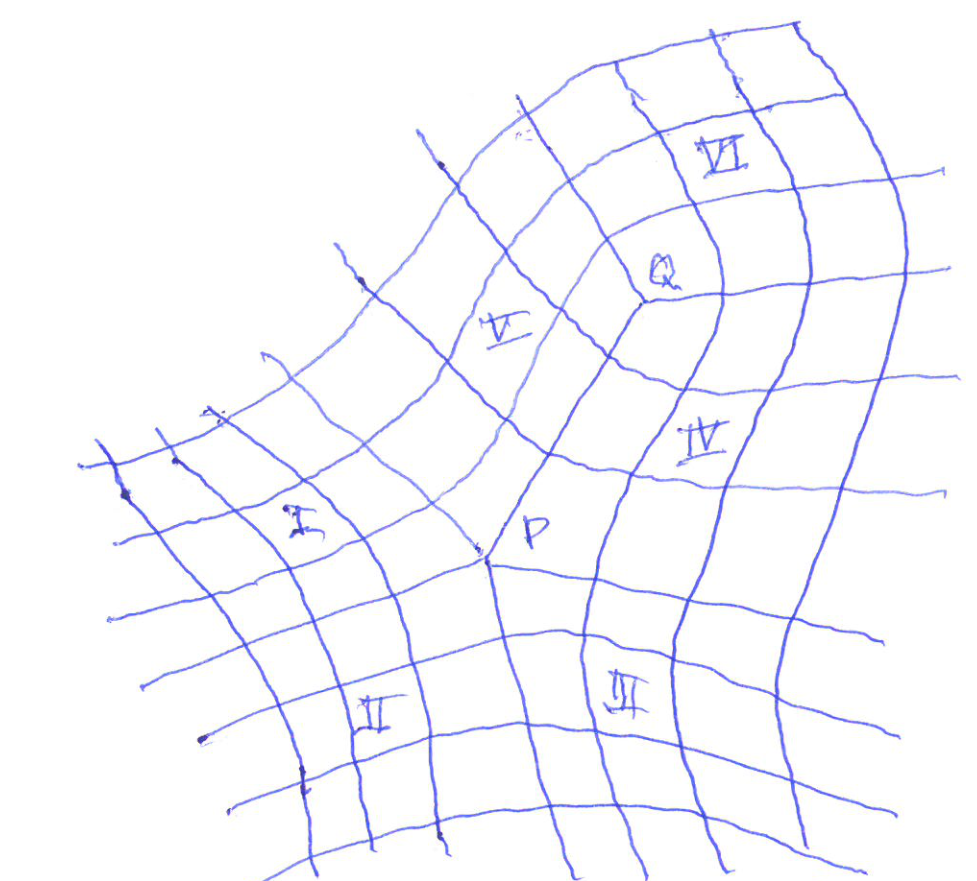
What is represented in this figure is the geometric offprint of a 2D-script which is unitary and tight. Hence the above figure determines the script up to equivalence. It appears to be a curved or bent 2D-surface with

• a curvature point $P$ with negative curvature $-1$

• a curvature point $Q$ with positive curvature $+1$

All the other points, lines, and spheres are like in the standard grid $\mathbb{Z}^{2}$ that is flat.

In Einstein’s theory, curvature is linked to gravity and in script geometry, curvature is a property of the geometric offprint alone, not of the actual script itself, that seems closer related to electromagnetism.

But of course we want to have at least one script for which this model is the geometric offprint we will realize it as 2D-surface inside $\mathbb{Z}^{3}$ where $\mathbb{Z}$ consists of points $a\in\{\ldots,-2,-1,0,1,2,\ldots\}$ and lines $I_{j},j\in\mathbb{Z}$ with $\partial I_{j}="j+1"-"j"$. Hence, in $\mathbb{Z}^{3}$ itself we have points $(a_{1},a_{2},a_{3})\in\mathbb{Z}^{3}$, lines $(I_{j},a_{2},a_{3}),(a_{1},I_{j},a_{3}),(a_{1},a_{2},I_{j})$ with e.g. $\partial(I_{j},a_{2},a_{3})=(j+1,a_{2},a_{3})-(j,a_{2},a_{3})$ and planes $(I_{j},I_{k},a_{3})$, $(I_{j},a_{2},I_{k})$, $(a_{1},I_{j},I_{k})$ with e.g. $\partial(I_{j},I_{k},a_{3})=(j+1,I_{k},a_{3})-(j,I_{k},a_{3})-(I_{j},k+1,a_{3})+(I_{j},k,a_{3})$ and volumes $(I_{j},I_{k},I_{l})$ but we won’t be needing theses.

Hence, the script equations follow from the cartesian product $\mathbb{Z}^{3}$ and all we have to do is to determine how the curvature model fits into $\mathbb{Z}^{3}$.

We have decomposed it into 6 overlapping zones consisting of points

• Zone 1: $(a_{1},a_{2},0)\;\&\;a_{1}\leq 0,a_{2}\geq 0$

• Zone 2: $(a_{1},a_{2},0)\;\&\;a_{1}\leq 0,a_{2}\leq 0$

• Zone 3: $(a_{1},a_{2},0)\;\&\;a_{1}\geq 0,a_{2}\leq 0$

• Zone 4: $(a_{1},0,a_{3})\;\&\;a_{1}\geq 0,a_{3}=0,1,2,3$

• Zone 5: $(0,a_{2},a_{3})\;\&\;a_{2}\geq 0,a_{3}=0,1,2,3$

• Zone 6: $(a_{1},a_{2},3)\;\&\;a_{1}\geq 0,a_{2}\geq 0$

Also the lines can be computed zone by zone, of course these will be overlapping.

This leads to the list:

• Lines in Zone 1:

  $$(I_{j},a_{2},0) \& j<0,a_{2}\geq 0$$

  $$(a_{1},I_{j},0) \& j\geq 0,a_{1}\leq 0$$

• Lines in Zone 2:

  $$(I_{j},a_{2},0) \& j<0,a_{2}\leq 0$$

  $$(a_{1},I_{j},0) \& j<0,a_{1}\leq 0$$

• Lines in Zone 3:

  $$(I_{j},a_{2},0) \& j\geq 0,a_{2}\leq 0$$

  $$(a_{1},I_{j},0) \& j<0,a_{1}\geq 0$$

• Lines in Zone 4:

  $$(I_{j},0,a_{3}) \& j\geq 0,a_{3}=0,1,2,3$$

  $$(a_{1},0,I_{j}) \& a_{1}\geq 0,j=0,1,2$$

• Lines in Zone 5:

  $$(0,I_{j},a_{3}) \& j\geq 0,a_{3}=0,1,2,3$$

  $$(0,a_{2},I_{j}) \& a_{2}\geq 0,j=0,1,2$$

• Lines in Zone 6:

  $$(I_{j},a_{2},3) \& j\geq 0,a_{2}\geq 0$$

  $$(a_{1},I_{j},3) \& j\geq 0,a_{1}\geq 0$$

Similarly, we have the plane elements (no overlapping)

• Planes in Zone 1:

  $$(I_{j},I_{k},0)\;;\;j<0\;\&\;k\geq 0$$

• Planes in Zone 2:

  $$(I_{j},I_{k},0)\;;\;j<0\;\&\;k<0$$

• Planes in Zone 3:

  $$(I_{j},I_{k},0)\;;\;j\geq 0\;\&\;k<0$$

• Planes in Zone 4:

  $$(I_{j},0,I_{k})\;;\;j\geq 0\;\&\;k=0,1,2$$

• Planes in Zone 5:

  $$(0,I_{j},I_{k})\;;\;j\geq 0\;\&\;k=01,2,3$$

• Planes in Zone 6:

  $$(I_{j},I_{k},3)\;;\;j\geq 0\;\&\;k\geq 0$$

This fixes the whole script because the script relations follow from the cartesian product. In script geometry much of the creativity lies in finding the best algorithms to describe something. Scripts also involve gravity and electromagnetism combined whereby everything is expressed in terms of chains and their supports.

6.6. The “simplicial” cartesian product

We again start from two scripts

$$S : 0\leftarrow\mathbb{Z}\leftarrow M_{0}(\mathcal{C}_{0})\overset{\partial}{\longleftarrow}\cdots$$

$$S^{\prime} : 0\leftarrow\mathbb{Z}\leftarrow M_{0}(\mathcal{C}_{0}^{\prime})\overset{\partial}{\longleftarrow}\cdots$$

Then the “simplicial” cartesian product is defined as the complex

$$S\times S^{\prime}:0\leftarrow\mathbb{Z}=M_{-2}({1})\overset{\partial}{\longleftarrow}M_{-1}(\mathcal{C}_{-1}^{\prime\prime})\overset{\partial}{\longleftarrow}M_{0}(\mathcal{C}_{0}^{\prime\prime})\overset{\partial}{\longleftarrow}\cdots$$

whereby this time for $k\geq-2$

$$\mathcal{C}_{k}^{\prime\prime}=\bigcup_{s=-1}^{k+1}\mathcal{C}_{s}\times\mathcal{C}_{k-s}^{\prime}$$

and as before

$$\mathcal{C}_{s}\times\mathcal{C}_{k-s}^{\prime}=\{(C_{j}^{s},C_{l}^{\prime,k-s}:\ldots)\}$$

so for example

$$\mathcal{C}_{-2}^{\prime\prime} = \{(1,1)\}=\{1\}$$

$$\mathcal{C}_{-1}^{\prime\prime} = \{(p_{j},1),(1,p_{j}^{\prime}):p_{j}\in\mathcal{C}_{0},p_{j}^{\prime}\in\mathcal{C}_{0}^{\prime}\}$$

$$\mathcal{C}_{0}^{\prime\prime} = \{(p_{j},p_{l}^{\prime}):p_{j}\in\mathcal{C}_{0},p_{j}^{\prime}\in\mathcal{C}_{0}^{\prime}\}\cup\{(1,l_{j}^{\prime}):l_{j}^{\prime}\in\mathcal{C}_{1}^{\prime}\}\cup\{(l_{j},1):l_{j}\in C_{j}\}$$

Just like before the $\partial$-operator is defined by

$$\partial(C_{j}^{s},C_{l}^{\prime,k-s})=(\partial C_{j}^{s},C_{l}^{\prime,k-s})+(-1)^{s}(C_{j}^{s},\partial C_{l}^{\prime,k-s})$$

whereby this time $s\geq-1,k\geq-2$.

So for example

$$\partial(p_{j},1) = (1,1)=1$$

$$\partial(1,p_{j}^{\prime}) = -(1,\partial p_{j}^{\prime})=-(1,1)=-1$$

$$\partial(p_{j},p_{l}^{\prime}) = (1,p_{l}^{\prime})+(p_{j},1)$$

$$\partial(1,l_{j}^{\prime}) = -1(1,\partial l_{j}^{\prime})=-(1,p_{\alpha}^{\prime}-p_{\beta}^{\prime})$$

and so on.

So the main difference with the cubic case is that we make explicit use of the accumulations of $S$ and $S^{\prime}$ within the $\partial$-operator. This means that we have extra cells

$$(C_{j}^{k},1),(1,C_{j}^{\prime,k}).$$

Also the elements $(p_{j},p_{l}^{\prime})$ behave like lines rather than points while the sets

$$\mathcal{C}_{0}\times\{1\}=\{(p_{j},s):\cdots\},\{1\}\times\mathcal{C}_{0}^{\prime}=\{(1,p_{j}^{\prime}):\cdots\}$$

are like two sets of points for which

$$\partial(p_{j},1)=1,\partial(1,p_{j}^{\prime})=-1.$$

This may seem questionable because normally the boundary of a point is +1. But one can always introduce $-(1,p_{j}^{\prime})$ as “new points”. Also the dimensions of cells seem to have a shift $-1$, it is

$$\mathrm{dim}1=-2,\qquad\mathrm{dim}(p_{j},1)=-1,\qquad\mathrm{dim}(p_{j},p_{l}^{\prime})=0.$$

while one would rather expect

$$\mathrm{dim}1=-1,\qquad\mathrm{dim}(p_{j},1)=0,\qquad\mathrm{dim}(p_{j},p_{l}^{\prime})=1.$$

One can of course redefine the dimensions of the cells in this way. But that gives problems when defining longer symplicial cartesian products like $S_{1}\times S_{2}\times\ldots\times S_{l}$,

$$S_{j} : 0\leftarrow\mathbb{Z}\leftarrow M_{0}(\mathcal{C}_{0,j})\overset{\partial}{\longleftarrow}\ldots$$

$$\times_{j=1}^{l}S_{j} : 0\leftarrow\mathbb{Z}=M_{-l}(\mathcal{C}_{-l}^{\prime\prime})\overset{\partial}{\longleftarrow}M_{-l+1}(\mathcal{C}_{-l+1}^{\prime\prime})\leftarrow\ldots\overset{\partial}{\longleftarrow}M_{0}(\mathcal{C}_{0}^{\prime\prime})\leftarrow\ldots$$

whereby for $k\geq-l$

$$\mathcal{C}_{k}^{\prime\prime}=\bigcup_{k_{1}+\ldots+k_{l}=k}\mathcal{C}_{k_{1},1}\times\ldots\times\mathcal{C}_{k_{l},l}$$

and the boundary operators is still given by

$$\partial(C_{j_{1}}^{k_{1},1},\ldots,C_{j_{l}}^{k_{l},l})$$

$$= (\partial C_{j_{1}}^{k_{1},1},\ldots,C_{j_{l}}^{k_{l},l})+\ldots+(-1)^{k_{1}+\ldots+k_{l}}(C_{j_{1}}^{k_{1},1},\ldots,\partial C_{j_{l}}^{k_{l},l}),\quad k_{1},\ldots,k_{l}=-1,0,\ldots.$$

Again, one can consider the elements

$$(p_{j}^{1},1,\ldots,1),(1,p_{j}^{2},\ldots,1),\ldots,(1,\ldots,p_{j}^{l})$$

as a partition of the whole set of points and one could redefine the dimension of objects

$$\mathrm{dim}(\mbox{ object })\rightarrow\mathrm{dim}(\mbox{ object })+l-1$$

to be in agreement with the general theory of scripts and to renormalize the points, lines, etc. so that $\partial$ point$=+1$. But these are rather cosmetic changes one does not need to make.

Example 6.6.1.

Let

$$S:0\leftarrow\mathbb{Z}\leftarrow M_{0}(\{p\})$$

the script of a single point. Then $S\times S\times S\times S$ has cells

$$k=-4 : (1,1,1,1)=1$$

$$k=-3 : (p,1,1,1),(1,p,1,1),(1,1,p,1),(1,1,1,p)$$

$$k=-2 : (p,p,1,1),(p,1,p,1),(p,1,1,p),(1,p,p,1),(1,p,1,p),(1,1,p,p)$$

$$k=-1 : (p,p,p,1),(p,p,1,p),(p,1,p,p),(1,p,p,p)$$

$$k=0 : (p,p,p,p)$$

The boundary map in this script follows from the general theory. For example,

$$\partial(1,p,1,1) = -1$$

$$\partial(p,1,p,1) = (1,1,p,1)-(p,1,1,1)$$

$$\partial(p,p,1,p) = (1,p,1,p)+(p,1,1,p)-(p,p,1,1),\mbox{ etc. }$$

The geometric offprint of this script is the same as that of a symplex (up to dimensional shift). Hence, the script is tight and hence the script is equivalent to a symplex.

Exercise 6.6.1.

Let $S:0\leftarrow\mathbb{Z}\leftarrow M_{0}(\{p,q\})\leftarrow M_{1}(\{l\}),\partial l=p-q.$. Prove that $S\times S$ is also a 3D symplex.

Concerning tightness we have:

Theorem 6.6.1.

Let $S_{1},S_{2}$ be tight scripts then the symplicial cartesian product $S_{1}\times S_{2}$ is also tight.

Proof.

Adapt the cubic case (exercise). ∎

A similar result holds for $S_{1}\times S_{2}\times\ldots\times S_{l}$; in fact one can use associativity $(S_{1}\times S_{2})\times S_{3}=S_{1}\times(S_{2}\times S_{3})=S_{1}\times S_{2}\times S_{3}$.

6.7. The simplicial refinement

In this subsection we start from a script

$$S:0\leftarrow\mathbb{Z}\leftarrow M_{0}\overset{\partial}{\longleftarrow}\ldots$$

and first consider the $1$-point script $P$

$$C_{0}=\{p\},\partial p=1.$$

The idea is to construct a canonical symplicial complex such that to every cell $C_{j}^{k}$ corresponds a unique chain of symplexes $\sigma(C_{j}^{k})$ so that $\mbox{\kern-13.00005pt{ b}}(\partial C_{j}^{k})=supp\partial^{2}C_{j}^{k}=\{0\}$ which implies $\partial\sigma(C_{j}^{k})=\sigma(\partial C_{j}^{k})$, i.e. the script can be replaced via $\sigma$ by a symplicial complex.

The idea is based on the idea that, within $S\times P$,

$$\partial(C_{j}^{k},p)=(\partial C_{j}^{k},p)+(-1)^{k}(C_{j}^{k},1)$$

so that $(C_{j}^{k},1)$ is cobordant with $(-1)^{k-1}(C_{j}^{k},p)$.

The algorithm is recursive and goes in stages.

• Stage 0: Identify $S$ with $(S,1)$ consisting of cells $(C_{j}^{k},1)$ of which the dimension is shifted to $k-1$. In particular $(1,1)$ has dimension $-2$. Next for every point $(p_{j},1)\in(S,1)$ we put $\sigma(p_{j},1)=-(1,p_{j})$.

• Stage $k$: Suppose that we have completed stage $k-1$ and let $(C_{j}^{k},1)\in(C^{k},1)$. For each such element we create a new point $p_{j}^{k}$ and define

  $$\sigma(C_{j}^{k})=(-1)^{k-1}(\partial C_{j}^{k},p_{j}^{k})\sim(C_{j}^{k},1)$$

  where $\sim$ denotes the cobordism.

  The dimensions are the same, it is a chain of symplexes because $\partial C_{j}^{k}=\sum$ symplexes and (symplex, point) is a symplex.

  Also $\partial\sigma(C_{j}^{k})=(\partial C_{j}^{k},\partial p_{j}^{k})=(\partial C_{j}^{k},1)=\sigma(\partial C_{j}^{k})$ whatever. Finally for every $C_{j}^{k+1}$, if $C_{l}^{k}$ occurs in $\partial C_{j}^{k+1}$, replace $C_{j}^{k}$ by $\sigma(C_{l}^{k})$ and raise the dimension of $\sigma(C_{l}^{k})$ by $+1$.

• Last stage: Cancel all elements $(C_{j}^{k},1)$.

Example 6.7.1.

Consider the disc $C_{0}=\{p_{1},p_{2}\},C_{1}=\{l_{1},l_{2}\},C_{2}=\{v\},\partial l_{1}=\partial l_{2}=p_{2}-p_{1},\partial v=l_{2}-l_{1}$. First we are to replace $p_{j}\rightarrow-(1,p_{j})$ then $\partial l_{1}=\partial l_{2}=-(1,p_{2})+(1,p_{1})$. Next we introduce points $q_{1},q_{2}$ then we replace

$$\sigma:l_{j}\rightarrow+(-(1,p_{2})+(1,p_{1}),q_{j})=-((1,p_{2}),q_{j})+((1,p_{1}),q_{j})$$

now we replace

$$\partial v=l_{2}-l_{1}\rightarrow-((1,p_{2}),q_{2})+((1+p_{1}),q_{2})+((1,p_{2}),q_{1})-((1,p_{1}),q_{1}).$$

So taking new point $q$, we obtain

$$\sigma:v\rightarrow-((1,p_{2}),q_{2})+((1,p_{1}),q_{2})+((1,p_{2}),q_{1})-((1,p_{1},q_{1}),q);$$

it is the sum of 4 triangles

Figure 6.7.1. Simplicial refinement of two lines

It is important to know that every script can be refined to a simplicial complex. Note that the refinement of the sphere $S^{2}$ is an octahedron. For higher dimensions: similar story.

Affilations

Paula Cerejeiras
CIDMA - Center for Research and Development in Mathematics and Applications, Department of Mathematics,University of Aveiro, Campus Universitário de Santiago, 3810-193 Aveiro, Portugal
pceres@ua.pt

Uwe Kähler
CIDMA - Center for Research and Development in Mathematics and Applications, Department of Mathematics,University of Aveiro, Campus Universitário de Santiago, 3810-193 Aveiro, Portugal
ukaehler@ua.pt

Teppo Mertens
Clifford Research Group, Department of Mathematical Analysis, Ghent University, Galglaan 2, B-9000 Ghent, Belgium
teppo.mertens@ugent.be

Frank Sommen
Clifford Research Group, Department of Mathematical Analysis, Ghent University, Galglaan 2, B-9000 Ghent, Belgium
frank.sommen@ugent.be

Adrian Vajiac
CECHA - Center of Excellence in Complex and Hypercomplex Analysis, Chapman University, One University Drive, Orange CA 92866
avajiac@chapman.edu

MihaelaVajiac
CECHA - Center of Excellence in Complex and Hypercomplex Analysis, Chapman University, One University Drive, Orange CA 92866
mbvajiac@chapman.edu

References

- [1] D.N. Arnold, R.S. Falk, R. Winther, Finite element exterior calculus, homological techniques, and applications, Acta Numer. 15 (2006), 1-155.
- [2] D.N. Arnold, R.S. Falk, R. Winther, Finite element exterior calculus: from Hodge theory to numerical stability, Bull., New Ser., Am. Math. Soc. 47 (2010) 2, 281-354.
- [3] A. Bossavit, Whitney forms: a class of finite elements for three-dimensional computations in electro-magnetism, IEE Proc. A, Sci. Meas. Technol. 135 (1988) 8, 493-500.
- [4] P. Cerejeiras, U. Kähler, D. Legatiuk, Finite element exterior calculus with script geometry, International Conference of Numerical Analysis and Applied Mathematics 2019, ICNAAM 2019, AIP Conference Proceedings, Theodore E. Simos and Charalambos Tsitouras, 1-3, Rhodes; Greece, 2019.
- [5] P. Cerejeiras, U. Kähler, F. Sommen, A. Vajiac, Script Geometry, in: S. Bernstein, U. Kähler, I. Sabadini F. Sommen, Modern Trends in Hypercomplex Analysis, Birkhäuser, Basel, 2016, 79-110.
- [6] M. Desbrun, E. Kanso, Y. Tong, Discrete Differential Forms for Computational Modelling, in Discrete Differential Geometry, edt. A.I. Bobenko, J.M. Sullivan, P. Schröder, G.M. Ziegler, Birkäuser, Basel, 2008, 287-324
- [7] M. Holst, A. Stern, Geometric variational crimes: Hilbert complexes, finite element exterior calculus, and problems on hypersurfaces, Foundations of Computational Mathematics, 12 (2012), 263-293.
- [8] A. Stern, P. Leopardi, The abstract Hodge-Dirac operator and its stable discretization, SIAM Journal on Numerical Analysis, 54 (2016) 6, 3258–3279.
- [9] H. Whitney, Geometric Integration Theory, Princeton University Press, Princeton, NJ, 1957.