Particle physics model of curvaton inflation
in a stable universe

Abstract

We investigate a particle physics model for cosmic inflation based on the following assumptions: (i) there are at least two complex scalar fields; (ii) the scalar potential is bounded from below and remains perturbative up to the Planck scale; (iii) we assume slow-roll inflation with maximally correlated adiabatic and entropy fluctuations 50–60 e-folds before the end of inflation. The energy scale of the inflation is set automatically by the model. Assuming also at least one massive right handed neutrino, we explore the allowed parameter space of the scalar potential as a function of the Yukawa coupling of this neutrino.

I Introduction

The precise mechanism of cosmic inflation is one of the most pressing questions in our understanding of the early universe. Today the original idea for inflation [1] is not favoured because it is unclear how to define a proper mechanism to explain the required reheating of the universe. A popular solution to this question of reheating is the slow-roll scenario [2, 3] in which the ground state starts from an unstable position and rolls down very slowly to a local or global minimum. The inflation stops when the potential energy function becomes too steep, which leads to a fast roll. In principle, the slow roll can start from a large field value and proceed towards a minimum with a smaller field value, or from a small (essentially vanishing) field value to a larger minimum. These two cases are referred to as large- and small-field slow roll [4]. A problem related to large-field slow-roll is the initial value problem, namely one has to explain why the ground state starts from a value much larger than the typical energy scale of inflation. Chaotic inflation [5] was devised to handle this problem, but then one has to assume very large – again larger than the scale of inflation – fluctuations. The origin of inflation is still an open question in cosmology [6, 7].

It is known that scalar fields can mimic the equation of state required for the exponential expansion of the early universe [2, 3]. As the Higgs boson was discovered [8, 9], we know that at least one doublet scalar field exists in nature. Hence, it may appear natural to assume that the Brout-Englert-Higgs (BEH) field is the inflaton (see for example LABEL:Bezrukov:2014ipa), but such a scenario was criticised, see for instance LABEL:Martin:2013tda. Many types of scalar potentials have already been discussed in the literature as viable scenarios for cosmic inflation [11]. There are three major categories of scalar inflaton potentials with minimal kinetic terms: (i) the large field, (ii) the small field and (iii) the hybrid models. In the third case one introduces more than one field, with one of those being the inflaton and the other field switches off the exponential expansion. In this sense it is not a real multifield model. The case of hybrid models is excluded by experimental observations because those predict a scalar tilt $n_{s}$ larger than one in contradiction with the observed structure of the thermal fluctuations of the cosmic microwave background radiation (CMBR) resulting in $n_{s}=0.9677\pm 0.0060$ [12, 13]. The tensor and scalar power spectra of the CMBR suggest a small value for the tensor-to-scalar ratio $r$, consistent with zero, which emerges automatically in real multifield models with curvaton scenario [14, 15, 16, 17].

In this letter we consider a simple multifield particle physics model of cosmic inflation with a curvaton scenario. We show that in a fairly constrained region of the parameter space, the model can provide a natural switch on and off mechanism of inflation.

II Particle physics model

The particle content of the model coincides with that in the standard model of particle interactions, supplemented with one complex scalar field. We also allow for one (or more) Dirac-, or Majorana-type right-handed neutrinos. In this letter for the sake of definiteness we consider the case of Dirac neutrinos.

In addition to the usual $SU(2)$-doublet scalar field

$$\phi=\left(\!\!\begin{array}[]{c}\phi^{+}\\ \phi^{0}\end{array}\!\!\right)=\frac{1}{\sqrt{2}}\left(\!\!\begin{array}[]{c}\phi_{1}+\mathrm{i}\phi_{2}\\ \phi_{3}+\mathrm{i}\phi_{4}\end{array}\!\!\right)\,,$$ (1)

we assume the existence of a complex scalar $\chi$ that transforms as a singlet under the standard model gauge transformations. The potential energy of these scalar fields is assumed as

$$V(\phi,\chi)=V_{0}-\mu_{\phi}^{2}|\phi|^{2}-\mu_{\chi}^{2}|\chi|^{2}+\frac{1}{2}\left(|\phi|^{2},|\chi|^{2}\right)C\left(\!\!\begin{array}[]{c}|\phi|^{2}\\ |\chi|^{2}\end{array}\!\!\right)$$ (2)

where $|\phi|^{2}=|\phi^{+}|^{2}+|\phi^{0}|^{2}$ and $C=\left(\!\!\begin{array}[]{cc}2\lambda_{\phi}&\lambda\\ \lambda&2\lambda_{\chi}\end{array}\!\!\right)$ is the coupling matrix. This potential energy function contains a coupling term $\lambda|\phi|^{2}|\chi|^{2}$ of the scalar fields in addition to the usual quartic terms. The value of the additive constant $V_{0}$ is irrelevant for particle dynamics, but as we shall see, it is relevant for the inflationary model, hence we allow a non-vanishing value for it. In order that this potential energy be bounded from below, we have to require the positivity of the self-couplings, $\lambda_{\phi}$, $\lambda_{\chi}>0$, and also the coupling matrix be positive definite,

$${\det}_{C}=4\lambda_{\phi}\lambda_{\chi}-\lambda^{2}>0\,,\textrm{ if }\lambda<0\,.$$ (3)

Our model for cosmic inflation works only if $\lambda<0$. If these conditions are satisfied, we find the minimum of the potential energy at field values $\phi=v$ and $\chi=w$ where the vacuum expectation values (VEVs) are

$$v=\sqrt{\frac{2\lambda_{\chi}\mu_{\phi}^{2}-\lambda\mu_{\chi}^{2}}{4\lambda_{\phi}\lambda_{\chi}-\lambda^{2}}}\,,\qquad w=\sqrt{\frac{2\lambda_{\phi}\mu_{\chi}^{2}-\lambda\mu_{\phi}^{2}}{4\lambda_{\phi}\lambda_{\chi}-\lambda^{2}}}\,.$$ (4)

Using the VEVs, we can express the quadratic couplings as

$$\mu_{\phi}^{2}=2\lambda_{\phi}v^{2}+\lambda w^{2}\,,\qquad\mu_{\chi}^{2}=2\lambda_{\chi}w^{2}+\lambda v^{2}\,.$$ (5)

For $\lambda<0$, the constraint (3) ensures that the denominators of the VEVs in Eq. (4) are positive, so the VEVs have non-vanishing real values only if the inequalities

$$2\lambda_{\chi}\mu_{\phi}^{2}-\lambda\mu_{\chi}^{2}>0\quad\text{and}\quad 2\lambda_{\phi}\mu_{\chi}^{2}-\lambda\mu_{\phi}^{2}>0$$ (6)

are satisfied simultaneously, which can be fulfilled [19] if at most one of the quadratic couplings is smaller than zero .

After spontaneous symmetry breaking and choosing unitary gauge, the scalar kinetic term leads to a mass matrix of the two real scalars . We can diagonalize this matrix by an orthogonal rotation and find for the masses $M_{h/H}$ of the mass eigenstates:

$$\frac{M_{h/H}^{2}}{2}=\lambda_{\phi}v^{2}+\lambda_{\chi}w^{2}\mp\sqrt{(\lambda_{\phi}v^{2}-\lambda_{\chi}w^{2})^{2}+(\lambda vw)^{2}}$$ (7)

where $M_{h}\leq M_{H}$ by convention. At this point either $h$ or $H$ can correspond to the observed scalar boson. As $M_{h}$ must be positive, the condition

$$v^{2}w^{2}\Big{(}4\lambda_{\phi}\lambda_{\chi}-\lambda^{2}\Big{)}>0$$ (8)

has to be fulfilled. If both VEVs are greater than zero, as needed for two non-vanishing scalar masses, then this condition coincides with the positivity constraint (3).

We studied the ultraviolet behaviour of the scalar couplings of this model in LABEL:Peli:2019xwv where we constrained the parameter space by requiring that (i) the scalar potential remains bounded from below and (ii) the couplings remain perturbative up to the Planck scale $m_{P}$.

III Cosmological inflation

We now explore the cosmic inflation of the two-field model with potential energy defined in Eq. (2). We consider slow-roll inflation when the potential energy has a large, almost flat area for small field values and a global minimum at large values of the VEVs. Such a potential energy allows for slow roll of the fields from small values towards the global minimum, resulting in cosmic inflation. The required form of the potential energy function appears naturally at some high energy scale, for certain values of the scalar couplings at the mass of the t-quark $m_{\mathrm{t}}$. As Eq. (4) shows, the VEVs are inversely proportional to $\sqrt{{\det}_{C}}$. Fig. 1 shows the running of ${\det}_{C}$ together with that of the couplings from initial values at $m_{\mathrm{t}}$ chosen from the stability region. We see a narrow wedge – like an inverse resonance – where ${\det}_{C}$ becomes very small, implying VEVs at around field values of $10^{5}$ GeV. The figure shows an example with vanishing Yukawa coupling $c_{\nu}$ of the right-handed neutrino, but below we show that the value of $c_{\nu}$ influences only the size of the parameter space of the scalar couplings where this phenomenon leads to such potential energy function that can support cosmic inflation in accordance with current values of relevant observables.

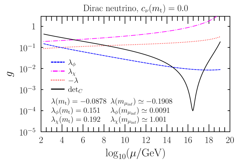
Figure 1: Running of the scalar couplings and of ${\det}_{C}$. $g$ means any of the couplings.

The single-field inflationary models predict purely curvature perturbations, resulting from energy density fluctuations. Having multiple fields allows for multiple types of fluctuations, hence several observable quantities, such as the tilts corresponding to curvature, isocurvature (emerging due to fluctuations in the relative number density of particles) and a correlation angle $\Delta$ [22].

Following LABEL:Gordon:2000hv, we introduce a local rotation of $(\phi,\chi)$ into $(\sigma,s)$ where $\sigma$ refers to the adiabatic field and $s$ to the entropy field. The adiabatic field is the path length along the classical trajectory, while $s$ remains a constant. The number of slow-roll parameters also increase. In the single-field case, in addition to the parameter $\epsilon$ describing the deviation from the equation of state of the de-Sitter space-time, $\epsilon=\frac{3}{2}\left(\frac{\displaystyle p}{\displaystyle\rho}+1\right)$, there is only one other slow roll parameter $\eta$, which essentially measures the acceleration of the fields. In our example we have three $\eta$ parameters that can be expressed approximately from the potential as

$$\eta_{ij}\simeq m_{p}^{2}\frac{\partial_{ij}V}{V}\,,\quad ij=\phi\phi,\>\chi\chi,\>\phi\chi,\>ss,\>\sigma\sigma,\>s\sigma$$ (9)

(note that $\eta_{\phi\phi}+\eta_{\chi\chi}=\eta_{\sigma\sigma}+\eta_{ss}$), while

$$\epsilon\simeq\frac{1}{2}m_{P}^{2}\biggl{(}\frac{\partial_{\sigma}V}{V}\biggr{)}^{2}\,.$$ (10)

In principle, inflation is possible only until both $\epsilon$ and $\eta_{ij}$ are small, resulting in the slow roll.

To set the exact conditions of slow roll, we solved the equations of motion with the integration variable transformed to the number of e-folds $N$, and terminated the process, when either of the slow-roll parameters reached unity. We set the starting point of the trajectory at vanishing field values. For the parameter values of the potential energy we used values allowed by the perturbativity and stability conditions mentioned in the section describing the model, namely $|\lambda|,\>\lambda_{i}\sim\mathrm{O}(10^{-1}-10^{-2})$ and $\mu_{i}^{2}/\mathrm{GeV}^{2}\sim\mathrm{O}(1-3\times 10^{4})$. For such values we have found that the $\eta_{ij}$ parameters increase much faster than $\epsilon$, reaching 1, while $\epsilon$ remaining small, about $\mathrm{O}(10^{-30})$. Hence, we set the end of inflation by the condition $\eta_{ij}=1$. In practice the parameter $\eta_{\chi\chi}$ increases the fastest. We show an example of such a trajectory in Fig. 2. This trajectory induces $N>200$ e-folds. The value of $\eta_{ss}^{*}$ refers to the value of $\eta_{ss}$ at $60$ e-folds before the end of inflation.

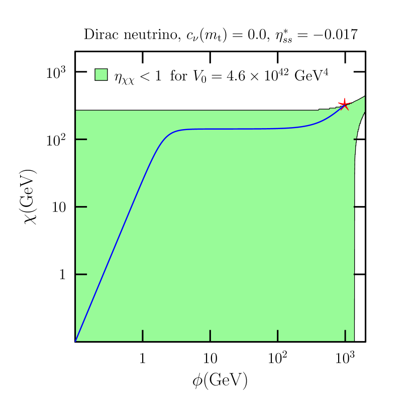
Figure 2: A possible trajectory of the rolling of the scalar fields.

The observables are constructed from the slow-roll parameters taken $50-60$ e-folds before the end of inflation. This corresponds to an even smaller $\epsilon$, which reduces the tensor-to-scalar ratio, $r=16\epsilon(\sin\Delta)^{2}$ to essentially zero. Such a small $r$ is not excluded by cosmological measurements. The smallness of $r$ however is in conflict with the traditional cosmological normalization

$$V_{0}\simeq r\left(1.6\cdot 10^{16}\text{ GeV}\right)^{4}\,.$$ (11)

This conflict may be resolved by assuming that the adiabatic and entropy fluctuations were maximally correlated at $50-60$ e-folds before the end of inflation, implying $\cos\Delta=1$, and hence predicting zero for the tensor-to-scalar ratio. Consequently, we have to find different conditions to set the scale of inflation $\mu_{\mathrm{inf}}$ and for the normalization of the potential energy. As suggested above, we provide the first from the particle physics model by identifying $\mu_{\mathrm{inf}}$ with the location of the wedge in the running of ${\det}_{C}$. The case of $\Delta=0$, i.e. maximally correlated fluctuations are referred to as the curvaton scenario. In this case, the various tilts coincide. Neglecting $\epsilon$, we have:

$$n_{s}-1=2\eta_{ss}$$ (12)

Considering $\eta_{ss}$ as a function of $V_{0}$ (see Eq. (9) with $V_{0}$ in $V$ in the denominator), we normalize it to produce the scalar tilt in agreement with the most recent data, $n_{s}\simeq 0.966$, yielding $V_{0}\simeq 5\times 10^{42}\,\mathrm{GeV}^{4}$.

Having fixed the value of $V_{0}$, we propose the following inflationary scenario. The scalar potential energy is given by Eq. (2). After the Big Bang the characteristic energy scale of particle interactions is near the Planck scale, hence the scalar fields are fluctuating around zero. As the universe expands, the characteristic energy scale decreases and the scalar couplings run according to their renormalization group equations, exhibiting the wedge for ${\det}_{C}$ at a scale $\mu_{\mathrm{inf}}$ (around $10^{16}\,$GeV) that we identify with the scale of inflation. At this scale the global minimum of the potential energy function increases to about $10^{5}$ GeV and the fields start to roll slowly towards this minimum, resulting in cosmic inflation. This accelerated expansion continues until the acceleration (second time derivative of the fields) remain negligible in the equation of the motion, determined by $\max\eta_{ij}=1$. The universe starts its Hubble expansion, decreasing the characteristic energy scale, and the global minimum of the scalar potential quickly returns to small field values.

IV Predicting the scalar couplings

The cosmological inflation as described in the previous section occurs only in a restricted region of the parameter space of the scalar couplings, which we define at the electroweak scale ($m_{\mathrm{t}}$).

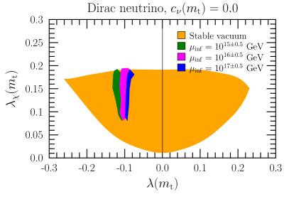
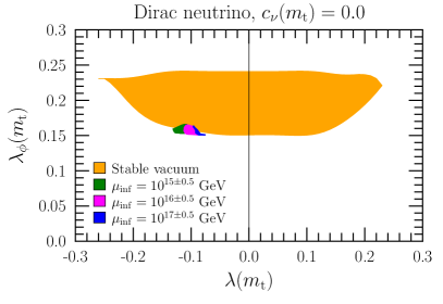
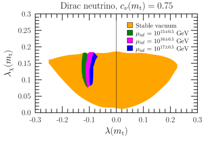
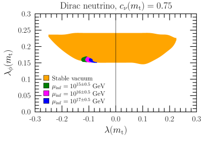
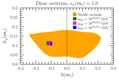
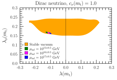
Figure 3: Projections of the allowed regions of the parameter space of scalar couplings onto the $\lambda-\lambda_{\chi}$ plane (left) and $\lambda-\lambda_{\phi}$ plane (right) at three different ranges of the scale of inflation and at three selected values of the $c_{\nu}$ Yukawa coupling.

The wedge in the running of ${\det}_{C}$ appears only for $\lambda(m_{\text{t}})<0$. We have scanned this side of the parameter space by selecting fixed initial values for the scalar couplings $\lambda_{\phi}(m_{\text{t}})$, $\lambda_{\chi}(m_{\text{t}})$, and scanning the allowed initial values of the third one to find those points where the wedge in the running of ${\det}_{C}$ appears with a minimum $\lesssim\mathrm{O}(10^{-4})$. During this scanning, we need to search only for those points where $w(m_{\mathrm{t}})$ – given by [19] $w(m_{\mathrm{t}})=2v(m_{\mathrm{t}})\sqrt{\frac{\displaystyle{\lambda}_{\rm SM}(m_{\mathrm{t}})(\lambda_{\phi}(m_{\mathrm{t}})-{\lambda}_{\rm SM}(m_{\mathrm{t}}))}{\displaystyle(4(\lambda_{\phi}(m_{\mathrm{t}})-{\lambda}_{\rm SM}(m_{\mathrm{t}}))\lambda_{\chi}(m_{\mathrm{t}})-\lambda(m_{\mathrm{t}})^{2})}}$, with ${\lambda}_{\rm SM}(m_{\mathrm{t}})=\frac{1}{2}m_{H}(m_{\mathrm{t}})^{2}/v(m_{\mathrm{t}})^{2}\simeq 0.126$ – and the masses of the scalars given by Eq. (7) remain positive. We find that the parameter space is constrained to a shell on the surface of the region allowed by the conditions of stability and perturbativity of $V$. The width of the shell is affected by the allowed depth of the minimum of ${\det}_{C}$: the smaller ${\det}_{C}$, the thinner the shell. Furthermore, we have also found that the minimum value of the location of the wedge $\mu_{\mathrm{inf}}$ is around $10^{14}$ GeV, depending slightly on $c_{\nu}(m_{\text{t}})$.

In Fig. 3 we present the results of such scan of the parameter space. These plots show different planar projections of the three dimensional parameter space, spanned by $\lambda_{\phi}(m_{\text{t}}),\lambda_{\chi}(m_{\text{t}})$ and $\lambda(m_{\text{t}})$. The shape and size of the supported regions is affected by the choice of $c_{\nu}(m_{\text{t}})$, as seen in the titles of the figures. We find that the parameter space of the scalar couplings is not empty, but constrained strongly if we assume that cosmic inflation took place as described above. This assumption constrains the smallest value of $w$ to around 265 GeV.

V Conclusions

In this letter we proposed a particle physics model of cosmic inflation. It requires at least two scalar fields. We found that in a small region of the parameter space of the scalar couplings, the determinant of the scalar quartic coupling matrix becomes very small at a scale around $10^{16}$ GeV. As a result the global minimum of the scalar potential increases significantly, allowing for an accelerated expansion of the universe by a slow-roll model at this scale, called the scale of inflation. We assume the curvaton scenario of inflation, i.e. maximally correlated adiabatic and entropy fluctuations at $50-60$ e-folds before the end of inflation, which implies vanishing tensor-to-scalar ratio. To set the normalization of the potential at vanishing field values, we required that the model reproduces the measured value of the scalar tilt. The inflation stops when the parameter that measures the acceleration of the fields starts to increase quickly. After this the global minimum of the potential decreases preventing the appearance of another period of inflation.