Duality and sensitivity analysis of multistage linear stochastic programs

Abstract

In this paper we investigate the dual of a Multistage Stochastic Linear Program (MSLP) to study two related questions for this class of problems. The first of these questions is the study of the optimal value of the problem as a function of the involved parameters. For this sensitivity analysis problem, we provide formulas for the derivatives of the value function with respect to the parameters and illustrate their application on an inventory problem. Since these formulas involve optimal dual solutions, we need an algorithm that computes such solutions to use them, i.e., we need to solve the dual problem.

In this context, the second question we address is the study of solution methods for the dual problem. Writing Dynamic Programming equations for the dual, we can use an SDDP type method, called Dual SDDP, which solves these Dynamic Programming equations computing a sequence of nonincreasing deterministic upper bounds on the optimal value of the problem. However, applying this method will only be possible if the Relatively Complete Recourse (RCR) holds for the dual. Since the RCR assumption may fail to hold (even for simple problems), we design two variants of Dual SDDP, namely Dual SDDP with penalizations and Dual SDDP with feasibility cuts, that converge to the optimal value of the dual (and therefore primal when there is no duality gap) problem under mild assumptions. We also show that optimal dual solutions can be obtained computing dual solutions of the subproblems solved when applying Primal SDDP to the original primal MSLP.

The study of this second question allows us to take a fresh look at the class of MSLP with interstage dependent cost coefficients. Indeed, for this class of problems, cost-to-go functions are non-convex and solution methods were so far using SDDP for a Markov chain approximation of the cost coefficients process. For these problems, we propose to apply Dual SDDP with penalizations to the cost-to-go functions of the dual which are concave. This algorithm converges to the optimal value of the problem.

Finally, as a proof of concept of the tools developed, we present the results of numerical experiments computing the sensitivity of the optimal value of an inventory problem as a function of parameters of the demand process and compare Primal and Dual SDDP on the inventory and a hydro-thermal planning problems.

90C15, 90C90, 90C30

1 Introduction

Duality plays a key role in optimization. For generic optimization problems, weak duality allows to bound the optimal value. Dual information is also used in many optimization algorithms such as Uzawa algorithm [2], primal-dual projected gradient [21] or Stochastic Dual Dynamic Programming (SDDP) [22]. Moreover, for several classes of optimization problems, the dual is easier to solve than the primal problem, for instance when it is amenable to decomposition techniques such as price decomposition [4]. Even when there is a duality gap between the primal and dual optimal values, solving the dual already gives a bound on the optimal value, as mentioned earlier. Duality is also a fundamental tool in the reformulation of Robust Optimization problems, see for instance [3]. Finally, derivatives of the value function of classes of optimization problems can be related to optimal dual solutions, see [5], [24] and more recently [10, 12, 8] for the characterization of subdifferentials, subgradients, and $\varepsilon$-subgradients of value functions of convex optimization problems.

For stochastic control problems, stochastic Lagrange multipliers were already used in [16, 17, 18]. In the context of multistage stochastic programs, duality was studied in [26, 14], see also [28] for a review. More recently, the sensitivity analysis of multistage stochastic programs was discussed in [6] and [30]. In [6] the authors study the sensitivity with respect to parameters driving the considered price model. The corresponding parameters are in the objective function and the analysis of the estimate of marginal price is based on Danskin’s theorem with the SDDP method used for the numerical calculations. In [30], the authors use the Envelope Theorem for the sensitivity analysis. The required derivatives are described in terms of Lagrange multipliers associated with the value functions.

In this paper, focusing our attention on the dual of a Multistage Stochastic Linear Program (MSLP), we are able to provide insights into three important problems for MSLPs: sensitivity analysis, computation of a sequence of deterministic upper bounds on the optimal value which converges to the optimal value, and use of duality to solve Dynamic Programming (DP) equations on the dual which are simpler to solve (in the sense that they have convex cost-to-go functions) than primal DP equations for problems with interstage dependent cost coefficients. Our main contributions are summarized below.

Sensitivity analysis of MSLPs. We explain how to compute derivatives of the optimal value, seen as a function of the problem parameters, of a MSLP in terms of dual optimal solutions. Therefore, the construction of the dual problem is essential for our approach, contrary to [6]. With respect to the sensitivity analysis [30], in our approach, we do not use value functions directly, which are not known and can only be approximated, but rather construct the dual problem which is solved by an SDDP type algorithm, called Dual SDDP.

Writing Dynamic Programming equations for the dual problem. A simple but crucial ingredient for our developments and subsequent analysis of solution methods for the dual problem of a MSLP is to write DP equations for that dual problem. We are not aware of another paper with these equations. However, a similar study was done in [19]. More precisely, for a stochastic linear control problem with uncertainty in the right-hand-side, in [19], DP equations are written for the conjugate of the cost-to-go functions and using an SDDP type method for these DP equations, a sequence of upper bounds on the MSP optimal value is constructed which is the sequence of conjugate of the approximate first stage cost-to-go functions evaluated at the initial state $x_{0}$. Our approach has the advantage of being much simpler: contrary to derivations in [19] which require some algebra, our DP equations can be immediately obtained from the dual problem formulation, this latter being known (given in [28] for instance). On top of that, we relax two assumptions made in [19]: (a) the relatively complete recourse assumption of the dual and (b) randomness in the right-hand-side of the constraints only and interstage independent. The next three paragraphs describe how the scope of (a) and (b) was extended in our analysis.

Dual SDDP for dual problems without relatively complete recourse. In [19], it is assumed that the dual problem of the considered MSLP satisfies an assumption (Assumption 3) stronger than relatively complete recourse. This assumption may not be easy to check or may not be satisfied (for instance it is not satisfied for the inventory and hydro-thermal problems considered in Section 5). Therefore, it is desirable to extend the scope of Dual SDDP in such a way that it can still compute a deterministic converging sequence of upper bounds without this assumption. We present two variants of Dual SDDP that can do that: Dual SDDP with penalizations and Dual SDDP with feasibility cuts.

Dual SDDP for dual problems with all problem data random. Our DP equations are written for problems with uncertainty in all parameters. We explain how to apply Dual SDDP for such problems that do not satisfy (b) above.

Dual SDDP for problems with interstage dependent cost coefficients. Finally, we also relax assumption (b) considering problems having interstage dependent cost coefficients. Writing DP equations for the corresponding dual problem, we can apply Dual SDDP algorithm to solve these equations, which, interestingly, have concave cost-to-go functions whereas primal cost-to-go functions are not convex. This is in sharp contrast with the solution methods proposed so far such as [6, 20] which apply SDDP on the primal cost-to-go functions using a Markov chain approximation of the cost coefficients process.

The outline of the paper is the following. Our building blocks are elaborated in Section 2 where we write DP equations for the dual, we explain how to build upper bounding functions for the cost-to-go functions of the dual using penalizations, and study the dynamics of Lagrange multipliers. Sensitivity analysis of MSLPs is conducted in Section 3 while Dual SDDP and its variants are studied in Section 4. Finally, the results of numerical simulations testing the tools developed on an inventory and an hydro-thermal problem are presented in Section 5. The interested reader can find and test the code of all implementations and of Primal and Dual SDDP for MSLPs at https://github.com/vguigues/Dual_SDDP_Library_Matlab and https://github.com/vguigues/Primal_SDDP_Library_Matlab. Proofs are collected in the Appendix.

2 Duality of multistage linear stochastic programs

2.1 Writing Dynamic Programming equations for the dual

Consider the multistage linear stochastic program

(2.1) $$\begin{array}[]{cll}\min\limits_{x_{t}\geq 0}&{\mathbb{E}}\left[\sum_{t=1}^{T}c_{t}^{\top}x_{t}\right]\\ {\rm s.t.}&A_{1}x_{1}=b_{1},\\ &B_{t}x_{t-1}+A_{t}x_{t}=b_{t},\;t=2,...,T.\end{array}$$

Here vectors $c_{t}=c_{t}(\xi_{t})\in{\mathbb{R}}^{n_{t}}$, $b_{t}=b_{t}(\xi_{t})\in{\mathbb{R}}^{m_{t}}$ and matrices $B_{t}=B_{t}(\xi_{t})$, $A_{t}=A_{t}(\xi_{t})$ are functions of random process $\xi_{t}\in{\mathbb{R}}^{d_{t}}$, $t=1,...,T$ (with $\xi_{1}$ being deterministic). We denote by $\xi_{[t]}=(\xi_{1},...,\xi_{t})$ the history of the data process up to time $t$ and by ${\mathbb{E}}_{|\xi_{[t]}}$ the corresponding conditional expectation. The optimization in (2.1) is performed over functions (policies) $x_{t}=x_{t}(\xi_{[t]})$, $t=1,...,T,$ of the data process satisfying the feasibility constraints.

The Lagrangian of problem (2.1) is

(2.2) $$\begin{array}[]{l}L(x,\pi)={\mathbb{E}}\left[\sum_{t=1}^{T}c_{t}^{\top}x_{t}+\pi_{t}^{\top}(b_{t}-B_{t}x_{t-1}-A_{t}x_{t})\right]\end{array}$$

in variables $x=(x_{1}(\xi_{[1]}),\ldots,x_{T}(\xi_{[T]}))$ and $\pi=(\pi_{1}(\xi_{[1]}),\ldots,\pi_{T}(\xi_{[T]}))$ with the convention that $x_{0}=0$. Dualization of the feasibility constraints leads to the following dual of problem (2.1) (cf., [28, Section 3.2.3]):

(2.3) $$\begin{array}[]{cll}\max\limits_{\pi}&{\mathbb{E}}\big{[}\sum_{t=1}^{T}b_{t}^{\top}\pi_{t}\big{]}\\ {\rm s.t.}&A^{\top}_{T}\pi_{T}\leq c_{T},\\ &A_{t-1}^{\top}\pi_{t-1}+{\mathbb{E}}_{|\xi_{[t-1]}}\left[B_{t}^{\top}\pi_{t}\right]\leq c_{t-1},\;t=2,...,T.\end{array}$$

The optimization in (2.3) is over policies $\pi_{t}=\pi_{t}(\xi_{[t]})$, $t=1,...,T$.

Unless stated otherwise, we make the following assumption throughout the paper.

• The process $\xi_{1},...,\xi_{T}$ is stagewise independent (i.e., random vector $\xi_{t+1}$ is independent of $\xi_{[t]}$, $t=1,...,T-1$), and distribution of $\xi_{t}$ has a finite support, $\{\xi_{t1},\ldots,\xi_{tN_{t}}\}$ with respective probabilities $p_{tj}$, $j=1,...,N_{t}$, $t=2,...,T$. We denote by $A_{tj},B_{tj},c_{tj},b_{tj}$ the respective scenarios corresponding to $\xi_{tj}$.

Since the random process $\xi_{t}$, $t=1,...,T$, has a finite number of realizations (scenarios), problem (2.1) can be viewed as a large linear program and (2.3) as its dual. By the standard theory of linear programming we have the following.

Proposition 2.1.

Suppose that problem (2.1) has a finite optimal value. Then the optimal values of problems (2.1) and (2.3) are equal to each other and both problems have optimal solutions.

We can write the following dynamic programming equations for the dual problem (2.3). At the last stage $t=T$, given $\pi_{T-1}$ and $\xi_{[T-1]}$, we need to solve the following problem with respect to $\pi_{T}$:

(2.4) $$\begin{array}[]{cll}\max\limits_{\pi_{T}}&{\mathbb{E}}[b_{T}^{\top}\pi_{T}]\\ {\rm s.t.}&A_{T}^{\top}\pi_{T}\leq c_{T},\\ &A_{T-1}^{\top}\pi_{T-1}+{\mathbb{E}}\left[B_{T}^{\top}\pi_{T}\right]\leq c_{T-1}.\end{array}$$

Since $\xi_{T}$ is independent of $\xi_{[T-1]}$, the expectation in (2.4) is unconditional with respect to the distribution of $\xi_{T}$. In terms of scenarios the above problem can be written as

(2.5) $$\begin{array}[]{cll}\max\limits_{\pi_{T1},\ldots,\pi_{TN_{T}}}&\sum\limits_{j=1}^{N_{T}}p_{Tj}b_{Tj}^{\top}\pi_{Tj}\\ {\rm s.t.}&A_{Tj}^{\top}\pi_{Tj}\leq c_{Tj},\;j=1,...,N_{T},\\ &A_{T-1}^{\top}\pi_{T-1}+\sum\limits_{j=1}^{N_{T}}p_{Tj}B_{Tj}^{\top}\pi_{Tj}\leq c_{T-1}.\end{array}$$

The optimal value $V_{T}(\pi_{T-1},\xi_{T-1})$ and an optimal solution $(\bar{\pi}_{T1},\ldots,\bar{\pi}_{TN_{T}})$ of problem (2.5) are functions of vectors $\pi_{T-1}$ and $c_{T-1}$ and matrix $A_{T-1}$. And so on going backward in time, using the stagewise independence assumption, we can write the respective dynamic programming equations for $t=T-1,...,2$, as

(2.6) $$\begin{array}[]{cll}\max\limits_{\pi_{t1},\ldots,\pi_{tN_{t}}}&\sum\limits_{j=1}^{N_{t}}p_{tj}\left[b_{tj}^{\top}\pi_{tj}+V_{t+1}(\pi_{tj},\xi_{tj})\right]\\ {\rm s.t.}&A_{t-1}^{\top}\pi_{t-1}+\sum\limits_{j=1}^{N_{t}}p_{tj}B_{tj}^{\top}\pi_{tj}\leq c_{t-1},\end{array}$$

with $V_{t}(\pi_{t-1},\xi_{t-1})$ being the optimal value of problem (2.6). Finally at the first stage the following problem should be solved

(2.7) $$\max_{\pi_{1}}b_{1}^{\top}\pi_{1}+V_{2}(\pi_{1},\xi_{1}).$$

These dynamic programming equations can be compared with the dynamic programming equations for primal problem (2.1), where the respective cost-to-go (value) function $Q_{t}(x_{t-1},\xi_{tj})$, $j=1,...,N_{t}$, is given by the optimal value of

(2.8) $$\begin{array}[]{cll}\min\limits_{x_{t}\geq 0}&c_{tj}^{\top}x_{t}+{\cal Q}_{t+1}(x_{t})\\ {\rm s.t.}&B_{tj}x_{t-1}+A_{tj}x_{t}=b_{tj},\end{array}$$

with

$${\cal Q}_{t+1}(x_{t}):={\mathbb{E}}[Q_{t+1}(x_{t},\xi_{t+1})]=\sum_{j=1}^{N_{t}}p_{t+1j}Q_{t+1}(x_{t},\xi_{t+1j}).$$

Let us make the following observations about the dual problem.

• Unlike in the primal problem, the optimization (maximization) problems (2.5) and (2.6) do not decompose into separate problems with respect to each $\pi_{tj}$ and should be solved as one linear program with respect to $(\pi_{t1},...,\pi_{tN_{t}})$.

• The value function $V_{t}(\pi_{t-1},\xi_{t-1})$ is a concave function of $\pi_{t-1}$.

• If $A_{t}$ and $c_{t}$, $t=2,...,T$, are deterministic, then $V_{t}(\pi_{t-1})$ is only a function of $\pi_{t-1}$.

2.2 Relatively complete recourse

The following definition of Relatively Complete Recourse (RCR) is applied to the dual problem. Recall that we assume that the set of possible realizations (scenarios) of the data process is finite.

Definition 2.2.

We say that a sequence $\bar{\pi}_{t}$, $t=1,...,T$, is generated by the forward (dual) process if $\bar{\pi}_{1}\in{\mathbb{R}}^{m_{1}}$ and for $\pi_{t-1}=\bar{\pi}_{t-1}$, $t=2,...,T$, going forward in time, $\bar{\pi}_{t}$ coincides with some $\pi_{tj}$, $j=1,...,N_{t}$, where $\pi_{t1},\ldots,\pi_{tN_{t}}$ is a feasible solution of the respective dynamic program - program (2.6) for $t=2,...,T-1$, and program (2.5) for $t=T$. We say that the dual problem (2.3) has Relatively Complete Recourse (RCR) if at every stage $t=2,...,T$, for any generated $\pi_{t-1}$ by the forward process, the respective dynamic program has a feasible solution at stage $t$ for every realization of the random data.

Without RCR it could happen that $V_{t}(\pi_{t-1},\xi_{t-1})=-\infty$ for a generated $\pi_{t-1}$ and $\xi_{t-1}=\xi_{t-1j}$. Unfortunately, it could happen that the dual problem does not have the RCR property even if the primal problem has it. This could happen even in the two stage case. One way to deal with the problem of absence of RCR in numerical procedures is to use feasibility cuts, we will discuss this later. Another way is the following penalty approach which will be used in Section 4. The infeasibility of problem (2.5) can happen because of its last constraint. In order to deal with this, consider the following relaxation of problem (2.5):

(2.9) $$\begin{array}[]{cll}\max\limits_{\pi_{T1},...,\pi_{TN_{T}},\!\!,\,\zeta_{T}\geq 0}&\sum\limits_{j=1}^{N_{T}}p_{Tj}b_{Tj}^{\top}\pi_{Tj}-v_{T}^{\top}\zeta_{T}\\ {\rm s.t.}&A_{Tj}^{\top}\pi_{Tj}\leq c_{Tj},\;j=1,...,N_{T},\\ &A_{T-1}^{\top}\pi_{T-1}+\sum\limits_{j=1}^{N_{T}}p_{Tj}B_{Tj}^{\top}\pi_{Tj}\leq c_{T-1}+\zeta_{T},\end{array}$$

where $v_{T}$ is a vector with positive components. We have that problem (2.9) is always feasible and hence its optimal value $\tilde{V}_{T}(\pi_{T-1},\xi_{T-1})>-\infty$. We also have that

(2.10) $$\tilde{V}_{T}(\pi_{T-1},\xi_{T-1})\geq V_{T}(\pi_{T-1},\xi_{T-1}),$$

with the equality holding if $\zeta_{T}=0$ in the optimal solution of (2.9). If $V_{T}(\pi_{T-1}$,$\xi_{T-1})$ is finite, this equality holds if the components of vector $v_{T}$ are large enough.

Similarly, problems (2.6) can be relaxed to

(2.11) $$\begin{array}[]{cll}\max\limits_{\pi_{t1},\ldots,\pi_{tN_{t}},\zeta_{t}\geq 0}&\sum\limits_{j=1}^{N_{t}}p_{tj}\left[b_{tj}^{\top}\pi_{tj}+\tilde{V}_{t+1}(\pi_{tj},\xi_{tj})\right]-v_{t}^{\top}\zeta_{t}\\ {\rm s.t.}&A_{t-1}^{\top}\pi_{t-1}+\sum\limits_{j=1}^{N_{t}}p_{tj}B_{tj}^{\top}\pi_{tj}\leq c_{t-1}+\zeta_{t},\end{array}$$

with vector $v_{t}$ having positive components. In that way, the infeasibility problem is avoided and the obtained value gives an upper bound for the optimal value of the dual problem. Note that for sufficiently large vectors $v_{t}$ this upper bound coincides with the optimal value of the dual problem.

2.3 Dynamics of Lagrange multipliers

Let us consider for the moment the two stage setting, i.e., $T=2$. The primal problem can be written as

(2.12) $$\min\limits_{x_{1}\geq 0}c_{1}^{\top}x_{1}+{\mathbb{E}}\left[Q(x_{1},\xi_{2})\right]\;{\rm s.t.}\;A_{1}x_{1}=b_{1},$$

where $Q(x_{1},\xi_{2})$ is the optimal value of the second stage problem

(2.13) $$\min\limits_{x_{2}\geq 0}c_{2}(\xi_{2})^{\top}x_{2}\;{\rm s.t.}\;B_{2}(\xi_{2})x_{1}+A_{2}(\xi_{2})x_{2}=b_{2}(\xi_{2}).$$

The Lagrangian of problem (2.13) is

$$L(x_{1},x_{2},\lambda,\xi_{2})=c_{2}(\xi_{2})^{\top}x_{2}+\lambda^{\top}(b_{2}(\xi_{2})-B_{2}(\xi_{2})x_{1}-A_{2}(\xi_{2})x_{2}).$$

In the dual form, $Q(x_{1},\xi_{2j})$ is given by the optimal value of the problem

(2.14) $$\max\limits_{\lambda_{j}}\;(b_{2j}-B_{2j}x_{1})^{\top}\lambda_{j}\;{\rm s.t.}\;c_{2j}-A_{2j}^{\top}\lambda_{j}\geq 0.$$

We have that if $x_{1}=\bar{x}_{1}$ is an optimal solution of the first stage problem, then optimal Lagrange multipliers $\pi_{2j}$ are given by the optimal solution of problem (2.14).

This can be extended to the multistage setting of problem (2.1) (recall that the stagewise independence condition is assumed). At the last stage $t=T$, given optimal solution $\bar{x}_{T-1}$, the following problem should be solved

(2.15) $$\min\limits_{x_{T}\geq 0}c_{T}(\xi_{T})^{\top}x_{T}\;\;{\rm s.t.}\;\;B_{T}(\xi_{T})\bar{x}_{T-1}+A_{T}(\xi_{T})x_{T}=b_{T}(\xi_{T}).$$

For a realization $\xi_{T}=\xi_{Tj}$, the dual of problem (2.15) is the problem

(2.16) $$\max\limits_{\lambda_{j}}\;(b_{Tj}-B_{Tj}\bar{x}_{T-1})^{\top}\lambda_{j}\;\;{\rm s.t.}\;\;c_{Tj}-A_{Tj}^{\top}\lambda_{j}\geq 0.$$

We then have that $\pi_{Tj}$ are given by the optimal solution of problem (2.16).

At stage $t=T-1$, given optimal solution $\bar{x}_{T-2}$, the following problem is supposed to be solved (see (2.8))

(2.17) $$\begin{array}[]{cll}\min\limits_{x_{T-1}\geq 0}&c_{T-1}(\xi_{T-1})^{\top}x_{T-1}+{\cal Q}_{T}(x_{T-1})\\ {\rm s.t.}&A_{T-1}(\xi_{T-1})x_{T-1}=b_{T-1}(\xi_{T-1})-B_{T-1}(\xi_{T-1})\bar{x}_{T-2}.\end{array}$$

We have that ${\cal Q}_{T}(\cdot)$ is a convex piecewise linear function. Therefore for every realization $\xi_{T-1}=\xi_{T-1j}$ it is possible to represent (2.17) as a linear program and hence to write its dual. The optimal Lagrange multipliers of that dual give the corresponding Lagrange multipliers $\pi_{T-1j}$. And so on for other stages going backward in time. That is, we have the following.

Remark 2.3.

If $(\bar{x}_{1},...,\bar{x}_{T}(\xi_{[T]}))$ is an optimal solution of the primal problem, then for $x_{t-1}=\bar{x}_{t-1}$ the Lagrange multiplier $\pi_{tj}$ is given by the respective Lagrange multiplier of problem (2.8).

We also refer to [15, 25] for the dynamics of dual solutions to stochastic programs.

3 Sensitivity analysis

In this section we discuss an application of the duality analysis to a study of sensitivity of the optimal value to small perturbations of the involved parameters.

3.1 General case

Suppose now that the data $c_{t}(\xi_{t},\theta),b_{t}(\xi_{t},\theta),B_{t}(\xi_{t},\theta)$, $A_{t}(\xi_{t}$, $\theta)$ of problem (2.1) also depend on parameter vector $\theta\in{\mathbb{R}}^{k}$. Denote by $\vartheta(\theta)$ the optimal value of the parameterized problem (2.1) considered as a function of $\theta$, and by ${\mathfrak{S}}(\theta)$ and ${\mathfrak{D}}(\theta)$ the sets of optimal solutions of the respective primal and dual problems. Recall that the sets ${\mathfrak{S}}(\theta)$ and ${\mathfrak{D}}(\theta)$ are nonempty provided the optimal value $\vartheta(\theta)$ is finite. Let $L(x,\pi,\theta)$ be the corresponding Lagrangian (see (2.2)) considered as a function of $\theta$. Then we have the following formula for the directional derivatives of the optimal value function (e.g., [5, Proposition 4.27]).

Proposition 3.1.

Suppose that the data functions are continuously differentiable functions of $\theta$, and for a given $\theta=\bar{\theta}$ the optimal value $\vartheta(\bar{\theta})$ is finite and the sets ${\mathfrak{S}}(\bar{\theta})$ and ${\mathfrak{D}}(\bar{\theta})$ of optimal solutions are bounded. Then

(3.1) $$\vartheta^{\prime}(\bar{\theta},h)=\max_{\pi\in{\mathfrak{D}}(\bar{\theta})}\min_{x\in{\mathfrak{S}}(\bar{\theta})}h^{\top}\nabla_{\theta}L(x,\pi,\bar{\theta}).$$

In particular if ${\mathfrak{S}}(\bar{\theta})=\{\bar{x}\}$ and ${\mathfrak{D}}(\bar{\theta})=\{\bar{\pi}\}$ are singletons, then $\vartheta(\cdot)$ is differentiable at $\bar{\theta}$ and

(3.2) $$\nabla\vartheta(\bar{\theta})=\nabla_{\theta}L(\bar{x},\bar{\pi},\bar{\theta}).$$

Next, as an example, we consider the sensitivity analysis of an inventory model.

3.2 Application to an inventory model

Consider the inventory model

(3.3) $$\begin{array}[]{cll}\min&\mathbb{E}\left[\displaystyle\sum_{t=1}^{T}a_{t}(y_{t}-x_{t-1})+g_{t}(\mathcal{D}_{t}-y_{t})_{+}+h_{t}(y_{t}-\mathcal{D}_{t})_{+}\right]\\ {\rm s.t.}&x_{t}=y_{t}-\mathcal{D}_{t},y_{t}\geq x_{t-1},t=1\ldots,T.\end{array}$$

Here $\mathcal{D}_{1},...,\mathcal{D}_{T}$ is a (random) demand process, $a_{t},g_{t},h_{t}$ are the ordering, back-order penalty and holding costs per unit, respectively, $x_{t}$ is the inventory level and $y_{t}-x_{t-1}$ is the order quantity at time $t$, the initial inventory level $x_{0}$ is given. We refer to [31] for a thorough discussion of that model. Note that $\mathcal{D}_{t}$ is a random variable whereas $d_{t}$ stands for a particular realization. We assume that $g_{t}>a_{t}\geq 0$, $h_{t}>0$, $t=1,...,T$.

In the classical setting the demand process is assumed to be stagewise independent, i.e., $\mathcal{D}_{t+1}$ is assumed to be independent of $\mathcal{D}_{[t]}=(\mathcal{D}_{1},...,\mathcal{D}_{t})$ for $t=1,...,T-1$. In order to capture the autocorrelation structure of the demand process it is tempting to model it as, say first order, autoregressive process $\mathcal{D}_{t}=\mu+\phi\mathcal{D}_{t-1}+{\epsilon}_{t},$ where errors ${\epsilon}_{t}$ are assumed to be a sequence i.i.d (independent identically distributed) random variables. However this approach may result in some of the realizations of the demand process to be negative, which of course does not make sense. One way to deal with this is to make the transformation $Y_{t}:=\log\mathcal{D}_{t}$ and to model $Y_{t}$ as an autoregressive process. A problem with this approach is that it leads to nonlinear equations for the original process $\mathcal{D}_{t}$, which makes it difficult to use in the numerical algorithms discussed below.

We assume that the demand is modeled as the following multiplicative autoregressive process

(3.4) $$\mathcal{D}_{t}={\epsilon}_{t}(\phi\mathcal{D}_{t-1}+\mu),\ t=1,...,T,$$

where $\phi\in(0,1)$, $\mu\geq 0$ are parameters and $\mathcal{D}_{0}\geq 0$ is given. The errors ${\epsilon}_{t}$ are i.i.d with log-normal distributions having means and standard deviations given by ${\mathbb{E}}[{\epsilon}_{t}]=1$ and $\text{Var}({\epsilon}_{t})=\sigma^{2}>1$, respectively. This guarantees that all realizations of the demand process are positive. It is possible to view (3.4) as a linearization of the log-transformed process $\log\mathcal{D}_{t}$ (cf., [29]). See Section 3.2.1 for a discussion of statistical properties of the process (3.4).

The process (3.4) involves parameters $\phi$ and $\mu$ which are supposed to be estimated from the data. As such, these parameters are subject to estimation errors. This raises the question of sensitivity of the optimal value $\vartheta=\vartheta(\phi,\mu)$ of the corresponding problem (3.3) viewed as a function of $\phi$ and $\mu$. To this end, we investigate the calculation of the derivatives $\partial\vartheta(\phi,\mu)/\partial\phi$ and $\partial\vartheta(\phi,\mu)/\partial\mu$. With these derivatives at hand, asymptotic distributions of the estimates of $\phi$ and $\mu$ can be translated into the asymptotics of the optimal value in a straightforward way by application of the Delta Theorem. We refer to Section 5.2 for the corresponding numerical experiments.

3.2.1 Properties of the multiplicative autoregressive process

Consider the multiplicative autoregressive process (3.4). Note that under the specified conditions the demand process is not stationary. Indeed, since the errors ${\epsilon}_{t}$ are i.i.d and ${\mathbb{E}}[{\epsilon}_{t}]=1$ we have that ${\mathbb{E}}[\mathcal{D}_{t}]=\phi{\mathbb{E}}[\mathcal{D}_{t-1}]+\mu$ and

(3.5) $$\begin{array}[]{lll}{\rm Var}(\mathcal{D}_{t})&=&{\mathbb{E}}\left[{\rm Var}\big{(}\varepsilon_{t}(\phi\mathcal{D}_{t-1}+\mu)|\mathcal{D}_{t-1}\big{)}\right]+{\rm Var}\left[{\mathbb{E}}(\varepsilon_{t}(\phi\mathcal{D}_{t-1}+\mu)|\mathcal{D}_{t-1})\right]\\ &=&{\mathbb{E}}\left[\sigma^{2}(\phi\mathcal{D}_{t-1}+\mu)^{2}\right]+{\rm Var}(\phi\mathcal{D}_{t-1}+\mu)\\ &=&\sigma^{2}{\mathbb{E}}\left[(\phi\mathcal{D}_{t-1}+\mu)^{2}\right]+\phi^{2}{\rm Var}(\mathcal{D}_{t-1}).\end{array}$$

It follows that ${\mathbb{E}}[\mathcal{D}_{t}]$ converges to $\mu/(1-\phi)$ as $t\to\infty$. Suppose, for example, that $\mu=0$. Then $\mathcal{D}_{t}=\varepsilon_{t}\phi\mathcal{D}_{t-1}=\mathcal{D}_{0}\phi^{t}\prod_{\tau=1}^{t}\varepsilon_{\tau},\ t=1,...,T,$ ${\mathbb{E}}[\mathcal{D}_{t}]=\mathcal{D}_{0}\phi^{t}\to 0$, and ${\rm Var}(\mathcal{D}_{t})=\mathcal{D}_{0}^{2}\phi^{2t}[(1+\sigma^{2})^{t}-1].$ Therefore if $\phi^{2}(1+\sigma^{2})<1$, then ${\rm Var}(\mathcal{D}_{t})\to 0$; and if $\phi^{2}(1+\sigma^{2})>1$, then ${\rm Var}(\mathcal{D}_{t})\to\infty$ provided $\mathcal{D}_{0}>0$.

4 Dual SDDP

In this section, using the results of Section 2, we discuss an adaptation of the cutting planes approach for the approximation of the value functions of the dual problem, similar to the standard SDDP method and called Dual SDDP. The interested reader can find the implementation of Primal SDDP and all variants of Dual SDDP described in this section at https://github.com/vguigues/Dual_SDDP_Library_Matlab and https://github.com/vguigues/Primal_SDDP_Library_Matlab.

We will make the following assumption.

• Primal problem (2.1) satisfies the RCR assumption.

We first consider the case where only $b_{t}$ and $B_{t}$ are random in $\xi_{t}$.

4.1 Dual SDDP for problems with uncertainty in $b_{t}$ and $B_{t}$

In Dual SDDP, concave value functions $V_{t},t=2,\ldots,T$, are approximated at the end of iteration $k$ by polyhedral upper bounding functions $V_{t}^{k}$ given by:

(4.6) $$V_{t}^{k}(\pi_{t-1})=\displaystyle\min_{0\leq i\leq k}{\overline{\theta}}_{t}^{i}+\langle{\overline{\beta}}_{t}^{i},\pi_{t-1}\rangle$$

where ${\overline{\theta}}_{t}^{i}$, ${\overline{\beta}}_{t}^{i}$ are coefficients whose computation is detailed below. The algorithm uses valid upper bounds on the norm of dual optimal solutions:

Lemma 4.1.

Suppose that the optimal value of primal problem (2.1) is finite and that there is ${\hat{x}}>0$ feasible for primal problem (2.1). Then for every $t=1,\ldots,T$, we can find $\underline{\pi}_{t},\overline{\pi}_{t}\in\mathbb{R}^{m_{t}}$ such that dual problem (2.6) is unchanged (i.e., has the same optimal value) adding box constraints $\underline{\pi}_{t}\leq\pi_{t}\leq\overline{\pi}_{t}$.

Recall that it is assumed that the number of scenarios is finite and hence problem (2.1) can be viewed as a large linear program. The assumption of existence of feasible ${\hat{x}}>0$ means that problem (2.1) possesses a feasible solution with all components being strictly positive. If moreover the equality constraints of problem (2.1) are linearly independent, then this strict feasibility condition implies that the set of optimal solutions of the dual problem (i.e., the set of Lagrange multipliers) is bounded. On the other hand, in the above lemma the linear independence condition is not assumed. A proof of Lemma 4.1 and a way to obtain the corresponding bounds $\underline{\pi}_{t},\overline{\pi}_{t}$ can be found in the Appendix.

As mentioned earlier, a difficulty to solve the dual problem with an SDDP type method is that RCR may not be satisfied by the dual problem, even if RCR holds for the primal. We propose two variants of Dual SDDP to solve the Dual problem even if RCR does not hold for the dual: Dual SDDP with penalizations and Dual SDDP with feasibility cuts.

Dual SDDP with penalizations. Dual SDDP with penalizations is based on the developments of Section 2.2. It introduces slack variables in the constraints which may become infeasible for some past decisions in the subproblems solved in the forward passes of Dual SDDP. Slack variables are penalized in the objective function with sequences $(v_{tk})_{k}$ of positive penalizing coefficients. Therefore, all subproblems solved in forward and backward passes of this variant of Dual SDDP, called Dual SDDP with penalizations, are always feasible and at iteration $k$, the method builds polyhedral upper bounding function $V_{t}^{k}$ for $V_{t}$ of form (4.6) (see Proposition 4.2). Similarly to SDDP, trial points are generated in a forward pass and cuts for $V_{t}$ are computed in a backward pass. The detailed Dual SDDP method with penalizations is as follows.

Initialization. For $t=2,\ldots,T,$ take for ${V}_{t}^{0}$ an affine upper bounding function for $V_{t}$ and $V_{T+1}^{0}\equiv 0$. Set iteration counter $k$ to 1.

Step 1: forward pass of iteration $k$ (computation of dual trial points). For the first stage of the forward pass, we compute an optimal solution $\pi_{1}^{k}$ of

(4.7) $$V^{k-1}=\begin{array}[]{l}\displaystyle\max_{\pi_{1}}\;b_{1}^{\top}\pi_{1}+V_{2}^{k-1}(\pi_{1})\\ {\underline{\pi}}_{1}\leq\pi_{1}\leq{\overline{\pi}}_{1}.\end{array}$$

Recall that the optimal value of the first stage problem does not change adding box constraints ${\underline{\pi}}_{1}\leq\pi_{1}\leq{\overline{\pi}}_{1}$ for appropriate values ${\underline{\pi}}_{1}$ and ${\overline{\pi}}_{1}$. The introduction of these box constraints ensures that the optimal value of (4.7) (which is an approximate first stage problem due to the approximation of $V_{2}$ by $V_{2}^{k-1}$) is finite for all iterations.

For stage $t=2,\ldots,T-1$, given $\pi_{t-1}^{k}$, we compute an optimal solution of

(4.8) $$\begin{array}[]{cll}\max\limits_{\pi_{t1},\ldots,\pi_{tN_{t}},\zeta_{t}\geq 0}&\sum\limits_{j=1}^{N_{t}}p_{tj}\left[b_{tj}^{\top}\pi_{tj}+{V}_{t+1}^{k-1}(\pi_{tj})\right]-v_{tk}^{\top}\zeta_{t}\\ {\rm s.t.}&A_{t-1}^{\top}\pi_{t-1}^{k}+\sum\limits_{j=1}^{N_{t}}p_{tj}B_{tj}^{\top}\pi_{tj}\leq c_{t-1}+\zeta_{t},\\ &{\underline{\pi}}_{t}\leq\pi_{tj}\leq{\overline{\pi}}_{t}.\end{array}$$

An optimal solution of the problem above has $N_{t}$ components $(\pi_{t1},\pi_{t2},\ldots,\pi_{tN_{t}})$ for $\pi_{t}$. We generate a realization $\tilde{\xi}_{t}^{k}$ of $\xi_{t}^{k}\sim\xi_{t}$ independently of previous realizations $\tilde{\xi}_{2}^{1},\ldots$, $\tilde{\xi}_{T-1}^{1}$,$\ldots$, $\tilde{\xi}_{2}^{k},\ldots,\tilde{\xi}_{t-1}^{k}$, and take $\pi_{t}^{k}=\pi_{tj_{t}(k)}$ where index $j_{t}(k)$ satisfies $\tilde{\xi}_{t}^{k}=\xi_{tj_{t}(k)}$.

Step 2: backward pass of iteration $k$ (computation of new cuts). We first compute a new cut for $V_{T}$. Let $(\alpha,\delta,\overline{\Psi},\underline{\Psi})$ be an optimal solution of

(4.9) $$\begin{array}[]{l}\displaystyle\min_{\alpha,\delta,\overline{\Psi},{\underline{\Psi}}}\;\delta^{\top}(c_{T-1}-A_{T-1}^{\top}\pi_{T-1}^{k})+c_{T}^{\top}\sum_{j=1}^{N_{T}}\alpha_{j}+\sum_{j=1}^{N_{T}}{\overline{\Psi}}_{j}^{\top}{\overline{\pi}}_{T}-\sum_{j=1}^{N_{T}}{\underline{\Psi}}_{j}^{\top}{\underline{\pi}}_{T}\\ A_{T}\alpha_{j}+p_{Tj}B_{Tj}\delta-{\underline{\Psi}}_{j}+{\overline{\Psi}}_{j}=p_{Tj}b_{Tj},\;j=1,\ldots,N_{T},\\ 0\leq\delta\leq v_{Tk},\alpha_{j},{\underline{\Psi}}_{j},{\overline{\Psi}}_{j}\geq 0\;j=1,\ldots,N_{T}.\end{array}$$

The new cut for $V_{T}$ has coefficients given by

$$\overline{\theta}_{T}^{k}=\delta^{\top}c_{T-1}+c_{T}^{\top}\sum_{j=1}^{N_{T}}\alpha_{j}+\sum_{j=1}^{N_{T}}{\overline{\Psi}}_{j}^{\top}{\overline{\pi}}_{T}-\sum_{j=1}^{N_{T}}{\underline{\Psi}}_{j}^{\top}{\underline{\pi}}_{T},\;\overline{\beta}_{T}^{k}=-A_{T-1}\delta.$$

For $t=T-1,\ldots,2$, compute an optimal solution $(\delta,\nu,{\overline{\Psi}},{\underline{\Psi}})$ of

(4.10) $$\begin{array}[]{l}\displaystyle\min_{\delta,\nu,{\overline{\Psi}},{\underline{\Psi}}}\;\delta^{\top}\Big{[}c_{t-1}-A_{t-1}^{\top}\pi_{t-1}^{k}\Big{]}+\sum_{i=0}^{k}{\overline{\theta}}_{t+1}^{i}\sum_{j=1}^{N_{t}}\nu_{i}(j)+\sum_{j=1}^{N_{t}}{\overline{\Psi}}_{j}^{\top}{\overline{\pi}}_{t}-\sum_{j=1}^{N_{t}}{\underline{\Psi}}_{j}^{\top}{\underline{\pi}}_{t}\\ \displaystyle p_{tj}B_{tj}\delta-\sum_{i=0}^{k}\nu_{i}(j){\overline{\beta}}_{t+1}^{i}-{\underline{\Psi}}_{j}+{\overline{\Psi}}_{j}=p_{tj}b_{tj},\;j=1,\ldots,N_{t},\\ \displaystyle\sum_{i=0}^{k}\nu_{i}(j)=p_{tj},{\underline{\Psi}}_{j},{\overline{\Psi}}_{j}\geq 0,\;j=1,\ldots,N_{t},\\ \nu_{0},\ldots,\nu_{k}\geq 0,0\leq\delta\leq v_{tk},\end{array}$$

and the cut coefficients

$$\overline{\theta}_{t}^{k}=\delta^{\top}c_{t-1}+\sum_{i=0}^{k}{\overline{\theta}}_{t+1}^{i}\sum_{j=1}^{N_{t}}\nu_{i}(j)+\sum_{j=1}^{N_{t}}{\overline{\Psi}}_{j}^{\top}{\overline{\pi}}_{t}-\sum_{j=1}^{N_{t}}{\underline{\Psi}}_{j}^{\top}{\underline{\pi}}_{t},\;{\overline{\beta}}_{t}^{k}=-A_{t-1}\delta.$$

Step 3: Do $k\leftarrow k+1$ and go to Step 1.

The validity of the cuts computed in the backward pass of Dual SDDP with penalizations is shown in Proposition 4.2.

Proposition 4.2.

Consider Dual SDDP algorithm with penalizations. Let Assumptions (A1) and (A2) hold. Then for every $t=2,\ldots,T$, the sequence $V_{t}^{k}$ is a nonincreasing sequence of upper bounding functions for $V_{t}$, i.e., for every $k\geq 1$ we have $V_{t}\leq{V}_{t}^{k}\leq V_{t}^{k-1}$ and therefore $(V^{k})$ (recall that $V^{k-1}$ is the optimal value of (4.7)) is a nonincreasing deterministic sequence of upper bounds on the optimal value of (2.1).

To understand the effect of the sequence of penalizing parameters $(v_{tk})$ on Dual SDDP with penalizations, we define the following Dynamic Programming equations (see also Lemma 6.1 in the Appendix):

(4.11) $$V_{T}^{\gamma}(\pi_{T-1})=\left\{\begin{array}[]{cll}\max\limits_{\pi_{T1},...,\pi_{TN_{T}},\!\!,\,\zeta_{T}\geq 0}&\sum\limits_{j=1}^{N_{T}}p_{Tj}b_{Tj}^{\top}\pi_{Tj}-\gamma{\textbf{e}}^{\top}\zeta_{T}\\ {\rm s.t.}&A_{Tj}^{\top}\pi_{Tj}\leq c_{Tj},\;j=1,...,N_{T},\\ &A_{T-1}^{\top}\pi_{T-1}+\sum\limits_{j=1}^{N_{T}}p_{Tj}B_{Tj}^{\top}\pi_{Tj}\leq c_{T-1}+\zeta_{T},\end{array}\right.$$

for $t=2,\ldots,T-1$:

(4.12) $$V_{t}^{\gamma}(\pi_{t-1})=\left\{\begin{array}[]{cll}\max\limits_{\pi_{t1},\ldots,\pi_{tN_{t}},\zeta_{t}\geq 0}&\sum\limits_{j=1}^{N_{t}}p_{tj}\left[b_{tj}^{\top}\pi_{tj}+V_{t+1}^{\gamma}(\pi_{tj})\right]-\gamma{\textbf{e}}^{\top}\zeta_{t}\\ {\rm s.t.}&A_{t-1}^{\top}\pi_{t-1}+\sum\limits_{j=1}^{N_{t}}p_{tj}B_{tj}^{\top}\pi_{tj}\leq c_{t-1}+\zeta_{t},\end{array}\right.$$

and we define the first stage problem

(4.13) $$\max_{\pi_{1}}\;\;\pi_{1}^{\top}b_{1}+V_{2}^{\gamma}(\pi_{1}),$$

where e is a vector of ones and $\gamma$ is a positive real number. As we will see below, $V_{t}^{\gamma}$ can be seen as an upper bounding concave approximation of $V_{t}$ which gets “closer” to $V_{t}$ when $\gamma$ increases. For inventory problem (3.3), it is easy to see that functions $V_{t}$ in DP equations (2.5), (2.6), (2.7) and functions $V_{t}^{\gamma}$ in DP equations (4.11), (4.12), (4.13) (obtained using in these equations data $c_{t},b_{t}$ $A_{t}$, $B_{t}$, corresponding to the inventory problem) are only functions of one-dimensional state variable $\pi_{t-1}$. Therefore, Dynamic Programming can be used to solve these Dynamic Programming equations and obtain good approximations of functions $V_{t}$ and $V_{t}^{\gamma}$. To obtain these approximations, we need to obtain approximations of the domains of functions $V_{t}$ and compute approximations of these functions on a set of points in that domain. To observe the impact of penalizing term $\gamma$ on $V_{t}^{\gamma}$, we run Dynamic Programming both on DP equations (2.5), (2.6), (2.7) and on DP equations (4.11), (4.12), (4.13) for $\gamma=1$, $100$, and $1000$, on an instance of the inventory problem with $T=20$ and $N_{t}=20$. The corresponding graphs of $V_{2}$ (bold dark solid line) and of $V_{2}^{\gamma}$ for $\gamma=1,10$, $1000$, are represented in Figure 1. We observe that all functions $V_{2}^{\gamma}$ are, as expected, concave upper bounding functions for $V_{2}$ finite everywhere. We also see that on the domain of $V_{2}$, $V_{2}^{\gamma}$ gets closer to $V_{2}$ when $\gamma$ increases and eventually coincides with $V_{2}$ on this domain when $\gamma$ is sufficiently large. Similar graphs were observed for remaining functions $V_{t},V_{t}^{\gamma}$, $t=3,\ldots,T$.

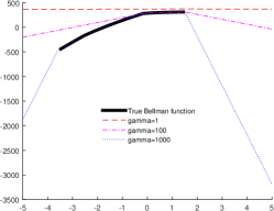
Figure 1: Graph of $V_{2}$ and of $V_{2}^{\gamma}$ for $\gamma=1,100,1000$.

Therefore, convergence of Dual SDDP with penalizations requires the coefficients $v_{tk}$ to become arbitrarily large. Proof of the following theorem is given in the Appendix.

Theorem 4.3.

Consider optimization problem (2.1) and Dual SDDP with penalizations applied to the dual of this problem. Let Assumptions (A1) and (A2) hold. Assume that samples $\xi_{t}^{\ell}$, $t=2,\ldots,T$, $\ell\geq 1$, in the forward passes are independent, that $v_{tk+1}\geq v_{tk}$ for all $t,k$, and that $\lim_{k\rightarrow+\infty}v_{tk}=+\infty$ for all stage $t$. Then the sequence $V^{k}$ is a deterministic sequence of upper bounds on the optimal value of (2.1) which converges almost surely to the optimal value of this problem.

Dual SDDP with feasibility cuts. For dual problems not satisfying the RCR assumption, a subproblem for a given stage $t$ in the forward pass can be infeasible. In this situation, as was done in Section 5 of [10] for SDDP, we can build a feasibility cut for stage $t-1$ and go back to the previous stage $t-1$ to resolve the problem with that feasibility cut added, and so on until a sequence of feasible states is obtained for all stages. In this context, no penalized slack variables are used, neither in the forward nor in the backward pass. Since the adaptations from [10] are simple, we skip the details of the derivations of this SDDP method applied to the dual. It will be tested in the numerical experiments of Section 5.

4.2 Dual SDDP for problems with uncertainty in all parameters

We have seen in Section 2.1 how to write DP equations on the dual problem of a MSLP when all data $(A_{t},B_{t},c_{t},b_{t})$ in $(\xi_{t})$ is random. In this situation, cost-to-go functions $V_{t}$ are functions $V_{t}(\pi_{t-1},\xi_{t-1})$ of both past decision $\pi_{t-1}$ and past value $\xi_{t-1}$ of process $(\xi_{t})$. Also recall that functions $V_{t}(\cdot,\xi_{t-1})$ are concave for all $\xi_{t-1}$. Therefore, Dual SDDP with penalizations from the previous section must be modified as follows. For each stage $t=2,\ldots,T,$ instead of computing just one approximation of a single function (function $V_{t}$), we now need to compute approximations of $N_{t}$ functions, namely concave cost-to-go functions $V_{t}(\cdot,\xi_{t-1j})$, $j=1,\ldots,N_{t}$. The approximation $V_{tj}^{k}$ computed for $V_{t}(\cdot,\xi_{t-1j})$ at iteration $k$ is a polyhedral function $V_{tj}^{k}$ given by:

$$V_{tj}^{k}(\pi_{t-1})=\displaystyle\min_{0\leq i\leq k}\;{\overline{\theta}}_{tj}^{i}+\langle{\overline{\beta}}_{tj}^{i},\pi_{t-1}\rangle.$$

Therefore more computational effort is needed. However, the adaptations of the method can be easily written. More specifically, at iteration $k$, in the forward pass, dual trial points are obtained replacing $V_{t}(\cdot,\xi_{t-1j})$ by $V_{tj}^{k-1}$ and in the backward pass a cut is computed at stage $t$ for $V_{t}(\cdot,\xi_{t-1j_{k}})$ with $j_{k}$ satisfying $\xi_{t-1j_{k}}=\tilde{\xi}_{t-1}^{k}$ where $\tilde{\xi}_{t-1}^{k}$ is the sampled value of $\xi_{t-1}$ at iteration $k$.

4.3 Dual SDDP for problems with interstage dependent cost coefficients

We consider problems of form (2.1) where costs $c_{t}$ affinely depend on their past while $b_{t}$ are stagewise independent. Specifically, similar to derivations of Section 3.2, suppose that $c_{t}$ follow a multiplicative vector autoregressive process of form

(4.14) $$\begin{array}[]{ll}c_{t}=\varepsilon_{t}\circ\left(\sum_{j=1}^{p}\Phi_{tj}c_{t-j}+\mu_{t}\right),\end{array}$$

with $(x\circ y)_{i}=x_{i}y_{i}$ denoting the componentwise product, and where matrices $\Phi_{tj}$ and vectors $\mu_{t}\geq 0$ as well as $c_{1},\ldots,c_{2-p}\geq 0$ are given.

We assume that the process $(b_{t},\varepsilon_{t})$ is stagewise independent and that the support of $b_{t},\varepsilon_{t}$ is the finite set

$$\{(b_{t1},\varepsilon_{t1}),\ldots,(b_{tN_{t}},\varepsilon_{tN_{t}})\},$$

with $\varepsilon_{ti}>0$ and $p_{ti}=\mathbb{P}\{(b_{t},\varepsilon_{t})=(b_{ti},\varepsilon_{ti})\}$, $i=1,\ldots,N_{t}$. For some values of $\Phi_{tj}$ (for instance for matrices with nonnegative entries), this guarantees that all realizations of the price process $\{c_{t}\}$ are positive. The developments which follow can be easily extended to other linear models for $\{c_{t}\}$, for instance SARIMA or PAR models, see [9] for the definition of state vectors of minimal size for generalized linear models.

Using the notation $c_{t_{1}:t_{2}}=(c_{t_{1}},c_{t_{1}+1},\ldots,c_{t_{2}-1},c_{t_{2}})$ for $t_{1}\leq t_{2}$ integer, for the corresponding primal problem (of the form (2.1)), we can write the following Dynamic Programming equations: define $\mathcal{Q}_{T+1}\equiv 0$ and for $t=2,\ldots,T$,

(4.15) $$\mathcal{Q}_{t}(x_{t-1},c_{t-p:t-1})=\mathbb{E}_{b_{t},\varepsilon_{t}}\Big{[}Q_{t}(x_{t-1},c_{t-p:t-1},b_{t},\varepsilon_{t})\Big{]}$$

where $Q_{t}(x_{t-1},c_{t-p:t-1},b_{t},\varepsilon_{t})$ is given by

(4.16) $$\begin{array}[]{ll}\displaystyle\min_{x_{t}\geq 0}\Big{[}\varepsilon_{t}\circ\Big{(}\displaystyle\sum_{j=1}^{p}\Phi_{tj}c_{t-j}+\mu_{t}\Big{)}\Big{]}^{\top}x_{t}+\mathcal{Q}_{t+1}\Big{(}x_{t},c_{t+1-p:t-1},\varepsilon_{t}\circ\Big{(}\displaystyle\sum_{j=1}^{p}\Phi_{tj}c_{t-j}+\mu_{t}\Big{)}\Big{)}\\ A_{t}x_{t}+B_{t}x_{t-1}=b_{t},\end{array}$$

while the first stage problem is

$$\begin{array}[]{l}\displaystyle\min_{x_{1}\geq 0}\;c_{1}^{\top}x_{1}+\mathcal{Q}_{2}(x_{1},c_{2-p:1})\\ A_{1}x_{1}=b_{1}.\end{array}$$

Standard SDDP does not apply directly to solve Dynamic Programming equations (4.15)-(4.16) because functions $\mathcal{Q}_{t}$ given by (4.15)-(4.16) are not convex. Nevertheless, we can use the Markov Chain discretization variant of SDDP to solve Dynamic Programming equations (4.15)-(4.16). On the other hand, as pointed above, it is possible to apply SDDP for the dual problem with the added state variables. Along the lines of Section 2.1 we can write Dynamic Programming equations for the dual, now with function $V_{t}$ depending on $\pi_{t-1},c_{t-1},\ldots,c_{t-p}$.

These functions are concave and therefore we can apply Dual SDDP with penalizations to these DP equations to build polyhedral approximations of these functions $V_{t}$ of form

(4.17) $$V_{t}^{k}(\pi_{t-1},c_{t-1},\ldots,c_{t-p})=\min_{0\leq i\leq k}\theta_{t}^{i}+\langle\beta_{t0}^{i},\pi_{t-1}\rangle+\sum_{j=1}^{p}\langle\beta_{tj}^{i},c_{t-j}\rangle$$

at iteration $k$.

5 Numerical experiments

In this section, we report numerical results obtained applying Primal SDDP and variants of Dual SDDP to the inventory problem and to the Brazilian interconnected power system problem. All methods were implemented in Matlab and run on an Intel Core i7, 1.8GHz, processor with 12,0 Go of RAM. Optimization problems were solved using Mosek [1].

5.1 Dual SDDP for the inventory problem

We consider the inventory problem (3.3) with parameters $a_{t}=1.5+\cos(\frac{\pi t}{6})$, $p_{ti}=\frac{1}{N}$ where $N$ is the number of realizations for each stage, $\xi_{tj}=(5+0.5t)(1.5+0.1z_{tj})$ where $(z_{t1},\ldots,z_{tN})$ is a sample from the standard Gaussian distribution, $x_{0}=10$, $g_{t}=2.8$, and $h_{t}=0.2$.

Illustrating the correctness of DP equations (2.5), (2.6), (2.7) and checking the convergence of the variants of Dual SDDP.

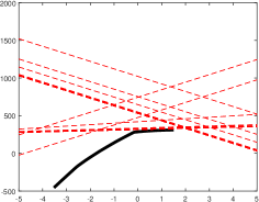
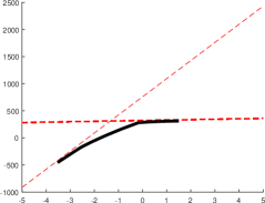
Figure 2: Graph of $V_{2}$ (bold black solid line) and cuts computed for $V_{2}$ by Dual SDDP with penalizations $v_{tk}=100$ (left panel) and Dual SDDP with feasibility cuts (right panel).

We solve this inventory problem using Dynamic Programming applied both to DP equations (2.5), (2.6), (2.7) and to DP equations (4.11)-(4.12) for $\gamma=1,10,1000$. In this latter case, we obtain approximations of functions $V_{t}^{\gamma}$. We also run Primal SDDP, Dual SDDP with feasibility cuts, and Dual SDDP with penalties $v_{tk}=1$, $10$, $1000$, on the same instance, knowing that Dual SDDP variants were run for 100 iterations (the upper bounds computed by these methods stabilize in less than 10 iterations) and Primal SDDP was stopped when the gap is $<0.1$ where the gap is defined as $\frac{Ub-Lb}{Ub}$ where $Ub$ and $Lb$ correspond to upper and lower bounds computed by Primal SDDP along iterations. The lower bound $Lb$ is the optimal value of the first stage problem and the upper bound $Ub$ is the upper end of a 97.5%-one-sided confidence interval on the optimal value obtained using the sample of total costs computed by all previous forward passes. With this stopping criterion and the considered instance of the inventory problem, Primal SDDP was run for 232 iterations.

In Figure 2, we report the graph of $V_{2}$ and the cuts computed for $V_{2}$ by Dual SDDP with feasibility cuts (right panel) and Dual SDDP with penalties $v_{tk}=100$ (left panel). All cuts are, as expected, upper bounding affine functions for $V_{2}$ on its domain. However, it is interesting to notice that for Dual SDDP with feasibility cuts, few different cuts are computed and these cuts are tangent or very close to $V_{2}$ at the trial points. On the contrary, Dual SDDP with penalties may compute many cuts dominated by others on the domain of $V_{2}$. Therefore, cut selection techniques, for instance along the lines of [11] [13] using Limited Memory Level 1 cut selection, could be useful for Dual SDDP.

We report in Table 1 the approximate optimal values and the time needed to compute them with Primal SDDP, Dual SDDP, and Dynamic Programming applied to respectively (2.5), (2.6), (2.7) and (4.11), (4.12), (4.13) with $\gamma=1,100,1000$. The approximate optimal values reported are the last upper bound computed for variants of Dual SDDP and the last lower bound computed for Primal SDDP. All approximate optimal values are very close (showing that all variants were correctly implemented) and Dynamic Programming is much slower than the other sampling-based algorithms. For Dual SDDP with penalization, if penalties are too small the upper bound can be $+\infty$ while if penalties are sufficiently large the algorithm converges to an optimal policy.

Method	Optimal value	CPU time (s.)
DP on (2.5), (2.6), (2.7)	321.6	685
DP on (4.11), (4.12), (4.13), $\gamma=1$	$+\infty$	2 860
DP on (4.11), (4.12), (4.13), $\gamma=100$	322.2	3 808
DP on (4.11), (4.12), (4.13), $\gamma=1000$	321.8	3 376
Primal SDDP	322.5	105
Dual SDDP with penalties, $v_{tk}=1$	2 131.4	9.4
Dual SDDP with penalties, $v_{tk}=100$	322.5	11.3
Dual SDDP with penalties, $v_{tk}=1000$	322.5	11.9
Dual SDDP with feasibility cuts	322.5	10.6

Table 1: Optimal value and CPU time needed (in seconds) to compute them on an instance of the inventory problem with $T=N_{t}=20$ by Dynamic Programming (DP), Primal SDDP, and variants of Dual SDDP.

Finally, we report for this instance in Figure 3 the evolution of the lower bound $Lb$ and upper bound $Ub$ computed by Primal SDDP and the upper bounds computed by Dual SDDP with penalties $v_{tk}=1000$ and Dual SDDP with feasibility cuts. With Dual SDDP, the upper bound is naturally large at the first iteration but decreases much quicker than the upper bound $Ub$ computed by Primal SDDP, especially for Dual SDDP with feasibility cuts, with all upper bounds converging to the optimal value of the problem.

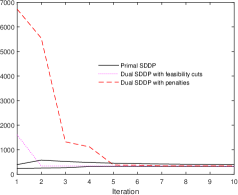
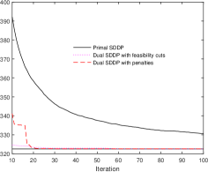
Figure 3: Left: upper and lower bounds computed by Primal SDDP and upper bounds computed by Dual SDDP with feasibility cuts and Dual SDDP with penalties $v_{tk}=1000$ for the first 10 iterations. Right: same outputs for iterations 10,$\ldots,100$.

Tests on a larger instance. We now run Primal and Dual SDDP on a larger instance with $T=100$ and $N_{t}=100$ for 600 iterations. The evolution of the upper bounds computed along the iterations of Dual SDDP (both with feasibility cuts and with penalizations $v_{tk}=1000$) and of the upper and lower bounds computed by Primal SDDP are reported in Table 2 for iterations $2,3,5,10,50,100,200,300,400,500,$ and $600$. We see that for the first iterations, the upper bound decreases more quickly with the variants of Dual SDDP, the most important decrease being obtained for Dual SDDP with feasibility cuts. However, on this instance, the convergence of Dual SDDP with feasibility cuts is slower, i.e., a solution of high accuracy is obtained quicker using Dual SDDP with penalizations. More precisely, we fix confidence levels $\varepsilon=0.2,0.15,0.1,0.05,0.01$, and for each confidence level, we compute the time needed, running Primal and Dual SDDP in parallel, to obtain a solution with relative accuracy $\varepsilon$ stopping the algorithm when the upper bound Ub_D computed by a variant of Dual SDDP and the lower bound Lb, computed by Primal SDDP, satisfies (Ub_D-Lb)/Ub_D$<\varepsilon$. The results are reported in Table 3. In this table, we also report the time needed to obtain a solution of relative accuracy $\varepsilon$ using only the information provided by Primal SDDP, stopping the algorithm when (Ub-Lb)/Ub$<\varepsilon$.

We observe that if $\varepsilon$ is not too small, the smallest CPU time is obtained combining Primal SDDP with Dual SDDP with feasibility cuts while when $\varepsilon$ is small (0.05 and 0.01) the smallest CPU time is obtained combining Primal SDDP with Dual SDDP with penalizations. For $\varepsilon=0.05$ and $0.01$, 600 iterations are even not enough to get a solution of relative accuracy $\varepsilon$ using Primal SDDP or combining Primal SDDP and Dual SDDP with feasibility cuts.

Iteration	Primal SDDP Lb	Primal SDDP Ub	Dual SDDP with feasibility cuts	Dual SDDP with penalties
2	656.4	25 443	20 002	20 015
3	713.1	19 340	8 693.1	20 012
5	3361.8	14 800	7 246.8	19 993
10	5330.1	10 662	5 736.6	16 452
50	5483.1	6 594.5	5721.8	5500.9
100	5483.5	6 039.2	5715.1	5484.8
200	5483.6	5 762.4	5710.0	5484.2
300	5483.7	5 671.0	5704.6	5484.0
400	5483.7	5 625.3	5702.7	5483.9
500	5483.7	5 597.9	5702.5	5483.8
600	5483.7	5 579.9	5702.2	5483.8

Table 2: For an instance of the inventory problem with $T=N_{t}=100$, lower bound Lb and upper bound Ub computed by Primal SDDP and upper bounds computed by Dual SDDP with feasibility cuts and Dual SDDP with penalties $v_{tk}=1000$ along iterations.

In Figure 4, we report the cumulative CPU time along iterations of all methods. We see that each iteration requires a similar computational bulk and the CPU time increases exponentially with the number of iterations.

$\varepsilon$	Primal SDDP	Dual SDDP with feasibility cuts	Dual SDDP with penalties $v_{tk}=1000$
0.2	300.2	29.5	35.8
0.15	459.8	35.8	41.2
0.1	825.6	48.3	48.3
0.05	2366.2	96.1	61.5
0.01	-	-	103.2

Table 3: Time needed (in seconds) to obtain a solution of relative accuracy $\varepsilon$ with Primal SDDP, Dual SDDP with feasibility cuts, and Dual SDDP with penalties $v_{tk}=1000$ for an instance of the inventory problem with $T=N_{t}=100$.

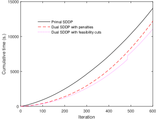
Figure 4: Cumulative CPU time along iterations of Primal SDDP, Dual SDDP with feasibility cuts, and Dual SDDP with penalizations $v_{tk}=1000$.

5.2 Sensitivity analysis for the inventory problem

Consider the inventory problem of Section 5.1 with $(\mathcal{D}_{t})$ as in (3.4) and $T=10$ stages. For this problem, the derivatives from Proposition 3.1 are given by

(5.1) $$\partial\vartheta(\phi,\mu)/\partial\phi=\partial L(\bar{x},\bar{y},\bar{\pi})/\partial\phi={\mathbb{E}}\left[\sum_{t=1}^{T}\bar{\pi}_{t}\epsilon_{t}\mathcal{D}_{t-1}\right],$$

(5.2) $$\partial\vartheta(\phi,\mu)/\partial\mu=\partial L(\bar{x},\bar{y},\bar{\pi})/\partial\mu={\mathbb{E}}\left[\sum_{t=1}^{T}\bar{\pi}_{t}\epsilon_{t}\right],$$

where $(\bar{x},\bar{y})$ is an optimal solution of the primal problem and $\bar{\pi}$ are the corresponding Lagrange multipliers. Our goal is to compute these derivatives solving the primal and dual problems by respectively Primal and Dual SDDP.

We consider $4$ instances with $(\phi,\mu)=(0.01,0.1)$, $(0.01,3.0)$, $(0.001,0.1)$, and $(0.001,3.0)$. The remaining parameters of these instances are those from the previous section. We discretize both the primal and dual problem into $N_{t}=100$ samples for each stage $t=2,\ldots,10$. We take the relative error $\varepsilon=0.01$ for the stopping criterion and use $10\,000$ Monte Carlo simulations to estimate the expectations in (5.1), (5.2). For Primal SDDP, the upper bound Ub and lower bound Lb at termination are given in Table 4 for the four instances.

Bound	Instance 1	Instance 2	Instance 3	Instance 4
Ub	17.9176	478.687	15.3940	404.242
Lb	17.9163	475.017	15.3927	402.913

Table 4: Upper and lower bounds at the last iteration of Primal SDDP.

The optimal mean values of Lagrangian multipliers for the demand constraints computed, for a given stage $t\geq 2$, averaging over the $10\,000$ values obtained simulating $10\,000$ forward passes after termination, are given in Table 5. In this table, LM stands for the multipliers obtained using Primal SDDP as explained in Remark 2.3 whereas Dual stands for the multipliers obtained using Dual SDDP with penalties. The fact that the multipliers obtained are close for both methods illustrates the validity of the two alternatives we discussed in Sections 3-4 to compute derivatives of the value function of a MSP.

Stage	Instance 1		Instance 2		Instance 3		Instance 4
	LM	Dual	LM	Dual	LM	Dual	LM	Dual
2	0.2465	0.2373	1.6701	1.66959	0.0444	0.0328	1.666	1.666
3	0.3218	0.31095	1.4098	1.4120	0.1421	0.1340	1.406	1.409
4	0.3268	0.3221	0.9862	0.9861	0.19439	0.18974	0.984	0.984
5	0.3086	0.3058	0.6330	0.6329	0.2145	0.2128	0.6327	0.6327
6	0.3408	0.3412	0.49998	0.499897	0.2708	0.2717	0.4999	0.4998
7	0.5026	0.5051	0.63397	0.63397	0.4378	0.4418	0.6339	0.6339
8	0.7047	0.7049	0.8348	0.8340	0.6404	0.6413	0.8349	0.8334
9	0.8985	0.9032	1.0322	1.0343	0.83501	0.8401	1.0315	1.0343
10	1.1022	1.1037	1.2302	1.2365	1.03926	1.04091	1.23	1.23

Table 5: Comparison between optimal Lagrange multipliers from Primal SDDP and Dual SDDP with penalties.

With optimal dual solutions $\{\bar{\pi}_{t}\}$ and the realizations of $\{D_{t}\}$ and $\{\epsilon_{t}\}$ at hand, we are able to compute the sensitivity of the optimal value with respect to $\phi$ and $\mu$, using (5.1) and (5.2), with expectations estimated for $10\,000$ Monte Carlo simulations. We benchmark our method against the finite-difference method. Specifically, for value function $\vartheta$, the finite-difference method approximates the derivative with respect to $u_{0}$ by $v^{\prime}(u_{0})\approx\frac{v(u_{0}+\delta)-v(u_{0}-\delta)}{2\delta}$ for some small $\delta$.

The sensitivity of the optimal value of the inventory problem with respect to $(\phi,\mu)$ is displayed in Table 6. In this table, S-$\phi$ and S-$\mu$ denote the derivatives with respect to $\phi$ and $\mu$ computed by our method, and fd-$\phi$, fd-$\mu$ denote the derivatives computed by the finite-difference method. In order to measure the difference between the two methods, we also compute S-gap-$\phi$ and S-gap-$\mu$, where S-gap-$\phi:=\frac{|\text{fd-}\phi-\text{S-}\phi|}{|\text{fd-}\phi|}\times 100\%$ and S-gap-$\mu:=\frac{|\text{fd-}\mu-\text{S-}\mu|}{|\text{fd-}\mu|}\times 100\%$.

Instance	fd-$\phi$	S-$\phi$	S-gap-$\phi$($\%$)	fd-$\mu$	S-$\mu$	S-gap-$\mu$($\%$)
1	403.604	401.094	0.622	164.578	164.158	0.255
2	10 716.111	10 671.262	0.419	185.346	184.847	0.270
3	269.514	269.443	0.026	134.646	134.463	0.136
4	7 780.570	7 770.274	0.132	158.017	158.001	0.0101

Table 6: Sensitivity of the optimal value with respect to $\phi$ and $\mu$ by the two methods.

We observe that the derivatives obtained by both methods are close to each other, especially when $\phi$ and $\mu$ are small. This is because small $\phi$ and $\mu$ gives rise to less variability in the demand. Note also that the finite-difference method is more time consuming since it requires computing the optimal value twice. Instead, our method only needs to solve the model once. Moreover, computing the Lagrange multipliers does not significantly consume CPU time, as they are generated as a by-product of Primal SDDP. Alternatively, as discussed above, one can compute the optimal multipliers using Dual SDDP with penalties. Another drawback of the finite-difference method lies in its numerical instability. Indeed, the method is more accurate when $\delta$ is very small. However, the division by a very small number generates bias while our approach is more stable.

5.3 Dual SDDP for an hydro-thermal generation problem

We repeat the experiments of Section 5.1 for the Brazilian interconnected power system problem discussed in [7] for $T=12$ stages and $N_{t}=50$ inflow realizations for every stage. These realizations are obtained calibrating log-normal distributions for each month of the year using historical data of inflows and sampling from these distributions. The data used for these simulations (including the inflow scenarios) is available on Github.

We solve this problem using Primal SDDP and Dual SDDP with penalizations. For this variant of Dual SDDP, a general procedure to define sequences of penalizations $(v_{tk})$ ensuring convergence of the corresponding Dual SDDP method is to take $v_{tk}=\gamma_{0}\alpha^{k-1}{\textbf{e}}$, $k\geq 1$, $t=2,\ldots,T$, with $\alpha>1$, $\gamma_{0}>0$. For numerical reasons, we also take a large upper bound $U$ for these sequences and use

(5.3) $$v_{tk}=\min(U,\gamma_{0}\alpha^{k-1}){\textbf{e}},\;k\geq 1,t=2,\ldots,T.$$

We consider three variants of Dual SDDP: for the first variant, denoted by Dual SDDP 1, $v_{tk}$ are as in (5.3) with $\gamma_{0}=10^{4}$, $\alpha=1.3$, $U=10^{10}$. To illustrate the fact that for constant sequences $v_{tk}=\gamma_{0}$, Dual SDDP converges (resp. does not converge) for sufficiently large constants $\gamma_{0}$ (resp. sufficiently small constants $\gamma_{0}$) we also define two other variants corresponding to $U=+\infty$, $\gamma_{0}=10^{9}$, $\alpha=1$, and $U=+\infty$, $\gamma_{0}=10^{6}$, $\alpha=1$, in (5.3), respectively denoted by Dual SDDP 2 and Dual SDDP 3.

We run Dual SDDP for 1000 iterations and Primal SDDP for 3000 iterations. The evolution of the upper and lower bounds computed by the methods for the first 1000 iterations is given in Figure 5.

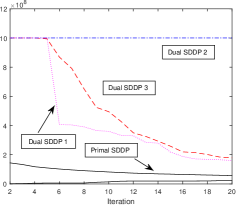
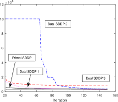
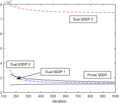
Figure 5: Top left: upper and lower bounds computed by Primal SDDP and upper bounds computed by Dual SDDP 1, Dual SDDP 2, and Dual SDDP 3, for the first 20 iterations for an instance of the hydro-thermal problem with $T=12$, $N_{t}=50$. Top right: same outputs for iterations 21,$\ldots,150$. Bottom: same outputs for iterations 151,$\ldots,1000$.

More precisely, the values of these bounds for iterations 2, 5, 10, 50, 100, 150, 200, 250, 300, 350, 400, 1000, and 3000 are reported in Table 7. We observe that parameter $\gamma_{0}$ for Dual SDDP 3 is too small to allow this method to converge to the optimal value of the problem whereas the other two variants Dual SDDP 1 and Dual SDDP 2 of Dual SDDP converge. Naturally, these methods start with large upper bounds but after a few tens of iterations the upper bounds with Dual SDDP 1 and Dual SDDP 2 are better than the upper bound computed by Primal SDDP. In particular, it is interesting to notice that the best (lowest) upper bounds are obtained with the variant of Dual SDDP that uses adaptive penalizations, i.e., penalizations that increase with the number of iterations before reaching value $U$ in (5.3).

Iteration	Primal SDDP Lb	Primal SDDP Ub	Dual SDDP 1	Dual SDDP 2	Dual SDDP 3
2	$1.317$	$143.98$	$1000.2$	$1000.2$	$1000.2$
5	$5.5588$	$109.36$	$1000.2$	$1000.2$	$994.04$
10	$14.032$	$81.728$	$360.40$	$1000.2$	$495.08$
50	$23.670$	$41.346$	$54.999$	$1000.2$	$96.720$
100	$24.787$	$35.502$	$36.322$	$64.072$	$82.494$
150	$25.111$	$32.447$	$30.685$	$35.595$	$79.465$
200	$25.249$	$30.672$	$29.076$	$30.404$	$78.059$
250	$25.374$	$30.079$	$28.215$	$28.943$	$76.917$
300	$25.436$	$29.434$	$27.710$	$28.030$	$76.344$
350	$25.477$	$29.014$	$27.309$	$27.532$	$75.852$
400	$25.526$	$28.626$	$27.110$	$27.188$	$75.526$
1000	$25.703$	$27.175$	$26.304$	$26.335$	$74.292$
3000	$25.798$	$26.883$	-	-

Table 7: For an instance of the hydro-thermal problem with $T=12$, $N_{t}=50$, lower bound Lb and upper bound Ub computed by Primal SDDP and upper bounds computed by variants of Dual SDDP along iterations. All costs have been divided by $10^{6}$ to improve readability.

We also report in Table 8 the relative error $\frac{{\tt{Upper}}_{M}(i)-{\tt{Lower}}_{{\tt{SDDP}}}(i)}{{\tt{Upper}}_{M}(i)}$ for iterations $i=100$, $200$, $300$, $400$, $500$, $800$, and $1000$ for all methods M where ${\tt{Upper}}_{M}(i)$ and ${\tt{Lower}}_{{\tt{SDDP}}}(i)$ are respectively the upper bound computed by method M at iteration $i$ and the lower bound computed by Primal SDDP at iteration $i$. For iterations 300 on, the relative error is much smaller with variants of Dual SDDP, meaning that Primal SDDP overestimates the optimality gap.

Iteration	Primal SDDP	Dual SDDP 1	Dual SDDP 2
100	0.30	0.32	0.61
200	0.18	0.13	0.17
300	0.14	0.08	0.09
400	0.11	0.06	0.06
500	0.09	0.05	0.05
800	0.07	0.03	0.03
1000	0.05	0.02	0.02

Table 8: Relative error as a function of the number of iterations for Primal SDDP, Dual SDDP 1, and Dual SDDP 2.

However, each iteration of Dual SDDP takes more time as can be seen in Figure 6 which reports the cumulative CPU time for all methods. More precisely, running Dual and Primal SDDP in parallel, we can compute the time needed to obtain a solution of relative accuracy $\varepsilon$ using the standard stopping criterion for Primal SDDP (see [27]) or using the lower bound from Primal SDDP and the upper bound from Dual SDDP, and computing the relative error obtained with these bounds each time a new bound (either lower bound or upper bound) is computed. The results are reported in Table 9. We see that due to the fact that Dual SDDP iterations are more time consuming, for all relative accuracies but one, the use of the stopping criterion based on Dual SDDP upper bounds requires more computational bulk. From this experiment, performed on a larger problem (in terms of size of the state vector and number of control variables for each stage) than the inventory problem of Section 5.1, it seems that the use of Dual SDDP for a stopping criterion of Primal SDDP will decrease the overall computational bulk only for small problems (having a limited to small number of controls, state variables, and scenarios).

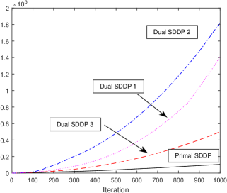
Figure 6: Cumulative CPU time for Primal SDDP, Dual SDDP 1, Dual SDDP 2, and Dual SDDP 3.

$\varepsilon$	Primal SDDP	Dual SDDP 1	Dual SDDP 2
0.3	515	1 042	4 133
0.2	1 167	1 895	7 446
0.15	1 659	2 910	9 882
0.1	3 168	5 114	16 387
0.075	5 359	8 003	22 457
0.05	11 124	15 738	35 113
0.04	45 391	23 449	51 381

Table 9: Time (in seconds) needed to obtain a solution of relative accuracy $\varepsilon$ with Primal SDDP and variants of Dual SDDP for an instance of the hydro-thermal problem.

6 Appendix

In this Appendix, we prove Lemma 4.1, Proposition 4.2, and Theorem 4.3.

We first need more notation. We introduce the sequence of functions

(6.1) $${\overline{V}}_{T}^{k}(\pi_{T-1}):=\begin{array}[]{l}\max\limits_{\pi_{T1},\ldots,\pi_{TN_{T}},\zeta_{T}}\;\displaystyle\sum\limits_{j=1}^{N_{T}}p_{Tj}b_{Tj}^{\top}\pi_{Tj}-v_{Tk}^{\top}\zeta_{T}\\ A_{T}^{\top}\pi_{Tj}\leq c_{T},\;j=1,\ldots,N_{T},\\ A_{T-1}^{\top}\pi_{T-1}+\displaystyle\sum_{j=1}^{N_{T}}p_{Tj}B_{Tj}^{\top}\pi_{Tj}\leq c_{T-1}+\zeta_{T},\\ \zeta_{T}\geq 0,{\underline{\pi}}_{T}\leq\pi_{Tj}\leq{\overline{\pi}}_{T},\;j=1,\ldots,N_{T},\end{array}$$

and for $t=2,\ldots,T-1$, the sequence of functions

(6.2) $${\overline{V}}_{t}^{k}(\pi_{t-1}):=\begin{array}[]{l}\max\limits_{\pi_{t1},\ldots,\pi_{tN_{t}},\zeta_{t}}\;\displaystyle\sum\limits_{j=1}^{N_{t}}p_{tj}\left(b_{tj}^{\top}\pi_{tj}+{V}_{t+1}^{k}(\pi_{tj})\right)-v_{tk}^{\top}\zeta_{t}\\ A_{t-1}^{\top}\pi_{t-1}+\displaystyle\sum_{j=1}^{N_{t}}p_{tj}B_{tj}^{\top}\pi_{tj}\leq c_{t-1}+\zeta_{t},\\ \zeta_{t}\geq 0,{\underline{\pi}}_{t}\leq\pi_{tj}\leq{\overline{\pi}}_{t},\;j=1,...,N_{t}.\\ \end{array}$$

Due to Assumption (A1) we can represent the scenarios for $\xi_{1},\xi_{2},\ldots,\xi_{T}$, by a scenario tree of depth $T+1$ where the root node $n_{0}$ associated to a stage $0$ (with decision $x_{0}$ taken at that node) has one child node $n_{1}$ associated to the first stage. We denote by $\mathcal{N}$ the set of nodes and for a node $n$ of the tree, by $(x_{n},\pi_{n})$ a primal-dual pair at that node and by $\xi_{n}$ the realization of process $(\xi_{t})$ at node $n$ (this realization $\xi_{n}$ contains in particular the realizations $c_{n}$ of $c_{t}$, $b_{n}$ of $b_{t}$, $A_{n}$ of $A_{t}$, and $B_{n}$ of $B_{t}$).

Proof of Lemma 4.1. Let $1\leq t\leq T$ and let us fix a node $m$ of stage $t$. Let $\overline{A}_{m}$ such that constraints $A_{m}x_{m}+B_{m}x_{F(m)}=b_{m}$ are rewritten in compact form $\overline{A}_{m}x=b_{m}$ in terms of vector $x=(x_{n})_{n\in\mathcal{N}}$ of decision variables in the scenario tree. The dual function obtained dualizing the coupling constraints of node $m$ is given by

$$\theta(\pi_{m})=\begin{array}[]{l}\min\;\mathbb{E}[c^{\top}x]+\pi_{m}^{\top}(A_{m}x_{m}+B_{m}x_{F(m)}-b_{m})\\ x\in\mathcal{S}_{m},\end{array}$$

for $\mathcal{S}_{m}=\{x=(x_{n})_{n\in\mathcal{N}}:x\geq 0\}\cap\mathcal{A}_{m}$ where $\mathcal{A}_{m}=\{x=(x_{n})_{n\in\mathcal{N}}:A_{n}x_{n}+B_{n}x_{F(n)}=b_{n},\forall n\neq m,n\in\mathcal{N}\}.$

By Linear Programming Duality, the optimal value $\mathcal{Q}_{1}(x_{0})$ of primal problem (2.1) is the optimal value of the dual problem

(6.3) $$\max\{\theta(\pi_{m}):\pi_{m}\in\mathbb{R}^{m_{t}}\}$$

which can clearly be written as

(6.4) $$\mathcal{Q}_{1}(x_{0})=\max_{\pi_{m}}\{\theta(\pi_{m}):\pi_{m}={\overline{A}}_{m}x-{b}_{m},x\in\mbox{Aff}(\mathcal{S}_{m})\},$$

where $\mbox{Aff}(\mathcal{S}_{m})$ is the affine hull of $\mathcal{S}_{m}$. We now bound the optimal solutions of dual problem (6.4). Since (6.3) and (6.4) have the same optimal values, adding these bounds as constraints on $\pi_{m}$ in (6.3) does not change its optimal value. Since $\hat{x}>0$ there is $r>0$ such that

(6.5) $$\mathbb{B}(\hat{x},r)\subseteq\{x\geq 0\}.$$

We argue that $\mbox{Aff}(\mathcal{S}_{m})=\mathcal{A}_{m}$. Indeed, the inclusion $\mbox{Aff}(\mathcal{S}_{m})\subseteq\mathcal{A}_{m}$ is clear. Now if $x\in\mathcal{A}_{m}$ then if $x=\hat{x}$ we have that $x\in\mathcal{S}_{m}\subseteq\mbox{Aff}(\mathcal{S}_{m})$ and if $x\neq\hat{x}$, recalling that $\hat{x}\in\mathcal{A}_{m}$ satisfies (6.5) we have that

$$y:=\hat{x}+\frac{r}{2}\frac{x-\hat{x}}{\|x-\hat{x}\|}\in\mathcal{A}_{m}\cap\mathbb{B}(\hat{x},r)\subseteq\mathcal{S}_{m}.$$

Therefore $x$ belongs to the line that contains $y$ and $\hat{x}$ with $y,\hat{x}$ belonging to $\mathcal{S}_{m}$ which implies $x\in\mbox{Aff}(\mathcal{S}_{m})$ and $\mbox{Aff}(\mathcal{S}_{m})=\mathcal{A}_{m}$.

It follows that

$$\mathbb{B}(\hat{x},r)\cap\mbox{Aff}(\mathcal{S}_{m})=\mathbb{B}(\hat{x},r)\cap\mathcal{A}_{m}\subseteq\mathcal{S}_{m}$$

and that there is $\rho_{*}(m)>0$ such that

$$\mathbb{B}(0,\rho_{*})\cap(\overline{A}_{m}\mathcal{A}_{m}-b_{m})\subseteq\overline{A}_{m}(\mathbb{B}(\hat{x},r)\cap\mathcal{A}_{m})-b_{m}.$$

Let $\bar{\pi}_{m}$ be an optimal solution of problem (6.4) and let $z=0$ if $\bar{\pi}_{m}=0$ and $z=-\frac{\bar{\pi}_{m}}{\|\bar{\pi}_{m}\|_{2}}\rho_{*}$ otherwise. Observe that $z\in\mathbb{B}(0,\rho_{*})\cap(\overline{A}_{m}\mathcal{A}_{m}-b_{m})$ and therefore $z\in\overline{A}_{m}(\mathbb{B}(\hat{x},r)\cap\mathcal{A}_{m})-b_{m}\subseteq\overline{A}_{m}\mathcal{S}_{m}-b_{m}$ and $z$ can be written $z={\overline{A}}_{m}\tilde{x}-b_{m}$ for $\tilde{x}\in\mathbb{B}(\hat{x},r)\cap\mathcal{S}_{m}$. It follows that

$$\begin{array}[]{lcl}\mathcal{Q}_{1}(x_{0})=\theta(\bar{\pi}_{m})&\leq&\mathbb{E}[c^{\top}\tilde{x}]+\bar{\pi}_{m}^{\top}({\overline{A}}_{m}\tilde{x}-b_{m})\\ &\leq&\mathbb{E}[c^{\top}\hat{x}]+r\sum_{t=1}^{T}\mathbb{E}[\|c_{t}\|_{2}]+\bar{\pi}_{m}^{\top}z\\ &=&\mathbb{E}[c^{\top}\hat{x}]+r\sum_{t=1}^{T}\mathbb{E}[\|c_{t}\|_{2}]-\rho_{*}(m)\|\bar{\pi}_{m}\|_{2}\end{array}$$

which gives for every node $n$ of stage $t$ that

$$\|\bar{\pi}_{n}\|_{2}\leq\max_{m\in{\tt{Nodes}}(t)}\frac{\mathbb{E}[c^{\top}\hat{x}]-\mathcal{Q}_{1}(x_{0})+r\sum_{t=1}^{T}\mathbb{E}[\|c_{t}\|_{2}]}{\rho_{*}(m)}$$

with corresponding box constraints $\underline{\pi}_{t},\overline{\pi}_{t}$ where ${\tt{Nodes}}(t)$ are the nodes of stage $t$. $\hfill\square$

Proof of Proposition 4.2. We show by induction on $k$ that $V_{t}\leq{V}_{t}^{k}$ for $t=2,\ldots,T$. For $k=0$ these relations hold by definition. Assume that for some $k\geq 1$ we have $V_{t}\leq{V}_{t}^{k-1}$ for $t=2,\ldots,T$. We show by backward induction on $t$ that $V_{t}\leq{V}_{t}^{k}$ for $t=2,\ldots,T$. Observe that for any $\pi_{T-1}$, optimization problem (6.1) with optimal value ${\overline{V}}_{T}^{k}(\pi_{T-1})$ is feasible. Indeed, since primal problem (2.1) is feasible and has a finite optimal value, the corresponding dual problem is feasible which implies that there is $\pi_{T1},\ldots,\pi_{TN_{T}}$ satisfying $A_{T}^{\top}\pi_{Tj}\leq c_{T}$, ${\underline{\pi}}_{T}\leq\pi_{Tj}\leq{\overline{\pi}}_{T}$, $j=1,\ldots,N_{T}$, and for every such points we can find $\zeta_{T}\geq 0$ satisfying the remaining constraints in (6.1). Therefore ${\overline{V}}_{T}^{k}(\pi_{T-1})$ is finite for every $\pi_{T-1}$ and is the optimal value of the corresponding dual optimization problem, i.e., for any $\pi_{T-1}$ we get

$${\overline{V}}_{T}^{k}(\pi_{T-1})=\begin{array}[]{l}\displaystyle\min_{\alpha,\delta,{\overline{\Psi}},{\underline{\Psi}}}\;\delta^{\top}(c_{T-1}-A_{T-1}^{\top}\pi_{T-1})+c_{T}^{\top}\sum_{j=1}^{N_{T}}\alpha_{j}+\sum_{j=1}^{N_{T}}{\overline{\Psi}}_{j}^{\top}{\overline{\pi}}_{T}-\sum_{j=1}^{N_{T}}{\underline{\Psi}}_{j}^{\top}{\underline{\pi}}_{T}\\ A_{T}\alpha_{j}+p_{Tj}B_{Tj}\delta-{\underline{\Psi}}_{j}+{\overline{\Psi}}_{j}=p_{Tj}b_{Tj},\;j=1,\ldots,N_{T},\\ 0\leq\delta\leq v_{Tk},\alpha_{j},{\underline{\Psi}}_{j},{\overline{\Psi}}_{j}\geq 0,\;j=1,\ldots,N_{T}.\end{array}$$

Using this dual representation and the definition of $\overline{\theta}_{T}^{k},{\overline{\beta}}_{T}^{k}$, we get for every $\pi_{T-1}$:

(6.6) $$\overline{\theta}_{T}^{k}+\langle{\overline{\beta}}_{T}^{k},\pi_{T-1}\rangle\geq{\overline{V}}_{T}^{k}(\pi_{T-1}).$$

Recalling representation (6.1) for ${\overline{V}}_{T}^{k}(\pi_{T-1})$, observe that for every $\pi_{T-1}\in\mbox{dom}(V_{T})$ we have ${\overline{V}}_{T}^{k}(\pi_{T-1})\geq V_{T}(\pi_{T-1})$ whereas for $\pi_{T-1}\notin\mbox{dom}(V_{T})$ we have $V_{T}(\pi_{T-1})=-\infty$ while ${\overline{V}}_{T}^{k}(\pi_{T-1})$ is finite, which shows that for every $\pi_{T-1}$ we have ${\overline{V}}_{T}^{k}(\pi_{T-1})\geq V_{T}(\pi_{T-1})$, which, combined with (6.6) and the induction hypothesis, gives

$$V_{T}^{k}(\pi_{T-1})\geq V_{T}(\pi_{T-1})$$

for every$\pi_{T-1}$.

Now assume that $V_{t+1}^{k}(\pi_{t})\geq V_{t+1}(\pi_{t})$ for all $\pi_{t}$ for some $t\in\{2,\ldots,T-1\}$. We want to show that $V_{t}^{k}(\pi_{t-1})\geq V_{t}(\pi_{t-1})$ for all $\pi_{t-1}$. First observe that for every $\pi_{t-1}$, linear program (6.2) with optimal value ${\overline{V}}_{t}^{k}(\pi_{t-1})$ is feasible and has a finite optimal value. Therefore we can express ${\overline{V}}_{t}^{k}(\pi_{t-1})$ as the optimal value of the corresponding dual problem given by

(6.7) $$\begin{array}[]{l}\displaystyle\min_{\delta,\nu,{\overline{\Psi}},{\underline{\Psi}}}\;\delta^{\top}\Big{[}c_{t-1}-A_{t-1}^{\top}\pi_{t-1}\Big{]}+\sum_{i=0}^{k}{\overline{\theta}}_{t+1}^{i}\sum_{j=1}^{N_{t}}\nu_{i}(j)+\sum_{j=1}^{N_{t}}{\overline{\Psi}}_{j}^{\top}{\overline{\pi}}_{t}-\sum_{j=1}^{N_{t}}{\underline{\Psi}}_{j}^{\top}{\underline{\pi}}_{t}\\ \displaystyle p_{tj}B_{tj}\delta-\sum_{i=0}^{k}\nu_{i}(j){\overline{\beta}}_{t+1}^{i}-{\underline{\Psi}}_{j}+{\overline{\Psi}}_{j}=p_{tj}b_{tj},\;j=1,\ldots,N_{t},\\ \displaystyle\sum_{i=0}^{k}\nu_{i}(j)=p_{tj},{\underline{\Psi}}_{j},{\overline{\Psi}}_{j}\geq 0,\;j=1,\ldots,N_{t},\\ \nu_{0},\ldots,\nu_{k}\geq 0,0\leq\delta\leq v_{tk}.\end{array}$$

Using this representation of $\overline{V}_{t}^{k}$ and the definition of $\overline{\theta}_{t}^{k},{\overline{\beta}}_{t}^{k}$, we obtain for every $\pi_{t-1}$:

(6.8) $$\overline{\theta}_{t}^{k}+\langle{\overline{\beta}}_{t}^{k},\pi_{t-1}\rangle\geq{\overline{V}}_{t}^{k}(\pi_{t-1}).$$

Next, recalling representation (6.2) for ${\overline{V}}_{t}^{k}(\pi_{t-1})$ and the induction hypothesis, we get

(6.9) $${\overline{V}}_{t}^{k}(\pi_{t-1})\geq{\widehat{V}}_{t}^{k}(\pi_{t-1})$$

where

$${\widehat{V}}_{t}^{k}(\pi_{t-1}):=\begin{array}[]{l}\max\limits_{\pi_{t1},\ldots,\pi_{tN_{t}},\zeta_{t}}\;\displaystyle\sum\limits_{j=1}^{N_{t}}p_{tj}\left(b_{tj}^{\top}\pi_{tj}+{V}_{t+1}(\pi_{tj})\right)-v_{tk}^{\top}\zeta_{t}\\ A_{t-1}^{\top}\pi_{t-1}+\displaystyle\sum_{j=1}^{N_{t}}p_{tj}B_{tj}^{\top}\pi_{tj}\leq c_{t-1}+\zeta_{t},\\ \zeta_{t}\geq 0,{\underline{\pi}}_{t}\leq\pi_{tj}\leq{\overline{\pi}}_{t},\;j=1,...,N_{t}.\\ \end{array}$$

Similarly to the induction step $t=T$, for every $\pi_{t-1}$, we have

(6.10) $${\widehat{V}}_{t}^{k}(\pi_{t-1})\geq V_{t}(\pi_{t-1}).$$

Combining (6.8), (6.9), and (6.10) with the induction hypothesis, we obtain $V_{t}^{k}(\pi_{t-1})\geq V_{t}(\pi_{t-1})$ for all $\pi_{t-1}$ which achieves the proof of the induction step $t$.

In particular $V_{2}^{k-1}\geq V_{2}$ which implies that $V^{k-1}$ is greater than or equal to the optimal value of dual problem (2.3) which is also, by linear programming duality, the optimal value of primal problem (2.1).$\hfill\square$

The proof of Theorem 4.3 is based on the following lemma:

Lemma 6.1.

Suppose that the multistage problem (2.1) has a finite optimal value. Then for sufficiently large values of the components of vectors $v_{t}$, in the dynamic equations (2.11), the optimal value of the multistage problem defined by these dynamic equations coincides with the optimal value of the original problem (2.1).

Proof. As it was already mentioned, since it is assumed that the number of scenarios is finite, we can view problem (2.1) as a large linear program (deterministic equivalent) written under the form

(6.11) $$\min_{x}c^{\top}x\;\;{\rm s.t.}\;{\cal A}x=b,\;x\geq 0.$$

Also since (2.1) has a finite optimal value, it has a nonempty set of optimal solutions and there is a bounded optimal solution of (6.11). Let us fix such an optimal solution $\bar{x}$. We have that problem (6.11) can be written

(6.12) $$\min_{x}c^{\top}x\;\;{\rm s.t.}\;{\cal A}x=b,\;0\leq x\leq\bar{x}.$$

The dynamic programming equations (2.5) - (2.7) represent the standard dual of (2.1). We can also think about that dual as a large linear programming problem of the form (this is the dual of (6.11)):

(6.13) $$\max_{\pi}b^{\top}\pi\;\;{\rm s.t.}\;{\cal A}^{\top}\pi\leq c.$$

Similarly the deterministic equivalent of penalized dynamic equations (2.11) can be written as:

(6.14) $$\max_{\pi,\zeta}b^{\top}\pi-v^{\top}\zeta\;\;{\rm s.t.}\;{\cal A}^{\top}\pi\leq c+\zeta,\zeta\geq 0.$$

Next, from optimality conditions of linear programs, $(x,\pi)$ is an optimal primal-dual pair for (6.11)-(6.13) if and only if

(6.15) $$x^{\top}({\cal A}^{\top}\pi-c)=0,\;{\cal A}x=b,\;x\geq 0,\;{\cal A}^{\top}\pi\leq c.$$

The corresponding optimality conditions for (6.14) are

(6.16) $$x^{\top}({\cal A}^{\top}\pi-c-\zeta)-\zeta^{\top}\gamma=0,\;{\cal A}^{\top}\pi\leq c+\zeta,\;\zeta\geq 0,\;{\cal A}x=b,\;x\geq 0,\;\gamma\geq 0,\;x=v-\gamma.$$

Now let $\bar{\pi}$ be an optimal dual solution, i.e., an optimal solution of (6.13). Then (6.15) is satisfied with $(x,\pi)=(\bar{x},\bar{\pi})$. It follows that if $v\geq\bar{x}$, then $(x,\pi,\zeta,\gamma)=(\bar{x},\bar{\pi},0,v-\bar{x})$ with $\zeta=0$ satisfies (6.16), and hence $(\bar{\pi},\bar{\zeta})=(\bar{\pi},0)$ is an optimal solution of (6.14) showing that the optimal value of (6.14) is $b^{\top}\bar{\pi}=c^{\top}\bar{x}$, i.e., the optimal value of (6.11). We obtain that for $v\geq\bar{x}$, the optimal values of problems (6.13) and (6.14) do coincide.$\hfill\square$

Proof of Theorem 4.3. Dual SDDP with penalizations is SDDP applied to Dynamic Programming equations corresponding to a linear program with finite optimal value, satisfying relatively complete recourse with discrete uncertainties of finite support. Since samples $\tilde{\xi}_{t}^{k}$ in Dual SDDP with penalizations are independent, we can follow the convergence proof of SDDP for linear programs from [23] to obtain that $V^{k}$ converges to the optimal value of the penalized linear programs, which, by Lemma 6.1 (observe that the Lemma can be applied since $\lim_{k\rightarrow+\infty}v_{tk}=+\infty$), is the optimal value of (2.1).$\hfill\square$

References

- [1] E. D. Andersen and K.D. Andersen. The MOSEK optimization toolbox for MATLAB manual. Version 7.0, 2013. https://www.mosek.com/.
- [2] K.J. Arrow, L. Hurwicz, and H. Uzawa. Iterative methods for concave programming in Studies in linear and nonlinear programming. Stanford University Press, 1958.
- [3] A. Ben-Tal and A. Nemirovski. Robust Convex Optimization. Mathematics of Operations Research, 23(4):769–805, 1998.
- [4] D.P. Bertsekas. Nonlinear Programming, 2nd ed. Belmont, MA. Athena Scientific, 1999.
- [5] J. F. Bonnans and A. Shapiro. Perturbation Analysis of Optimization Problems. Springer Series in Operations Research. Springer, New York, 2000.
- [6] J.F. Bonnans, Z. Cen, and Th. Christel. Sensitivity analysis of energy contracts by stochastic programming techniques, pages 447 – 471. Numerical Methods in Finance, Springer Proceeding in Mathematics 12 (2012).
- [7] L. Ding, S. Ahmed, and A. Shapiro. A python package for multi-stage stochastic programming. Optimization Online, 2019.
- [8] V. Guigues. Inexact Stochastic Mirror Descent for two-stage nonlinear stochastic programs. Mathematical Programming, to appear.
- [9] V. Guigues. SDDP for some interstage dependent risk-averse problems and application to hydro-thermal planning. Computational Optimization and Applications, 57:167–203, 2014.
- [10] V. Guigues. Convergence analysis of sampling-based decomposition methods for risk-averse multistage stochastic convex programs. SIAM Journal on Optimization, 26:2468–2494, 2016.
- [11] V. Guigues. Dual dynamic programing with cut selection: Convergence proof and numerical experiments. European Journal of Operational Research, 258:47–57, 2017.
- [12] V. Guigues. Inexact cuts in Stochastic Dual Dynamic Programming. Siam Journal on Optimization, 30:407–438, 2020.
- [13] V. Guigues and M. Bandarra. Single cut and multicut SDDP with cut selection for multistage stochastic linear programs: convergence proof and numerical experiments. arXiv, 2019. https://arxiv.org/abs/1902.06757.
- [14] J.L. Higle and S. Sen. Multistage stochastic convex programs: Duality and its implications. Annals of Operations Research, 142(1):129–146, 2006.
- [15] J.L. Higle and S. Sen. Multistage stochastic convex programs: Duality and its implications. Annals of operations research, 142:129–146, 2006.
- [16] H.J. Kushner. On the stochastic maximum principle: Fixed time of control. J. Math. Anal. Appl., 11:78–92, 1965.
- [17] H.J. Kushner. On the stochastic maximum principle with average constraints. J. Math. Anal. Appl., 12:13–26, 1965.
- [18] H.J. Kushner. Necessary conditions for continuous parameter stochastic optimization problems. SIAM J. Control, 10:550–565, 1972.
- [19] V. Leclère, P. Carpentier, J-P Chancelier, A. Lenoir, and F. Pacaud. Exact converging bounds for Stochastic Dual Dynamic Programming via Fenchel duality. SIAM J. Optimization, 30:1223 – 1250, 2020.
- [20] N. Lohndorf and A. Shapiro. Modeling Time-dependent Randomness in Stochastic Dual Dynamic Programming. European Journal of Operational Research, 273:650–661, 2019.
- [21] A. Nedić and A. Ozdaglar. Subgradient Methods for Saddle-Point Problems. Journal of Optimization Theory and Applications, 142(1):205–228, 2009.
- [22] M.V.F. Pereira and L.M.V.G Pinto. Multi-stage stochastic optimization applied to energy planning. Math. Program., 52:359–375, 1991.
- [23] A. B. Philpott and Z. Guan. On the convergence of stochastic dual dynamic programming and related methods. Oper. Res. Lett., 36:450–455, 2008.
- [24] R. T. Rockafellar and R. J.-B. Wets. Variational Analysis. Springer Berlin, 1998.
- [25] R.T. Rockafellar. Duality and optimality in multistage stochastic programming. Annals of Operations Resarch, 85:1–19, 1999.
- [26] R.T. Rockafellar. Duality and optimality in multistagestochastic programming. Annals of Operations Research, 85(0):1–19, 1999.
- [27] A. Shapiro. Analysis of stochastic dual dynamic programming method. European Journal of Operational Research, 209:63–72, 2011.
- [28] A. Shapiro, D. Dentcheva, and A. Ruszczyński. Lectures on Stochastic Programming: Modeling and Theory, second edition. SIAM, Philadelphia, 2014.
- [29] A. Shapiro, W. Tekaya, J.P. da Costa, and M.P. Soares. Risk neutral and risk averse stochastic dual dynamic programming method. European Journal of Operational Research, 224(2):375–391, 2013.
- [30] G. Terca and D. Wozabal. Envelope theorems for multi-stage linear stochastic optimization. Optimization Online, 2018.
- [31] P.H. Zipkin. Foundations of Inventory Management. McGraw-Hill, Boston, 2000.