Benchmark of density functional theory for superconductors in elemental materials

Abstract

Systematic benchmark calculations for elemental bulks are presented to validate the accuracy of density functional theory for superconductors. We developed a method to treat the spin-orbit interaction (SOI) together with the spin fluctuation (SF) and examine their effect on the superconducting transition temperature. We found the following results from the benchmark calculations: (1) The calculations, including SOI and SF, reproduce the experimental superconducting transition temperature ($T_{c}$) quantitatively. (2) The effect by SOI is small excepting a few elements such as Pb, Tl, and Re. (3) SF reduces $T_{c}$s, especially for the transition metals, while this reduction is too weak to reproduce the $T_{c}$s of Zn and Cd. (4) We reproduced the absence of superconductivity for alkaline (earth) and noble metals. These calculations confirm that our method can be applied to a wide range of materials and implies a direction for the further improvement of the methodology.

I Introduction

The first-principles calculation of the superconducting properties such as the transition temperature ($T_{c}$) and the gap function is of great interest to explore new materials as well as to understand the physical mechanism of known superconductors. Density functional theory for superconductors (SCDFT) Oliveira et al. (1988); Lüders et al. (2005) is one of the frameworks for such calculations; this method enables us to perform fully non-empirical simulations in the superconducting phases at a reasonable computational cost. The anisotropic Migdal-Eliashberg (ME) equations Margine and Giustino (2013) and the McMillan’s formula McMillan (1968); Dynes (1972) which is the parametrization of the solution of the ME equations can also be used to estimate $T_{c}$. However, to solve the Migdal-Eliashberg equationsSanna et al. (2018), we need to perform the summation of the Matsubara frequencies and this summation requires a substantial computational cost. Since the McMillan’s formula involves an adjustable parameter to evaluate the effect of the Coulomb repulsion, the formula cannot compare the $T_{c}$s of a wide range of materials. In SCDFT, we can treat the electron-phonon interaction, the electron-electron repulsion, and the spin-fluctuation (SF)-mediated interaction Essenberger et al. (2014) in a first-principles manner. SCDFT has been applied to various kinds of materials such as elemental materials (Al, Nb, Mo, Ta, Pb) Marques et al. (2005), MgB₂ Floris et al. (2005), graphite intercalations Sanna et al. (2007), Li under high pressure Profeta et al. (2006), H₂ molecule solid Cudazzo et al. (2008), hydrogen compounds Akashi et al. (2015), and FeSe Essenberger et al. (2016). On the other hand, the methodological improvements have also been proposed to include the anisotropic electron-phonon interaction, plasmons Akashi and Arita (2013), spin-fluctuation Essenberger et al. (2014), and the spin-orbit interaction (SOI) Nomoto et al. (2020).

However, the accuracy of the current approximated functional of SCDFT and the effects of SOI and SF have not been verified systematically although such verification is highly desirable before applying this method to a wide range of materials. Such a high-throughput calculation was performed, for example, in the exploration of low-thermal-conductivity compounds using first-principles calculations together with the materials informatics Seko et al. (2015). A benchmark is also a useful tool used to find a guideline for improving the theory and approximations of the superconducting density functional. For this purpose, in this paper, we are presenting the benchmark calculations of SCDFT. As benchmark targets, we have chosen the simplest superconducting and non-superconducting materials, i.e., elemental materials; each material in this group comprises a single element. The particular computational cost is relatively low because most materials in this group contain only one or two atoms in the unit cell. Moreover, we can see the effects of the chemical difference and the strength of the SOI of each element.

This paper is organized as follows: In Sec. II we explain the theoretical foundations of SCDFT, including SF and SOI, and in Sec. III, details of the mathematical formulation and the implementation are shown. Next, we list the results together with the numerical condition in Sec. IV, and present the study discussion in Sec. V. Finally, we summarize the study in Sec. VI.

II Theory

In this section, we will explain in detail the SCDFT formulation including plasmon-aided mechanism Akashi and Arita (2013), SF effect Essenberger et al. (2014), and SOI Nomoto et al. (2020). We use the Hartree atomic units throughout the paper. In this study, we only consider the singlet superconductivity, while in Ref. Nomoto et al., 2020, both the singlet- and triplet-superconducting states were considered. Within SCDFT, $T_{c}$ is obtained as a temperature where the following Kohn-Sham superconducting gap $\Delta_{n{\bf k}}$ becomes zero at all the band $n$ and wavenumber ${\bf k}$:

$$\Delta_{n{\bf k}} =-\frac{1}{2}\sum_{n^{\prime}{\bf k}^{\prime}}\frac{K_{n{\bf k}n^{\prime}{\bf k}^{\prime}}(\xi_{n{\bf k}},\xi_{n^{\prime}{\bf k}^{\prime}})}{1+Z_{n{\bf k}}(\xi_{n{\bf k}})}$$

$$\times\frac{\Delta_{n^{\prime}{\bf k}^{\prime}}}{\sqrt{\xi_{n^{\prime}{\bf k}^{\prime}}^{2}+\Delta^{2}_{n^{\prime}{\bf k}^{\prime}}}}\tanh\left(\frac{\sqrt{\xi_{n^{\prime}{\bf k}^{\prime}}^{2}+\Delta^{2}_{n^{\prime}{\bf k}^{\prime}}}}{2T}\right),$$ (1)

where $\xi_{n{\bf k}}$ is the Kohn-Sham eigenvalue measured from the Fermi level ($\varepsilon_{\rm F}$) at the band index $n$ and wave-number ${\bf k}$. $\xi_{n{\bf k}}$ is obtained by solving the following spinor Kohn-Sham equation:

$$\begin{pmatrix}-\frac{\nabla^{2}}{2}+V^{\rm KS}_{\uparrow\uparrow}({\bf r})-\varepsilon_{\rm F}&V^{\rm KS}_{\uparrow\downarrow}({\bf r})\\ V^{\rm KS}_{\downarrow\uparrow}({\bf r})&-\frac{\nabla^{2}}{2}+V^{\rm KS}_{\downarrow\downarrow}({\bf r})-\varepsilon_{\rm F}\end{pmatrix}\begin{pmatrix}\varphi_{n{\bf k}\uparrow}({\bf r})\\ \varphi_{n{\bf k}\downarrow}({\bf r})\end{pmatrix}$$

$$\hskip 28.45274pt=\xi_{n{\bf k}}\begin{pmatrix}\varphi_{n{\bf k}\uparrow}({\bf r})\\ \varphi_{n{\bf k}\downarrow}({\bf r})\end{pmatrix},$$ (2)

where $\varphi_{n{\bf k}\sigma}({\bf r})$ is the $\sigma$ component of the spinor Kohn-Sham orbital at $(n,{\bf k})$, and $V^{\rm KS}_{\sigma\sigma^{\prime}}({\bf r})$ is the $\sigma\sigma^{\prime}$ component of the Kohn-Sham potential with SOI ($\sigma,\sigma^{\prime}=\uparrow,\downarrow$). Due to the off-diagonal part of the Kohn-Sham potential, the spin-up state and the spin-down state are hybridized. Therefore, the Kohn-Sham eigenvalue $\xi_{n{\bf k}}$ does not have a spin index ($\sigma$). The non-linear gap equation (1) should be solved numerically at each temperature. The integration kernel $K_{n{\bf k}n^{\prime}{\bf k}^{\prime}}(\xi,\xi^{\prime})$ indicates the superconducting-pair breaking and creating interaction and comprises the following three terms:

$$K_{n{\bf k}n^{\prime}{\bf k}^{\prime}}(\xi,\xi^{\prime}) \equiv K^{ep}_{n{\bf k}n^{\prime}{\bf k}^{\prime}}(\xi,\xi^{\prime})+K^{ee}_{n{\bf k}n^{\prime}{\bf k}^{\prime}}(\xi,\xi^{\prime})$$

$$+K^{sf}_{n{\bf k}n^{\prime}{\bf k}^{\prime}}(\xi,\xi^{\prime}),$$ (3)

namely, the electron-phonon, Coulomb repulsion, and spin-fluctuation kernel, respectively. However, the renormalization factor $Z_{n{\bf k}}(\xi_{n{\bf k}})$ comprises only the electron-phonon and spin-fluctuation terms as follows.

$$Z_{n{\bf k}}(\xi)\equiv Z_{n{\bf k}}^{ep}(\xi)+Z_{n{\bf k}}^{sf}(\xi),$$ (4)

because the Coulomb-repulsion contribution to this factor is already included in the Kohn-Sham eigenvalue $\xi_{n{\bf k}}$. The temperature $T$ is defined by considering the Boltzmann constant $k_{\rm B}=1$.

Let us explain each term in the kernel and the renormalization factor below. The electron-phonon kernel $K^{ep}$ and renormalization factor $Z^{ep}$ are given by Nomoto et al. (2020)

$$K_{n{\bf k}n^{\prime}{\bf k}^{\prime}}^{ep}(\xi,\xi^{\prime})=\frac{2}{\tanh[\xi/(2T)]\tanh[\xi^{\prime}/(2T)]}\sum_{\nu}|g_{n{\bf k}n^{\prime}{\bf k}^{\prime}}^{\nu}|^{2}$$

$$\hskip 8.5359pt\times[I(\xi,\xi^{\prime},\omega_{{\bf k}^{\prime}-{\bf k}\nu})-I(\xi,-\xi^{\prime},\omega_{{\bf k}^{\prime}-{\bf k}\nu})],$$ (5)

$$Z_{n{\bf k}}^{ep}(\xi)=\frac{-1}{\tanh[\xi/(2T)]}\sum_{n^{\prime}{\bf k}^{\prime}\nu}|g_{n{\bf k}n^{\prime}{\bf k}^{\prime}}^{\nu}|^{2}$$

$$\hskip 14.22636pt\times[J(\xi,\xi_{n^{\prime}{\bf k}^{\prime}},\omega_{{\bf k}^{\prime}-{\bf k}\nu})+J(\xi,-\xi_{n^{\prime}{\bf k}^{\prime}},\omega_{{\bf k}^{\prime}-{\bf k}\nu})],$$ (6)

where $\omega_{{\bf q}\nu}$ is the phonon frequency at wave-number ${\bf q}$ and branch $\nu$. $I(\xi,\xi^{\prime},\omega)$ and $J(\xi,\xi^{\prime},\omega)$ are derived with the Kohn-Sham perturbation theory Görling and Levy (1994), and are written as follows Lüders et al. (2005):

$$I(\xi,\xi^{\prime},\omega) =f_{T}(\xi)f_{T}(\xi^{\prime})n_{T}(\omega)$$

$$\times\left[\frac{e^{\xi/T}-e^{(\xi^{\prime}+\omega)/T}}{\xi-\xi^{\prime}-\omega}-\frac{e^{\xi^{\prime}/T}-e^{(\xi+\omega)/T}}{\xi-\xi^{\prime}+\omega}\right],$$ (7)

$$J(\xi,\xi^{\prime},\omega) ={\tilde{J}}(\xi,\xi^{\prime},\omega)-{\tilde{J}}(\xi,\xi^{\prime},\omega),$$ (8)

$${\tilde{J}}(\xi,\xi^{\prime},\omega) =-\frac{f_{T}(\xi)+n_{T}(\xi)}{\xi-\xi^{\prime}-\omega}$$

$$\times\left[\frac{f_{T}(\xi^{\prime})-f_{T}(\xi-\omega)}{\xi-\xi^{\prime}-\omega}-\frac{f_{T}(\xi-\omega)f_{T}(-\xi^{\prime}+\omega)}{T}\right],$$ (9)

where $f_{T}(\xi)$ and $n_{T}(\omega)$ are the Fermi-Dirac and the Bose-Einstein distribution function, respectively. The functions $I(\xi,\xi^{\prime},\omega)$ and $J(\xi,\xi^{\prime},\omega)$ yield a temperature-dependent retardation effect. The electron-phonon vertex $g$ between Kohn-Sham orbitals indexed with $(n,{\bf k})$ and $(n^{\prime},{\bf k}+{\bf q})$, and the phonon $({\bf q},\nu)$ is computed as Heid et al. (2010)

$$g_{n{\bf k}n^{\prime}{\bf k}+{\bf q}}^{\nu} =\int d^{3}r\sum_{\sigma\sigma^{\prime}=\uparrow,\downarrow}\varphi_{n^{\prime}{\bf k}+{\bf q}\sigma}^{*}({\bf r})\varphi_{n{\bf k}\sigma^{\prime}}({\bf r})$$

$$\times\sum_{\tau}\frac{{\bm{\eta}}_{{\bf q}\nu}^{\tau}\cdot{\bm{\delta}}^{{\bf q}\tau}V^{\rm KS}_{\sigma\sigma^{\prime}}({\bf r})}{\sqrt{2M_{\tau}\omega_{{\bf q}\nu}}},$$ (10)

where $M_{\tau}$ is the mass of atom labeled by $\tau$, ${\bm{\eta}}_{{\bf q}\nu}^{\tau}$ is the polarization vector of phonon $({\bf q},\nu)$ and atom $\tau$, and ${\bm{\delta}}^{{\bf q}\tau}V^{\rm KS}_{\sigma\sigma^{\prime}}({\bf r})$ is the Kohn-Sham potential deformed by the periodic displacement of atom $\tau$ and wave number ${\bf q}$

$${\bm{\delta}}^{{\bf q}\tau}V^{\rm KS}_{\sigma\sigma^{\prime}}({\bf r})=\sum_{\bf R}e^{i{\bf q}\cdot{\bf R}}\frac{\delta V^{\rm KS}_{\sigma\sigma^{\prime}}[\{{\bf r}_{\tau{\bf R}}\}]({\bf r})}{\delta{\bf r}_{\tau{\bf R}}},$$ (11)

where ${\bf r}_{\tau{\bf R}}$ is the position of the atom $\tau$ at the cell ${\bf R}$. We have obtained the deformation potential by the phonon calculation, based on density functional perturbation theory (DFPT) Baroni et al. (2001). The electron-phonon kernel $K^{ep}$ is always negative; therefore, it makes a positive contribution in forming the Cooper pair. However, the electron-phonon renormalization factor $Z^{ep}$ weakens the effect caused by the kernels.

The electron-electron repulsion kernel $K^{ee}$ in Eq. (3) is Nomoto et al. (2020)

$$K_{n{\bf k}n^{\prime}{\bf k}^{\prime}}^{ee}(\xi,\xi^{\prime})=\frac{2}{\pi}\int_{0}^{\infty}d\omega\frac{|\xi|+|\xi^{\prime}|}{(|\xi|+|\xi^{\prime}|)^{2}+\omega^{2}}V_{n{\bf k}n^{\prime}{\bf k}^{\prime}}^{ee}(i\omega),$$ (12)

where $V_{n{\bf k}n^{\prime}{\bf k}^{\prime}}^{ee}(i\omega)$ is the dynamically screened exchange integral between the Kohn-Sham orbitals $(n,{\bf k})$ and $(n^{\prime},{\bf k}^{\prime})$

$$V_{n{\bf k}n^{\prime}{\bf k}^{\prime}}^{ee}(i\omega) =\iint d^{3}rd^{3}r^{\prime}V_{RPA}({\bf r},{\bf r}^{\prime},i\omega)$$

$$\hskip 28.45274pt\times\rho^{(0)}_{n{\bf k}n^{\prime}{\bf k}^{\prime}}({\bf r})\rho^{(0)*}_{n{\bf k}n^{\prime}{\bf k}^{\prime}}({\bf r}^{\prime}),$$ (13)

$$\rho^{(0)}_{n{\bf k}n^{\prime}{\bf k}^{\prime}}({\bf r}) =\sum_{\sigma=\uparrow,\downarrow}\varphi_{n{\bf k}\sigma}^{*}({\bf r})\varphi_{n^{\prime}{\bf k}^{\prime}\sigma}({\bf r}).$$ (14)

In this study, we have computed the screened Coulomb interaction $V_{RPA}$ by applying the random phase approximation (RPA) Gell-Mann and Brueckner (1957) as

$$V_{RPA}({\bf r},{\bf r}^{\prime},i\omega)=\frac{1}{|{\bf r}-{\bf r}^{\prime}|}+\iint d^{3}r_{1}d^{3}r_{2}$$

$$\hskip 28.45274pt\times V_{RPA}({\bf r},{\bf r}_{1},i\omega)\Pi_{\rm KS}^{00}({\bf r}_{1},{\bf r}_{2},i\omega)\frac{1}{|{\bf r}_{2}-{\bf r}^{\prime}|},$$ (15)

where $\Pi_{\rm KS}^{00}$ is the electronic susceptibility of the Kohn-Sham system (the non-perturbed susceptibility). This electronic susceptibility is the $\alpha=0$ part of the following susceptibilities of the Kohn-Sham system:

$$\Pi_{\rm KS}^{\alpha\alpha}({\bf r},{\bf r}^{\prime},i\omega)=\sum_{{\bf k}{\bf k}^{\prime}nn^{\prime}} \frac{\theta(-\xi_{n{\bf k}})-\theta(-\xi_{n^{\prime}{\bf k}^{\prime}})}{\xi_{n{\bf k}}-\xi_{n^{\prime}{\bf k}^{\prime}}+i\omega}$$

$$\times\rho^{(\alpha)}_{n{\bf k}n^{\prime}{\bf k}^{\prime}}({\bf r})\rho^{(\alpha)*}_{n{\bf k}n^{\prime}{\bf k}^{\prime}}({\bf r}^{\prime}),$$ (16)

where $\alpha$ takes 0, $x$, $y$, $z$, and

$$\rho^{(x)}_{n{\bf k}n^{\prime}{\bf k}^{\prime}}({\bf r}) =\sum_{\sigma=\uparrow,\downarrow}\varphi_{n{\bf k}\sigma}^{*}({\bf r})\varphi_{n^{\prime}{\bf k}^{\prime}-\sigma}({\bf r}),$$ (17)

$$\rho^{(y)}_{n{\bf k}n^{\prime}{\bf k}^{\prime}}({\bf r}) =\sum_{\sigma=\uparrow,\downarrow}\sigma\varphi_{n{\bf k}\sigma}^{*}({\bf r})\varphi_{n^{\prime}{\bf k}^{\prime}-\sigma}({\bf r}),$$ (18)

$$\rho^{(z)}_{n{\bf k}n^{\prime}{\bf k}^{\prime}}({\bf r}) =\sum_{\sigma=\uparrow,\downarrow}\sigma\varphi_{n{\bf k}\sigma}^{*}({\bf r})\varphi_{n^{\prime}{\bf k}^{\prime}\sigma}({\bf r}).$$ (19)

The spin susceptibility $\Pi_{\rm KS}^{xx}$, $\Pi_{\rm KS}^{yy}$, and $\Pi_{\rm KS}^{zz}$ are used in the spin-fluctuation term later on. Because of the factor $[\theta(-\xi_{n{\bf k}})-\theta(-\xi_{n^{\prime}{\bf k}^{\prime}})]/(\xi_{n{\bf k}}-\xi_{n^{\prime}{\bf k}^{\prime}}+i\omega)$, these susceptibilities are affected largely by the electronic states in the vicinity of Fermi surfaces.

We propose the spin-fluctuation (SF) kernel $K^{sf}$ in Eq. (3) and the renormalization $Z^{sf}$ in Eq. (4) constructed using the noncollinear spinor wavefunctions. The following formulation is an extension of those quantities in the collinear magnetism Essenberger et al. (2016).

$$K_{n{\bf k}n^{\prime}{\bf k}^{\prime}}^{sf}(\xi,\xi^{\prime}) =\frac{2}{\pi}\int_{0}^{\infty}d\omega\frac{|\xi|+|\xi^{\prime}|}{(|\xi|+|\xi^{\prime}|)^{2}+\omega^{2}}$$

$$\times\Lambda_{n{\bf k}n^{\prime}{\bf k}^{\prime}}^{sf}(i\omega),$$ (20)

$$Z_{n{\bf k}}^{sf}(\xi) =\frac{1}{\pi}\sum_{n^{\prime}{\bf k}^{\prime}}\int_{0}^{\infty}d\omega\frac{(|\xi|+|\xi_{n^{\prime}{\bf k}^{\prime}}|)^{2}-\omega^{2}}{[(|\xi|+|\xi_{n^{\prime}{\bf k}^{\prime}}|)^{2}+\omega^{2}]^{2}}$$

$$\times\Lambda_{n{\bf k}n^{\prime}{\bf k}^{\prime}}^{sf}(i\omega),$$ (21)

where

$$\Lambda_{n{\bf k}n^{\prime}{\bf k}^{\prime}}^{sf}(i\omega) =\sum_{\alpha=x,y,z}\iint d^{3}rd^{3}r^{\prime}\Lambda^{sf}_{\alpha\alpha}({\bf r},{\bf r}^{\prime},i\omega)$$

$$\hskip 28.45274pt\times\rho^{(\alpha)}_{n{\bf k}n^{\prime}{\bf k}^{\prime}}({\bf r})\rho^{(\alpha)*}_{n{\bf k}n^{\prime}{\bf k}^{\prime}}({\bf r}^{\prime}).$$ (22)

$\Lambda_{n{\bf k}n^{\prime}{\bf k}^{\prime}}^{sf}$ has a similar form to the screened exchange integral of Eq. (13), and it involves the summation over the $x,y$, and $z$ components of the following SF-mediated interaction:

$$\Lambda^{sf}_{\alpha\alpha}({\bf r},{\bf r}^{\prime},i\omega)=-\iint d^{3}r_{1}d^{3}r_{2}$$

$$\hskip 28.45274pt\times I_{XC}^{\alpha\alpha}({\bf r},{\bf r}_{1})\Pi^{\alpha\alpha}({\bf r}_{1},{\bf r}_{2},i\omega)I_{XC}^{\alpha\alpha}({\bf r}_{2},{\bf r}^{\prime}),$$ (23)

where $\Pi^{\alpha\alpha}$ is the spin susceptibility of the interacting system as Gross and Kohn (1985)

$$\Pi^{\alpha\alpha}({\bf r},{\bf r}^{\prime},i\omega)=\Pi_{\rm KS}^{\alpha\alpha}({\bf r},{\bf r}^{\prime},i\omega)+\iint d^{3}r_{1}d^{3}r_{2}$$

$$\hskip 28.45274pt\times\Pi^{\alpha\alpha}({\bf r},{\bf r}_{1},i\omega)I_{XC}^{\alpha\alpha}({\bf r}_{1},{\bf r}_{2})\Pi_{\rm KS}^{\alpha\alpha}({\bf r}_{2},{\bf r}^{\prime},i\omega).$$ (24)

In Eqs. (23) and (24), the spin-spin interaction is included through the exchange correlation kernel:

$$I_{XC}^{\alpha\alpha}({\bf r},{\bf r}^{\prime})\equiv\frac{\delta^{2}E_{XC}}{\delta m_{\alpha}({\bf r})\delta m_{\alpha}({\bf r}^{\prime})}$$ (25)

which is the second-order functional derivative of the exchange-correlation energy $E_{XC}$ with respect to the spin density along the $\alpha$ direction, $m_{\alpha}$. We have used the results of the standard density functional calculations of the normal (non-superconducting) state to calculate the abovementioned quantities. Therefore, we have computed $T_{c}$ by solving the gap equation (1) as a post-process of the calculations of the normal state. The treatment described, known as the decoupling approximation, is known to be reliable when the bandwidth and the superconducting gap energy scales are largely different Lüders et al. (2005).

III Implementation

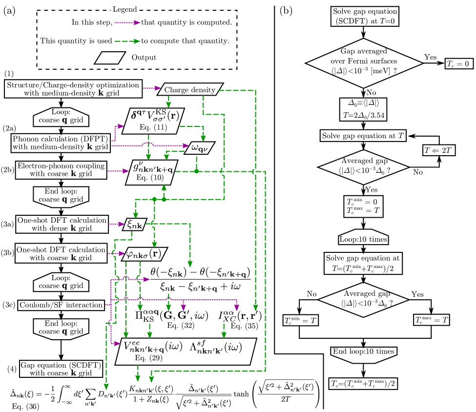
Figure 1: (a) The flow chart to perform the SCDFT calculation for each material in this study. The indices of steps are the same as those mentioned in Sec. III.4. (b) The flow chart of the bisection method used to compute $T_{c}$.

In this section, we will explain the practical procedure to perform the calculations explained in the previous section.

III.1 Evaluation of exchange integrals with Fourier transformation

The exchange integrals with Coulomb interaction part $V_{n{\bf k}n^{\prime}{\bf k}^{\prime}}^{ee}$ of Eq. (13) and the SF part $\Lambda_{n{\bf k}n^{\prime}{\bf k}^{\prime}}^{sf}$ of Eq. (22) can be computed efficiently using the Fourier transformation as follows: First $\rho^{(\alpha)}({\bf r})$ in Eqs. (14) and (17)-(19) has the periodicity of the lattice vector ${\bf R}$ together with the phase factor from the Bloch theorem as

$$\rho_{n{\bf k}n^{\prime}{\bf k}^{\prime}}^{(\alpha)}({\bf r}+{\bf R})=e^{i({\bf k}^{\prime}-{\bf k})\cdot{\bf R}}\rho_{n{\bf k}n^{\prime}{\bf k}^{\prime}}^{(\alpha)}({\bf r}).$$ (26)

Therefore $\rho^{(\alpha)}({\bf r})$ can be expanded with the Fourier components of the reciprocal lattice vectors ${\bf G}$ as

$$\rho_{n{\bf k}n^{\prime}{\bf k}+{\bf q}}^{(\alpha)}({\bf r})=\sum_{\bf G}e^{i({\bf q}+{\bf G})\cdot{\bf r}}{\tilde{\rho}}^{(\alpha)}_{n{\bf k}n^{\prime}{\bf k}+{\bf q}}({\bf G}),$$ (27)

where ${\tilde{\rho}}^{(\alpha)}({\bf G})$ is defined by the Fourier transformation of $\rho^{(\alpha)}({\bf r})$ as follows:

$${\tilde{\rho}}^{(\alpha)}_{n{\bf k}n^{\prime}{\bf k}+{\bf q}}({\bf G})\equiv\frac{1}{v_{\rm uc}}\int_{\rm uc}d^{3}re^{-i({\bf q}+{\bf G})\cdot{\bf r}}\rho_{n{\bf k}n^{\prime}{\bf k}+{\bf q}}^{(\alpha)}({\bf r}).$$ (28)

Subsequently, the exchange integral of Eq. (13) is rewritten as

$$V_{n{\bf k}n^{\prime}{\bf k}+{\bf q}}^{ee}(i\omega) =\sum_{{\bf G}{\bf G}^{\prime}}V_{RPA}^{\bf q}({\bf G},{\bf G}^{\prime},i\omega)$$

$$\hskip 28.45274pt\times{\tilde{\rho}}^{(0)}_{n{\bf k}n^{\prime}{\bf k}+{\bf q}}({\bf G}){\tilde{\rho}}^{(0)*}_{n{\bf k}n^{\prime}{\bf k}+{\bf q}}({\bf G}^{\prime}),$$ (29)

where $V_{RPA}^{\bf q}$ is the Fourier component of the screened Coulomb interaction as follows:

$$V_{RPA}^{\bf q}({\bf G},{\bf G}^{\prime},i\omega)$$

$$\equiv\iint d^{3}rd^{3}r^{\prime}e^{i({\bf q}+{\bf G})\cdot{\bf r}}e^{-i({\bf q}+{\bf G}^{\prime})\cdot{\bf r}^{\prime}}V_{RPA}({\bf r},{\bf r}^{\prime},i\omega).$$ (30)

However, the values of $V_{RPA}({\bf r},{\bf r}’,i\omega)$ need not be found, since we show that $V_{RPA}^{\bf q}({\bf G},{\bf G}^{\prime},i\omega)$ at each ${\bf q}$ can be computed separately using the Bloch theorem as shown below. By substituting $V_{RPA}({\bf r},{\bf r}^{\prime},i\omega)$ of Eq. (15) into Eq. (30), we obtain

$$V_{RPA}^{\bf q}({\bf G},{\bf G}^{\prime},i\omega)=\frac{4\pi\delta_{{\bf G}{\bf G}^{\prime}}}{|{\bf q}+{\bf G}|^{2}}$$

$$+\sum_{{\bf G}_{1}}V_{RPA}^{\bf q}({\bf G},{\bf G}_{1},i\omega)\Pi^{00{\bf q}}_{\rm KS}({\bf G}_{1},{\bf G}^{\prime},i\omega)\frac{4\pi}{|{\bf q}+{\bf G}^{\prime}|^{2}}$$

$$=\left[\frac{|{\bf q}+{\bf G}^{\prime}|^{2}\delta_{{\bf G}{\bf G}^{\prime}}}{4\pi}-\Pi^{00{\bf q}}_{\rm KS}({\bf G},{\bf G}^{\prime},i\omega)\right]^{-1},$$ (31)

where $\Pi^{\alpha\alpha{\bf q}}_{\rm KS}({\bf G},{\bf G}^{\prime},i\omega)$ is the Fourier component of the susceptibilities of the Kohn-Sham system of Eq. (16) given by

$$\Pi^{\alpha\alpha{\bf q}}_{\rm KS}({\bf G},{\bf G}^{\prime},i\omega)$$

$$\equiv\iint d^{3}rd^{3}r^{\prime}e^{i({\bf q}+{\bf G})\cdot{\bf r}}e^{-i({\bf q}+{\bf G}^{\prime})\cdot{\bf r}^{\prime}}\Pi^{\alpha\alpha}_{\rm KS}({\bf r},{\bf r}^{\prime},i\omega)$$

$$=\sum_{{\bf k}nn^{\prime}}\frac{\theta(-\xi_{n{\bf k}})-\theta(-\xi_{n^{\prime}{\bf k}+{\bf q}})}{\xi_{n{\bf k}}-\xi_{n^{\prime}{\bf k}+{\bf q}}+i\omega}{\tilde{\rho}}^{(\alpha)}_{n{\bf k}n^{\prime}{\bf k}+{\bf q}}({\bf G}){\tilde{\rho}}^{(\alpha)*}_{n{\bf k}n^{\prime}{\bf k}+{\bf q}}({\bf G}^{\prime}).$$ (32)

In the derivation of Eq. (31), we used the periodicity of each term with respect to the lattice vector. The factor $[\theta(-\xi_{n{\bf k}})-\theta(-\xi_{n^{\prime}{\bf k}+{\bf q}})]/(\xi_{n{\bf k}}-\xi_{n^{\prime}{\bf k}+{\bf q}}+i\omega)$ in the susceptibilities varies rapidly in the vicinity of Fermi surfaces, and we need a dense ${\bf k}$ grid to compute it accurately, which may require a huge numerical cost. Therefore, we use the reverse interpolation scheme explained in Sec. III.C.1 of Ref. Kawamura et al., 2017. In this scheme, we compute the explicitly energy-dependent factor with a dense ${\bf k}$ grid while we compute the other parts using a coarse ${\bf k}$ grid because ${\tilde{\rho}}^{(\alpha)}_{n{\bf k}n^{\prime}{\bf k}+{\bf q}}({\bf G}){\tilde{\rho}}^{(\alpha)*}_{n{\bf k}n^{\prime}{\bf k}+{\bf q}}({\bf G}^{\prime})$ varies more smoothly than the energy-dependent factor. The SF term can be computed in the same manner at each ${\bf q}$ separately. The Fourier component of the SF-mediated interaction of Eq. (23) is

$$\Lambda^{sf,\alpha\alpha}_{\bf q}({\bf G},{\bf G}^{\prime},i\omega)=-\sum_{{\bf G}_{1},{\bf G}_{2}}I_{XC}^{\alpha\alpha{\bf q}}({\bf G},{\bf G}_{1})$$

$$\times\left[\left(\Pi_{\rm KS}^{\alpha\alpha{\bf q}}({\bf G}_{1},{\bf G}_{2})\right)^{-1}-I_{XC}^{\alpha\alpha{\bf q}}({\bf G}_{1},{\bf G}_{2})\right]^{-1}I_{XC}^{\alpha\alpha{\bf q}}({\bf G}_{2},{\bf G}^{\prime}),$$ (33)

where $I_{XC}^{\alpha\alpha{\bf q}}$ is the Fourier component of the exchange correlation kernel of Eq. (25). In this study, we employed the local density approximation (LDA) to describe this kernel as follows: We approximate the exchange-correlation energy as

$$E_{XC}^{LDA}=\int d^{3}r\varepsilon_{XC}^{hom}(\rho({\bf r}),|{\bf m}({\bf r})|)\rho({\bf r}),$$ (34)

where $\rho({\bf r})$ is the electronic charge density and $\varepsilon_{XC}^{hom}(\rho,m)$ is the exchange-correlation energy density of the homogeneous electon gus whose charge and spin density are $\rho$ and $m$. The exchange-correlation kernel in Eq. (25) becomes

$$I_{XC}^{LDA,\alpha\alpha}({\bf r},{\bf r}^{\prime})$$

$$\hskip 8.5359pt=\delta({\bf r}-{\bf r}^{\prime})\rho({\bf r})\frac{\partial^{2}\varepsilon(\rho({\bf r}),|{\bf m}|)}{\partial{|\bf m|}\partial{|\bf m|}}\left.\left(\frac{m_{\alpha}}{|{\bf m}|}\right)^{2}\right|_{{\bf m}={\bf m}({\bf r})}.$$ (35)

Since we perform the non-magnetic calculation in this study, we take the ${\bf m}({\bf r})\rightarrow 0$ limit for this kernel. Within LDA, $I_{XC}^{\alpha\alpha{\bf q}}({\bf G},{\bf G}^{\prime})$ does not depend on ${\bf q}$. This is equivalent to the adiabatic local density approximation (ALDA) Gross and Kohn (1985) in time-dependent density functional theory Runge and Gross (1984).

III.2 Auxiliary gap equation

We have solved the gap equation (1) using the auxiliary energy axis Kawamura et al. (2017) to capture the rapid change of the explicitly energy-dependent function in the vicinity of Fermi surfaces. In this method, the gap function $\Delta_{n{\bf k}}$ depends also on the auxiliary energy; the auxiliary gap function ${\tilde{\Delta}}_{n{\bf k}}(\xi)$ satisfies ${\tilde{\Delta}}_{n{\bf k}}(\xi_{n{\bf k}})=\Delta_{n{\bf k}}$. Subsequently, the gap equation (1) becomes

$${\tilde{\Delta}}_{n{\bf k}}(\xi)=-\frac{1}{2}\int_{-\infty}^{\infty}d\xi^{\prime}\sum_{n^{\prime}{\bf k}^{\prime}}D_{n^{\prime}{\bf k}^{\prime}}(\xi^{\prime})\frac{K_{n{\bf k}n^{\prime}{\bf k}^{\prime}}(\xi,\xi^{\prime})}{1+Z_{n{\bf k}}(\xi)}$$

$$\times\frac{{\tilde{\Delta}}_{n^{\prime}{\bf k}^{\prime}}(\xi^{\prime})}{\sqrt{\xi^{\prime 2}+{\tilde{\Delta}}^{2}_{n^{\prime}{\bf k}^{\prime}}(\xi^{\prime})}}\tanh\left(\frac{\sqrt{\xi^{\prime 2}+{\tilde{\Delta}}^{2}_{n^{\prime}{\bf k}^{\prime}}(\xi^{\prime})}}{2T}\right),$$ (36)

where $D_{n{\bf k}}(\xi)$ is the $(n,{\bf k})$-resolved density of states. In the same manner, the electron-phonon and SF renormalization factors of Eqs. (6) and (21) become

$$Z_{n{\bf k}}^{ep}(\xi)=\frac{-1}{\tanh[\xi/(2T)]}\int_{-\infty}^{\infty}d\xi^{\prime}\sum_{n^{\prime}{\bf k}^{\prime}\nu}D_{n^{\prime}{\bf k}^{\prime}}(\xi^{\prime})|g_{n{\bf k}n^{\prime}{\bf k}^{\prime}}^{\nu}|^{2}$$

$$\times[J(\xi,\xi^{\prime},\omega_{{\bf k}^{\prime}-{\bf k}\nu})+J(\xi,-\xi^{\prime},\omega_{{\bf k}^{\prime}-{\bf k}\nu})]$$ (37)

and

$$Z_{n{\bf k}}^{sf}(\xi)=\frac{1}{\pi}\int_{-\infty}^{\infty}d\xi^{\prime}\sum_{n^{\prime}{\bf k}^{\prime}}D_{n^{\prime}{\bf k}^{\prime}}(\xi^{\prime})\int_{0}^{\infty}d\omega$$

$$\times\frac{(|\xi|+|\xi_{n^{\prime}{\bf k}^{\prime}}|)^{2}-\omega^{2}}{[(|\xi|+|\xi_{n^{\prime}{\bf k}^{\prime}}|)^{2}+\omega^{2}]^{2}}\Lambda_{n{\bf k}n^{\prime}{\bf k}^{\prime}}^{sf}(i\omega),$$ (38)

respectively, where we employ the reverse interpolation method again; the $(n,{\bf k})$-resolved density of states $D_{n{\bf k}}(\xi)$ is computed with the dense ${\bf k}$ grid, while the other parts are computed on the coarse ${\bf k}$ grid; finally, we combine the parts yielded.

III.3 Frequency integral

The integration in Eq. (12) involves the frequency $\omega$ spanning [0,$\infty$]. Therefore, to perform the integration numerically, we change the variable as follows:

$$\omega=(|\xi|+|\xi^{\prime}|)\frac{1+x}{1-x}.$$ (39)

Then Eq. (12) becomes

$$K_{n{\bf k}n^{\prime}{\bf k}^{\prime}}^{ee}(\xi,\xi^{\prime})=\frac{2}{\pi}\int_{-1}^{1}dx\frac{1}{1+x^{2}}$$

$$\times V_{n{\bf k}n^{\prime}{\bf k}^{\prime}}^{ee}\left(i(|\xi|+|\xi^{\prime}|)\frac{1+x}{1-x}\right).$$ (40)

When $|\xi|+|\xi^{\prime}|=0$, this integration becomes $V_{n{\bf k}n^{\prime}{\bf k}^{\prime}}^{ee}(0)$. To obtain $V_{n{\bf k}n^{\prime}{\bf k}^{\prime}}^{ee}(i\omega)$ at an arbitrary $\omega$, we first compute $V_{n{\bf k}n^{\prime}{\bf k}^{\prime}}^{ee}(i\omega)$ at discrete non-uniform points $\omega=0,\omega_{1},\omega_{2},\cdots,\infty$ and interpolate them. Using the same transformation as in Eq. (39), the frequency integral in the SF renormalization term (38) is performed as follows:

$$Z_{n{\bf k}}^{sf}(\xi) =\frac{1}{\pi}\int_{-\infty}^{\infty}d\xi^{\prime}\sum_{n^{\prime}{\bf k}^{\prime}}D_{n^{\prime}{\bf k}^{\prime}}(\xi^{\prime})$$

$$\int_{-1}^{1}dx\frac{-2x}{(|\xi|+|\xi_{n^{\prime}{\bf k}^{\prime}}|)(1+x^{2})^{2}}$$

$$\times\Lambda_{n{\bf k}n^{\prime}{\bf k}^{\prime}}^{sf}\left(i(|\xi|+|\xi^{\prime}|)\frac{1+x}{1-x}\right).$$ (41)

The numerical integration with respect to the variable $x$ ranging [-1,1] can be performed using the Gauss quadrature.

III.4 Overall procedure

Figure 1 (a) shows the calculation flow. We employ the following three different wavenumber grids to efficiently perform the Brillouin-zone integrals:

coarse grid

To reduce the computational cost, we use a coarse grid for the wavenumber ${\bf q}$ of phonons and susceptibilities. The grid is shifted by half of its step to avoid the singularity at the $\Gamma$ point. This grid is also used for solving the gap equation.

medium-density grid

The atomic structure and the charge density are optimized with the self-consistent field calculation using ${\bf k}$ grid denser than the coarse grid. This ${\bf k}$ grid is used to prepare electronic states in the DFPT calculation.

dense grid

To treat the explicitly energy-dependent factor in the calculations of susceptibilities and the ($n,{\bf k}$)-dependent density of states in the gap equation (36), a dense ${\bf k}$ grid is employed.

The overall calculations are performed as follows:

1. First, we optimize the atomic structure and the charge density using the standard density functional calculation with the medium-density ${\bf k}$ grid. The following calculation is performed on this optimized atomic structure and with the charge density.

2. We compute the electron-phonon interaction and the frequency of phonons, whose wavenumber ${\bf q}$ is on the half-grid shifted coarse grid. This step is further split into the following two sub-steps:

   1. The phonon calculation based on DFPT is performed; the electronic states used in this calculation have a wavenumber ${\bf k}$ on the medium-density grid.

   2. Electron-phonon vertex of Eq. (10) between the Kohn-Sham orbitals $(n,{\bf k})$ and $(n^{\prime},{\bf k}+{\bf q})$ is computed, where the wavenumber ${\bf k}$ is on the coarse grid.

3. Next, we compute the exchange integrals of screened Coulomb and SF-mediated interaction whose transitional momentum ${\bf q}$ is on the half-grid shifted coarse grid. This step is split into the following three sub-steps:

   1. One-shot DFT calculation on the dense ${\bf k}$ grid is performed. The resulting energy dispersion $\xi_{n{\bf k}}$ is later used to compute the explicitly energy-dependent term in the susceptibilities in Eq. (32).

   2. One-shot DFT calculation on the coarse ${\bf k}$ grid with and without a half-grid shift is performed. These two grids are connected by the transitional momentum ${\bf q}$ on the coarse a half-grid shifted grid. The resulting Kohn-Sham orbitals will be used to compute $\rho^{(\alpha)}({\bf r})$ of Eqs. (14) and (17)-(19).

   3. The exchange integrals of screened Coulomb and SF-mediated interaction between the Kohn-Sham orbitals $(n,{\bf k})$ and $(n^{\prime},{\bf k}+{\bf q})$ are computed, where the wavenumber ${\bf k}$ is on the coarse grid.

4. The gap equation within SCDFT is solved on the coarse ${\bf k}$ grid at each temperature. Then $T_{c}$ is obtained as a minimum temperature where all $\Delta_{n{\bf k}}(\xi)$ vanish.

The transition temperature $T_{c}$ is found using the bisection method explained in Fig. 1 (b). While the initial lower limit of $T_{c}$ is set to zero, the initial upper limit is set to the $T_{c}$ estimated by the Bardeen-Cooper-Schrieffer theory Bardeen et al. (1957); Schrieffer (1983) ($2\Delta_{0}/3.54$, where $\Delta_{0}$ is the superconducting gap averaged over Fermi surfaces at zero kelvin). If there is a finite gap even at this upper limit, although it rarely occurs, we double the initial upper limit; then we repeat the bisection step ten times and find $T_{c}$.

IV Result

Table 1: Structure, cutoff for the plane wave for wave functions, ${\bf q}$-grid for phonon, and the error of the lattice constant $\langle\Delta a/a_{\rm exp}\rangle\equiv(V_{\rm calc}/V_{\rm exp})^{1/3}-1$. $V_{\rm calc}$ and $V_{\rm exp}$ are the calculated and experimental unit-cell volume, respectively.

	structure	cutoff [Ry]	coarse grid	$\langle\Delta a/a_{\rm exp}\rangle$ [%]
Be	hcp	65	$10\times 10\times 5$	-0.74
Na	bcc	90	$6\times 6\times 6$	-0.60
Mg	hcp	65	$7\times 7\times 4$	-0.77
Al	fcc	65	$8\times 8\times 8$	-0.90
K	bcc	120	$5\times 5\times 5$	0.61
Ca	fcc	120	$6\times 6\times 6$	-1.20
Sc	hcp	45	$7\times 7\times 4$	-0.49
Ti	hcp	50	$7\times 7\times 4$	-0.28
V	bcc	100	$9\times 9\times 9$	-1.19
Cu	fcc	90	$9\times 9\times 9$	0.42
Zn	hcp	90	$8\times 8\times 4$	-0.02
Ga	$\alpha$-Ga	150	$5\times 5\times 4$	1.35
Rb	bcc	30	$5\times 5\times 5$	0.58
Sr	fcc	30	$5\times 5\times 5$	-1.09
Y	hcp	40	$6\times 6\times 3$	0.94
Zr	hcp	50	$7\times 7\times 4$	0.09
Nb	bcc	90	$8\times 8\times 8$	0.53
Mo	bcc	35	$8\times 8\times 8$	0.44
Tc	hcp	30	$8\times 8\times 4$	0.04
Ru	hcp	35	$8\times 8\times 4$	-0.62
Rh	fcc	35	$8\times 8\times 8$	0.73
Pd	fcc	45	$8\times 8\times 8$	1.18
Ag	fcc	50	$8\times 8\times 8$	1.42
Cd	hcp	45	$7\times 7\times 3$	2.32
In	bct	65	$7\times 7\times 7$	1.84
Sn	$\beta$-Sn	50	$7\times 7\times 7$	1.72
Cs	bcc	75	$4\times 4\times 4$	1.01
Ba	bcc	30	$5\times 5\times 5$	-0.19
La	hcp	120	$6\times 6\times 3$	0.60
Hf	hcp	55	$7\times 7\times 4$	0.01
Ta	bcc	50	$8\times 8\times 8$	0.79
W	bcc	50	$8\times 8\times 8$	0.62
Re	hcp	60	$8\times 8\times 4$	0.39
Os	hcp	55	$8\times 8\times 4$	1.00
Ir	fcc	40	$8\times 8\times 8$	1.29
Pt	fcc	60	$8\times 8\times 8$	1.15
Au	fcc	45	$8\times 8\times 8$	1.15
Hg	trigonal	50	$6\times 6\times 6$	6.81
Tl	hcp	55	$6\times 6\times 3$	3.10
Pb	fcc	35	$6\times 6\times 6$	1.77

In this section we will first explain the numerical condition of this study, then show the result of the benchmark.

The numerical condition is as follows: We use the DFT code Quantum ESPRESSO Giannozzi et al. (2017) which employs plane waves and pseudopotentials. Perdew-Burke-Ernzerhof’s density functional Perdew et al. (1997) based on generalized gradient approximation (GGA) is used. We use the optimized norm-conserving pseudopotential Hamann (2013) library provided by Schlipf-Gygi (SG15) Schlipf and Gygi (2015); Prandini et al. (2018). The energy cutoff for the wave functions of each element is specified using the criteria and the convergence profiles in the Standard Solid State Pseudopotentials Prandini et al. (2018). We are using the optimized tetrahedron method Kawamura et al. (2014) to perform the Brillouin-zone integration. The number of grids along each reciprocal lattice vector is proportional to the length of that vector. Table 1 presents the above explained conditions for each element. The SCDFT calculation is performed using the Superconducting Toolkit Sup software package. We have set the medium-density grid twice the density of the coarse grid and set the dense grid twice the density of the medium-density grid; for example, $8^{3}$, $16^{3}$, and $32^{3}$ grids were used for the coarse, medium-density, and dense grids, respectively; all for Al. The minimum scale and the number of points of the non-uniform auxiliary energy grid used in the gap equation (36) were set to $10^{-7}$ Ry and 100, respectively. In the calculation of the magnetic exchange-correlation kernel of Eq. (25), we ignore the gradient correction. For stabilizing the phonon calculation, the lattice constants and the internal atomic coordinates are optimized; the deviation between the optimized and the experimental lattice constants are listed in Tbl. 1. To compute the susceptibilities in Eq. (32) and solve the gap equation (36), we have included $40\times N_{\rm atom}$ ($20\times N_{\rm atom}$) empty bands for the calculation with (without) SOI, where $N_{\rm atom}$ is the number of atoms per unit cell.

Figure 2: The experimental $T_{c}$ ($T_{c}^{\rm exp}$) Hamlin (2015) and the theoretical $T_{c}$ computed with and without SOI/SF. In addition, we show the density of states (DOS) divided by the number of atoms, the averaged phonon frequencies $\omega_{\rm ln}$, the Fröhlich’s mass-enhancement parameter $\lambda$, the averaged Coulomb interaction $\mu_{\rm C}$ in Eq. (46), and the averaged SF term $\mu_{s}$ in Eq. (47). Cyan, green, red, blue, and yellow cells indicate the alkaline (earth) metals, the sp-orbital metals, the group 12 metals, the noble metals, and the other transition metals, respectively.

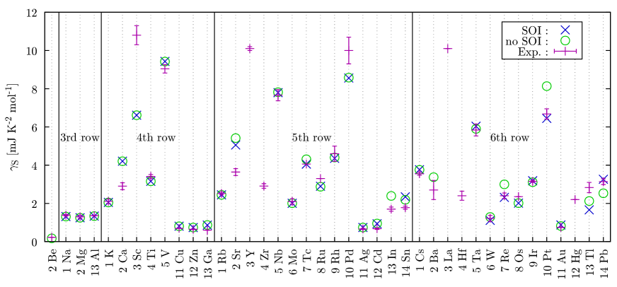
Figure 3: Theoretical and experimental Gschneidner (1964) Sommerfeld coefficient $\gamma_{\rm S}$. The horizontal axis is the atomic symbol together with the group of the periodic table. Blue crosses and green circles indicate the Sommerfeld coefficient computed with and without SOI while magenta “+” with an error bar indicates the experimental value of the Sommerfeld coefficient.

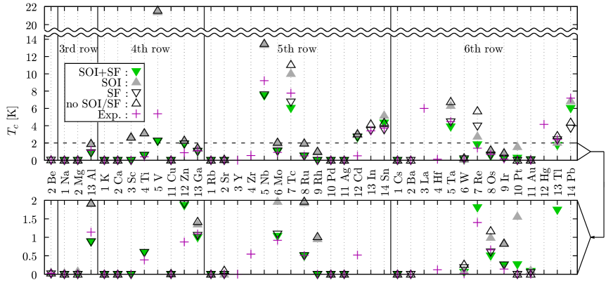
Figure 4: Theoretical and experimental $T_{c}$s. The horizontal axis is the atomic symbol together with the group of the periodic table. Downward (upward) triangles indicate the $T_{c}$s computed with (without) SF. Filled (empty) triangles indicate the $T_{c}$s computed with (without) SOI. “+” indicates the experimental value of $T_{c}$. The plot which ranges from zero to two Kelvin in the upper panel is magnified into the bottom panel.

Next, we move onto the results. Figure 2 shows the experimental $T_{c}$ ($T_{c}^{\rm exp}$) Hamlin (2015), the theoretical $T_{c}$ computed with and without SOI/SF in a periodic-table form. Also, to examine the effects of the electron-phonon interaction, the screened Coulomb repulsion, and the spin-fluctuation, we are showing the following quantities in the same figure: The density of states (DOS) at the Fermi level divided by the number of atoms affects the strength of the mean-field. The Fröhlich’s mass-enhancement parameter

$$\lambda=\sum_{{\bf q}\nu}\lambda_{{\bf q}\nu},$$ (42)

and the averaged phonon frequencies

$$\omega_{\rm ln}=\exp\left[\frac{1}{\lambda}\sum_{{\bf q}\nu}\lambda_{{\bf q}\nu}\ln(\omega_{{\bf q}\nu})\right],$$ (43)

appear in the conventional McMillan formula McMillan (1968); Dynes (1972)

$$T_{c}=\frac{\omega_{\rm ln}}{1.2}\exp\left[\frac{-1.04(1+\lambda)}{\lambda-\mu^{*}(1+0.62\lambda)}\right]$$ (44)

which has been used to estimate $T_{c}$ semi-empirically with an adjustable parameter $\mu^{*}$. The $({\bf q},\nu)$-dependent mass-enhancement parameter $\lambda_{{\bf q}\nu}$ is computed as follows:

$$\lambda_{{\bf q}\nu}=\frac{2}{D(0)\omega_{{\bf q}\nu}}\sum_{{\bf k}nn^{\prime}}|g_{n{\bf k}n^{\prime}{\bf k}+{\bf q}}^{\nu}|^{2}\delta(\xi_{n{\bf k}})\delta(\xi_{n^{\prime}{\bf k}+{\bf q}}),$$ (45)

where $D(0)$ is the density of states at the Fermi level. We are calculating here the Brillouin-zone integral, including two delta functions, using the dense ${\bf k}$ grid together with the optimized tetrahedron method Kawamura et al. (2014). Because of the double delta function $\delta(\xi_{n{\bf k}})\delta(\xi_{n^{\prime}{\bf k}+{\bf q}})$, this summation involves the electron-phonon vertices only between the electronic states at the Fermi level. Therefore, the Fröhlich’s mass-enhancement parameter $\lambda$ in Eq. (42) indicates the retarded phonon-mediated interaction ($2|g|^{2}/\omega$) averaged over Fermi surfaces times the density of state at the Fermi level. Similarly, $\omega_{\rm ln}$ indicates the typical frequency of phonons which couples largely with the electronic states at the Fermi level. Therefore, $\lambda$ and $\omega_{\rm ln}$ closely relate to the electron-phonon contribution to $T_{c}$. In an analogous fashion to $\lambda$, we are showing parameters for the Coulomb repulsion and SF as

$$\mu_{\rm C}=\frac{1}{D(0)}\sum_{{\bf k}{\bf k}^{\prime}nn^{\prime}}K_{n{\bf k}n^{\prime}{\bf k}^{\prime}}^{ee}\delta(\xi_{n{\bf k}})\delta(\xi_{n^{\prime}{\bf k}^{\prime}}),$$ (46)

and

$$\mu_{s}=\frac{1}{D(0)}\sum_{{\bf k}{\bf k}^{\prime}nn^{\prime}}K_{n{\bf k}n^{\prime}{\bf k}^{\prime}}^{sf}\delta(\xi_{n{\bf k}})\delta(\xi_{n^{\prime}{\bf k}^{\prime}}),$$ (47)

respectively. These parameters are the Coulomb [Eq.(12)] and SF [Eq.(20)] kernels averaged over Fermi surfaces times the density of states at the Fermi level.

We note that in Fig. (2), some results are absent because of the following reason: Li has a vast unit cell at a low temperature, and it is computationally demanding. Cr, Mn, Fe, Co, and Ni show a magnetic order at the low temperature. Therefore, the formalism of the spin-fluctuation (23) used in this study breaks down; the matrix

$$\delta_{{\bf G}{\bf G}^{\prime}}-\sum_{{\bf G}_{1}}\Pi_{\rm KS}^{\alpha\alpha{\bf q}}({\bf G},{\bf G}_{1})I_{XC}^{\alpha\alpha{\bf q}}({\bf G}_{1},{\bf G}^{\prime})$$ (48)

does not become positive definite (the Stoner’s criterion) for those materials. For Be and Ba, there is no pseudopotential together with SOI in the pseudopotential library used in this study. Since we are trying to unify the condition of the calculation for all elements, we leave the result of these two materials together with SOI blank. For Y, Zr, In (with SOI), La, Hf, and Hg, we have obtained imaginary phonon frequencies because of an artificial long-range structure instability. For such cases, we could have not continue the calculation because of the breakdown of the formulations of the electron-phonon kernel [Eq. (5)] and renormalization term [Eq. (6)]. Therefore, we leave the results for those cases blank.

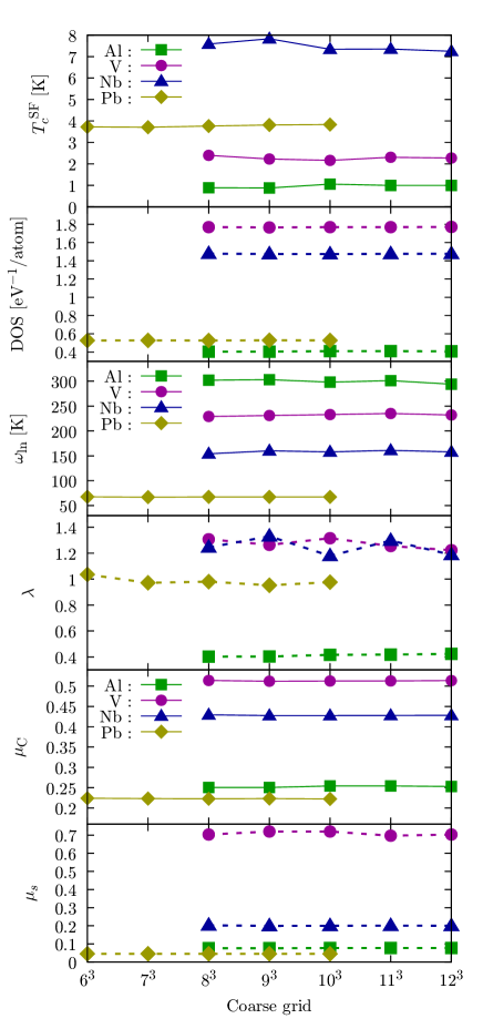
Figure 5: The convergence of calculated $T_{c}$ (with SF, without SOI), the density of states at the Fermi level, the averaged phonon frequencies $\omega_{\rm ln}$, the Fröhlich’s mass-enhancement parameter $\lambda$, he averaged Coulomb interaction $\mu_{\rm C}$ in Eq. (46), and the averaged SF term $\mu_{s}$ in Eq. (47) with respect to the density of the wave-number grids. We pick up Al, V, Nb, and Pb.

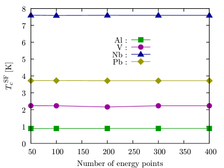
Figure 6: The convergence of the $T_{c}$ (with SF) with respect to the number of points for the energy integral in Eq. (36) for Al, V, Nb, and Pb.

We have checked the convergences of the numerical results with respect to the density of ${\bf k}$, ${\bf q}$, and the auxiliary energy grids. For this purpose, we have selected up the typical four materials, namely Al, V, Nb, and Pb. Figure 5 shows the convergence of calculated $T_{c}$ (with SF, without SOI), the density of states at the Fermi level, the averaged phonon frequencies $\omega_{\rm ln}$, the Fröhlich’s mass-enhancement parameter $\lambda$, he averaged Coulomb interaction $\mu_{\rm C}$ in Eq. (46), and the averaged SF term $\mu_{s}$ in Eq. (47) with respect to the density of the wave-number grids. Also, in the convergence check, we have set the medium-density grid twice the density of the coarse grid and have set the dense grid twice the density of the medium-density grid. Although the $\lambda$ of V and Nb oscillate within 4% and 7%, respectively, when we change the density of the coarse grid, other quantities, including $T_{c}$, are unchanged. We are showing the convergence of $T_{c}$ (with SF, without SOI) with respect to the number of points for the energy integral in Eq. (36) in Fig. 6. This result shows the $T_{c}$s have converged at the numerical conditions described above.

We compare $\lambda$ in Eq. (42), $\omega_{\rm ln}$ in Eq. (43), and $\mu_{\rm C}$ in Eq. (46) obtained in this study and earlier studies. Table 2 shows $\lambda$ and $\omega_{\rm ln}$ in this study and earlier studies. Although there are small deviations due to the different exchange-correlation functional, these quantities are consistent with those of earlier studies excepting the case for Pb without SOI; the reported $\lambda$s of Pb without SOI are scattered and different from the experimental value ($\lambda_{\rm exp}=1.55$) McMillan and Rowell (1969). We also confirm that we reproduced the averaged Coulomb interaction $\mu_{\rm C}$ in Eq. (46) in the earlier works for Al and Nb; $\mu_{\rm C}$ is 0.251 and 0.429 for Al and Nb, respectively in this study while those in the earlier studies are 0.236 Lee et al. (1995) and 0.488 Lee and Chang (1996).

Table 2: Fröhlich’s mass-enhancement parameter $\lambda$ in Eq. (42) and the averaged phonon frequencies $\omega_{\rm ln}$ in Eq. (43) computed in this study and earlier studies. Numerical conditions, the ${\bf q}$ grid of phonons, the ${\bf k}$ grid of electronic states for the calculation of phonon frequencies, the ${\bf k}$ grid and the smearing width for the integration in Eq. (45) are also written. In the Ref. Liu and Quong, 1996 only the number of ${\bf q}$ and ${\bf k}$ points in the irreducible Brillouin-zone (IBZ) are provided. In this study and one of the earlier studies Savrasov and Savrasov (1996) the tetrahedron method is employed for performing the Brillouin-zone integration in Eq. (45).

	$\lambda$	$\omega_{\rm ln}$ [K]	${\bf q}$ grid	${\bf k}$ grid (phonon)	${\bf k}$ grid ($\lambda$)	Smearing [eV]	Functional	Ref.
Al (without SOI)	0.402	302	$8\times 8\times 8$	$16\times 16\times 16$	$32\times 32\times 32$	Tetrahedron	GGA	This work
	0.438	-	89 in IBZ	-	1,300 in IBZ	0.272	LDA	Liu and Quong,1996
	0.417	314	$8\times 8\times 8$	$12\times 12\times 12$	$32\times 32\times 32$	0.272	LDA	Akashi and Arita,2013
	0.44	270	$8\times 8\times 8$	$16\times 16\times 16$	$32\times 32\times 32$	Tetrahedron	LDA	Savrasov and Savrasov,1996
V (without SOI)	1.26	231	$9\times 9\times 9$	$18\times 18\times 18$	$36\times 36\times 36$	Tetrahedron	GGA	This work
	1.19	245	$8\times 8\times 8$	$16\times 16\times 16$	$32\times 32\times 32$	Tetrahedron	LDA	Savrasov and Savrasov,1996
Cu (without SOI)	0.119	216	$9\times 9\times 9$	$18\times 18\times 18$	$36\times 36\times 36$	Tetrahedron	GGA	This work
	0.14	220	$8\times 8\times 8$	$16\times 16\times 16$	$32\times 32\times 32$	Tetrahedron	LDA	Savrasov and Savrasov,1996
Nb (without SOI)	1.24	154	$8\times 8\times 8$	$16\times 16\times 16$	$32\times 32\times 32$	Tetrahedron	GGA	This work
	1.26	185	$8\times 8\times 8$	$16\times 16\times 16$	$32\times 32\times 32$	Tetrahedron	LDA	Savrasov and Savrasov,1996
Mo (without SOI)	0.438	265	$8\times 8\times 8$	$16\times 16\times 16$	$32\times 32\times 32$	Tetrahedron	GGA	This work
	0.42	280	$8\times 8\times 8$	$16\times 16\times 16$	$32\times 32\times 32$	Tetrahedron	LDA	Savrasov and Savrasov,1996
Pd (without SOI)	0.333	145	$8\times 8\times 8$	$16\times 16\times 16$	$32\times 32\times 32$	Tetrahedron	GGA	This work
	0.35	180	$8\times 8\times 8$	$16\times 16\times 16$	$32\times 32\times 32$	Tetrahedron	LDA	Savrasov and Savrasov,1996
Ta (without SOI)	0.923	149	$8\times 8\times 8$	$16\times 16\times 16$	$32\times 32\times 32$	Tetrahedron	GGA	This work
	0.86	160	$8\times 8\times 8$	$16\times 16\times 16$	$32\times 32\times 32$	Tetrahedron	LDA	Savrasov and Savrasov,1996
Tl (without SOI)	1.03	47	$6\times 6\times 3$	$12\times 12\times 6$	$24\times 24\times 12$	Tetrahedron	GGA	This work
	1.0	-	$8\times 8\times 8$	$24\times 24\times 16$	$36\times 36\times 24$	0.2	LDA	Heid et al.,2010
Tl (with SOI)	0.752	47	$6\times 6\times 3$	$12\times 12\times 6$	$24\times 24\times 12$	Tetrahedron	GGA	This work
	0.87	-	$8\times 8\times 8$	$24\times 24\times 16$	$36\times 36\times 24$	0.2	LDA	Heid et al.,2010
Pb (without SOI)	1.04	67	$6\times 6\times 6$	$12\times 12\times 12$	$24\times 24\times 24$	Tetrahedron	GGA	This work
	1.20	-	89 in IBZ	-	1,300 in IBZ	0.272	LDA	Liu and Quong,1996
	1.68	65	$8\times 8\times 8$	$16\times 16\times 16$	$32\times 32\times 32$	Tetrahedron	LDA	Savrasov and Savrasov,1996
	1.08	-	$8\times 8\times 8$	$16\times 16\times 16$	$32\times 32\times 32$	0.2	LDA	Heid et al.,2010
	1.24	-	$8\times 8\times 8$	$16\times 16\times 16$	$40\times 40\times 40$	0.272	LDA	Margine and Giustino,2013
Pb (with SOI)	1.45	58	$6\times 6\times 6$	$12\times 12\times 12$	$24\times 24\times 24$	Tetrahedron	GGA	This work
	1.56	-	$8\times 8\times 8$	$16\times 16\times 16$	$32\times 32\times 32$	0.2	LDA	Heid et al.,2010

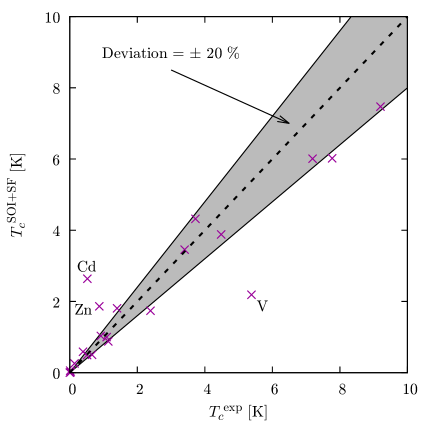
Figure 7: Experimental and computed $T_{c}$. For the theoretical value, only the result computed with SOI and SF is represented. The shaded region indicates that the deviation of $T_{c}$ ($T_{c}^{\rm SOI+SF}/T_{c}^{\rm exp}$) is less than 20 %.

In Fig. 7, we have plotted the experimental $T_{c}$ together with the $T_{c}$ calculated the most precisely in this work by including SOI and SF. We note that since there is no computed data for Be and In with SOI, we are showing the data for them without SOI. Excepting Cd, Zn, and V, we have accurately reproduced experimental $T_{c}$. Inside the target elements of this benchmark, the three highest-$T_{c}$ elements observed experimentally are Nb (9.20 K), Tc (7.77 K), and Pb (7.19 K). Also, the three highest-$T_{c}$ elements in our calculation are Nb (7.470 K), Tc (6.019 K), and Pb (6.010 K). Therefore, at least in the elemental metals at ambient pressure, we can predict the highest-$T_{c}$ materials.

V Discussion

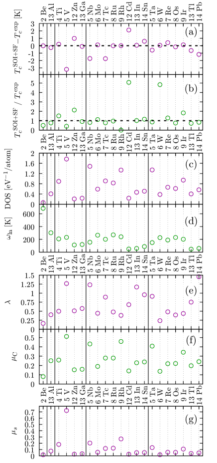
Figure 8: We plot the following quantities for the elemental systems which have finite $T_{c}$: (a) The difference between the experimental $T_{c}$ ($T_{c}^{\rm exp}$) and theoretical $T_{c}$ computed with SOI and SF ($T_{c}^{\rm SOI+SF}$). (b) The ratio between $T_{c}^{\rm exp}$ and $T_{c}^{\rm SOI+SF}$. (c) The density of states at the Fermi level. (d) The averaged phonon frequencies $\omega_{\rm ln}$. (e) The Fröhlich’s mass-enhancement parameter $\lambda$. (f) The averaged Coulomb interaction $\mu_{\rm C}$ in Eq. (46). (g) The averaged SF term $\mu_{s}$ in Eq. (47). The horizontal axis is the atomic symbol together with the group of the periodic table. We note that since there is no computed data for Be and In with SOI, we show the data for them without SOI.

In this section, we discuss the results shown in the previous section. To check the accuracy of the calculation of the electron-phonon interaction, we will plot in Fig. 3 the calculated- and experimental- Gschneidner (1964) Sommerfeld coefficient $\gamma_{\rm S}$ which is the prefactor of the specific heat at a low temperature

$$C_{v}=\gamma_{\rm S}T+O(T^{3}).$$ (49)

This coefficient is estimated using the density of states and the Fröhlich’s mass-enhancement parameter as follows

$$\gamma_{\rm S}=\frac{\pi^{2}D(0)}{3}(1+\lambda).$$ (50)

The calculated $\gamma_{\rm S}$ agrees very well with the experimental value. For Re, Pt, and Pb, this agreement becomes improved by including SOI; Since these heavy elements have large SOI, this interaction is crucial to reproduce the experimental Sommerfeld coefficient.

We have plotted the computed- and experimental-$T_{c}$ data contained in Fig. 2 into Fig. 4 to visualize the effect by SOI and SF; we can detect the following trends by inspecting this graph: SF always reduces $T_{c}$s for the elemental systems. This reduction becomes significant for the transition metals and is crucial to reproduce the experimental $T_{c}$ quantitatively. The mechanism of this reduction is explained as follows Berk and Schrieffer (1966); Tsutsumi et al. : For isotropic superconductors such as elemental materials, ferromagnetic spin-fluctuation becomes dominant and aligns the spin of electrons parallel. This effect breaks the singlet Cooper pair in the isotropic superconductors. On the other hand, in cuprates and iron-based superconductors, highly anisotropic antiferromagnetic spin-fluctuation becomes dominant and enhances the superconducting gaps with sign-changes Essenberger et al. (2016). In the transition metals, the effect of SF weakens with the increasing of the period number in the periodic table. For example, $\mu_{s}$ varies 0.722 (V) $\rightarrow$ 0.203 (Nb) $\rightarrow$ 0.131 (Ta), 0.057 (Mo) $\rightarrow$ 0.018 (W), 0.117 (Tc) $\rightarrow$ 0.057 (Re), 0.122 (Ru) $\rightarrow$ 0.055 (Os), and 0.269 (Rh) $\rightarrow$ 0.108 (Ir). Also, the $\mu_{s}$ of Pd becomes negative; this indicates the formulation of SF breaks down due to the magnetic order. Although the magnetic order is a numerical artifact, this result shows that Pd has larger SF than that of Pt. This trend of SF can be explained as follows Tsutsumi et al. : The electronic orbitals become delocalized with the increasing of the principal quantum number (3d $\rightarrow$ 4d $\rightarrow$ 5d); this delocalization decreases the magnetic exchange-correlation kernel in Eq. (25); also, the delocalized orbital has small DOS. Therefore, the elements with the larger period number exhibit smaller SF contribution. We cannot see this trend in the alkaline metals. For these elements, $\mu_{s}$ does not decrease with the increasing of the period number, i.e., this parameter varies 0.213 (Na) $\rightarrow$ 0.270 (K) $\rightarrow$ 0.280 (Rb) $\rightarrow$ 0.427 (Cs). This behavior comes from the increasing of DOS because of the larger lattice constant (larger atomic radius) for the alkaline metals having the larger period numbers. The effect of SOI is small in most cases, excepting Tc, Sn, Re, Tl, Pb. In these elements, the Fröhlich’s parameter $\lambda$ changes drastically by turning on the SOI. For Pb, this enhancement of $\lambda$ (1.036 $\rightarrow$ 1.453) can be traced back to the three contributions i.e., the phonon softening ($\omega_{\rm ln}$ decreases from 67 K to 58 K), the increased DOS at Fermi level (0.527 eV^-1 $\rightarrow$ 0.564 eV^-1), and the enhanced deformation potential ${\bm{\delta}}^{{\bf q}\tau}V_{\rm KS}({\bf r})$ due to the SOI term Heid et al. (2010). These effects of SOI in Tc, Re, and Tl are opposite to ones in Pb and Sn; SOI reduces the electron-phonon coupling as well as $T_{c}$ in these three materials. We can reproduce the absence of the superconductivity in alkaline, alkaline earth, and noble metals, excepting Pt and Au with SOI and SF; we have observed small finite $T_{c}$ for these two elements; we can reproduce the non-superconductivity also in Sc by including SF while we observe $T_{c}=2.711$ K by ignoring SF. Since Sc has highly localized 3d electrons, the SF largely reduces $T_{c}$. For the group 12 elements (Zn and Cd), $T_{c}$s are overestimated even if we include SF. For these materials, the SF effect is small because the d orbitals are fully occupied.

Finally, we have tried to find the factor which dominates the accuracy of $T_{c}$. In Fig. 8, we have plottd the following quantities for the elemental systems with finite $T_{c}$: (a) The difference between the experimental $T_{c}$ ($T_{c}^{\rm exp}$) and theoretical $T_{c}$ computed with SOI and SF ($T_{c}^{\rm SOI+SF}$). (b) The ratio between $T_{c}^{\rm exp}$ and $T_{c}^{\rm SOI+SF}$. (c) The density of states at the Fermi level. (d) The averaged phonon frequencies $\omega_{\rm ln}$ in Eq. (43). (e) The Fröhlich’s mass-enhancement parameter $\lambda$ in Eq. (42). (f) The averaged Coulomb interaction $\mu_{\rm C}$ in Eq. (46). (g) The averaged SF term $\mu_{s}$ in Eq. (47). Note that since there is no computed data for Be and In with SOI, we are presenting data for these two elements without SOI. $T_{c}$s of Zn and Cd (V, Nb, Tc, Pb) are overestimated (underestimated) in the differential plot (a) while those of Zn Cd, W, Ir (Be, V, Rh) are overestimated (underestimated) in the ratio plot (b). Therefore, for V, Zn, and Cd, the focus should be on examining the accuracy of $T_{c}$; therefore, we attempted to find features of these three materials from elemental systems. From Fig. 8 (g), we can see that V has extremely large $\mu_{s}$. When the system has large SF, the SF-mediated interaction in Eq. (33) changes rapidly because the inverse of the matrix in Eq. (48) approaches to a singular matrix. Therefore, the SF of such systems needs to computed more precisely, for example, by including the gradient collection into the magnetic exchange-correlation kernel in Eq. (25). However, it is difficult to identify the significant difference between Zn, Cd, and other materials. For example, the parameters of Ga are extremely close to those of Zn. However, the calculated $T_{c}$ of Ga is in good agreement with the experimental one.

By leaving from the superconductivity, we can see the following features from Fig. 8: DOS and $\mu_{C}$ are showing very similar behavior. Since $\mu_{C}$ in Eq. (46) can be approximated to the DOS times the averaged Coulomb interaction, the synchronicity indicates that the elemental materials in Fig. 8 have nearly the same screened Coulomb repulsion. $\omega_{\rm ln}$ has peaks around group 6-9 on both periods 5 and 6. Additionally, the frequencies at both the peaks are extremely close, although the atomic masses of these periods are different; these behaviors can be explained by the following Friedel’s theory Friedel (1967). The materials in groups 6-9 have high cohesive energy because of the half-filled d-orbitals; the high cohesive energy leads to the hardness and the high phonon frequencies of the materials. Since 5d orbitals are more delocalized than 4d orbitals, the binding energy increases for 5d materials. Therefore, the phonon frequency is unchanged because of the cancellation between the atomic mass and the stronger bonding.

VI Summary

We performed the benchmark calculations of SCDFT using our open-source software package Superconducting Toolkit, which uses our newly developed method for treating SOI together with SF. We presented benchmark results of superconducting properties calculated by SCDFT for 35 elemental materials together with computational details, and discussed the accuracy of the predicted $T_{c}$ and the effects of SF and SOI up on $T_{c}$. We found that the calculations, including SOI and SF, can quantitatively reproduce the experimental $T_{c}$s. The SF is essential especially for the transition metals; still the effect of SOI is small for elemental systems excepting Tc, Sn, Re, Tl, and Pb. We also reproduced the absence of the superconductivity in the alkaline, alkaline earth, and noble metals. Our result could be used to check the validity of future work such as the high-throughput calculation for exploring new superconductors. Moreover, the knowledge of this benchmark can be used to improve the methodology of SCDFT. For example, we can focus on Zn and Cd as a target for the next theoretical improvement. It is straightforward to extend the current benchmark calculation into the binary, ternary, and quaternary systems. From such a benchmark, we check systematically the accuracy of SCDFT for the compound superconductors such as magnesium diboride Nagamatsu et al. (2001), cuprates Plakida (2010), iron-based Stewart (2011), and heavy-fermion superconductors Pfleiderer (2009), etc. This type of benchmark calculation should be performed whenever there is room for theoretical improvements so that the applicability of SCDFT can be extended as a universal tool.