Tensor renormalization group study of two-dimensional U(1) lattice gauge theory with a $\theta$ term

1 Introduction

It has been argued that pure gauge theories with a $\theta$ term contain intriguing nonperturbative aspects. Possible phase transition in the two-dimensional (2D) pure U($N$) gauge theory was investigated at $\theta=0$ in the large $N$ limit by Gross and Witten thirty years ago un_2d and Seiberg discussed that it has a phase transition at $\theta=\pi$ in the strong coupling limit cpn_b0 . Later Witten showed that the four-dimensional (4D) pure Yang-Mills theory yields the spontaneous CP violation at $\theta=\pi$ in the large $N$ limit sun_4d_n . Recently this non-trivial phenomena was also predicted based on the argument of the anomaly matching between the CP symmetry and the center symmetry sun_4d_anom . Up to now, unfortunately, the numerical study with the lattice formulation has not been an efficient tool to investigate these nonperturbative phenomena. The reason is that the lattice numerical methods are based on the Monte Carlo algorithm so that they suffer from the sign problem caused by the introduction of the $\theta$ term.

In 2007 the tensor renormalization group (TRG) was proposed by Levin and Nave to study 2D classical spin models trg . They pointed out that the TRG method does not suffer from the sign problem in principle. This is a fascinating feature to attract the attention of the elementary particle physicists, who have been struggling with the sign problem to investigate the finite density QCD, the strong CP problem, the lattice supersymmetry and so on. In past several years exploratory numerical studies were performed by applying the TRG method to the quantum field theories in the path-integral formalism phi4 ; schwinger ; schwinger-theta ; schwinger-phase ; njl-fd ; cpn ; n1-wz ; gtrg_3d ; gtrg_gf ; u1higgs ; phi4_quad ; z2gauge_3d ; schwinger-g ; cphi4 . The authors and their collaborators have confirmed that the TRG method is free from the sign problem by successfully demonstrating the phase structure predicted by Coleman schwinger-theta_anal for the one-flavor Schwinger model with the $\theta$ term employing the Wilson fermion formulation schwinger-theta and the Bose condensation accompanied with the Silver Blaze phenomena in the 2D complex scalar $\phi^{4}$ theory at the finite density cphi4 .

In this article we apply the TRG method to the 2D pure U(1) lattice gauge theory with a $\theta$ term. Since this is the simplest pure lattice gauge theory with a $\theta$ term and the analytical result for the partition function is already known u1_anal , it is a good test case for the TRG method to check the feasibility to investigate the nonperturbative properties of the lattice gauge theories with a $\theta$ term. In the previous studies of Schwinger model with and without the $\theta$ term schwinger ; schwinger-theta ; schwinger-phase , we employed the character expansion method to construct the tensor network representation following the proposal in Ref. tn-rep . In this work, however, we use the Gauss quadrature method with some improvement to discretize the phase in the U(1) link variable. This is motivated by the success of the Gauss quadrature method to discretize the continuous degree of freedom in the TRG studies of the scalar field theories phi4_quad ; cphi4 .

This paper is organized as follows. In Sec. 2 we explain the TRG method with the use of the Gauss quadrature to calculate the partition function of the 2D pure U(1) gauge theory. Numerical results for the phase transition at $\theta=\pi$ are presented in Sec. 3, where our results are compared with the exact ones which are analytically obtained. Section 4 is devoted to summary and outlook.

2 Tensor renormalization group algorithm

2.1 2D pure U(1) lattice gauge theory with a $\theta$ term

The Euclidean action of the two-dimensional pure U(1) lattice gauge theory with a $\theta$ term is defined by

$$S=-\beta\sum_{x}\cos p_{x}-i\theta Q,$$ (1)

$$p_{x}=\varphi_{x,1}+\varphi_{x+\hat{1},2}-\varphi_{x+\hat{2},1}-\varphi_{x,2},$$ (2)

$$Q=\frac{1}{2\pi}\sum_{x}q_{x},\quad q_{x}=p_{x}\bmod 2\pi,$$ (3)

where $\varphi_{x,\mu}\in[-\pi,\pi]$ is the phase of U(1) link variable at site $x$ in $\mu$ direction. The range of $q_{x}$ is $[-\pi,\pi]$ and it can be expressed as follows by introducing an integer $n_{x}$:

$$q_{x}=p_{x}+2\pi n_{x},\quad n_{x}\in\{-2,-1,0,1,2\}.$$ (4)

For the periodic boundary condition, the topological charge $Q$ becomes an integer:

$$Q=\sum_{x}\left(\frac{p_{x}}{2\pi}+n_{x}\right)=\sum_{x}n_{x}$$ (5)

The tensor may be given with continuous indices,

$$\mathcal{T}(\varphi_{x,1},\varphi_{x+\hat{1},2},\varphi_{x+\hat{2},1},\varphi_{x,2})=\exp\left(\beta\cos p_{x}+i\frac{\theta}{2\pi}q_{x}\right).$$ (6)

The partition function is represented as

$$Z=\left(\prod_{x,\mu}\int_{-\pi}^{\pi}\frac{d\varphi_{x,\mu}}{2\pi}\right)\prod_{x}\mathcal{T}(\varphi_{x,1},\varphi_{x+\hat{1},2},\varphi_{x+\hat{2},1},\varphi_{x,2}).$$ (7)

2.2 Gauss-Legendre quadrature method

In order to obtain a finite dimensional tensor network, we discretize all the integrals in Eq. (7) using a numerical quadrature. In general, an integral of a function $f(\varphi)$ can be evaluated by

$$\int d\varphi f(\varphi)\approx\sum_{\alpha=1}^{K}w_{\alpha}f\left(\varphi^{(\alpha)}\right)$$ (8)

where $\varphi^{(\alpha)}$ and $w_{\alpha}$ are the $\alpha$-th node of the $K$-th polynomial and the associated weight, respectively. In this work, we use the Gauss-Legendre quadrature for discretization. The discretized local tensor can be expressed as

$$T_{ijkl}=\frac{\sqrt{w_{i}w_{j}w_{k}w_{l}}}{(2\pi)^{2}}\mathcal{T}\left(\varphi^{(i)},\varphi^{(j)},\varphi^{(k)},\varphi^{(l)}\right),$$ (9)

and we get a finite dimensional tensor network

$$Z\approx\sum_{\{\alpha\}}\prod_{x}T_{\alpha_{x,1}\alpha_{x+\hat{1},2}\alpha_{x+\hat{2}}\alpha_{x,2}},$$ (10)

where $\{\alpha\}$ represents a set of indices associated with the Gauss-Legendre quadrature.

2.3 Improved method

We have developed further improvement for the above method. In the singular value decomposition (SVD) procedure to prepare the initial tensor before starting the iterative TRG steps n1-wz ; phi4_quad ; cphi4 , we employ the following eigenvalue decomposition:

$$M_{ijkl}=\frac{\sqrt{w_{i}w_{j}w_{k}w_{l}}}{(2\pi)^{4}}\int_{-\pi}^{\pi}d\varphi_{1}d\varphi_{2}\mathcal{T}\left(\varphi^{(i)},\varphi^{(j)},\varphi_{1},\varphi_{2}\right)\mathcal{T}^{\ast}\left(\varphi^{(k)},\varphi^{(l)},\varphi_{1},\varphi_{2}\right),$$ (11)

which is essentially equivalent to

$$M_{ijkl}=\lim_{K^{\prime}\rightarrow\infty}\sum_{m,n=1}^{K^{\prime}}T_{ijmn}T^{\ast}_{klmn}.$$ (12)

This procedure is expected to reduce the discretization errors in $M_{ijkl}$.

To evaluate Eq. (11), we use the character expansion theta_ce1 ; theta_ce2 :

$$\mathcal{T}(\varphi_{1},\varphi_{2},\varphi_{3},\varphi_{4})=\sum_{m,n=-\infty}^{\infty}e^{in(\varphi_{1}+\varphi_{2}-\varphi_{3}-\varphi_{4})}I_{m}(\beta)J_{n-m}(\theta)$$ (13)

where $I_{m}(\beta)$ is the $m$-th order modified Bessel function of the first kind and

$$J_{n}(\theta)=(-1)^{n}\frac{2}{\theta+2\pi n}\sin\left(\frac{\theta}{2}\right).$$ (14)

Then, Eq. (11) is rewritten as

$$M_{ijkl}=\frac{\sqrt{w_{i}w_{j}w_{k}w_{l}}}{(2\pi)^{4}}\sum_{n=-\infty}^{\infty}e^{in(\varphi^{(i)}+\varphi^{(j)}-\varphi^{(k)}-\varphi^{(l)})}\left(\sum_{m,m^{\prime}=-\infty}^{\infty}I_{m}(\beta)I_{m^{\prime}}(\beta)J_{n-m}(\theta)J_{n-m^{\prime}}(\theta)\right).$$ (15)

In the practical calculation, the sums of $n,m$ and $m^{\prime}$ can be truncated when the contributions of the terms are small enough. In this work we discard the contributions of $I_{m,m^{\prime}}/I_{0}<10^{-12}$ or $J_{n-m,n-m^{\prime}}/J_{0}<10^{-12}$.

3 Numerical analysis

3.1 Setup

The partition function of Eq. (7) is evaluated with the TRG method at $\beta=$0.0 and 10.0 as a function of $\theta$ on a $V=L\times L$ lattice, where $L$ is enlarged up to 1024. We choose $K=32$ for the polynomial order of the Gauss-Legendre quadrature in Eq. (8). The SVD procedure in the TRG method is truncated with $D=32$. We have checked that these choices of $D$ and $K$ provide us sufficiently converged results for all the parameter sets employed in this work. Since the scaling factor of the TRG method is $\sqrt{2}$, allowed lattice sizes for the partition function are $L=\sqrt{2},2,2\sqrt{2},\cdots,512\sqrt{2},1024$. The periodic boundary condition is employed in both directions so that the topological charge $Q$ is quantized to be an integer.

3.2 Free energy

The analytic result for the partition function of Eq. (7) is given by u1_anal :

$$Z_{\rm analytic}=\sum_{Q=-\infty}^{\infty}\left(z_{\rm P}(\theta+2\pi Q,\beta)\right)^{V},$$ (16)

$$z_{\rm P}(\theta,\beta)=\int_{-\pi}^{\pi}\frac{d\varphi_{\rm P}}{2\pi}\exp\left(\beta\cos\varphi_{\rm P}+i\frac{\theta}{2\pi}\varphi_{\rm P}\right),$$ (17)

where $z_{\rm P}(\theta,\beta)$ denotes the one-plaquette partition function with $\varphi_{\rm P}\in[-\pi,\pi]$. In Fig. 1 we plot the magnitude of the relative error for the free energy defined by

$$\delta f=\frac{|\ln Z_{\rm analytic}-\ln Z(K,D=32)|}{|\ln Z_{\rm analytic}|}$$ (18)

at $\theta=\pi$ on a $1024\times 1024$ lattice. There are a couple of important points to be noted. Firstly, the deviation quickly diminishes as $K$ increases even at $\theta=\pi$, around which the Monte Carlo approaches do not work effectively due to large statistical errors u1cp3-theta . Secondly, our method yields more precise results than the plain Gauss-Legendre quadrature method at any value of $K$. Thirdly, our choice of a parameter set of $(D,K)=(32,32)$ yields $\delta f<10^{-12}$, which means that the free energy is determined at sufficiently high precision. Hereafter we present the results obtained with $(D,K)=(32,32)$.

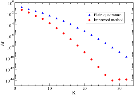
Figure 1: Relative error of free energy as a function of $K$ with $D=32$ on a $1024\times 1024$ lattice. $K$ is the polynomial order of the Gauss-Legendre quadrature in Eq. (8).

3.3 Topological charge density

The expectation value of the topological charge $\langle Q\rangle$ at $\beta=10.0$ is obtained by the numerical derivative of the free energy with respect to $\theta$:

$$\langle Q\rangle=-i\frac{\partial\ln Z}{\partial\theta}.$$ (19)

In Fig. 2 we show the volume dependence of $\langle Q\rangle/V$ around $\theta=\pi$, where the analytic calculation predicts the first order phase transition at any value of $\beta$ u1_anal . We observe that a finite discontinuity emerges with mutual crossings of curves between different volumes at $\theta=\pi$ as the lattice size $L$ is increased. This feature indicates there is a first order phase transition at $\theta=\pi$.

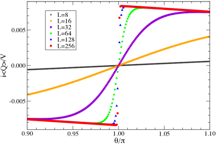
Figure 2: Topological charge density with $8\leq L\leq 256$ as a function of $\theta$ at $\beta=10.0$.

It may be interesting to calculate the topological charge density in the strong coupling limit $\beta=0.0$, whose analytical result was obtained by Seiberg in the infinite volume limit cpn_b0 :

$$\left.\frac{\langle Q\rangle}{V}\right|_{\beta=0}=-i\left(\frac{1}{2}\cot\left(\frac{\theta}{2}\right)-\frac{1}{\theta}\right).$$ (20)

Figure 3 compares the numerical result at $\beta=0.0$ with the analytic expression of Eq. (20). The discrepancy found around $\theta=\pi$ with small lattice size of $L=4$ essentially vanishes once we increase the lattice size up to $L=64$.

Figure 3: Topological charge density with $4\leq L\leq 64$ as a function of $\theta$ at $\beta=0.0$. Solid curve denotes the analytic result of Eq. (20) obtained in the infinite volume limit.

3.4 Topological susceptibility

We investigate the properties of the phase transition by applying the finite size scaling analysis to the topological susceptibility:

$$\chi(L)=-\frac{1}{V}\frac{\partial^{2}\ln Z}{\partial\theta^{2}}.$$ (21)

Figure 4 shows the topological susceptibility as a function of $\theta$ for various lattice sizes. The peak structure is observed and its height $\chi_{\rm max}(L)$ grows as $L$ increases. In order to determine the peak position $\theta_{c}(L)$ and the peak height $\chi_{\rm max}(L)$ at each $L$, we employ the quadratic approximation of the topological susceptibility around the peak position:

$$\chi(L)\sim\chi_{\rm max}(L)+R\left(\theta-\theta_{c}(L)\right)^{2}$$ (22)

with R a constant.

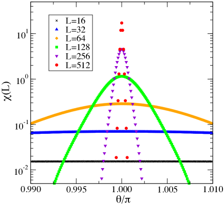
Figure 4: Topological susceptibility $\chi(L)$ as a function of $\theta$ with $16\leq L\leq 512$.

We expect that the peak height scales with $L$ as

$$\chi_{\rm max}(L)\propto L^{\gamma/\nu},$$ (23)

where $\gamma$ and $\nu$ are the critical exponents. The $L$ dependence of the peak height $\chi_{\rm max}(L)$ is plotted in Fig. 5. The solid curve represents the fit result obtained with the fit function of $\chi_{\rm max}(L)=A+BL^{\gamma/\nu}$ choosing the fit range of $128\leq L\leq 1024$. The results for the fit parameters are given by $A=-3(2)\times 10^{-3},B=7.12(8)\times 10^{-5}$ and $\gamma/\nu=1.998(2)$. The value of the exponent $\gamma/\nu=1.998(2)$ is consistent with two, which is the expected critical exponent in the first-order phase transition in the two-dimensional system.

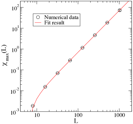
Figure 5: Peak height of topological susceptibility $\chi_{\rm max}(L)$ as a function of $L$. Solid curve denotes the fit result.

4 Summary and outlook

We have applied the TRG method to study the 2D pure U(1) gauge theory with a $\theta$ term. The continuous degrees of freedom are discretized with the Gauss quadrature method. We have confirmed that this model has a first-order phase transition at $\theta=\pi$ as predicted from the analytical calculation. The successful analysis of the model demonstrates an effectiveness of the Gauss quadrature approach to the gauge theories. It should be interesting to apply the TRG-based methods with the Gauss quadrature to higher dimensional gauge theories with $\theta$ term which have been hardly investigated by the Monte Carlo approach because of the sign problem. Another interesting research direction is to include fermionic degrees of freedom following the Grassmann TRG method developed in Ref. schwinger . This is a necessary ingredient toward investigation of the phase structure of QCD at finite density.

- (1) D. J. Gross and E. Witten, Phys. Rev. D21, 446 (1980).
- (2) N. Seiberg, Phys. Rev. Lett. 53, 637 (1984).
- (3) E. Witten, Phys. Rev. Lett. 81, 2862 (1998).
- (4) D. Gaiotto, A. Kapustin, Z. Komargodski, and N. Seiberg, JHEP 1705, 091 (2017).
- (5) M. Levin and C. P. Nave, Phys. Rev. Lett. 99, 120601 (2007).
- (6) Y. Shimizu, Mod. Phys. Lett. A27, 1250035 (2012).
- (7) Y. Shimizu and Y. Kuramashi, Phys. Rev. D90, 014508 (2014).
- (8) Y. Shimizu and Y. Kuramashi, Phys. Rev. D90, 074503 (2014).
- (9) Y. Shimizu and Y. Kuramashi, Phys. Rev. D97, 034502 (2018).
- (10) S. Takeda and Y. Yoshimura, Prog. Theor. Exp. Phys. 2015, 043B01 (2015).
- (11) H. Kawauchi and S. Takeda, Phys. Rev. D93, 114503 (2016).
- (12) D. Kadoh, Y. Kuramashi, Y. Nakamura, R. Sakai, S. Takeda, and Y. Yoshimura, JHEP 1803, 141 (2018).
- (13) R. Sakai, S. Takeda, and Y. Yoshimura, Prog. Theor. Exp. Phys. 2017, 063B07 (2017).
- (14) Y. Yoshimura, Y. Kuramashi, Y. Nakamura, R. Sakai, and S. Takeda, Phys. Rev. D97, 054511 (2018).
- (15) J. Unmuth-Yockey, J. Zhang, A. Bazavov, Y. Meurice, and S.-W. Tsai, Phys. Rev. D98, 094511 (2018).
- (16) D. Kadoh, Y. Kuramashi, Y. Nakamura, R. Sakai, S. Takeda, and Y. Yoshimura, JHEP 1905, 184 (2019).
- (17) Y. Kuramashi and Y. Yoshimura, JHEP 1908, 023 (2019).
- (18) N. Butt, S. Catterall, Y. Meurice, and J. Unmuth-Yockey, arXiv:1911.01285 [hep-lat].
- (19) D. Kadoh, Y. Kuramashi, Y. Nakamura, R. Sakai, S. Takeda, and Y. Yoshimura, JHEP 2002, 161 (2020).
- (20) S. R. Coleman, Ann. Phys. (N.Y.) 101, 239 (1976).
- (21) L. Funcke, K. Jansen, and S. Kühn, arXiv:1908.00551 [hep-lat] and references therein.
- (22) U.-J. Wiese, Nucl. Phys. B318, 153 (1989).
- (23) Y. Liu, Y. Meurice, M. P. Qin, J. Unmuth-Yockey, T. Xiang, Z. Y. Xie, J. F. Yu, and H. Zou, Phys. Rev. D88, 056005 (2013).
- (24) A. S. Hassan, M. Imachi, and H. Yoneyama, Prog. Theor. Phys. 93, 161 (1995).
- (25) A. S. Hassan, M. Imachi, N. Tsuzuki, and H. Yoneyama, Prog. Theor. Phys. 94, 861 (1995).
- (26) J. C. Plefka and S. Samuel, Phys. Rev. D56, 44 (1997).