Measurement Error Correction in Particle Tracking Microrheology

Abstract

In diverse biological applications, particle tracking of passive microscopic species has become the experimental measurement of choice – when either the materials are of limited volume, or so soft as to deform uncontrollably when manipulated by traditional instruments. In a wide range of particle tracking experiments, a ubiquitous finding is that the mean squared displacement (MSD) of particle positions exhibits a power-law signature, the parameters of which reveal valuable information about the viscous and elastic properties of various biomaterials. However, MSD measurements are typically contaminated by complex and interacting sources of instrumental noise. As these often affect the high-frequency bandwidth to which MSD estimates are particularly sensitive, inadequate error correction can lead to severe bias in power law estimation and thereby, the inferred viscoelastic properties. In this article, we propose a novel strategy to filter high-frequency noise from particle tracking measurements. Our filters are shown theoretically to cover a broad spectrum of high-frequency noises, and lead to a parametric estimator of MSD power-law coefficients for which an efficient computational implementation is presented. Based on numerous analyses of experimental and simulated data, results suggest our methods perform very well compared to other denoising procedures.

Keywords Particle tracking  $\cdot$ Subdiffusion  $\cdot$ Measurement error  $\cdot$ High-frequency filtering

1 Introduction

With the development of high-resolution microscopy, single-particle tracking has emerged as an invaluable tool in the study of biophysical and transport properties of diverse soft materials (e.g., Mason et al., 1997). Examples of applications include cellular membrane dynamics (Saxton and Jacobson, 1997), drug delivery mechanisms (Suh et al., 2005), properties of colloidal particles (Lee et al., 2007), mechanisms of virus infection (van der Schaar et al., 2008), microrheology of complex fluids and living cells (Mason et al., 1997; Wirtz, 2009) and functional analyses of the cytoskeleton (Gal et al., 2013).

Passive single-particle tracking refers to experiments in which microscale probes and/or pathogens (e.g., viruses) are recorded without external forcing, producing high-resolution time series of particle positions from which dynamical properties of the transport medium are inferred. In many of these experiments, the resulting analysis hinges pivotally on the measurement of particles’ mean square displacement (MSD), which for a $k$-dimensional particle trajectory $\bm{X}(t)=\bigl{(}X_{1}(t),\ldots,X_{k}(t)\bigl{)}$ (with $k\in\{1,2,3\}$ depending on the experiment) is given by

$$\operatorname{\textsc{msd}}_{\bm{X}}(t)=\frac{1}{k}\times E\bigl{[}\lVert\bm{X}(t)-\bm{X}(0)\rVert^{2}\bigr{]}=\frac{1}{k}\times\sum_{j=1}^{k}E\bigl{[}\lvert X_{j}(t)-X_{j}(0)\rvert^{2}\bigr{]}.$$ (1.1)

For particles diffusing in viscous media (e.g., water, glycerol), the position time series are accurately modeled by Brownian motion. The MSD is then linear in time,

$$\operatorname{\textsc{msd}}_{\bm{X}}(t)=2Dt,$$ (1.2)

and the diffusion coefficient $D$ is determined by the Stokes-Einstein relation (Einstein, 1956; Edward, 1970)

$$D=\frac{k_{B}T}{6\pi\eta r},$$ (1.3)

where $r$ is the particle radius, $T$ is temperature, $\eta$ is the viscosity of the medium, and $k_{B}$ is the Boltzmann’s constant. However, due to the microstructure of large molecular weight biopolymers (e.g., mucins in mucosal layers), most biological fluids are viscoelastic. In such fluids, a nearly ubiquitous experimental finding has been that the MSD has sublinear power-law scaling over a given range of timescales,

$$\operatorname{\textsc{msd}}_{\bm{X}}(t)\sim 2Dt^{\alpha},\qquad t_{\textnormal{min}}<t<t_{\textnormal{max}},\quad 0<\alpha<1.$$ (1.4)

This phenomenon is referred to as subdiffusion. Due to its pervasiveness, interpretation of the subdiffusion parameters $(\alpha,D)$ has far-reaching consequences for numerous biological applications, for example: distinguishing signatures of healthy versus pathological human bronchial epithelial mucus (Hill et al., 2014a); cytoplasmic crowding (Weiss et al., 2004); local viscoelasticity in protein networks (Amblard et al., 1996); dynamics of telomeres in the nucleus of mammalian cells (Bronstein et al., 2009); and microstructure dynamics of entangled F-Actin networks (Wong et al., 2004).

Unlike viscous fluids exhibiting ordinary (linear) diffusion, the precise manner in which the properties of a viscoelastic fluid determine its subdiffusion parameters $(\alpha,D)$ is unknown, such that $(\alpha,D)$ must be estimated from particle-tracking data. To this end, a widely-used approach is to apply ordinary least-squares to a nonparametric estimate of the MSD (e.g., Qian et al., 1991). While minimal modeling assumptions suffice to make this subdiffusion estimator consistent (Michalet, 2010), for finite-length trajectories, the nonparametric MSD estimator at longer timescales is severely biased (Mellnik et al., 2016). Therefore, in practice a good portion of the MSD must be discarded, at the expense of considerable loss in statistical efficiency. In contrast, fully parametric subdiffusion estimators specify a complete stochastic process for $\bm{X}(t)$ as a function of $(\alpha,D)$ (e.g., Berglund, 2010; Lysy et al., 2016; Mellnik et al., 2016), whereby optimal statistical efficiency is achieved via likelihood inference. However, the accuracy of these parametric estimators critically depends on the adequacy of the parametric model, and particle tracking measurements are well known to be corrupted by various sources of experimental noise.

Noise in single-particle tracking experiments can be categorized roughly into two types. Low-frequency noise, originating primarily from slow drift currents in the fluid itself, is typically removed from particle trajectories by way of various linear detrending methods (e.g., Fong et al., 2013; Rowlands and So, 2013; Koslover et al., 2016; Mellnik et al., 2016). In contrast, high-frequency noise can be due to a variety of reasons: mechanical vibrations of the instrumental setup; particle displacement while the camera shutter is open; noisy estimation of true position from the pixelated microscopy image; error-prone tracking of particle positions when they are out of the camera focal plane. A systematic review of high-frequency or localization errors in single-particle tracking is given by Deschout et al. (2014). The effect of such noise is to distort the MSD at the shortest observation timescales. Since fully-parametric models extract far more information about $(\alpha,D)$ from short timescales than long ones, their accuracy in the presence of high-frequency noise can suffer considerably.

In a seminal work, Savin and Doyle (2005) present a theoretical model for localization error, encompassing most of the approaches reviewed by Deschout et al. (2014). The parameters of the Savin-Doyle model can be derived either from first-principles (for instance, by analyzing uncertainty in position-extraction algorithms, e.g., Mortensen et al., 2010; Chenouard et al., 2014; Kowalczyk et al., 2014; Burov et al., 2017), or empirically (via signal-free control experiments, e.g., Savin and Doyle, 2005; Deschout et al., 2014). Model-based methods for estimating localization error have also been proposed, under the assumption of ordinary diffusion $\alpha=1$ (e.g., Michalet, 2010; Berglund, 2010; Michalet and Berglund, 2012; Vestergaard et al., 2014; Ashley and Andersson, 2015; Calderon, 2016).

The Savin-Doyle theoretical framework accounts for a wide range of experimental errors. However, due to the extreme complexity and inter-dependence between various sources of localization error, the Savin-Doyle model cannot account for them all. This is illustrated in the control experiment of Figure 1, where trajectories of $1\text{\,}\mathrm{\SIUnitSymbolMicro m}$ diameter tracer particles are recorded in water, for which it is known that $\alpha=1$ and for which $D$ may be determined theoretically by the Stokes-Einstein relation (1.3). However, the Savin-Doyle model estimates both of these parameters with considerable bias (Figure 1).

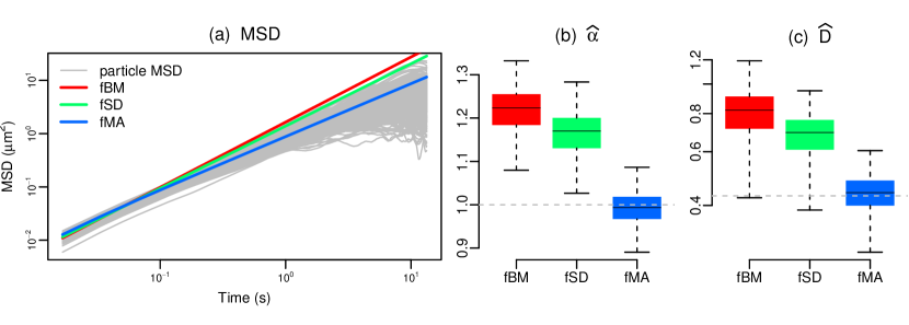
Figure 1: (a) Pathwise empirical MSD for $1931$ particles of diameter $1\text{\,}\mathrm{\SIUnitSymbolMicro m}$ recorded in water at $\Delta t=$1\text{/}60\text{\,}\mathrm{s}$$ for a duration of $30\text{\,}\mathrm{s}$ ($N=1800$ observations). Straight lines correspond to fitted MSDs for three parametric models: fractional Brownian Motion (fBM), fBM with Savin-Doyle noise correction (fSD), and fBM with one of the noise correction models proposed in this paper (fMA). (b-c) Estimated values of $\alpha$ and $D$ for each particle and parametric model. The predicted values from Stokes-Einstein theory are given by the horizontal dashed lines.

In this article, we propose a likelihood-based filtering method to correct for localization errors, complementing the theoretical Savin-Doyle approach. Our filters can be readily applied to any parametric model of particle dynamics, and are demonstrated theoretically to cover a very broad spectrum of high-frequency noises. We show how to combine our filters with parametric methods of low-frequency drift correction, and estimate all parameters of both subdiffusion and noise models in a computationally efficient manner. Extensive simulations and analyses of experimental data suggest that our filters perform remarkably well, both for estimating the true values of $(\alpha,D)$, and compared to state-of-the-art high-frequency denoising procedures (e.g., Figure 1).

The remainder of the article is organized as follows. In Section 2 we review a number of existing subdiffusion estimators and high-frequency error-correction techniques. In Section 3 we present our family of high-frequency filters, with theoretical justification for the proposed construction. Sections 4 and 5 contain analyses of numerous simulated and real particle-tracking experiments comparing our proposed subdiffusion estimators to existing alternatives. Section 6 offers concluding remarks and directions for future work.

2 Existing Subdiffusion Estimators

2.1 Semiparametric Least-Squares Estimator

Let $\bm{X}=(\bm{X}_{0},\ldots,\bm{X}_{N})$, $\bm{X}_{n}=\bm{X}(n\cdot\Delta t)$, denote the discrete-time observations of a given particle trajectory $\bm{X}(t)$ recorded at frequency $1/\Delta t$. Assuming that $\bm{X}(t)$ has second-order stationary increments,

$$E\bigl{[}\lVert\bm{X}(s+t)-\bm{X}(s)\rVert^{2}\bigr{]}=E\bigl{[}\lVert\bm{X}(t)-\bm{X}(0)\rVert^{2}\bigr{]},$$ (2.1)

a standard nonparametric estimator for the particle MSD is given by

$$\widehat{\operatorname{\textsc{msd}}}_{\bm{X}}(n\cdot\Delta t)=\frac{1}{k\cdot(N-n+1)}\sum_{i=0}^{N-n}\lVert\bm{X}_{n+i}-\bm{X}_{i}\rVert^{2}.$$ (2.2)

Based on the linear relation

$$\log\operatorname{\textsc{msd}}_{\bm{X}}(t)=\log 2D+\alpha\log t$$ (2.3)

over the subdiffusion timescale $t\in(t_{\textnormal{min}},t_{\textnormal{max}})$, a commonly-used subdiffusion estimator (e.g., Gal et al., 2013) is obtained from the least-squares regression of $y_{n}=\log\bigl{(}\widehat{\operatorname{\textsc{msd}}}_{\bm{X}}(n\cdot\Delta t)\bigr{)}$ onto $x_{n}=\log(n\cdot\Delta t)$, namely

$$\hat{\alpha}=\frac{\sum_{n=0}^{N}(y_{n}-\bar{y})(x_{n}-\bar{x})}{\sum_{n=0}^{N}(x_{n}-\bar{x})^{2}},\qquad\hat{D}=\tfrac{1}{2}\exp(\bar{y}-\hat{\alpha}\bar{x}).$$ (2.4)

The least-squares subdiffusion estimator (2.4) is easy to implement, and it is consistent under the minimal assumption of (2.1) and when the power-law scaling (1.4) holds for all $t>t_{\textnormal{min}}$ (Sikora et al., 2017). However, the least-squares estimator also presents two major drawbacks. First, the errors underlying the regression (2.3) are neither homoscedastic nor uncorrelated (Sikora et al., 2017), such that (2.4) is statistically inefficient. Second, it is common practice to account for low-frequency noise by calculating the empirical MSD (2.2) from the drift-subtracted positions

$$\tilde{\bm{X}}_{n}=(\bm{X}_{n}-\bm{X}_{0})-n\cdot\overline{\Delta\bm{X}},$$ (2.5)

where $\overline{\Delta\bm{X}}=\frac{1}{N}\sum_{n=1}^{N}(\bm{X}_{n}-\bm{X}_{n-1})$ is the average displacement over the interobservation time $\Delta t$. However, a straightforward calculation (Mellnik et al., 2016) shows that $\tilde{\bm{X}}_{N}=0$, such that $\widehat{\operatorname{\textsc{msd}}}_{X}(n\cdot\Delta t)$ becomes increasingly biased towards zero as $n$ approaches $N$. Consequently, a widely-reported figure (e.g., Weihs et al., 2007) suggests that, prior to fitting (2.4), the largest 30% of MSD lag times are discarded, thus severely compounding the inefficiency of the least-squares subdiffusion estimator when low-frequency noise correction is applied.

2.2 Fully-Parametric Subdiffusion Estimators

While the semiparametric estimator (2.4) operates under minimal modeling assumptions, complete specification of the stochastic process $\bm{X}(t)$ provides not only a considerable increase in statistical efficiency (e.g., Mellnik et al., 2016), but in fact is necessary to establish dynamical properties of particle-fluid interactions which cannot be determined from second-order moments (such as the MSD) alone (Gal et al., 2013; Lysy et al., 2016). A convenient framework for stochastic subdiffusion modeling is the location-scale model of Lysy et al. (2016),

$$\bm{X}(t)=\sum_{j=1}^{d}\bm{\beta}_{j}f_{j}(t)+\bm{\Sigma}^{1/2}\bm{Z}(t),$$ (2.6)

where $f_{1}(t),\ldots f_{d}(t)$ are known functions accounting for low-frequency drift (typically linear, $f_{1}(t)=t$, and occasionally quadratic, $f_{2}(t)=t^{2}$), $\bm{\beta}_{1},\ldots,\bm{\beta}_{d}\in\mathbb{R}^{k}$ are regression coefficients, $\bm{\Sigma}_{k\times k}$ is a variance matrix, and $\bm{Z}(t)=\bigl{(}Z_{1}(t),\ldots,Z_{k}(t)\bigr{)}$ are iid continuous stationary-increments (CSI) Gaussian processes with mean zero and MSD parametrized by ${\bm{\varphi}}$,

$$\operatorname{\textsc{msd}}_{Z}(t)=E\bigl{[}\lVert Z_{j}(t)-Z_{j}(0)\rVert^{2}\bigr{]}=\eta(t\mid{\bm{\varphi}}),$$ (2.7)

such that the MSD of the drift-subtracted process $\tilde{\bm{X}}(t)=\bm{X}(t)-\sum_{j=1}^{d}\bm{\beta}_{j}f_{j}(t)$ is given by

$$\operatorname{\textsc{msd}}_{\tilde{\bm{X}}}(t)=\tfrac{1}{k}\operatorname{tr}(\bm{\Sigma})\cdot\eta(t\mid{\bm{\varphi}}).$$ (2.8)

Perhaps the simplest parametric subdiffusion model sets $Z_{j}(t)=B_{\alpha}(t)$ to be fractional Brownian Motion (fBM) (e.g., Szymanski and Weiss, 2009; Weiss, 2013), a mean-zero CSI Gaussian process with covariance function

$$\operatorname{cov}\bigl{(}B_{\alpha}(t),B_{\alpha}(s)\bigr{)}=\tfrac{1}{2}(|t|^{\alpha}+|s|^{\alpha}-|t-s|^{\alpha}),\qquad 0<\alpha<2.$$ (2.9)

Indeed, as the covariance function of a CSI process is completely determined by its MSD, fBM is the only (mean-zero) CSI Gaussian process exhibiting uniform subdiffusion,

$$\operatorname{\textsc{msd}}_{B_{\alpha}}(t)=t^{\alpha},\qquad 0<t<\infty,$$ (2.10)

in which case the diffusivity coefficient is given by

$$D=\frac{1}{2k}\times\operatorname{tr}(\bm{\Sigma}).$$

Other examples of driving CSI processes are the confined diffusion model of Ernst et al. (2017) and the viscoelastic Generalized Langevin Equation (GLE) of McKinley et al. (2009), both of which exhibit transient subdiffusion, i.e., power-law scaling only on a given timescale $t\in(t_{\textnormal{min}},t_{\textnormal{max}})$. In this case, the subdiffusion parameters $(\alpha,D)$ become functions of the other parameters, namely $\alpha=\alpha({\bm{\varphi}})$ and $D=D({\bm{\varphi}},\bm{\Sigma})$. We shall revisit these transient subdiffusion models in Section 4.

Parameter estimation for the location-scale model (2.6) can be done by maximum likelihood. Let $\Delta\bm{X}_{n}=\bm{X}_{n+1}-\bm{X}_{n}$ denote the $n$th trajectory increment, and $\Delta\bm{X}=(\Delta\bm{X}_{0},\ldots,\Delta\bm{X}_{N-1})$. Then $\Delta\bm{X}$ are consecutive observations of a stationary Gaussian time series with autocorrelation function

$$\operatorname{\textsc{acf}}_{\Delta\bm{X}}(h)=\operatorname{cov}(\Delta\bm{X}_{n},\Delta\bm{X}_{n+h})=\bm{\Sigma}\times\gamma(h\mid{\bm{\varphi}}),$$

where

$$\gamma(n\mid{\bm{\varphi}})=\tfrac{1}{2}\times\Bigl{\{}\eta(|n-1|\cdot\Delta t\mid{\bm{\varphi}})+\eta(|n+1|\cdot\Delta t\mid{\bm{\varphi}})-2\eta(|n|\cdot\Delta t\mid{\bm{\varphi}})\Bigr{\}},$$

such that the increments follow a matrix-normal distribution (defined in Appendix A),

$$\Delta\bm{X}_{N\times k}\sim\textnormal{MatNorm}(\bm{F}\bm{\beta},\bm{V}_{\bm{\varphi}},\bm{\Sigma}),$$ (2.11)

where $\bm{\beta}_{d\times k}=[\bm{\beta}_{1}\mid\cdots\mid\bm{\beta}_{d}]^{\prime}$, $\bm{F}_{N\times d}$ is a matrix with elements $F_{nm}=f_{m}((n+1)\cdot\Delta t)-f_{m}(n\cdot\Delta t)$, and $\bm{V}_{\bm{\varphi}}$ is an $N\times N$ Toeplitz matrix with element $(n,m)$ given by $V_{\bm{\varphi}}^{(n,m)}=\gamma(n-m\mid{\bm{\varphi}})$, such that the log-likelihood function is given by

$$\begin{split}\ell({\bm{\varphi}},\bm{\beta},\bm{\Sigma}\mid\Delta\bm{X})=&-\frac{1}{2}\operatorname{tr}\left\{\bm{\Sigma}^{-1}(\Delta\bm{X}-\bm{F}\bm{\beta})^{\prime}\bm{V}_{{\bm{\varphi}}}^{-1}(\Delta\bm{X}-\bm{F}\bm{\beta})\right\}\\ &-\frac{N}{2}\log|\bm{\Sigma}|-\frac{k}{2}\log|\bm{V}_{{\bm{\varphi}}}|.\end{split}$$ (2.12)

In order to calculate the MLE of $\bm{\theta}=({\bm{\varphi}},\bm{\beta},\bm{\Sigma})$, model (2.6) has two appealing properties. First, for given ${\bm{\varphi}}$, the conditional MLEs of $\bm{\beta}$ and $\bm{\Sigma}$ can be obtained analytically as shown in Appendix A, such that the optimization problem can be reduced by $2k+{k\choose 2}$ dimensions by calculating the profile likelihood $\ell_{\textnormal{prof}}({\bm{\varphi}}\mid\Delta\bm{X})=\max_{\bm{\beta},\bm{\Sigma}}\ell({\bm{\varphi}},\bm{\beta},\bm{\Sigma}\mid\Delta\bm{X})$. Second, we show in Appendix A that the computational bottleneck in $\ell_{\textnormal{prof}}({\bm{\varphi}}\mid\Delta\bm{X})$ involves the calculation of $\bm{V}_{{\bm{\varphi}}}^{-1}$ and its log-determinant. While the computational cost of these operations is $\mathcal{O}(N^{3})$ for general variance matrices, for Toeplitz matrices it is only $\mathcal{O}(N^{2})$ using the Durbin-Levinson algorithm (Levinson, 1947; Durbin, 1960), or more recently, only $\mathcal{O}(N\log^{2}N)$ using the Generalized Schur algorithm (Kailath et al., 1979; Ammar and Gragg, 1988; Ling and Lysy, 2017).

2.3 Savin-Doyle Noise Model

In order to characterize high-frequency noise in particle tracking experiments, Savin and Doyle (2005) decompose it into so-called static and dynamic sources. Static noise is due to measurement error in the recording of the position of the particle at a given time. Thus, if $\bm{X}_{n}$ denotes the true particle position at time $t=n\cdot\Delta t$, and $\bm{Y}_{n}$ is its recorded value, then Savin and Doyle suggest the additive error model

$$\bm{Y}_{n}=\bm{X}_{n}+\bm{\varepsilon}_{n},$$ (2.13)

where $\bm{\varepsilon}_{n}$ is a $k$-dimensional stationary process independent of $\bm{X}(t)$. Thus, if the autocorrelation of the static noise is denoted as

$$\operatorname{\textsc{acf}}_{\bm{\varepsilon}}(n)=\operatorname{cov}(\bm{\varepsilon}_{m},\bm{\varepsilon}_{m+n}),$$ (2.14)

the MSD of the observations becomes

$$\operatorname{\textsc{msd}}_{\bm{Y}}(n) =\tfrac{1}{k}\times E\bigl{[}\lVert\bm{Y}_{n}-\bm{Y}_{0}\rVert^{2}\bigr{]}$$ (2.15)

$$=\operatorname{\textsc{msd}}_{\bm{X}}(n)+\tfrac{1}{k}\times 2\cdot\operatorname{tr}\bigl{(}\operatorname{\textsc{acf}}_{\bm{\varepsilon}}(0)-\operatorname{\textsc{acf}}_{\bm{\varepsilon}}(n)\bigr{)}.$$

Savin and Doyle describe how to estimate the temporal dynamics of $\bm{\varepsilon}_{n}$ by recording immobilized particles, i.e., for which it is known that $\bm{X}_{n}\equiv 0$. Over a wide range of signal-to-noise ratios, they report that $\bm{\varepsilon}_{n}$ is effectively white noise,

$$\operatorname{\textsc{acf}}_{\bm{\varepsilon}}(n)=\bm{\Sigma}_{\varepsilon}\cdot\mathfrak{1}(n=0),$$

a result corroborated by many other experiments (for example, see references in Deschout et al., 2014, Figure 2). For the canonical trajectory model of fractional Brownian motion, $\operatorname{\textsc{msd}}_{\bm{X}}(t)=2Dt^{\alpha}$, white static noise has the effect of raising the MSD at the shortest timescales, as seen in Figure 2.

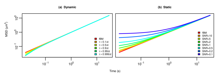
Figure 2: Effect of localization error on the MSD of an fBM process $X(t)=B^{\alpha}_{t}$ with $\alpha=0.8$ and $\Delta t=1/60$. (a) Dynamic error, as a function of exposure time $\tau$. (b) Static error, as a function of the signal-to-noise ratio, $\textnormal{SNR}=\operatorname{var}(\Delta B^{\alpha}_{n})/\operatorname{var}(\varepsilon_{n})$.

In contrast to static noise, Savin and Doyle define dynamic noise as originating from movement of the particle during the camera frame exposure time. Thus, if the camera exposure time is $\tau<\Delta t$ (as it must be less than the framerate), the recorded position of the particle at time $t=n\cdot\Delta t$ is

$$\bm{Y}_{n}=\frac{1}{\tau}\int_{0}^{\tau}\bm{X}(n\cdot\Delta t-s)\mathop{}\!\mathrm{d}s.$$ (2.16)

The dynamic-error MSD for an fBM process $X(t)=B^{\alpha}_{t}$ is given in Appendix B. Larger values of $\tau$ have the effect of lowering the MSD at the shortest timescales, as seen in Figure 2.

Combining static and dynamic models, the Savin-Doyle localization error model is

$$\bm{Y}_{n}=\frac{1}{\tau}\int_{0}^{\tau}\bm{X}(n\cdot\Delta t-s)\mathop{}\!\mathrm{d}s+\bm{\varepsilon}_{n}.$$ (2.17)

When $\bm{X}(t)=\sum_{m=1}^{d}\bm{\beta}_{m}f_{m}(t)+\bm{\Sigma}^{1/2}\bm{Z}(t)$ follows the location-scale model (2.6), and the static noise has the simplified form $\bm{\Sigma}_{\varepsilon}=\sigma^{2}\cdot\bm{\Sigma}$, parametric inference can be conducted using the computationally efficient methods of Section 2.2. Explicit calculations for the fBM process with $\operatorname{\textsc{msd}}_{Z}(t)=t^{\alpha}$ are given in Appendix B.

Thus, the fBM + Savin-Doyle (fSD) model has three MSD parameters: ${\bm{\varphi}}=(\alpha,\tau,\sigma)$. Its maximum likelihood estimates of the subdiffusion parameters $(\alpha,D)$ are $\hat{\alpha}$ and $\hat{D}=(1/2k)\cdot\operatorname{tr}(\hat{\bm{\Sigma}})$. While these estimates successfully correct for many types of high-frequency measurement errors, the fSD model has two important limitations. First, Figure 2 shows that the Savin-Doyle model has little ability to correct negatively biased MSDs at the shortest timescales. Indeed, the camera aperture time $\tau$ is typically at least an order of magnitude smaller than $\Delta t$, in which case the effect of the dynamic error in Figure 2 is extremely small, and insufficient to explain larger negative MSD biases as in Figure 1. Second, the Savin-Doyle model uses one parameter ($\tau$) to lower the MSD, and a different parameter ($\sigma$) to raise it. This leads to an identifiability issue which adversely affects the subdiffusion estimator, as we shall see in Section 4. Complementing the theoretically derived Savin-Doyle approach, we present a general high-frequency noise filtering framework in the following section.

3 Proposed Method

In order to formulate our proposed method of filtering the localization errors in single particle tracking experiments, we begin with the following definition of high frequency noise. Let us first focus on a one-dimensional zero-drift CSI process $X(t)$ with $E[X(t)]=0$, and let $\bm{\mathcal{X}}=\{X_{n}:n\geq 0\}$ and $\bm{\mathcal{Y}}=\{Y_{n}:n\geq 0\}$ denote the true and recorded particle position process at times $t=n\cdot\Delta t$. Then we shall say that the observation process $\bm{\mathcal{Y}}$ contains only high frequency noise if the low-frequency second-order dynamics of the true and recorded particle positions are the same, namely

$$\lim_{n\rightarrow\infty}\frac{\operatorname{\textsc{msd}}_{Y}(n)}{\operatorname{\textsc{msd}}_{X}(n)}=1.$$ (3.1)

Given the true position process $\bm{\mathcal{X}}$, our noise model sets the observed position process to be of autoregressive/moving-average $\operatorname{ARMA}(p,q)$ type:

$$Y_{n}=\sum_{i=1}^{p}\theta_{i}Y_{n-i}+\sum_{j=0}^{q}\rho_{j}X_{n-j},\qquad n\geq r=\max\{p,q\}.$$ (3.2)

For $0\leq n<r$, $Y_{n}$ is defined via the stationary increment process $\Delta\bm{\mathcal{X}}=\{\Delta X_{n}:n\in\mathbb{Z}\}$. That is, with the usual parameter restrictions

$$\min_{\{z\in\mathbb{C}:|z|\leq 1\}}{\textstyle\big{|}1-\sum_{i=1}^{p}\theta_{i}z^{i}\big{|}}>0,\qquad\min_{\{z\in\mathbb{C}:|z|\leq 1\}}{\textstyle\big{|}\rho_{0}-\sum_{j=1}^{q}\rho_{j}z^{j}\big{|}}>0,$$ (3.3)

(e.g. Brockwell and Davis, 1991), the increment process $\Delta\bm{\mathcal{Y}}=\{\Delta Y_{n}:n\in\mathbb{Z}\}$ defined by

$$\Delta Y_{n}=\sum_{i=1}^{p}\theta_{i}\Delta Y_{n-i}+\sum_{j=0}^{q}\rho_{j}\Delta X_{n-j}$$ (3.4)

is a well-defined stationary process which can be causally derived from $\Delta\bm{\mathcal{X}}$, and vice-versa. Moreover, setting $Y_{n}=\sum_{i=0}^{n-1}\Delta Y_{i}$ obtains the ARMA relation (3.2) on the position scale for $n\geq r$.

One may note in model (3.2) that $\bm{\rho}=(\rho_{0},\ldots,\rho_{q})$ and $\operatorname{var}(\Delta X_{n})$ cannot be identified simultaneously. This issue is typically resolved in the time-series literature by imposing the restriction $\rho_{0}=1$. However, in order for the recorded positions to adhere to a high-frequency error model as defined by (3.1), a different restriction must be imposed:

Theorem 1.

Let $\bm{\mathcal{X}}$ and $\bm{\mathcal{Y}}$ denote the true and recorded position processes, with the latter defined by an $\operatorname{ARMA}(p,q)$ representation of the former as in (3.4). Then $\bm{\mathcal{Y}}$ is a high-frequency error model for $\bm{\mathcal{X}}$ as defined by (3.1) if and only if

$$\rho_{0}=1-\sum_{i=1}^{p}\theta_{i}-\sum_{j=1}^{q}\rho_{j}.$$ (3.5)

The proof is given in Appendix C.3. Indeed, the following result (proved in Appendix C.4) shows that the family of $\operatorname{ARMA}(p,q)$ noise models (3.2) is sufficient to describe any high-frequency noise model to arbitrary accuracy:

Theorem 2.

Let $\bm{\mathcal{Y}}$ be a stochastic process of recorded positions defined as a high-frequency noise model via (3.1). If $\bm{\mathcal{Y}}$ satisfies the assumptions in Appendix C.4, then for any $\epsilon>0$ we may find an $\operatorname{ARMA}(p,q)$ noise model $\bm{\mathcal{Y}^{\star}}=\{Y^{\star}_{n}:n\geq 0\}$ satisfying (3.2) such that for all $n\geq 0$ we have

$$\left|\frac{\operatorname{\textsc{msd}}_{Y^{\star}}(n)}{\operatorname{\textsc{msd}}_{Y}(n)}-1\right|<\epsilon.$$ (3.6)

3.1 Efficient Computations for the Location-Scale Model

Let us now consider a $k$-dimensional position process $\bm{X}(t)=\sum_{j=1}^{d}\bm{\beta}_{j}f_{j}(t)+\bm{\Sigma}^{1/2}\bm{Z}(t)$ following the location-scale model (2.6). Then we may construct an $\operatorname{ARMA}(p,q)$ high-frequency model for the measured positions as follows. Starting from the drift-free stationary increment process $\Delta\tilde{\bm{\mathcal{X}}}=\{\Delta\tilde{\bm{X}}_{n}=\bm{\Sigma}^{1/2}\Delta\bm{Z}_{n}:n\in\mathbb{Z}\}$, define the increment process $\Delta\tilde{\bm{\mathcal{Y}}}=\{\Delta\bm{Y}_{n}:n\in\mathbb{Z}\}$ via

$$\Delta\tilde{\bm{Y}}_{n}=\sum_{i=1}^{p}\theta_{i}\Delta\tilde{\bm{Y}}_{n-i}+\sum_{j=0}^{q}\rho_{j}\Delta\tilde{\bm{X}}_{n-j}.$$ (3.7)

Then under parameter restrictions (3.3), $\Delta\tilde{\bm{\mathcal{Y}}}$ is a well-defined stationary process with $E[\Delta\tilde{\bm{Y}}_{n}]=\bm{0}$. In order to add drift to the high-frequency noise model (3.7), let

$$\Delta\bm{X}_{n} =\begin{cases}\Delta\tilde{\bm{X}}_{n},&n<0,\\ \Delta\tilde{\bm{X}}_{n}+\sum_{m=1}^{d}\bm{\beta}_{j}\Delta f_{nj},&n\geq 0,\end{cases}$$ (3.8)

$$\Delta\bm{Y}_{n} =\begin{cases}\Delta\tilde{\bm{Y}}_{n},&n<0\\ \sum_{i=1}^{p}\theta_{i}\Delta\bm{Y}_{n-i}+\sum_{j=0}^{q}\rho_{j}\Delta\bm{X}_{n-j},&n\geq 0,\end{cases}$$

where $\Delta f_{nj}=f_{j}((n+1)\cdot\Delta t)-f_{m}(n\cdot\Delta t)$. Then for $n\geq 0$, $\bm{X}_{n}=\sum_{i=0}^{n-1}\Delta\bm{X}_{i}$ corresponds to discrete-time observations of $\bm{X}(t)$ from the location-scale model (2.6), and $\bm{Y}_{n}=\sum_{i=0}^{n-1}\Delta\bm{Y}_{i}$ satisfies the $\operatorname{ARMA}(p,q)$ relation (3.2). Moreover, the observed increments $\Delta\bm{Y}=(\Delta\bm{Y}_{0},\ldots,\Delta\bm{Y}_{N-1})$ follow a matrix-normal distribution

$$\Delta\bm{Y}\sim\textnormal{MatNorm}(\bm{F}_{\bm{\varphi}}\bm{\beta},\bm{V}_{\bm{\varphi}},\bm{\Sigma}),$$

where $\bm{F}_{\bm{\varphi}}$ is an $N\times k$ matrix with elements

$$F_{nm}=-\sum_{i=1}^{\min\{n,p\}}\theta_{i}F_{n-i,m}+\sum_{j=0}^{\min\{n,q\}}\rho_{j}\Delta f_{n-j,m},$$ (3.9)

and $\bm{V}_{\bm{\varphi}}$ is an $N\times N$ Toeplitz matrix with element $(n,m)$ given by $V_{\bm{\varphi}}^{(n,m)}=\operatorname{\textsc{acf}}_{\Delta Y}(|n-m|)$. Thus, we may use the computationally efficient methods of Section 2.2 for parameter inference, given the autocorrelation function $\operatorname{\textsc{acf}}_{\Delta Y}(n)$ defined by (3.4). For pure moving-average processes ($p=0$), this function is available in closed-form given an arbitrary true increment autocorrelation function $\operatorname{\textsc{acf}}_{\Delta Z}(n)$. For $p>0$, an accurate and computationally efficient approximation is provided in Appendix C.2.

3.2 The Fractional $\operatorname{MA}(1)$ Noise Model

Perhaps the simplest $\operatorname{ARMA}(p,q)$ noise model is that with $p=0$ and $q=1$, i.e., the first-order moving-average $\operatorname{MA}(1)$ model given by

$$\bm{Y}_{n}=(1-\rho)\bm{X}_{n}+\rho\bm{X}_{n-1},$$ (3.10)

where $|\rho|<1$ is required to satisfy (3.3), and $\rho<\tfrac{1}{2}$ is required to satisfy (3.1). The autocorrelation of the observed increments becomes

$$\operatorname{\textsc{acf}}_{\Delta\bm{Y}}(n)=\operatorname{\textsc{acf}}_{\Delta\bm{X}}(n)+(1-\rho)\rho\big{[}\operatorname{\textsc{acf}}_{\Delta\bm{X}}(|n-1|)+\operatorname{\textsc{acf}}_{\Delta\bm{X}}(n+1)-2\operatorname{\textsc{acf}}_{\Delta\bm{X}}(n)\big{]},$$ (3.11)

where $\operatorname{\textsc{acf}}_{\Delta\bm{X}}(n)$ is the autocorrelation of the true increment process. Of particular interest is when $\bm{X}(t)$ is fractional Brownian motion, for which we refer to the corresponding $\operatorname{MA}(1)$ noise model as fMA. The MSD of such a model is plotted in Figure 3 for a range of values $\rho\in(-1,\tfrac{1}{2})$. As with the fractional Savin-Doyle (fSD) model (2.17), $\rho>0$ raises the high-frequency correlations in the observation process, whereas $\rho<0$ lowers them. A similar MSD plot for the fSD model is given in Figure 3. While both high-frequency noise models can similarly raise the MSD at short timescales, the fMA model has much higher capacity to lower it.

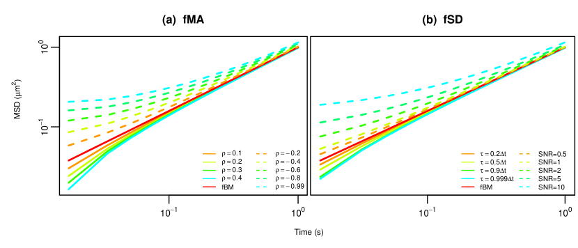
Figure 3: (a) MSD of the fMA model with $\alpha=0.8$ and different values of $\rho$. (b) MSD of the fSD model with $\alpha=0.8$ and different values of $\tau$ and signal-to-noise ratio $\textnormal{SNR}=\operatorname{var}(\Delta B^{\alpha})/\sigma^{2}$.

In order to examine this difference more carefully, the following experiment is proposed. Suppose that observed increments $\Delta\bm{Y}=(\Delta\bm{Y}_{0},\ldots,\Delta\bm{Y}_{N-1})$ are generated from a drift-free location-scale fSD model $p(\Delta\bm{Y}\mid\alpha,\bm{\Sigma},\tau,\sigma)$. Then for fixed $N$ and $\Delta t$, we may calculate the parameters of the (drift-free) fMA model $p(\Delta\bm{Y}\mid\alpha_{\star},\bm{\Sigma}_{\star},\rho)$ which minimize the Kullback-Liebler divergence from the true model,

$$(\hat{\alpha}_{\star},\hat{\bm{\Sigma}}_{\star},\hat{\rho}) =\operatorname*{arg\,min}_{(\alpha_{\star},\bm{\Sigma}_{\star},\rho)}\textnormal{KL}\big{\{}p(\Delta\bm{Y}\mid\alpha,\bm{\Sigma},\tau,\sigma)\,\|\,p(\Delta\bm{Y}\mid\alpha_{\star},\bm{\Sigma}_{\star},\rho)\big{\}}$$

$$=\operatorname*{arg\,min}_{(\alpha_{\star},\bm{\Sigma}_{\star},\rho)}\operatorname{tr}(\bm{\Sigma}_{\star}^{-1}\bm{\Sigma})\operatorname{tr}(\bm{V}_{\star}^{-1}\bm{V})+\log\left(\frac{|\bm{\Sigma}_{\star}|^{N}|\bm{V}_{\star}|^{k}}{|\bm{\Sigma}|^{N}|\bm{V}|^{k}}\right),$$

where $\bm{V}$ and $\bm{V}_{\star}$ are $N\times N$ Toeplitz variance matrices with first row given by the autocorrelation function of the fSD and fMA models, respectively.

Figure 4 displays the difference between true and best-fitting subdiffusion parameters $\hat{\alpha}_{\star}-\alpha$ and $\log\hat{D}_{\star}-\log D$, for $k=2$, $\bm{\Sigma}=\left[\begin{smallmatrix}1&0\\ 0&1\end{smallmatrix}\right]$, $N=1800$, $\Delta t=1/60$, and over a range of parameter values $(\alpha,\tau,\sigma)$. Figure 4 does the same, but with the best-fitting fSD model to data generated from fMA. For all but very high static error $\sigma$ (corresponding to low signal-to-noise ratio $\textnormal{SNR}=\operatorname{var}(\Delta X_{n})/\sigma^{2}$), the fMA model can recover the true subdiffusion parameters $(\alpha,D)$ with little bias due to model misspecification. There is significantly more bias when fSD is used on data generated from fMA, particularly when $\rho>0$ as suggested by Figure 3.

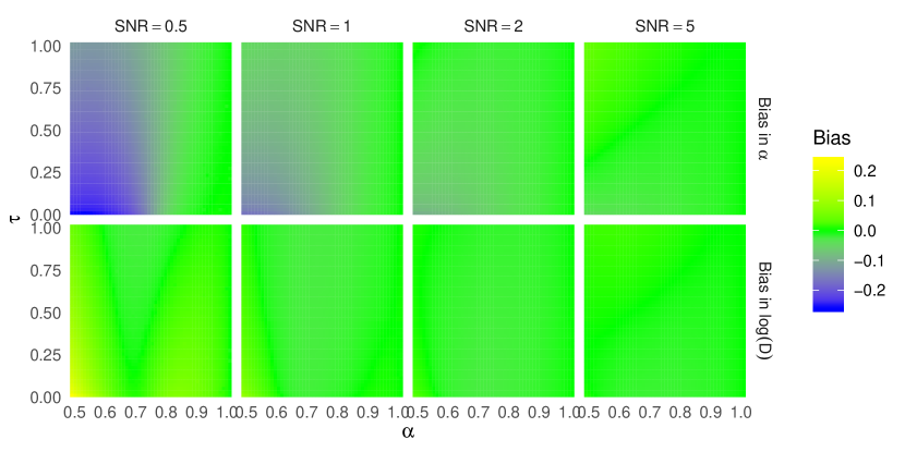
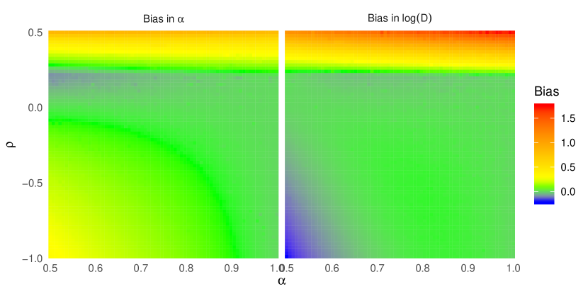
Figure 4: Model misspecification bias in $\alpha$ and $D$. (a) Best-fitting fMA model to true fSD models with different values of $\alpha$, $\tau$, and signal-to-noise ratio $\textnormal{SNR}=\operatorname{var}(\Delta B_{n}^{\alpha})/\sigma^{2}$. (b) Best-fitting fSD model to true fMA models with different values of $\alpha$ and $\rho$.

4 Simulation Study

In this section, we evaluate the performance of the proposed $\operatorname{ARMA}(p,q)$ high-frequency noise filters in various simulation settings. In each setting, we simulate $B=500$ observed data trajectories $\bm{Y}^{(b)}=(\bm{Y}^{(b)}_{0},\ldots,\bm{Y}^{(b)}_{N})$, $b=1,\ldots,B$, each consisting of $N=1800$ two-dimensional observations ($k=2$) recorded at intervals of $\Delta t=$1\text{/}60\text{\,}\mathrm{s}$$.

4.1 Empirical Localization Error

Consider the following simulation setting designed to reflect the localization errors in our own experimental setup. Let $\bm{Y}_{\textnormal{v}}$ denote the trajectory measurements for a particle undergoing ordinary diffusion in a viscous environment. Then we may estimate the MSD ratio

$$g(n)=\frac{\operatorname{\textsc{msd}}_{\tilde{\bm{Y}}_{\textnormal{v}}}(n)}{\operatorname{\textsc{msd}}_{\bm{X}_{\textnormal{v}}}(n)},$$ (4.1)

where the MSD of the true position process is $\operatorname{\textsc{msd}}_{\bm{X}_{\textnormal{v}}}(n)=2Dt$ with $D$ determined by the Stokes-Einstein relation (1.3), and the MSD of the drift-subtracted observation process $\tilde{\bm{Y}}_{\textnormal{v}}$ can be accurately estimated by

$$\widehat{\operatorname{\textsc{msd}}}_{\tilde{\bm{Y}}_{\textnormal{v}}}(n)=\frac{1}{M}\sum_{i=1}^{M}\widehat{\operatorname{\textsc{msd}}}_{\tilde{\bm{Y}}_{\textnormal{v}}^{(i)}}(n),$$

where $\widehat{\operatorname{\textsc{msd}}}_{\tilde{\bm{Y}}_{\textnormal{v}}^{(i)}}(n)$ is the empirical MSD (2.2) for each (drift-subtracted) particle trajectory $\tilde{\bm{Y}}_{\textnormal{v}}^{(1)},\ldots,\tilde{\bm{Y}}_{\textnormal{v}}^{(M)}$ recorded in a given experiment (e.g., Figure 1). We then suppose that the true trajectory is drift-free fBM $\bm{X}(t)=\bm{\Sigma}^{1/2}\bm{B}^{\alpha}(t)$, and simulate the measured trajectories from

$$\bm{Y}^{(b)}\stackrel{{\scriptstyle\textrm{iid}}}{{\sim}}\textnormal{MatNorm}\left(\bm{0},\bm{V},\bm{\Sigma}\right),$$

where $\bm{\Sigma}=\left[\begin{smallmatrix}1&0\\ 0&1\end{smallmatrix}\right]$ and the $(N+1)\times(N+1)$ variance matrix $\bm{V}$ is that of a CSI process with MSD given by

$$\operatorname{\textsc{msd}}_{\bm{Y}}(n)=(\gamma\hat{g}(n)-\gamma+1)\times\operatorname{\textsc{msd}}_{\bm{X}}(n),$$ (4.2)

where $\hat{g}(n)$ is the estimated noise ratio (4.1) from a viscous experiment, and the noise factor $\gamma>0$ can be used to suppress or amplify the empirical localization error with $\gamma<1$ or $\gamma>1$, respectively. Having constrained our estimator such that $\hat{g}(n)=1$ for $n>N_{0}$, (4.2) is a high-frequency noise model as defined by (3.1). Figure 5 displays the observed MSD (4.2) for a true fBM trajectory with $\alpha=0.6$, contaminated by empirical localization errors from two representative viscous experiments described in Table 3, illustrating the effects of high-frequency MSD suppression and amplification, respectively.

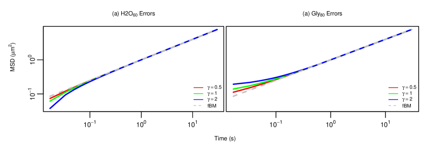
Figure 5: MSD of simulated observations with empirical localization error (4.2), where the true trajectory is an fBM process with $\alpha=0.6$. (a) High-frequency MSD suppression as observed in $\textnormal{H2O}_{60}$ experiment (see Table 3). (b) High-frequency MSD amplification as observed in $\textnormal{GLY}_{60}$ experiment.

The following methods are used to estimate the subdiffusion parameters $(\alpha,D)$ for each set of simulated particle observations $\bm{Y}^{(b)}$, $b=1,\ldots B$:

1. LS: The semiparameteric least-squares estimator (2.4) applied to the drift-subtracted empirical MSD (2.2).

2. fBM: The MLE of an fBM-driven location-scale model with linear drift,

   $$\bm{X}(t)=\bm{\mu}t+\bm{\Sigma}^{1/2}\bm{B}^{\alpha}(t),$$ (4.3)

   for which the model parameters are $(\alpha,\bm{\mu},\bm{\Sigma})$.

3. fSD: The MLE of the Savin-Doyle error model (2.17) applied to (4.3), for which the model parameters are $(\alpha,\tau,\sigma,\bm{\mu},\bm{\Sigma})$.

4. fMA: The MLE of the proposed $\operatorname{MA}(1)$ high-frequency noise filter (3.10) applied to (4.3), for which the model parameters are $(\alpha,\rho,\bm{\mu},\bm{\Sigma})$.

5. fMA2: The MLE of the proposed $\operatorname{MA}(2)$ high-frequency noise filter

   $$\bm{Y}_{n}=(1-\rho_{1}-\rho_{2})\bm{X}_{n}+\rho_{1}\bm{X}_{n-1}+\rho_{2}\bm{X}_{n-2}$$

   applied to (4.3), for which the model parameters are $(\alpha,\rho_{1},\rho_{2},\bm{\mu},\bm{\Sigma})$.

6. fARMA: The MLE of the proposed $\operatorname{ARMA}(1,1)$ high-frequency noise filter

   $$\bm{Y}_{n}=\theta\bm{Y}_{n-1}+(1-\theta-\rho)\bm{X}_{n}+\rho\bm{X}_{n-1}$$

   applied to (4.3), for which the model parameters are $(\alpha,\theta,\rho,\bm{\mu},\bm{\Sigma})$.

Remark 1.

The fSD exposure time parameter $\tau$ is typically known and therefore need not be estimated from the data. However, we have opted here to estimate it regardless, as this gives far greater ability to account for high-frequency MSD suppression (e.g., Figure 2). We return to this point in Section 5.

The point estimates for $(\alpha,D)$ for true fBM trajectories with $\alpha\in\{.6,.8,1\}$ and empirical error factor $\gamma\in\{.5,1,2\}$ are displayed in Figure 6.

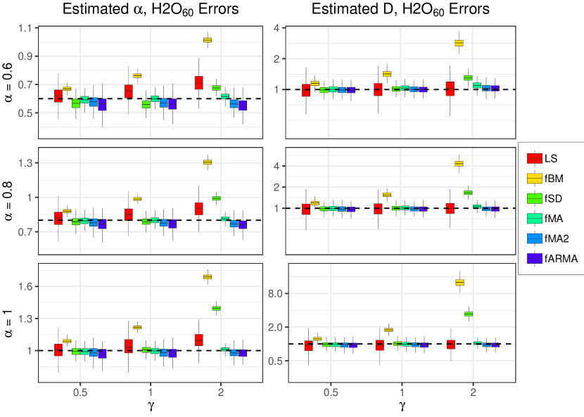
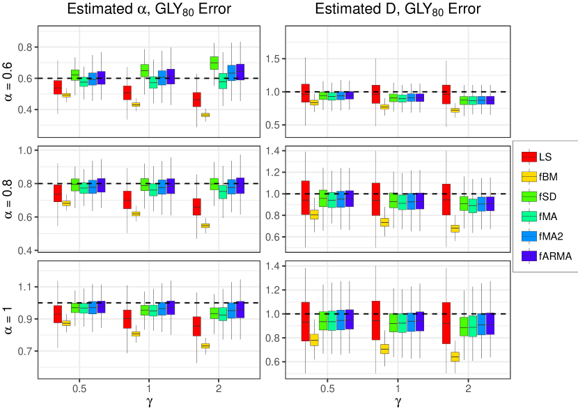
Figure 6: Estimates of $(\alpha,D)$ for true fBM trajectories with various types and degrees of empirical localization errors.

Table 1: Actual coverage by 95% confidence intervals with various types and degrees of empirical localization errors.

$\textnormal{P}_{95}(\alpha)$			$\textnormal{H2O}_{60}$ Errors				$\textnormal{GLY}_{80}$ Errors
			$\gamma=0.5$	$\gamma=1$	$\gamma=2$		$\gamma=0.5$	$\gamma=1$	$\gamma=2$
$\alpha=0.6$	fBM		5	0	0		0	0	0
	fSD		90	87	11		93	84	59
	fMA		96	96	90		91	88	88
	fMA2		91	91	84		94	95	94
	fARMA		92	93	87		89	93	93
$\alpha=0.8$	fBM		4	0	0		0	0	0
	fSD		91	93	0		92	94	94
	fMA		93	94	93		87	84	81
	fMA2		93	91	87		92	91	93
	fARMA		92	91	88		89	90	93
$\alpha=1$	fBM		1	0	0		0	0	0
	fSD		13	6	0		23	34	36
	fMA		95	94	93		87	81	70
	fMA2		92	92	94		90	88	84
	fARMA		91	92	92		87	86	85
$\textnormal{P}_{95}(\log D)$			$\textnormal{H2O}_{60}$ Errors				$\textnormal{GLY}_{80}$ Errors
			$\gamma=0.5$	$\gamma=1$	$\gamma=2$		$\gamma=0.5$	$\gamma=1$	$\gamma=2$
$\alpha=0.6$	fBM		57	1	0		20	1	0
	fSD		94	96	10		88	80	72
	fMA		96	95	88		86	73	85
	fMA2		94	95	95		86	79	66
	fARMA		94	95	95		87	79	65
$\alpha=0.8$	fBM		48	0	0		18	2	0
	fSD		92	94	1		90	89	82
	fMA		95	94	94		89	82	76
	fMA2		93	94	94		89	86	83
	fARMA		91	93	93		89	88	84
$\alpha=1$	fBM		42	0	0		16	1	0
	fSD		63	61	0		69	74	67
	fMA		95	94	95		90	88	80
	fMA2		92	92	94		91	90	85
	fARMA		90	91	93		91	89	85

As expected, the semiparametric LS estimator is substantially more variable than any of the fully parametric estimators, and the error-unadjusted fBM estimator incurs considerable bias, even with the smallest noise factor $\gamma=0.5$. The high-frequency estimators (fMA, fMA2, and fARMA) are fairly similar to each other, with the additional parameters of fMA2 and fARMA giving them slightly lower bias and higher variance. The high-frequency estimators are slightly more biased than fSD in the $\textnormal{GLY}_{80}$ simulation with $\alpha=0.8$. In contrast, they are somewhat less biased than fSD for $\textnormal{GLY}_{80}$ with the stronger subdiffusive signal $\alpha=0.6$, and considerably less so for $\textnormal{H2O}_{60}$ with the largest noise factor $\gamma=2$.

Table 1 displays the true coverage of the 95% confidence intervals for each parametric estimator, calculated as

$$\textnormal{P}_{95}(\psi)=\frac{1}{B}\sum_{b=1}^{B}\mathfrak{1}\{\theta\in\hat{\psi}_{b}\pm 1.96\operatorname{se}(\hat{\psi}_{b})\},$$

where $\psi\in\{\alpha,\log D\}$, $\hat{\psi}_{b}$ is the MLE for dataset $b$, and $\operatorname{se}(\hat{\psi}_{b})$ is the square root of the corresponding diagonal element of the variance estimator $\widehat{\operatorname{var}}(\hat{\bm{\theta}}_{b})=-\left[\frac{\partial^{2}\ell(\bm{Y}^{(b)}\mid\hat{\bm{\theta}}_{b})}{\partial\bm{\theta}\partial\bm{\theta}^{\prime}}\right]^{-1}$, where $\hat{\bm{\theta}}_{b}$ is the MLE of all model parameters. The true coverage of the fMA, fMA2, and fARMA confidence intervals is close to 95% when the bias is negligible and typically above 85%. This is also true for fSD, with the notable exception of either empirical error model and true $\alpha=1$. Upon closer inspection, we found that the fSD model suffers from an identifiability issue in the diffusive (viscous) regime, wherein the MSD suppression by $\tau$ and amplification by $\sigma$ achieve the same net effect over a range of values. This does not affect the estimate of $(\alpha,D)$, but significantly decreases the curvature of $\ell(\bm{Y}\mid\hat{\bm{\theta}})$, thus artifically inflating the observed Fisher information $\widehat{\operatorname{var}}(\hat{\bm{\theta}}_{b})^{-1}$.

Remark 2.

Since the subdiffusion equation $\operatorname{\textsc{msd}}_{\bm{X}}(t)=2Dt^{\alpha}$ dictates that $D$ be measured in units of $${\mathrm{\SIUnitSymbolMicro m}}^{2}\text{\,}\mathrm{s}$^{-\alpha}$, in order to compare estimates of $D$ for different values of $\alpha$ as in Figure 6, we follow the convention of interpreting $D$ as half the MSD at time $t=$1\text{\,}\mathrm{s}$$ (e.g., Lai et al., 2007; Wang et al., 2008), which for any $\alpha$ is measured uniformly in units of ${\mathrm{\SIUnitSymbolMicro m}}^{2}$.

4.2 Modeling Transient Subdiffusion

In this section, we show how the proposed high-frequency filter can be used not only for measurement error correction, but also to estimate subdiffusion in models where the power-law relation $\operatorname{\textsc{msd}}_{\bm{X}}(t)\sim t^{\alpha}$ holds only for $t>t_{\textnormal{min}}$. For this purpose, here we shall generate particle trajectories from a so-called Generalized Langevin Equation (GLE), a physical model derived from the fundamental laws of thermodynamics for interacting-particle systems (e.g., Kubo, 1966; Zwanzig, 2001; Kou, 2008). For a one-dimensional particle with negligible mass, the GLE for its trajectory $X(t)$ is a stochastic integro-differential equation of the form

$$\int_{-\infty}^{t}\phi(t-s)V(s)\mathop{}\!\mathrm{d}s=F(t),$$ (4.4)

where $V(t)=\frac{\mathop{}\!\mathrm{d}}{\mathop{}\!\mathrm{d}t}X(t)$ is the particle velocity, $\phi(t)$ is a memory kernel, and $F(t)$ is a stationary mean-zero Gaussian force process with $\operatorname{\textsc{acf}}_{F}(t)=k_{B}T\cdot\phi(t)$, where $T$ is temperature and $k_{B}$ is Boltzmann’s constant. The memory of the process is modeled as a generalized Rouse kernel (McKinley et al., 2009):

$$\phi(t)=\frac{\nu}{K}\sum_{k=1}^{K}\exp(-|t|/\tau_{k}),\quad\tau_{k}=\tau\cdot(K/k)^{\gamma}.$$ (4.5)

The sum-of-exponentials form of (4.5) is a longstanding linear model for viscoelastic relaxation (e.g., Soussou et al., 1970; Ferry, 1980; Mason and Weitz, 1995), whereas the specific parametrization of the relaxation modes $\tau_{k}$ has been shown for sufficiently large $K$ to exhibit transient subdiffusion (McKinley et al., 2009),

$$\operatorname{\textsc{msd}}_{X}(t)=\begin{cases}2D_{\textnormal{eff}}\cdot t^{\alpha_{\textnormal{eff}}}&t_{\textnormal{min}}<t<t_{\textnormal{max}}\\ 2D_{\textnormal{min}}\cdot t&t<t_{\textnormal{min}}\\ 2D_{\textnormal{max}}\cdot t&t>t_{\textnormal{max}},\end{cases}$$ (4.6)

where the subdiffusive range parameters $(t_{\textnormal{min}},t_{\textnormal{max}})$ and the effective subdiffusion parameters $(\alpha_{\textnormal{eff}},D_{\textnormal{eff}})$ are implicit functions of $K$, $\gamma$, $\tau$, and $\nu$. Details of the parameter conversions and the exact form of (4.6) are provided in Appendix D.

Figure 7 displays the MSD of various GLE processes with fixed $K=300$, and $\{\gamma,\tau,\nu\}$ tuned to have $\alpha_{\textnormal{eff}}=0.63$, $D_{\textnormal{eff}}=0.58$, and values of $t_{\textnormal{min}}/\Delta t=\{5,10,20,50,100\}$. In all cases the value of $t_{\textnormal{max}}$ was several times larger than the experimental timeframe $N\Delta t=$30\text{\,}\mathrm{s}$$, such that the observable MSD could potentially be matched by the fBM-driven high-frequency models of Section 3. The trajectories for this experiment were simulated from

$$\bm{Y}^{(b)}\stackrel{{\scriptstyle\textrm{iid}}}{{\sim}}\textnormal{MatNorm}(\bm{0},\bm{V},\bm{\Sigma}),$$

where $\bm{\Sigma}=\left[\begin{smallmatrix}1&0\\ 0&1\end{smallmatrix}\right]$ and $\bm{V}$ is the $(N+1)\times(N+1)$ variance matrix of the GLE process (4.4) with MSDs displayed in Figure 7.

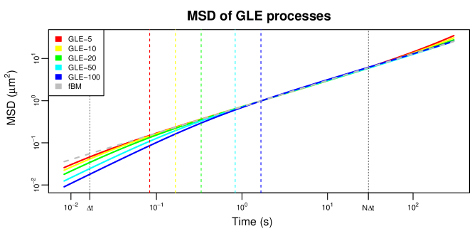
Figure 7: MSD of GLE processes with $\alpha_{\textnormal{eff}}=0.63$, $D_{\textnormal{eff}}=0.58$, and $t_{\textnormal{min}}/\Delta t=\{5,10,20,50,100\}$. The horizontal dashed lines indicated $t_{\textnormal{min}}$, and the diagonal dashed line corresponds to an fBM process with the same subdiffusive parameters $(\alpha_{\textnormal{eff}},D_{\textnormal{eff}})$. The dotted vertical lines indicate the beginning and end of experiment, at $\Delta t=$1\text{/}60\text{\,}\mathrm{s}$$ and $N\Delta t=$30\text{\,}\mathrm{s}$$, respectively.

Figure 8 displays the parameter estimates of $\alpha_{\textnormal{eff}}$ and $D_{\textnormal{eff}}$ for the six estimators described in Section 4.1, and Table 2 displays the true coverage probabilities of the corresponding 95% confidence intervals.

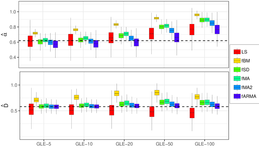
Figure 8: Estimates of $\alpha_{\textnormal{eff}}$ and $D_{\textnormal{eff}}$ for simulated GLE trajectories with true parameters $\alpha_{\textnormal{eff}}=0.63$, $D_{\textnormal{eff}}=0.58$, $K=300$, and $t_{\textnormal{min}}/\Delta t=\{5,10,20,50,100\}$.

Table 2: Actual coverage by 95% confidence intervals with different GLE processes.

$\textnormal{P}_{95}(\alpha)$	GLE-5	GLE-10	GLE-20	GLE-50	GLE-100
fBM	0	0	0	0	0
fSD	96	96	64	0	0
fMA	95	84	25	0	0
fMA2	92	95	89	15	0
fARMA	92	92	95	85	53
$\textnormal{P}_{95}(\log D)$	GLE-5	GLE-10	GLE-20	GLE-50	GLE-100
fBM	31	8	1	1	11
fSD	94	95	87	78	74
fMA	93	92	78	68	81
fMA2	94	95	93	93	92
fARMA	93	94	93	95	91

As in Figure 6, the LS estimator has the highest variance and fBM the largest bias. In this case, however, the fSD and fMA estimators exhibit considerable bias in estimating $\alpha$, especially when $t_{\textnormal{min}}\gg\Delta t$. In contrast, the fARMA estimator displays good accuracy and reasonable coverage even when $t_{\textnormal{min}}$ is $50\times$ the interobservation time $\Delta t$.

5 Analysis of Experimental Data

We now investigate the performance of our high-frequency filters on a variety of real single-particle tracking experiments described in Table 3. For each experiment, Table 3 reports the interobservation time $\Delta t$, the number of particles $M$, the number of observations per trajectory $N$, and the type of camera and particle tracking software. All tracked particles are inert polystyrene beads of diameter $d=$1\text{\,}\mathrm{\SIUnitSymbolMicro m}$$.

Table 3: Summary of experimental conditions for various single-particle tracking experiments. The different types of fluids are water (H2O), glycerol (GLY), mucus from human bronchial ephithelia cell cultures (HBE), and polyethilene oxide (PEO). The subscripts correspond to sampling frequency for H2O, percent concentration for GLY, and percent weight (wt%) for HBE and PEO. The two types of cameras are Flea3 USB 3.0 (Flea3: FLIR, 2019) and Panoptes (Pan: CISMM, 2019a). The particle tracking software employed is either Video Spot Tracker (VS: CISMM, 2019b) or Net Tracker (Net: Newby et al., 2018).

Medium	Name	$D$	$\Delta t$ (s)	$N$	$M$	Camera	Software
Viscous	$\textnormal{H2O}_{15}$	0.43	1/15	1800	1293	Flea3	Net
($\alpha=1$)	$\textnormal{H2O}_{30}$	0.43	1/30	1800	889	Flea3	Net
	$\textnormal{H2O}_{60}$	0.43	1/60	1800	1931	Flea3	Net
	$\textnormal{H2O}_{60b}$	0.43	1/60	1800	313	Flea3	VS
	$\textnormal{GLY}_{60}$	0.09	1/60	1800	532	Flea3	VS
	$\textnormal{GLY}_{80}$	0.022	1/60	1800	358	Flea3	VS
Viscoelastic	$\textnormal{HBE}_{1.5}$	-	1/60	1800	63	Flea3	VS
($\alpha$ unknown)	$\textnormal{HBE}_{2}$	-	1/60	1800	72	Flea3	VS
	$\textnormal{HBE}_{2.5}$	-	1/60	1800	76	Flea3	VS
	$\textnormal{HBE}_{3}$	-	1/60	1800	99	Flea3	VS
	$\textnormal{HBE}_{4}$	-	1/60	1800	180	Flea3	VS
	$\textnormal{HBE}_{5}$	-	1/60	1800	178	Flea3	VS
	$\textnormal{PEO}_{0.22}$	-	1/38.17	1145	123	Pan	VS
	$\textnormal{PEO}_{0.45}$	-	1/38.17	1145	205	Pan	VS
	$\textnormal{PEO}_{0.6}$	-	1/38.17	1145	192	Pan	VS
	$\textnormal{PEO}_{0.75}$	-	1/38.17	1145	202	Pan	VS
	$\textnormal{PEO}_{0.9}$	-	1/38.17	1145	124	Pan	VS
	$\textnormal{PEO}_{1.22}$	-	1/38.17	1145	193	Pan	VS

5.1 Viscous Fluids

The first six experiments are conducted in viscous fluids (water and glycerol), for which $\alpha=1$ and the diffusivity constant $D$ is derived from the Stokes-Einstein relation (1.3). For the six estimators described in Section 4.1, estimates of $(\alpha,D)$ and true coverage probabilities of the associated 95% confidence intervals are displayed in Figure 9 and Table 4, respectively.

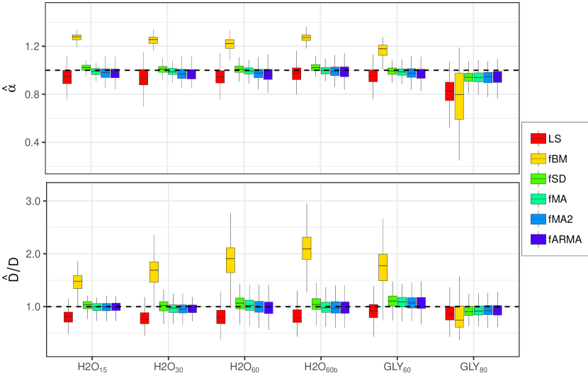
Figure 9: Estimates of $(\alpha,D)$ for the viscous medium experiments in Table 3.

Table 4: Actual coverage by $95\%$ confidence intervals in viscous fluid study.

	$\textnormal{H2O}_{15}$	$\textnormal{H2O}_{30}$	$\textnormal{H2O}_{60}$	$\textnormal{H2O}_{60b}$	$\textnormal{GLY}_{60}$	$\textnormal{GLY}_{80}$
fBM	0	0	0	0	4	16
fSD	47	42	47	11	14	44
fMA	94	90	93	85	90	71
fMA2	95	91	92	87	91	75
fARMA	95	92	94	88	92	82

Table 5: Ratio of true and estimated exposure time to interobservation time for the fSD model in the viscous medium experiments of Table 3.

	$\textnormal{H2O}_{15}$	$\textnormal{H2O}_{30}$	$\textnormal{H2O}_{60}$	$\textnormal{H2O}_{60b}$	$\textnormal{GLY}_{60}$	$\textnormal{GLY}_{80}$
True $\tau/\Delta t$	$0.3$	$0.3$	$0.3$	$0.3$	$0.3$	$0.3$
Estimated $\hat{\tau}/\Delta t$	0.93	0.91	0.89	0.91	0.85	0.54

Both fSD and the proposed high-frequency estimators remove most of the bias of fBM without camera error correction. However, the fSD 95% confidence intervals suffer from severe undercoverage, due to the parameter identifiability issue noted in Section 4.1. Indeed, Table 5 shows that the estimated exposure time $\hat{\tau}$ is much larger than its true value $\tau$, as required in the H2O experiments to capture high-frequency MSD suppression. When $\tau$ is fixed at its true value, fSD estimation results are close those of fBM, as illustrated in Figure 1.

5.2 Viscoelastic Fluids

The remaining 12 experiments from Table 3 are conducted in two kinds of viscoelastic media. The first consists of mucus harvested from primary human bronchial epithelial (HBE) cell cultures (Hill et al., 2014b). Washings from cultures were pooled and concentrated to desired weight percent solids (wt%). Higher concentrations of solids in lung mucus have been associated with disease states, so an accurate recovery of biophysical properties is critical in samples with volumes too small to measure wt% directly (Hill et al., 2014b). The second medium, polyethylene oxide (PEO), is a synthetic polyether compound with applications in diverse fields ranging from biomedicine to industrial manufacturing (Working et al., 1997). The present data consists of trajectories in 5 megadalton ($\mathrm{MDa}$) PEO at a range of wt% values. In all 12 viscoelastic experiments, subdiffusive motion $\alpha<1$ is expected, but the true values of $(\alpha,D)$ are unknown.

Figure 10 displays the various estimates of $(\alpha,D)$ for the viscoelastic data. The high-frequency noise models tend to produce similar results, with the largest differences occurring in the estimates of $\alpha$ at high wt%. In the absence of true values of $(\alpha,D)$ against which to benchmark our models, we compare the different subdiffusion estimators using the following metric.

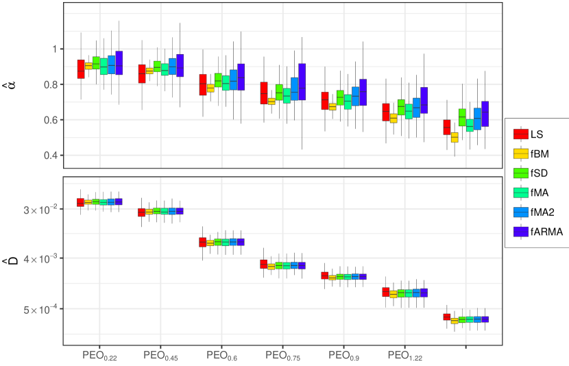
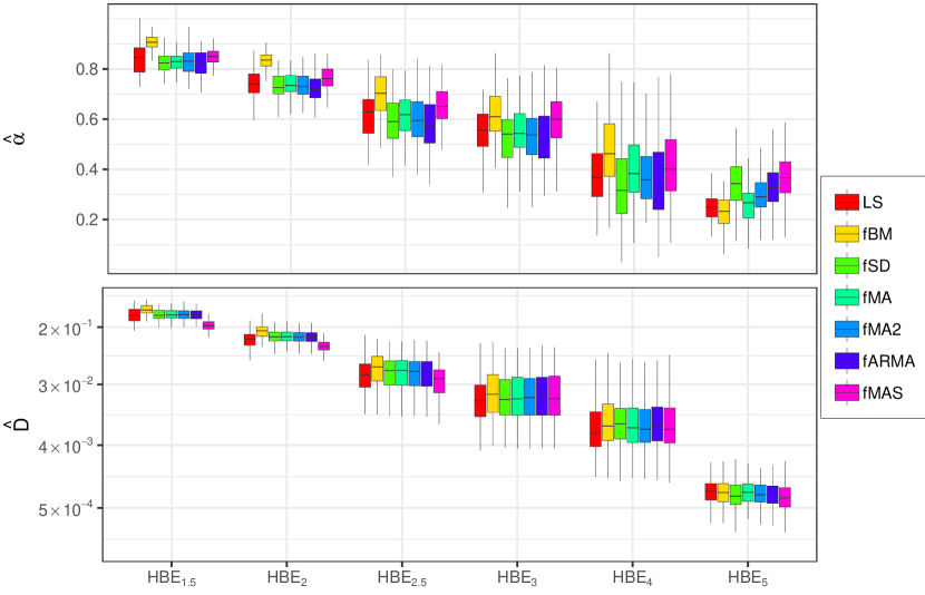
Figure 10: Estimates of $(\alpha,D)$ for the viscoelastic medium experiments in Table 3. For the HBE data, the subdiffusive estimators are the six described in Section 4.1, and that of the fMA + static noise (fMAS) model (5.2).

For measurements $\bm{Y}=(\bm{Y}_{0},\bm{Y}_{1},\ldots,\bm{Y}_{N})$ of a given particle trajectory, let $\bm{Y}_{(r)k}=(\bm{Y}_{k},\bm{Y}_{k+r},\ldots,\bm{Y}_{k+\lfloor N/r\rfloor r})$ denote the $k$th subset of the measurements downsampled by a factor of $r$. Downsampling effectively removes all high-frequency dynamics from the particle positions, leading us initially to consider a subdiffusion estimator which maximizes the composite loglikelihood (e.g., Varin et al., 2011)

$$\ell_{\textnormal{C}}^{(r)}(\bm{\theta}\mid\bm{Y})=\sum_{k=0}^{r-1}\ell_{\textnormal{fBM}}(\bm{\theta}\mid\bm{Y}_{(r)k}),$$

where $\bm{\theta}=(\alpha,\bm{\beta},\bm{\Sigma})$ are the parameters of the location-scale fBM model (2.6). However, this estimator was found to have very high variance, which, for the purpose of constructing confidence intervals, was poorly estimated by the sandwich method (Freedman, 2006). Therefore, we have not pursued this downsampling estimator here. Instead, we propose to evaluate the accuracy of subdiffusive model $M_{j}$ by calculating

$$\ell_{\textnormal{C}}^{(r)}(\hat{\bm{\theta}}^{(M_{j})}\mid\bm{Y}),$$ (5.1)

where $\hat{\bm{\theta}}^{(M_{j})}$ are the corresponding elements of the MLE under $M_{j}$ for the complete set of measurements $\bm{Y}$. Larger values of the composite likelihood statistic (5.1) indicate better agreement with subdiffusive dynamics $\operatorname{\textsc{msd}}_{\bm{X}}(t)=2D\cdot t^{\alpha}$ for $t>\Delta t\times r$. This approach to comparing models with respect to $(\alpha,D)$ is evocative of the focused information criterion of Claeskens and Hjort (2003).

Table 6 reports the improvement in the composite likelihood statistic (5.1) of each measurement error model $M_{j}$ over the noise-free fBM model,

$$\mathcal{S}^{(r)}=\frac{1}{M}\sum_{m=1}^{M}\Big{\{}\ell_{\textnormal{C}}^{(r)}(\hat{\bm{\theta}}^{(M_{j})}\mid\bm{Y}^{(m)})-\ell_{\textnormal{C}}^{(r)}(\hat{\bm{\theta}}^{(\textnormal{fBM})}\mid\bm{Y}^{(m)})\Big{\}},$$

where the average is calculated over the trajectories $\bm{Y}^{(1)},\ldots,\bm{Y}^{(M)}$ in each viscoelastic experiment of Table 3. Interpretation of the units in Table 6 is similar to those of the AIC, upon multiplying ours by a factor of negative two. However, we do not penalize by the number of parameters here, since all models have the same number of parameters in the subdiffusive range of interest. We return to this point in the Discussion (Section 6).

Table 6: Average improvement $\mathcal{S}^{(r)}$ in the composite likelihood statistic (5.1) relative to fBM for various subdiffusion estimators. For each experiment and downsampling factor $r$, the estimator with the greatest improvement is highlighted in bold.

PEO			$0.22$	$0.45$	$0.6$	$0.75$	$0.9$	$1.22$
$r=5$	fSD		3.1	2.9	4.2	4.3	3.6	7.6
	fMA		2.9	2.5	3.7	4.3	3.8	11
	fMA2		4.1	4.6	5.8	5.1	4.8	9.9
	fARMA		4.8	3.9	6.9	5.2	3.8	12
$r=10$	fSD		2.2	2	2.9	3.5	2.9	5.7
	fMA		1.8	1.9	2.5	3.1	2.5	8.7
	fMA2		2.7	3.4	4.5	3.6	3.6	7.9
	fARMA		2.7	3	4.7	3.5	2.8	7.7
$r=20$	fSD		1.6	1.6	2.9	2.4	2.6	4.2
	fMA		1.7	1.6	2.3	2.4	1.9	7
	fMA2		1.5	2.7	3.9	3.3	2.8	6.1
	fARMA		1.5	1.7	3.3	2	1.7	5
HBE			$1.5$	$2$	$2.5$	$3$	$4$	$5$
$r=5$	fSD		15	29	31	28	29	-60
	fMA		15	27	30	28	42	0.06
	fMA2		15	31	31	29	47	-9.6
	fARMA		16	31	30	29	33	-22
	fMAS		15	30	31	29	32	-72
$r=10$	fSD		11	21	23	18	12	-53
	fMA		11	20	22	21	30	0.25
	fMA2		12	22	21	22	31	-7.1
	fARMA		11	22	22	20	18	-26
	fMAS		11	21	23	19	13	-42
$r=20$	fSD		9	14	16	11	2.5	-61
	fMA		8.9	14	16	18	23	0.81
	fMA2		8.9	17	15	16	22	-5.3
	fARMA		8.1	16	14	11	7.1	-28
	fMAS		9	14	15	16	11	-52
$r=60$	fSD		2.3	4.1	5.7	4.1	2.3	8
	fMA		2.1	4.3	6.2	6.0	8.5	1.3
	fMA2		2.3	5.7	5.1	5.3	9.2	5.3
	fARMA		2.9	5.1	5.4	4.1	2.7	4
	fMAS		2.5	4.5	5.6	5.0	3.3	12

As expected, noise correction produces significantly better estimates of $(\alpha,D)$ than does the fBM model alone. For the PEO data, the more accurate subdiffusion estimators are fMA2 and fARMA, whereas for HBE they are fMA and fMA2. A notable exception is in the highest concentration HBE at 5 wt%, where for $r=5,10,20$ all measurement error models except fMA are decisively dominated by noise-free fBM. To see why this is the case, Figure 11 displays the empirical MSDs of three representative particle trajectories from the HBE 5 wt% dataset. Each of these MSDs exhibits two distinct power-law signatures, with the changepoint occurring around $t=$1\text{\,}\mathrm{s}$$. Figure 11 displays the fitted MSD for various subdiffusion estimators. We can see that fBM and fMA capture only the short-range power-law dynamics, whereas the other estimators capture the power law for $t>$1\text{\,}\mathrm{s}$$. However, for $r=5,10,20$, a sufficient amount of short-range power-law remains for it to outweigh the contribution of the longer-range dynamics in the calculation of the composite likelihood statistic (5.1), thus favoring the fMB and fMA models.

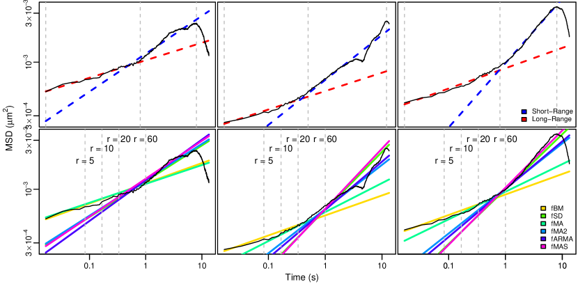
Figure 11: (a) Pathwise empirical MSD for 3 representative particles of diameter $1\text{\,}\mathrm{\SIUnitSymbolMicro m}$ with 5 wt% mucus concentration, and their transient subdiffusion of two phases. The change point between two phases varies across particles. (b) Empirical MSD and fitted subdiffusion with different methods, where the subdiffusion is computed using the power-law: $\operatorname{\textsc{msd}}(t)=2D\times t^{\alpha}$ and $(\alpha,D)$ is extracted from parametric estimations. Vertical dotted lines for different downsampling rates $r$ are also demonstrated.

It is theorized that the presence of two distinct power-law signatures in the HBE 5 wt% data is due to the extremely low particle mobility, such that the trajectory displacement signal is substantially masked by the measurement noise floor. To investigate this, we added the static noise component of the Savin-Doyle model to the fMA model, leading to the so-called fMAS model

$$\bm{Y}_{n}=(1-\rho)\bm{X}_{n}+\rho\bm{X}_{n-1}+\bm{\varepsilon}_{n}.$$ (5.2)

Indeed, Table 6 indicates that fMAS most accurately captures long-range subdiffusion dynamics for $r=60$. It is noteworthy that fMAS outperforms the Savin-Doyle model (fSD) in this setting, suggesting that noise sources other than static and dynamic errors may be present in these data.

6 Discussion

We present a family of parametric filters to correct for high-frequency noise in single-particle tracking measurements. We demonstrate theoretically that our models can account for a very broad range of localization errors, and show how to combine them with arbitrary models of particle dynamics and low-frequency drift, so as to estimate subdiffusion parameters in a computationally efficient manner.

Compared to the state-of-the-art Savin-Doyle error model, our high-frequency filters generally exhibit lower bias, and much better coverage of confidence intervals for $\alpha\approx 1$, where the Savin-Doyle model suffers from a parameter identifiability issue. A notable setting in which the Savin-Doyle model outperforms ours is when static noise dominates the high-frequency errors, e.g., in low-mobility experiments such as HBE 5 wt%. Indeed, static noise is only covered by our definition of high-frequency noise (3.1) if the true position process $\bm{X}(t)$ is nonstationary (as is the case for fBM). However, it is easy to combine static noise with our parametric filters without sacrificing computational efficiency, as we have done for the fMAS model in Section 5.2.

An important practical question is how to determine which high-frequency error model produces the most accurate subdiffusion estimator for a given viscoelastic fluid and instrumental setup. We have proposed a composite likelihood metric to approach this problem, but accounting for model complexity in the underlying estimation of Kullback-Liebler divergence would benefit from deeper theoretical and empirical investigation. Possible directions of inquiry for the former are AIC for composite likelihoods (Varin et al., 2011) and with consistent estimators (Grønneberg and Hjort, 2014), as well as focused information criteria for time series models (Hermansen et al., 2015).

Appendix A Profile Likelihood for the Matrix-Normal Distribution

Let $\Delta\bm{X}_{N\times k}=(\Delta\bm{X}_{0},\ldots,\Delta\bm{X}_{N-1})$ denote the increments of the location-scale model (2.6) in matrix form. Then $\Delta\bm{X}$ follows a matrix-normal distribution (2.11)

$$\Delta\bm{X}\sim\textnormal{MatNorm}(\bm{F}\bm{\beta},\bm{V}_{\bm{\varphi}},\bm{\Sigma})$$ (A.1)

$$\iff\qquad\operatorname{vec}(\Delta\bm{X}) \sim\mathcal{N}(\operatorname{vec}(\bm{F}\bm{\beta}),\bm{\Sigma}\otimes\bm{V}_{\bm{\varphi}}),$$

where $\operatorname{vec}(\Delta\bm{X})$ concatenates the columns of $\Delta\bm{X}$ into a vector of length $Nk$, similarly for $\operatorname{vec}(\bm{F}\bm{\beta})$, and $\otimes$ denotes the Kronecker matrix product.

As shown in Lysy et al. (2016), the parameters $\bm{\theta}=({\bm{\varphi}},\bm{\beta},\bm{\Sigma})$ of (A.1) can be efficiently estimated using a profile likelihood. Consider a generalized matrix-normal model

$$\bm{Y}_{N\times k}\sim\textnormal{MatNorm}(\bm{F}_{\bm{\varphi}}\bm{\beta},\bm{V}_{\bm{\varphi}},\bm{\Sigma}),$$

where both the design matrix $\bm{F}_{\bm{\varphi}}$ and the row-wise covariance $\bm{V}_{\bm{\varphi}}$ depend on ${\bm{\varphi}}$. Then for fix ${\bm{\varphi}}$, the conditional MLE of $(\bm{\beta},\bm{\Sigma})$ is given by

$$\hat{\bm{\beta}}_{{\bm{\varphi}}}=(\bm{F}_{\bm{\varphi}}^{\prime}\bm{V}_{\bm{\varphi}}^{-1}\bm{F}_{\bm{\varphi}})^{-1}\bm{F}_{\bm{\varphi}}^{\prime}\bm{V}_{\bm{\varphi}}^{-1}\bm{Y}$$ (A.2)

$$\hat{\bm{\Sigma}}_{{\bm{\varphi}}}=\frac{1}{N}(\bm{Y}-\bm{F}_{\bm{\varphi}}\hat{\bm{\beta}}_{{\bm{\varphi}}})^{\prime}\bm{V}_{\bm{\varphi}}^{-1}(\bm{Y}-\bm{F}_{\bm{\varphi}}\hat{\bm{\beta}}_{{\bm{\varphi}}}),$$

from which we may calculate the profile loglikelihood

$$\ell_{\textnormal{prof}}({\bm{\varphi}}\mid\bm{Y}) =\ell({\bm{\varphi}},\bm{\beta}=\hat{\bm{\beta}}_{{\bm{\varphi}}},\bm{\Sigma}=\hat{\bm{\Sigma}}_{{\bm{\varphi}}}\mid\bm{Y})$$ (A.3)

$$=-\tfrac{1}{2}\big{\{}k\log|\bm{V}_{\bm{\varphi}}|+N\log|\hat{\bm{\Sigma}}_{{\bm{\varphi}}}|+Nk\big{\}}.$$

Upon solving the reduced optimization problem $\hat{\bm{\varphi}}=\operatorname*{arg\,max}_{{\bm{\varphi}}}\ell_{\textnormal{prof}}({\bm{\varphi}}\mid\bm{Y})$, we obtain $\hat{\bm{\theta}}=(\hat{\bm{\varphi}},\bm{\beta}_{\hat{\bm{\varphi}}},\bm{\Sigma}_{\hat{\bm{\varphi}}})$ as the MLE of the full likelihood $\ell(\bm{\theta}\mid\bm{Y})$. This technique can be used for all the measurement error models presented in this paper.

Appendix B Inference for the fSD Model

The $k$-dimensional fSD model (2.17) takes the form

$$\bm{X}(t) =\sum_{j=1}^{d}\bm{\beta}_{j}f_{j}(t)+\bm{\Sigma}^{1/2}\bm{Z}(t),$$ (B.1)

$$\bm{Y}_{n} =\frac{1}{\tau}\int_{0}^{\tau}\bm{X}(t_{n}-s)\mathop{}\!\mathrm{d}s+\bm{\varepsilon}_{n},$$

where $t_{n}=n\cdot\Delta t$, $\bm{Z}(t)=\big{(}Z_{1}(t),\ldots,Z_{k}(t)\big{)}$ with $Z_{i}(t)\stackrel{{\scriptstyle\textrm{iid}}}{{\sim}}B_{\alpha}(t)$, and $\bm{\varepsilon}_{n}\stackrel{{\scriptstyle\textrm{iid}}}{{\sim}}\mathcal{N}(\bm{0},\sigma^{2}\cdot\bm{\Sigma})$ are independent of $\bm{Z}(t)$. Letting $\Delta\bm{Y}_{n}=\bm{Y}_{n+1}-\bm{Y}_{n}$, we can rewrite (B.1) to obtain

$$\Delta\bm{Y}_{n}=\sum_{j=1}^{d}\bm{\beta}_{j}\Delta f^{\star}_{nj}+\bm{\Sigma}^{1/2}(\Delta\bm{Z}^{\star}_{n}-\Delta\bm{\eta}_{n}),$$

where

$$f^{\star}_{nj}=\frac{1}{\tau}\int_{0}^{\tau}f_{j}(t_{n}-s)\mathop{}\!\mathrm{d}s,\qquad Z_{ni}^{\star}=\frac{1}{\tau}\int_{0}^{\tau}Z_{i}(t_{n}-s)\mathop{}\!\mathrm{d}s,$$

and $\bm{\eta}_{n}=\bm{\Sigma}^{-1/2}\bm{\varepsilon}_{n}\stackrel{{\scriptstyle\textrm{iid}}}{{\sim}}\mathcal{N}(\bm{0},\sigma^{2}\bm{I}_{d})$. Thus we have $f^{\star}_{nj}=\frac{1}{\tau}\int_{0}^{\tau}f_{j}(t_{n}-s)\mathop{}\!\mathrm{d}s$, $\bm{Z}^{\star}_{n}=(Z_{n1}^{\star},\ldots Z_{nk}^{\star})$ with $Z_{ni}^{\star}=\frac{1}{\tau}\int_{0}^{\tau}Z_{i}(t_{n}-s)\mathop{}\!\mathrm{d}s$, and $\bm{\eta}_{n}=\bm{\Sigma}^{-1/2}\bm{\varepsilon}_{n}\stackrel{{\scriptstyle\textrm{iid}}}{{\sim}}\mathcal{N}(\bm{0},\sigma^{2}\bm{I}_{d})$. Thus, we have

$$\Delta\bm{Y}_{N\times k}\sim\textnormal{MatNorm}(\bm{F}\bm{\beta},\bm{V}_{{\bm{\varphi}}},\bm{\Sigma}),$$ (B.2)

where $\bm{F}_{N\times d}$ has elements $\bm{F}_{nj}=\Delta f^{\star}_{nj}$, $\bm{V}_{{\bm{\varphi}}}$ is a variance matrix parametrized by ${\bm{\varphi}}=(\alpha,\tau,\sigma)$ with elements

$$\bm{V}_{{\bm{\varphi}}}^{(n,m)} =\operatorname{cov}(\Delta Z^{\star}_{ni}+\Delta\eta_{ni},\Delta Z^{\star}_{mi}+\Delta\eta_{mi})$$

$$=\operatorname{cov}(\Delta Z^{\star}_{ni},\Delta Z^{\star}_{mi})+\operatorname{cov}(\Delta\eta_{ni},\Delta\eta_{mi}).$$

To finish the calculations, without loss of generality we may focus on the one-dimensional case $Z_{i}(t)=Z(t)=B_{\alpha}(t)$ and $\eta_{in}=\eta_{n}\stackrel{{\scriptstyle\textrm{iid}}}{{\sim}}\mathcal{N}(0,\sigma^{2})$. Thus we have

$$\operatorname{cov}(Z_{n}^{\star},Z_{m}^{\star}) =E[Z_{n}^{\star}Z_{m}^{\star}]$$

$$=\frac{1}{\tau^{2}}E\left[\int_{0}^{\tau}Z(t_{n}-s)\mathop{}\!\mathrm{d}s\cdot\int_{0}^{\tau}Z(t_{m}-u)\mathop{}\!\mathrm{d}u\right]$$

$$=\frac{1}{\tau^{2}}E\left[\int_{0}^{\tau}\int_{0}^{\tau}Z(t_{n}-s)Z(t_{m}-u)\mathop{}\!\mathrm{d}s\mathop{}\!\mathrm{d}u\right]$$

$$=\frac{1}{\tau^{2}}\int_{0}^{\tau}\int_{0}^{\tau}E\left[Z(t_{n}-s)Z(t_{m}-u)\right]\mathop{}\!\mathrm{d}s\mathop{}\!\mathrm{d}u,$$

where the last line is obtained from the Fubini-Tonelli theorem, since by Cauchy-Schwarz we have

$$\int_{0}^{\tau}\int_{0}^{\tau}E\Big{[}|Z(t_{n}-s)Z(t_{m}-u)|\Big{]}\mathop{}\!\mathrm{d}s\mathop{}\!\mathrm{d}u \leq\sqrt{\int_{0}^{\tau}E[Z(t_{n}-s)^{2}]\mathop{}\!\mathrm{d}s\cdot\int_{0}^{\tau}E[Z(t_{m}-u)^{2}]\mathop{}\!\mathrm{d}u}$$

$$=\sqrt{\int_{0}^{\tau}\operatorname{\textsc{msd}}_{Z}(t_{n}-s)\mathop{}\!\mathrm{d}s\cdot\int_{0}^{\tau}\operatorname{\textsc{msd}}_{Z}(t_{m}-u)\mathop{}\!\mathrm{d}u},$$

and the right-hand side is finite as long as $\operatorname{\textsc{msd}}_{Z}(t)$ is continuous for $t\geq 0$. Thus, for the fBM process $Z(t)=B_{\alpha}(t)$ we have

$$\operatorname{cov}(Z^{\star}_{n},Z^{\star}_{m}) =\frac{1}{2\tau^{2}}\int_{0}^{\tau}\int_{0}^{\tau}(t_{n}-s)^{\alpha}+(t_{m}-u)^{\alpha}-|(t_{n}-t_{m})-(s-u)|^{\alpha}\mathop{}\!\mathrm{d}s\mathop{}\!\mathrm{d}u$$

$$=h_{\tau}(t_{n})+h_{\tau}(t_{m})-g_{\tau}(t_{n}-t_{m}),$$

where

$$g_{\tau}(t)=\frac{|t+\tau|^{\alpha+2}+|t-\tau|^{\alpha+2}-2|t|^{\alpha+2}}{2\tau^{2}(\alpha+1)(\alpha+2)},\qquad h_{\tau}(t)=\frac{(t-\tau)^{\alpha}-t^{\alpha}}{2\tau(\alpha+1)}.$$

Finally, since for any increment process $\Delta X_{n}$ we have

$$\operatorname{cov}(\Delta X_{n},\Delta X_{m})=E\left[X_{n+1}X_{m+1}\right]-E\left[X_{n+1}X_{m}\right]-E\left[X_{n}X_{m+1}\right]+E\left[X_{n}X_{m}\right],$$ (B.3)

we may calculate that

$$\operatorname{\textsc{acf}}_{\Delta Z^{\star}}(n)=\operatorname{cov}(\Delta Z^{\star}_{n},\Delta Z^{\star}_{m+n})=g_{\tau}(|n+1|\Delta t)+g_{\tau}(|n-1|\Delta t)-2g_{\tau}(|n|\Delta t).$$ (B.4)

Similarly, we obtain

$$\operatorname{\textsc{acf}}_{\Delta\eta}(n)=\sigma^{2}\times\big{\{}2\cdot\mathfrak{1}(n=0)-\mathfrak{1}(n=1)\big{\}},$$

such that $\bm{V}_{{\bm{\varphi}}}$ is a Toeplitz matrix with elements

$$\bm{V}_{{\bm{\varphi}}}^{(n,m)}=\operatorname{\textsc{acf}}_{\Delta Z^{\star}}(n-m)+\operatorname{\textsc{acf}}_{\Delta\eta}(n-m).$$

Appendix C Calculations for ARMA Noise Models

C.1 Relationship Between ACF and MSD

Let $X(t)$ be a one-dimensional CSI process with evenly-spaced observations $X_{n}=X(n\Delta t)$, such that

$$\operatorname{\textsc{msd}}_{X}(n)=E[(X_{n}-X_{0})^{2}].$$

If $\Delta X_{n}=X_{n+1}-X_{n}$ is the corresponding increment process, then we have

$$\operatorname{\textsc{acf}}_{\Delta X}(n)=E[X_{n+1}X_{1}]+E[X_{n}X_{0}]-E[X_{n+1}X_{0}]-E[X_{n}X_{1}].$$ (C.1)

Combined with the fact that

$$\operatorname{\textsc{msd}}_{X}(n)=E[X_{n}^{2}]+E[X_{0}^{2}]-2E[X_{n}X_{0}],$$

we find that

$$\operatorname{\textsc{acf}}_{\Delta X}(n)=\frac{1}{2}\{\operatorname{\textsc{msd}}_{X}(|n-1|)+\operatorname{\textsc{msd}}_{X}(|n+1|)-2\operatorname{\textsc{msd}}_{X}(|n|)\}.$$

Conversely, we have

$$\operatorname{\textsc{msd}}_{X}(n)=\operatorname{\textsc{msd}}_{X}(n-1)+\operatorname{\textsc{acf}}_{\Delta X}(0)+2\sum_{h=1}^{n-1}\operatorname{\textsc{acf}}_{\Delta X}(h),$$

such that

$$\operatorname{\textsc{msd}}_{X}(n)=(n+1)\operatorname{\textsc{acf}}_{\Delta X}(0)+2\sum_{h=1}^{n}(n+1-h)\operatorname{\textsc{acf}}_{\Delta X}(h).$$ (C.2)

C.2 Autocorrelation Function of the $\operatorname{ARMA}(p,q)$ Filter

Consider a one-dimensional stationary increments process determined by the $\operatorname{ARMA}(p,q)$ filter (3.8),

$$\Delta Y_{n}=\sum_{i=1}^{p}\theta_{i}\Delta Y_{n-i}+\sum_{j=0}^{q}\rho_{j}\Delta X_{n-j},$$ (C.3)

for which the driving process $\Delta X_{n}$ is assumed to have mean zero. In the following subsections we shall calculate the autocorrelation function $\operatorname{\textsc{acf}}_{\Delta Y}(n)$ as a function of $\operatorname{\textsc{acf}}_{\Delta X}(n)=\operatorname{cov}(\Delta X_{m},\Delta X_{m+n})$.

C.2.1 Autocorrelation of the $\operatorname{MA}(q)$ Filter

For a purely moving-average process

$$\Delta Y_{n}=\sum_{i=0}^{q}\rho_{i}\Delta X_{n-i},$$ (C.4)

we have

$$\operatorname{\textsc{acf}}_{\Delta Y}(n)=\sum_{i=0}^{q}\sum_{j=0}^{q}\rho_{i}\rho_{j}\operatorname{\textsc{acf}}_{\Delta X}(n+i-j).$$ (C.5)

This can be computed efficiently for all values of $\bm{\gamma}=(\gamma_{0},\ldots,\gamma_{N-1})$, $\gamma_{n}=\operatorname{\textsc{acf}}_{\Delta Y}(n)$, using the following method. Let $\eta_{n}=\operatorname{\textsc{acf}}_{\Delta X}(n)$, $\bm{0}_{N}$ denote the vector of $N$ zeros, and for vectors $\bm{a}=(a_{1},\ldots,a_{N})$ and $\bm{b}=(a_{1},b_{2},\ldots,b_{M})$, let $\operatorname{Toep}(\bm{a},\bm{b})$ denote the $M\times N$ Toeplitz matrix with first row being $\bm{a}$ and first column $\bm{b}$:

$$\operatorname{Toep}(\bm{a},\bm{b})=\begin{bmatrix}a_{1}&a_{2}&a_{3}&\cdots&\cdots&a_{N}\\ b_{2}&a_{1}&a_{2}&\ddots&&\vdots\\ b_{3}&b_{2}&\ddots&\ddots&\ddots&\vdots\\ \vdots&\ddots&\ddots&\ddots&a_{2}&a_{3}\\ \vdots&&\ddots&b_{2}&a_{1}&a_{2}\\ b_{M}&\cdots&\cdots&b_{3}&b_{2}&a_{1}\end{bmatrix}.$$

Then $\bm{\gamma}$ can be computed by the matrix multiplication

$$\bm{\gamma}=\operatorname{Toep}(\bm{\rho}_{1},\bm{\rho}_{2})\cdot\operatorname{Toep}(\bm{\eta}_{1},\bm{\eta}_{2})\cdot\bm{\rho}_{0},$$

where

$$\bm{\eta}_{1} =(\eta_{0},\ldots,\eta_{q}), \bm{\eta}_{2} =(\eta_{0},\ldots,\eta_{N+q}),$$

$$\bm{\rho}_{0} =(\rho_{0},\ldots,\rho_{q}), \bm{\rho}_{1} =(\bm{\rho}_{0},\bm{0}_{N+1}), \bm{\rho}_{2} =(\rho_{0},\bm{0}_{N-1}).$$

Moreover, Toeplitz matrix-vector multiplication can be computed efficiently using the fast Fourier transform (FFT) (e.g., Kailath and Sayed, 1999). That is, let $\bm{\mathcal{F}}$ denote FFT the matrix of the appropriate dimension. In order to compute $\bm{\gamma}$, we perform the following steps:

1. Let $\bm{v}_{3}=\bm{\mathcal{F}}^{-1}(\bm{\mathcal{F}}\bm{v}_{1}\odot\bm{\mathcal{F}}\bm{v}_{2})$, where $\bm{v}_{1}=(\bm{\eta}_{2},0,\eta_{q},\ldots,\eta_{1})$, $\bm{v}_{2}=(\bm{\rho}_{0},\bm{0}_{N+q+1})$, and $\odot$ denotes the elementwise product between vectors.

2. Let $\bm{v}_{4}$ denote the first $N+q+1$ elements of $\bm{v}_{3}$.

3. Let $\bm{v}_{7}=\bm{\mathcal{F}}^{-1}(\bm{\mathcal{F}}\bm{v}_{5}\odot\bm{\mathcal{F}}\bm{v}_{6})$, where $\bm{v}_{5}=(\rho_{0},\bm{0}_{2N},\rho_{q},\ldots,\rho_{1})$ and $\bm{v}_{6}=(\bm{v}_{4},\bm{0}_{N})$.

4. $\bm{\gamma}$ is given by the first $N$ elements of $\bm{v}_{7}$.

C.2.2 Autocorrelation of the $\operatorname{AR}(p)$ Filter

For a purely autoregressive process

$$\Delta Y_{n}=\sum_{i=1}^{p}\theta_{i}\Delta Y_{n-i}+\Delta X_{n},$$ (C.6)

the autocorrelation $\operatorname{\textsc{acf}}_{\Delta Y}(n)$ involves an infinite summation which generally cannot be simplified further. Instead, we approximate the $\operatorname{AR}(p)$ filter with an $\operatorname{MA}(q)$ filter and use the result of Section C.2.1. To do this, we rewrite $\Delta Y_{n}$ in terms of the lag operator $B$, such that

$$\Delta Y_{n}=\theta(B)\Delta Y_{n}+\Delta X_{n},$$

where $\theta(x)=\theta_{1}x+\cdots+\theta_{p}x^{p}$, and $B^{k}\Delta Y_{n}=\Delta Y_{n-k}$. Rearranging terms and expanding into a power series, we find that

$$\Delta Y_{n} \textstyle=[1-\theta(B)]^{-1}\Delta X_{n}$$

$$\textstyle=\left[1+\sum_{i=1}^{\infty}[\theta(B)]^{i}\right]\Delta X_{n}=\left[1+\sum_{i=1}^{\infty}\rho_{i}B^{i}\right]\Delta X_{n},$$

such that $\Delta Y_{n}$ may be expressed as an $\operatorname{MA}(\infty)$ series. Truncating to order $q$, the true autocorrelation $\operatorname{\textsc{acf}}_{\Delta Y}(n)$ is approximated by the autocorrelation (C.5) of the corresponding $\operatorname{MA}(q)$ process $\Delta Y_{n}\approx\sum_{i=1}^{q}\rho_{i}\Delta X_{n-i}$. The following lemma can be used to efficiently calculate the coefficients $\rho_{i}$.

Lemma 1.

Consider a polynomial $g(x)=\sum_{k=0}^{p}a_{k}x^{k}$ and its $n$-th power, $G(x)=[g(x)]^{n}=\sum_{k=0}^{m}b^{(n)}_{k}x^{k}$, where $m=n\cdot p$. Then we have

$$\left[\tfrac{\mathop{}\!\mathrm{d}}{\mathop{}\!\mathrm{d}x}G(x)\right]g(x)=n\left[\tfrac{\mathop{}\!\mathrm{d}}{\mathop{}\!\mathrm{d}x}g(x)\right]G(x).$$ (C.7)

As a result, when $a_{0}\neq 0$ we can derive the coefficients of $G(x)$ recursively, with $b_{0}^{(n)}=a_{0}^{n}$ and

$$b_{k}^{(n)}=\frac{1}{ka_{0}}\times\left[nkb_{0}^{(n)}a_{k}+\sum_{i=1}^{k-1}(k-i)(nb_{i}^{(n)}a_{k-i}-a_{i}b_{k-i}^{(n)})\right].$$ (C.8)

Using Lemma 1 with $g(x)=\theta(x)/x=\theta_{1}+\cdots+\theta_{p}x^{p-1}$, we find that $\rho_{i}=\sum_{j=1}^{i}b_{i-j}^{(j)}$, where $b_{i-j}^{(j)}$ is given by (C.8) for $i-j\leq j\cdot p$, and $b_{i-j}^{(j)}=0$ otherwise. In the simulations and data analyses of sections 4 and 5, we approximate all $\operatorname{AR}(p)$ filters by $\operatorname{MA}(50)$ filters. Numerical experiments indicate that changing the order to $\operatorname{MA}(500)$ does not change the approximated autocorrelations by more than $10^{-14}$.

C.2.3 Autocorrelation of the $\operatorname{ARMA}(p,q)$ Filter

For the general $\operatorname{ARMA}(p,q)$ filter, we obtain the autocorrelation in two steps:

1. Let $\Delta Z_{n}=\sum_{j=0}^{q}\rho_{j}\Delta X_{n-j}$, and calculate the autocorrelation of this $\operatorname{MA}(q)$ process using (C.5).

2. Now we rewrite the original $\operatorname{ARMA}(p,q)$ process as

   $$\Delta Y_{n}=\sum_{i=1}^{p}\theta_{i}\Delta Y_{n-i}+\Delta Z_{n},$$

   and we may approximate the autocorrelation of this $\operatorname{AR}(p)$ process by applying the technique of Appendix C.2.2 to $\operatorname{\textsc{acf}}_{\Delta Z}(n)$ obtained in Step 1.

C.3 Proof of Theorem 1

In order to parametrize the $\operatorname{ARMA}(p,q)$ filter such that it satisfies the high-frequency error hypothesis (3.1), we begin by studying the relation between the MSD of a discrete-time univariate CSI process $\{X_{n}:n\geq 0\}$, and the power spectral density (PSD) of its stationary increment process, $\Delta X_{n}=X_{n+1}-X_{n}$.

For a stationary time series $\{\Delta X_{n}:n\in\mathbb{Z}\}$ which is purely non-deterministic in the sense of the Wold decomposition (e.g., Brockwell and Davis, 1991), the PSD $S_{\Delta X}(\omega)$ is defined as the unique nonnegative symmetric integrable function for which the autocorrelation of $\Delta X_{n}$ is given by

$$\operatorname{\textsc{acf}}_{\Delta X}(n)=\int_{-\pi}^{\pi}e^{-in\omega}S_{\Delta X}(\omega)\mathop{}\!\mathrm{d}\omega.$$ (C.9)

In order to prove Theorem 1 we begin by proving the following lemma:

Lemma 2.

For two CSI process $X$ and $Y$ with corresponding increment processes $\Delta X$ and $\Delta Y$, if $S_{\Delta Y}(\omega)$ is positive in a neighborhood of $\omega=0$, and the PSD ratio satisfies

$$\lim_{\omega\rightarrow 0}\frac{S_{\Delta X}(\omega)}{S_{\Delta Y}(\omega)}=1,$$

then $X$ and $Y$ satisfy the high-frequency error definition (3.1), namely

$$\lim_{n\rightarrow\infty}\frac{\operatorname{\textsc{msd}}_{X}(n)}{\operatorname{\textsc{msd}}_{Y}(n)}=1.$$

Proof.

Using (C.2) and (C.9) we can relate $\operatorname{\textsc{msd}}_{X}(n)$ to $S_{\Delta X}(\omega)$, such that

$$\operatorname{\textsc{msd}}_{X}(n+1)-\operatorname{\textsc{msd}}_{X}(n)=\int_{-\pi}^{\pi}\sum_{j=-n}^{n}e^{-ij\omega}S_{\Delta X}(\omega)\mathop{}\!\mathrm{d}\omega=\int_{-\pi}^{\pi}D_{n}(\omega)S_{\Delta X}(\omega)\mathop{}\!\mathrm{d}\omega,$$

where $D_{n}(\omega)=\sum_{j=-n}^{n}e^{-ij\omega}$ is the $n$-th order Dirichlet kernel. Thus we have

$$\operatorname{\textsc{msd}}_{X}(n)=\int_{-\pi}^{\pi}\sum_{k=0}^{n-1}D_{k}(\omega)S_{\Delta X}(\omega)\mathop{}\!\mathrm{d}\omega=n\int_{-\pi}^{\pi}F_{n}(\omega)S_{\Delta X}(\omega)\mathop{}\!\mathrm{d}\omega,$$ (C.10)

where $F_{n}(\omega)=\tfrac{1}{n}\sum_{k=0}^{n-1}D_{k}(\omega)$ is the $n$-th order Fejér kernel. Since $F_{n}(\omega)$ is symmetric about 0, we may rewrite $\operatorname{\textsc{msd}}_{X}(n)$ as a convolution integral

$$\operatorname{\textsc{msd}}_{X}(n)=n2\pi\times\dfrac{1}{2\pi}\int_{-\pi}^{\pi}S_{\Delta X}(\omega)F_{n}(-\omega)\mathop{}\!\mathrm{d}\omega=n2\pi\times\{S_{\Delta X}*F_{n}\}(0).$$

By the Fejér kernel’s summability property, we have

$$\{S_{\Delta X}*F_{n}\}(\omega)\rightarrow S_{\Delta X}(\omega)\quad\textnormal{a.e.},$$

$$\{S_{\Delta Y}*F_{n}\}(\omega)\rightarrow S_{\Delta Y}(\omega)\quad\textnormal{a.e.}.$$

Since $S_{\Delta Y}(\omega)>0$ in a neighborhood of $\omega=0$, we may thus find $\varepsilon>0$ such that both $\{S_{\Delta Y}*F_{n}\}(0)\rightarrow S_{\Delta Y}(0)>0$ and $\{S_{\Delta Y}*F_{n}\}(\omega_{0})\rightarrow S_{\Delta Y}(\omega_{0})>0$ for $|\omega_{0}|<\varepsilon$. Given this, we can express the MSD ratio as

$$\frac{\operatorname{\textsc{msd}}_{X}(n)}{\operatorname{\textsc{msd}}_{Y}(n)} =\frac{\{S_{\Delta X}*F_{n}\}(0)}{\{S_{\Delta Y}*F_{n}\}(0)}$$

$$=\frac{\{S_{\Delta X}*F_{n}\}(0)}{\{S_{\Delta Y}*F_{n}\}(0)}-\frac{\{S_{\Delta X}*F_{n}\}(\omega_{0})}{\{S_{\Delta Y}*F_{n}\}(\omega_{0})}$$

$$\phantom{=}+\frac{\{S_{\Delta X}*F_{n}\}(\omega_{0})}{\{S_{\Delta Y}*F_{n}\}(\omega_{0})}-\frac{S_{\Delta X}(\omega_{0})}{S_{\Delta Y}(\omega_{0})}+\frac{S_{\Delta X}(\omega_{0})}{S_{\Delta Y}(\omega_{0})}.$$

Since $S_{\Delta X}(\omega)$ and $F_{n}(\omega)$ are both integrable and $\int F_{n}(\omega)d\omega=1$, the convolution $\{S_{\Delta X}*F_{n}\}(\omega)$ is a uniformly continuous function. The same argument applies to $\{S_{\Delta Y}*F_{n}\}(\omega)$. Since $f_{n}(\omega)=\frac{\{S_{\Delta X}*F_{n}\}(\omega)}{\{S_{\Delta Y}*F_{n}\}(\omega)}$ is a ratio between two continuous functions, it is also a continuous function, which means that we can find $\omega_{1}>0$ such that for $|\omega|<\omega_{1}$ we have $|f_{n}(0)-f_{n}(\omega)|<\frac{\varepsilon}{3}$. Moreover, by Fejér summability we have

$$f_{n}(\omega)=\frac{\{S_{\Delta X}*F_{n}\}(\omega)}{\{S_{\Delta Y}*F_{n}\}(\omega)}\rightarrow\frac{S_{\Delta X}(\omega)}{S_{\Delta Y}(\omega)}=f(\omega)\quad\textnormal{a.e.},$$

such that we may find $N_{1}$ such that $|f_{n}(\omega)-f(\omega)|<\tfrac{\varepsilon}{3}$ uniformly in $\omega$ for $n>N_{1}$. Thus, if

$$\lim_{\omega\rightarrow 0}\frac{S_{\Delta X}(\omega)}{S_{\Delta Y}(\omega)}=1,$$

we may find $\omega_{2}>0$ such that $|f(\omega)-1|<\tfrac{\varepsilon}{3}$ for $|\omega|<\omega_{2}$, and thus for $n>N_{1}$ and any $\omega$ such that $|\omega|<\min\{\omega_{1},\omega_{2}\}$, we have

$$|\frac{\operatorname{\textsc{msd}}_{X}(n)}{\operatorname{\textsc{msd}}_{Y}(n)}-1| \leq|f_{n}(0)-f_{n}(\omega)|+|f_{n}(\omega)-f(\omega)|+|f(\omega)-1|$$

$$\leq\frac{\varepsilon}{3}+\frac{\varepsilon}{3}+\frac{\varepsilon}{3}=\varepsilon,$$

such that

$$\lim_{n\rightarrow\infty}\frac{\operatorname{\textsc{msd}}_{X}(n)}{\operatorname{\textsc{msd}}_{Y}(n)}=1.$$

∎

To complete the proof of Theorem 1, we apply Lemma 2 to the CSI process $X_{n}$ and its $\operatorname{ARMA}(p,q)$ filter $Y_{n}$ as defined by (3.2). That is, for the increment processes $\Delta X_{n}$ and $\Delta Y_{n}=\sum_{i=1}^{p}\theta_{i}\Delta Y_{n-i}+\sum_{j=0}^{q}\rho_{j}\Delta X_{n-i}$,

$$\lim_{\omega\rightarrow 0}\frac{S_{\Delta X}(\omega)}{S_{\Delta Y}(\omega)}=\lim_{\omega\rightarrow 0}\frac{|1-\sum_{k=1}^{p}\theta_{k}\cdot e^{-ik\omega}|^{2}}{|\sum_{j=0}^{q}\rho_{j}e^{-ij\omega}|^{2}}=\left|\frac{1-\sum_{i=1}^{p}\theta_{i}}{\sum_{j=0}^{q}\rho_{j}}\right|^{2}.$$ (C.11)

Thus by setting $\rho_{0}=1-\sum_{i=1}^{p}\theta_{i}-\sum_{j=1}^{q}\rho_{j}$, we have

$$\lim_{\omega\rightarrow 0}\frac{S_{\Delta X}(\omega)}{S_{\Delta Y}(\omega)}=\left(\frac{1-\sum_{i=1}^{p}\theta_{i}}{\sum_{j=0}^{q}\rho_{j}}\right)^{2}=1\quad\implies\quad\lim_{n\rightarrow\infty}\frac{\operatorname{\textsc{msd}}_{X}(n)}{\operatorname{\textsc{msd}}_{Y}(n)}=1,$$

which completes the proof of Theorem 1.

C.4 Proof of Theorem 2

The complete statement of Theorem 2 is as follows.

Let $\bm{\mathcal{X}}=\{X_{n}:n\geq 0\}$ denote the true positions of a CSI process, for which $\bm{\mathcal{Y}}\{Y_{n}:n\geq 0\}$ is the measurement process satisfying the high-frequency error definition (3.1). For the corresponding increment processes $\Delta\bm{\mathcal{X}}=\{\Delta X_{n}:n\in\mathbb{Z}\}$ and $\Delta\bm{\mathcal{Y}}=\{\Delta Y_{n}:n\in\mathbb{Z}\}$, suppose the PSD ratio

$$g(\omega)=\frac{S_{\Delta Y}(\omega)}{S_{\Delta X}(\omega)}$$

is continuous on the interval $\omega\in[-\pi,\pi]$. Then there exists an $\operatorname{ARMA}(p,q)$ noise model $\bm{\mathcal{Y}^{\star}}=\{Y^{\star}_{n}:n\geq 0\}$ satisfying (3.2) such that for all $n\geq 0$ we have

$$\left|\frac{\operatorname{\textsc{msd}}_{Y^{\star}}(n)}{\operatorname{\textsc{msd}}_{Y}(n)}-1\right|<\epsilon.$$ (C.12)

.

Proof.

In order to show that there exits an $\operatorname{ARMA}(p,q)$ process

$$Y^{\star}_{n}=\sum_{i=1}^{p}\theta_{i}Y^{\star}_{n-i}+\sum_{j=0}^{q}\rho_{j}X_{n-j},$$

satisfying (C.12), we use (C.10) to write

$$\begin{split}\left|\frac{\operatorname{\textsc{msd}}_{Y^{\star}}(n)}{\operatorname{\textsc{msd}}_{Y}(n)}-1\right|&=\frac{|\operatorname{\textsc{msd}}_{Y^{\star}}(n)-\operatorname{\textsc{msd}}_{Y}(n)|}{\operatorname{\textsc{msd}}_{Y}(n)}\\ &\leq\frac{\int_{-\pi}^{\pi}F_{n}(\omega)\cdot|S_{\Delta Y\star}(\omega)-S_{\Delta Y}(\omega)|\mathop{}\!\mathrm{d}\omega}{\int_{-\pi}^{\pi}F_{n}(\omega)S_{\Delta Y}(\omega)\mathop{}\!\mathrm{d}\omega}\\ &=\frac{\int_{-\pi}^{\pi}|r(\omega)-g(\omega)|\cdot F_{n}(\omega)S_{\Delta X}(\omega)\mathop{}\!\mathrm{d}\omega}{\int_{-\pi}^{\pi}F_{n}(\omega)S_{\Delta Y}(\omega)\mathop{}\!\mathrm{d}\omega},\end{split}$$ (C.13)

where $g(\omega)=S_{\Delta Y}(\omega)/S_{\Delta X}(\omega)$ and

$$r(\omega)=\frac{S_{\Delta Y^{\star}}(\omega)}{S_{\Delta X}(\omega)}=\left|\frac{\sum_{j=0}^{q}\rho_{j}e^{-ij\omega}}{1-\sum_{k=1}^{p}\theta_{k}\cdot e^{-ik\omega}}\right|^{2}.$$

Because $g(\omega)$ is a ratio of nonnegative symmetric functions, it is also nonnegative symmetric, and since it is continuous, it satisfies the definition of a continuous PSD. Therefore, by Corollary 4.4.1 of Brockwell and Davis (1991), we can find a stationary $\operatorname{MA}(q)$ process

$$Z_{n}=\sum_{j=0}^{q}\rho_{j}\eta_{n-j},\qquad\eta_{n}\stackrel{{\scriptstyle\textrm{iid}}}{{\sim}}\mathcal{N}(0,1)$$

satisfying parameter restrictions (3.3), such that if $S_{Z}(\omega)=|\sum_{j=0}^{q}\rho_{j}e^{-ij\omega}|^{2}$ is the PSD of this process,

$$|S_{Z}(\omega)-g(\omega)|<\varepsilon_{0}\textnormal{ for }\omega\in[-\pi,\pi].$$

Therefore, let $\Delta Y_{n}^{\star}=\sum_{j=0}^{q}\rho_{j}\Delta X_{n}$, such that $r(\omega)=S_{\Delta Y^{\star}}(\omega)/S_{\Delta X}(\omega)=S_{Z}(\omega)=|\sum_{j=0}^{q}\rho_{j}e^{-ij\omega}|^{2}$. Then we have

$$\begin{split}\left|\frac{\operatorname{\textsc{msd}}_{Y^{\star}}(n)}{\operatorname{\textsc{msd}}_{Y}(n)}-1\right|&\leq\frac{\int_{-\pi}^{\pi}|r(\omega)-g(\omega)|\cdot F_{n}(\omega)S_{\Delta X}(\omega)\mathop{}\!\mathrm{d}\omega}{\int_{-\pi}^{\pi}F_{n}(\omega)S_{\Delta Y}(\omega)\mathop{}\!\mathrm{d}\omega}\\ &\leq\varepsilon_{0}\cdot\frac{\int_{-\pi}^{\pi}F_{n}(\omega)S_{\Delta X}(\omega)\mathop{}\!\mathrm{d}\omega}{\int_{-\pi}^{\pi}F_{n}(\omega)S_{\Delta Y}(\omega)\mathop{}\!\mathrm{d}\omega}=\varepsilon_{0}\cdot\frac{\operatorname{\textsc{msd}}_{X}(n)}{\operatorname{\textsc{msd}}_{Y}(n)}.\end{split}$$ (C.14)

Since $\lim_{n\rightarrow\infty}\operatorname{\textsc{msd}}_{X}(n)/\operatorname{\textsc{msd}}_{Y}(n)$ exists, there exists $L>0$ such that for every $n$ we have

$$0\leq\frac{\operatorname{\textsc{msd}}_{X}(n)}{\operatorname{\textsc{msd}}_{Y}(n)}\leq L.$$

Thus by letting $\varepsilon_{0}=\varepsilon/L$, for every $n$ we have

$$\left|\frac{\operatorname{\textsc{msd}}_{Y^{\star}}(n)}{\operatorname{\textsc{msd}}_{Y}(n)}-1\right|<\varepsilon.$$

∎

Appendix D Calculations for the GLE Process

For the GLE process $X(t)$ defined by (4.4) with sum-of-exponentials memory kernel

$$\phi(t)=\frac{\nu}{K}\sum_{k=1}^{K}\exp(-|t|\alpha_{k}),$$

McKinley et al. (2009) derive its MSD to be

$$\operatorname{\textsc{msd}}_{X}(t)=\frac{2k_{B}T}{\nu/K}\left(C_{0}^{2}t+\sum_{j=1}^{K-1}\frac{C_{j}^{2}}{r_{j}}(1-e^{-r_{j}t})\right),$$ (D.1)

where $r_{1},\ldots,r_{K-1}$ are the roots of $q(y)=\prod_{k=1}^{K}(y-\alpha_{k})$, and

$$C_{0}=\left(\sum_{k=1}^{K}\frac{1}{\alpha_{k}}\right)^{1/2},\qquad C_{j}=\frac{1}{r_{j}}\times\frac{\sqrt{\sum_{k=1}^{K}\frac{1}{(1-r_{j}\alpha_{k})^{2}}}}{(\sum_{k=1}^{K}\frac{\alpha_{k}}{1-r_{j}\alpha_{k}})^{2}-\sum_{k=1}^{K}\frac{\alpha_{k}}{1-r_{j}\alpha_{k}}}.$$ (D.2)

For the particular case of the Rouse memory kernel

$$\phi(t)=\frac{\nu}{K}\sum_{k=1}^{K}\exp(-|t|/\tau_{k}),\quad\tau_{k}=\tau\cdot(K/k)^{\gamma},$$

McKinley et al. (2009) show that for sufficiently large $K$, the MSD exhibits (anomalous) transient subdiffusion,

$$\operatorname{\textsc{msd}}_{X}(t)=\begin{cases}2\cdot D_{\textnormal{eff}}\cdot t^{\alpha_{\textnormal{eff}}}&t_{\textnormal{min}}<t<t_{\textnormal{max}}\\ 2\cdot D_{\textnormal{min}}\cdot t&t<t_{\textnormal{min}}\\ 2\cdot D_{\textnormal{max}}\cdot t&t>t_{\textnormal{max}}.\end{cases}$$

This is illustrated in Figure 12 with $K=300$ and GLE parameters $\gamma=1.67$, $\tau=0.01$, $\nu=1$.

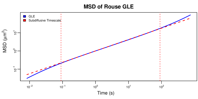
Figure 12: MSD of a Rouse GLE with $K=300$ and $\gamma=1.67$, $\tau=0.01$, $\nu=1$ (solid blue line). Also displayed is the subdiffusion timescale $(t_{\textnormal{min}},t_{\textnormal{max}})$ along with the power law $\operatorname{\textsc{msd}}_{X}(t)=2D_{\textnormal{eff}}\cdot t^{\alpha_{\textnormal{eff}}}$ on that range (red dotted lines).

Figure 12 also displays the subdiffusion timescale $(t_{\textnormal{min}},t_{\textnormal{max}})$ along with the power law $\operatorname{\textsc{msd}}_{X}(t)=2D_{\textnormal{eff}}\cdot t^{\alpha_{\textnormal{eff}}}$ on that range. The values of $(t_{\textnormal{min}},t_{\textnormal{max}},\alpha_{\textnormal{eff}},D_{\textnormal{eff}})$ are determined from the GLE parameters $K$ and ${\bm{\varphi}}=(\gamma,\tau,\nu)$ via the following method.

1. Calculate $x_{n}=\log(t_{n})$ and $y_{n}=\log\operatorname{\textsc{msd}}_{X}(t_{n}\mid{\bm{\varphi}},K)$ on a range of time points $t_{0},\ldots,t_{N}$. These should be picked on a fine grid such that $t_{0}\ll t_{\textnormal{min}}$ and $t_{N}\gg t_{\textnormal{max}}$.

2. Let $\bm{\Upsilon}=(t_{\textnormal{min}},t_{\textnormal{max}})$, and let $I_{\bm{\Upsilon}}=\{n:t_{\textnormal{min}}<t_{n}<t_{\textnormal{max}}\}$. Then for any $\bm{\Upsilon}$ we calculate $\alpha_{\textnormal{eff}}^{(\bm{\Upsilon})}$ and $D_{\textnormal{eff}}^{(\bm{\Upsilon})}$ via least-squares:

   $$\alpha_{\textnormal{eff}}^{(\bm{\Upsilon})}=\frac{\sum_{n\in I_{\bm{\Upsilon}}}(y_{n}-\bar{y})(x_{n}-\bar{x})}{\sum_{n\in I_{\bm{\Upsilon}}}(x_{n}-\bar{x})^{2}},\qquad D_{\textnormal{eff}}^{(\bm{\Upsilon})}=\tfrac{1}{2}\exp(\bar{y}-\alpha_{\textnormal{eff}}^{(\bm{\Upsilon})}\bar{x}),$$ (D.3)

   where $\bar{x}=\frac{1}{|I_{\bm{\Upsilon}}|}\sum_{n\in I_{\bm{\Upsilon}}}x_{n}$ and $\bar{y}=\frac{1}{|I_{\bm{\Upsilon}}|}\sum_{n\in I_{\bm{\Upsilon}}}y_{n}$ are the corresponding averages over the indices in $I_{\bm{\Upsilon}}$.

3. The subdiffusion timescale $\bm{\Upsilon}$ is determined by solving the constrained optimization problem

   $$\operatorname*{arg\,max}_{\bm{\Upsilon}}|\log(t_{\textnormal{max}})-\log(t_{\textnormal{min}})|\\ \textnormal{subject to}\qquad\max_{n\in I_{\bm{\Upsilon}}}\left|\frac{\alpha_{\textnormal{eff}}^{(\bm{\Upsilon})}\cdot x_{n}+\log(2D_{\textnormal{eff}}^{(\bm{\Upsilon})})-y_{n}}{y_{n}}\right|<\kappa,$$

   where $\kappa$ is a tolerance for departure from a perfect power law over the subdiffusive range. In Figure 12 and the calculations of Section 4.2 we have used $\kappa=1\%$. This optimization problem can be solved in $\mathcal{O}(N^{2})$ steps by trying all combinations of $t_{\textnormal{min}}$ and $t_{\textnormal{max}}$ in the set $\{t_{0},\ldots,t_{N}\}$.

References

- Amblard et al. (1996) Amblard, F., Maggs, A.C., Yurke, B., Pargellis, A.N., and Leibler, S. (1996). “Subdiffusion and anomalous local viscoelasticity in actin networks.” Physical review letters, 77(21): 4470.
- Ammar and Gragg (1988) Ammar, G.S. and Gragg, W.B. (1988). “Superfast solution of real positive definite toeplitz systems.” SIAM Journal on Matrix Analysis and Applications, 9(1): 61–76.
- Ashley and Andersson (2015) Ashley, T.T. and Andersson, S.B. (2015). “Method for simultaneous localization and parameter estimation in particle tracking experiments.” Physical Review E, 92(5): 052707.
- Berglund (2010) Berglund, A.J. (2010). “Statistics of camera-based single-particle tracking.” Physical Review E, 82(1): 011917.
- Brockwell and Davis (1991) Brockwell, P.J. and Davis, R.A. (1991). Time Series: Theory and Methods. Springer-Verlag, New York.
- Bronstein et al. (2009) Bronstein, I., Israel, Y., Kepten, E., Mai, S., Shav-Tal, Y., Barkai, E., and Garini, Y. (2009). “Transient anomalous diffusion of telomeres in the nucleus of mammalian cells.” Physical review letters, 103(1): 018102.
- Burov et al. (2017) Burov, S., Figliozzi, P., Lin, B., Rice, S.A., Scherer, N.F., and Dinner, A.R. (2017). “Single-pixel interior filling function approach for detecting and correcting errors in particle tracking.” Proceedings of the National Academy of Sciences, 114(2): 221–226.
- Calderon (2016) Calderon, C.P. (2016). “Motion blur filtering: A statistical approach for extracting confinement forces and diffusivity from a single blurred trajectory.” Physical Review E, 93(5): 053303.
- Chenouard et al. (2014) Chenouard, N., Smal, I., de Chaumont, F., Maška, M., Sbalzarini, I.F., Gong, Y., Cardinale, J., Carthel, C., Coraluppi, S., Winter, M., Cohen, A.R., Godinez, W.J., Rohr, K., Kalaidzidis, Y., Liang, L., Duncan, J., Shen, H., Xu, Y., Magnusson, K.E.G., Jaldén, J., Blau, H.M., Paul-Gilloteaux, P., Roudot, P., Kervrann, C., Waharte, F., Tinevez, J.Y., Shorte, S.L., Willemse, J., Celler, K., van Wezel, G.P., Dan, H.W., Tsai, Y.S., Ortiz de Solórzano, C., Olivo-Marin, J.C., and Meijering, E. (2014). “Objective comparison of particle tracking methods.” Nature methods, 11(3): 281.
- CISMM (2019a) CISMM (2019a). “Camera panoptes.” http://cismm.web.unc.edu/core-projects/force-microscopy/high-throughput-microscopy.
- CISMM (2019b) CISMM (2019b). “Video spot tracker.” http://cismm.web.unc.edu/resources/software-manuals/video-spot-tracker-manual.
- Claeskens and Hjort (2003) Claeskens, G. and Hjort, N.L. (2003). “The focused information criterion.” Journal of the American Statistical Association, 98(464): 900–916.
- Deschout et al. (2014) Deschout, H., Zanacchi, F.C., Mlodzianoski, M., Diaspro, A., Bewersdorf, J., Hess, S.T., and Braeckmans, K. (2014). “Precisely and accurately localizing single emitters in fluorescence microscopy.” Nature methods, 11(3): 253.
- Durbin (1960) Durbin, J. (1960). “The fitting of time series models.” Review of the International Statistical Institute, 28: 233 – 243.
- Edward (1970) Edward, J.T. (1970). “Molecular volumes and the stokes-einstein equation.” Journal of Chemical Education, 47(4): 261.
- Einstein (1956) Einstein, A. (1956). Investigations on the Theory of the Brownian Movement. Courier Corporation.
- Ernst et al. (2017) Ernst, M., John, T., Guenther, M., Wagner, C., Schaefer, U.F., and Lehr, C.M. (2017). “A model for the transient subdiffusive behavior of particles in mucus.” Biophysical Journal, 112(1): 172–179.
- Ferry (1980) Ferry, J.D. (1980). Viscoelastic properties of polymers. John Wiley & Sons.
- FLIR (2019) FLIR (2019). “Camera flear usb3.0.” https://www.ptgrey.com/products/flea3-usb3.
- Fong et al. (2013) Fong, E.J., Sharma, Y., Fallica, B., Tierney, D.B., Fortune, S.M., and Zaman, M.H. (2013). “Decoupling directed and passive motion in dynamic systems: particle tracking microrheology of sputum.” Annals of biomedical engineering, 41(4): 837–846.
- Freedman (2006) Freedman, D.A. (2006). “On the so-called “huber sandwich estimator” and “robust standard errors”.” The American Statistician, 60(4): 299–302.
- Gal et al. (2013) Gal, N., Lechtman-Goldstein, D., and Weihs, D. (2013). “Particle tracking in living cells: A review of the mean square displacement method and beyond.” Rheologica Acta, 52(5): 425–443.
- Grønneberg and Hjort (2014) Grønneberg, S. and Hjort, N.L. (2014). “The copula information criteria.” Scandinavian Journal of Statistics, 41(2): 436–459.
- Hermansen et al. (2015) Hermansen, G.H., Hjort, N.L., and Jullum, M. (2015). “Parametric or nonparametric: The fic approach for stationary time series.” In F.J. Samaniego, editor, Proceedings of the 60th World Statistics Congress of the International Statistical Institute, pages 4827–4832. The International Statistical Institute.
- Hill et al. (2014a) Hill, D.B., Vasquez, P.A., Mellnik, J., McKinley, S.A., Vose, A., Mu, F., Henderson, A.G., Donaldson, S.H., Alexis, N.E., Boucher, R.C. et al. (2014a). “A biophysical basis for mucus solids concentration as a candidate biomarker for airways disease.” PloS one, 9(2): e87681.
- Hill et al. (2014b) Hill, D.B., Vasquez, P.A., Mellnik, J., McKinley, S.A., Vose, A., Mu, F., Henderson, A.G., Donaldson, S.H., Alexis, N.E., Boucher, R.C. et al. (2014b). “A biophysical basis for mucus solids concentration as a candidate biomarker for airways disease.” PloS one, 9(2): e87681.
- Kailath et al. (1979) Kailath, T., Kung, S.Y., and Morf, M. (1979). “Displacement ranks of matrices and linear equations.” Journal of Mathematical Analysis and Applications, 68(2): 395–407.
- Kailath and Sayed (1999) Kailath, T. and Sayed, A.H., editors (1999). Fast Reliable Algorithms for Matrices with Structure. Society for Industrial and Applied Mathematics, Philadelphia.
- Koslover et al. (2016) Koslover, E.F., Chan, C.K., and Theriot, J.A. (2016). “Disentangling random motion and flow in a complex medium.” Biophysical journal, 110(3): 700–709.
- Kou (2008) Kou, S.C. (2008). “Stochastic modeling in nanoscale biophysics: subdiffusion within proteins.” The Annals of Applied Statistics, 2(2): 501–535.
- Kowalczyk et al. (2014) Kowalczyk, A., Oelschlaeger, C., and Willenbacher, N. (2014). “Tracking errors in 2d multiple particle tracking microrheology.” Measurement Science and Technology, 26(1): 015302.
- Kubo (1966) Kubo, R. (1966). “The fluctutation-dissipation theorem.” Reports on Progress in Physics, 29: 255–284.
- Lai et al. (2007) Lai, S.K., O’Hanlon, D.E., Harrold, S., Man, S.T., Wang, Y.Y., Cone, R., and Hanes, J. (2007). “Rapid transport of large polymeric nanoparticles in fresh undiluted human mucus.” Proceedings of the National Academy of Sciences, 104(5): 1482–1487.
- Lee et al. (2007) Lee, S.H., Roichman, Y., Yi, G.R., Kim, S.H., Yang, S.M., Van Blaaderen, A., Van Oostrum, P., and Grier, D.G. (2007). “Characterizing and tracking single colloidal particles with video holographic microscopy.” Optics Express, 15(26): 18275–18282.
- Levinson (1947) Levinson, N. (1947). “The Wiener RMS error criterion in filter design and prediction.” Journal Of Mathematical Physics, 25: 261 – 278.
- Ling and Lysy (2017) Ling, Y. and Lysy, M. (2017). SuperGauss: Superfast Likelihood Inference for Stationary Gaussian Time Series. URL https://CRAN.R-project.org/package=SuperGauss. R package version 1.0.
- Lysy et al. (2016) Lysy, M., Pillai, N.S., Hill, D.B., Forest, M.G., Mellnik, J.W., Vasquez, P.A., and McKinley, S.A. (2016). “Model comparison and assessment for single particle tracking in biological fluids.” Journal of the American Statistical Association, 111(516): 1413–1426.
- Mason et al. (1997) Mason, T., Ganesan, K., Van Zanten, J., Wirtz, D., and Kuo, S. (1997). “Particle tracking microrheology of complex fluids.” Physical Review Letters, 79(17): 3282.
- Mason and Weitz (1995) Mason, T.G. and Weitz, D. (1995). “Optical measurements of frequency-dependent linear viscoelastic moduli of complex fluids.” Physical review letters, 74(7): 1250.
- McKinley et al. (2009) McKinley, S.A., Yao, L., and Forest, M.G. (2009). “Transient anomalous diffusion of tracer particles in soft matter.” Journal of Rheology, 53(6): 1487–1506.
- Mellnik et al. (2016) Mellnik, J.W., Lysy, M., Vasquez, P.A., Pillai, N.S., Hill, D.B., Cribb, J., McKinley, S.A., and Forest, M.G. (2016). “Maximum likelihood estimation for single particle, passive microrheology data with drift.” Journal of Rheology, 60(3): 379–392.
- Michalet (2010) Michalet, X. (2010). “Mean square displacement analysis of single-particle trajectories with localization error: Brownian motion in an isotropic medium.” Physical Review E, 82(4): 041914.
- Michalet and Berglund (2012) Michalet, X. and Berglund, A.J. (2012). “Optimal diffusion coefficient estimation in single-particle tracking.” Physical Review E, 85(6): 061916.
- Mortensen et al. (2010) Mortensen, K.I., Churchman, L.S., Spudich, J.A., and Flyvbjerg, H. (2010). “Optimized localization analysis for single-molecule tracking and super-resolution microscopy.” Nature methods, 7(5): 377.
- Newby et al. (2018) Newby, J.M., Schaefer, A.M., Lee, P.T., Forest, M.G., and Lai, S.K. (2018). “Convolutional neural networks automate detection for tracking of submicron-scale particles in 2d and 3d.” Proceedings of the National Academy of Sciences, 115(36): 9026–9031.
- Qian et al. (1991) Qian, H., Sheetz, M.P., and Elson, E.L. (1991). “Single particle tracking. analysis of diffusion and flow in two-dimensional systems.” Biophysical journal, 60(4): 910–921.
- Rowlands and So (2013) Rowlands, C.J. and So, P.T. (2013). “On the correction of errors in some multiple particle tracking experiments.” Applied physics letters, 102(2): 021913.
- Savin and Doyle (2005) Savin, T. and Doyle, P.S. (2005). “Static and dynamic errors in particle tracking microrheology.” Biophysical journal, 88(1): 623–638.
- Saxton and Jacobson (1997) Saxton, M.J. and Jacobson, K. (1997). “Single-particle tracking: applications to membrane dynamics.” Annual review of biophysics and biomolecular structure, 26(1): 373–399.
- Sikora et al. (2017) Sikora, G., Teuerle, M., Wyłomańska, A., and Grebenkov, D. (2017). “Statistical properties of the anomalous scaling exponent estimator based on time-averaged mean-square displacement.” Physical Review E, 96(2): 022132.
- Soussou et al. (1970) Soussou, J., Moavenzadeh, F., and Gradowczyk, M. (1970). “Application of prony series to linear viscoelasticity.” Transactions of the Society of Rheology, 14(4): 573–584.
- Suh et al. (2005) Suh, J., Dawson, M., and Hanes, J. (2005). “Real-time multiple-particle tracking: applications to drug and gene delivery.” Advanced drug delivery reviews, 57(1): 63–78.
- Szymanski and Weiss (2009) Szymanski, J. and Weiss, M. (2009). “Elucidating the origin of anomalous diffusion in crowded fluids.” Physical review letters, 103(3): 038102.
- van der Schaar et al. (2008) van der Schaar, H.M., Rust, M.J., Chen, C., van der Ende-Metselaar, H., Wilschut, J., Zhuang, X., and Smit, J.M. (2008). “Dissecting the cell entry pathway of dengue virus by single-particle tracking in living cells.” PLoS pathogens, 4(12): e1000244.
- Varin et al. (2011) Varin, C., Reid, N., and Firth, D. (2011). “An overview of composite likelihood methods.” Statistica Sinica, pages 5–42.
- Vestergaard et al. (2014) Vestergaard, C.L., Blainey, P.C., and Flyvbjerg, H. (2014). “Optimal estimation of diffusion coefficients from single-particle trajectories.” Physical Review E, 89(2): 022726.
- Wang et al. (2008) Wang, Y.Y., Lai, S.K., Suk, J.S., Pace, A., Cone, R., and Hanes, J. (2008). “Addressing the peg mucoadhesivity paradox to engineer nanoparticles that “slip” through the human mucus barrier.” Angewandte Chemie International Edition, 47(50): 9726–9729.
- Weihs et al. (2007) Weihs, D., Teitell, M.A., and Mason, T.G. (2007). “Simulations of complex particle transport in heterogeneous active liquids.” Microfluidics and Nanofluidics, 3(2): 227–237.
- Weiss (2013) Weiss, M. (2013). “Single-particle tracking data reveal anticorrelated fractional brownian motion in crowded fluids.” Physical Review E, 88(1): 010101.
- Weiss et al. (2004) Weiss, M., Elsner, M., Kartberg, F., and Nilsson, T. (2004). “Anomalous subdiffusion is a measure for cytoplasmic crowding in living cells.” Biophysical journal, 87(5): 3518–3524.
- Wirtz (2009) Wirtz, D. (2009). “Particle-tracking microrheology of living cells: principles and applications.” Annual review of biophysics, 38: 301–326.
- Wong et al. (2004) Wong, I., Gardel, M., Reichman, D., Weeks, E.R., Valentine, M., Bausch, A., and Weitz, D.A. (2004). “Anomalous diffusion probes microstructure dynamics of entangled f-actin networks.” Physical review letters, 92(17): 178101.
- Working et al. (1997) Working, P.K., Newman, M.S., Johnson, J., and Cornacoff, J.B. (1997). “Safety of poly (ethylene glycol) and poly (ethylene glycol) derivatives.” ACS Publications.
- Zwanzig (2001) Zwanzig, R. (2001). Nonequilibrium Statistical Mechanics. New York: Oxford University Press.