A Bayesian/Information Theoretic Model of Bias Learning

Abstract

In this paper the problem of learning appropriate bias for an environment of related tasks is examined from a Bayesian perspective. The environment of related tasks is shown to be naturally modelled by the concept of an objective prior distribution. Sampling from the objective prior corresponds to sampling different learning tasks from the environment. It is argued that for many common machine learning problems, although we don’t know the true (objective) prior for the problem, we do have some idea of a set of possible priors to which the true prior belongs. It is shown that under these circumstances a learner can use Bayesian inference to learn the true prior by sampling from the objective prior. Bounds are given on the amount of information required to learn a task when it is simultaneously learnt with several other tasks. The bounds show that if the learner has little knowledge of the true prior, and the dimensionality of the true prior is small, then sampling multiple tasks is highly advantageous.

1 Introduction

In the VC and PAC models of learning [18, 17, 16], and indeed in most practical learning scenarios, the learner’s bias is represented by the choice of hypothesis space. This choice is extremely important: if the space is too large the learner will not be able to generalise well; if the space is too small it is unlikely to contain a solution to the problem being learnt.

A desirable goal in machine learning is to find ways of automatically learning appropriate bias, rather than having to build the bias in by hand. In the VC context this means finding ways of automatically learning the hypothesis space. A VC-type model of bias learning in the context of learning internal representations was introduced in [4], while a more general model that allows for any kind of specification of the hypothesis space is given in [3]. The central assumption of the model is that the learner is embedded within an environment of related tasks. The learner is able to sample from the environment and hence generate multiple data sets corresponding to different tasks. The learner can then search for a hypothesis space that is appropriate for learning all the tasks. This model can be thought of as a first order approximation to the idea that when choosing an appropriate hypothesis space or model for a learning problem, we are doing so on the basis of experience of similar problems.

It is shown in [4, 3] that under certain mild restrictions on the set of all hypotheisis spaces available to the learner, it is possible for the learner to sample sufficiently often from sufficiently many tasks to ensure that a hypothesis space containing hypotheses with small empirical loss on all the tasks will with high probability contain good solutions to novel tasks drawn from the same environment. It is also shown in those papers that if the learner is learning a common internal representation or preprocessing for an $n$ task training set (see figure 1) then the number of examples $m$ required of each task to ensure good generalisation obeys

$$m=O\left(a+\frac{b}{n}\right).$$ (1)

Here $a$ is a measure of the dimension of the smallest hypothesis space needed to learn all the tasks in the environment and $b$ is a measure of the dimension of the space of possible preprocessings available to the learner. The $n=1$ case of formula (1) is an upper bound the number of examples that would be required for good generalisation in the ordinary, single task learning scenario, while the limiting case of $m=O(a)$ is an upper bound on the number of examples required if the correct preprocessing is already known. Thus, this formula shows that the upper bound on the number of examples required per task for good generalisation decays to the minimal possible as the number of tasks being learnt increases.

Although very suggestive, without a matching lower bound of the same form, we cannot actually conclude from (1) that learning multiple related tasks requires fewer examples per task for good generalisation than if those tasks are learnt independently. Unfortunately, lower bounds within a real-valued VC/PAC framework are in general very difficult to come by because an infinite amout of information can be conveyed in a single real value and so it is possible to construct complicated function classes in which the identity of each function is encoded in its value at every point (see e.g. [2]). This suggests that rather calculating the number of examples required to learn, we should calculate the amount of information required to learn.

In this paper the model of bias learning introduced in [4] and [3] is modified to a Bayesian model of bias learning. There are a number of reasons for this. One is that the question “how much information is required to learn” is more natural within a Bayesian model than within the VC model. Another reason is that it is much easier to formulate and analyse the effects of prior knowledge on the learning process. This is particularly important in bias learning where we are trying to understand how the process of aquiring prior knowledge can be automated. In the VC framework the learner’s prior knowledge is represented by the hypothesis space chosen for the problem. All hypotheses within the hypothesis space are viewed equally, whereas in the Bayesian framework the learner can rank the hypotheses in order of prior preference using a prior distribution. In addition, the Bayesian learner does not have to choose a particular hypothesis as the result of the learning process, it simply ranks the alternative hypotheses in the light of the data. Finally, quantities involving information (in the Shannon sense) have a more natural expression within a Bayesian framework.

The main feature of the Bayesian bias learning model introduced here is that the prior is treated as objective. The sample space of the prior represents the space of tasks in the environment, and sampling from the prior corresponds to selecting different learning tasks from the environment. The analagous question to “how many examples are required of each task in an $n$ task training set” leading to the upper bound (1), is “how much information is required per task to learn $n$ tasks?” We will see that if the learner already knows the true prior then there is no advantage to learning $n$ tasks; that is, the expected amount of information needed to learn each task within an $n$ task training set is the same as if the tasks are learnt separately. However, if the learner does not know the true prior (which is generally the case in bias learning, otherwise there is no need to do bias learning), but instead knows only that the prior is one of a set $\Pi$ of possible priors (the possible priors in this case correspond to the different hypothesis spaces available to the learner in the VC/PAC model of bias learning), then we will see that the expected information needed per task, ${\overline{R}}_{n,\pi^{*}}$, obeys asymptotically (in $n$)

$${\overline{R}}_{n,\pi^{*}}\doteq a^{\prime}+b^{\prime}(\pi^{*})\frac{\log n}{n}+o\left(\frac{\log n}{n}\right)$$ (2)

where $a^{\prime}$ is the minimal amount of information possible (the amount the learner would require if it knew the true prior $\pi^{*}$) and $b^{\prime}(\pi^{*})$ is a local measure of the dimension of the space of possible priors $\Pi$ at the point $\pi^{*}$. Here $f(n,\pi^{*})\doteq g(n,\pi^{*})$ means $f(n,\pi)=g(n,\pi)$ for all but a set of $\pi$ of vanishingly small measure as $n\rightarrow\infty$. Comparing (2) and (1) and the meaning of $a$ and $b$ with their partners $a^{\prime}$ and $b^{\prime}$, we see that this partially realises the aim of providing an exact bound justifying learning multiple related tasks.

The question of how much information is required to encode the $m$’th observation of each task in an $n$ task training set is also analysed in this paper, and an example is given showing that when the true prior is unknown, learning multiple tasks is also highly advantageous in this setting.

The rest of the paper is organised as follows. The Bayesian model of bias learning is introduced formally in section 2, along with a concrete example based on neural networks for image recognition. The relationship between Bayesian bias learning as formulated here and hierarchical Bayesian methods is also discussed. Equation (2) is derived in section 3 and the constants $a$ and $b$ are calculated for the neural network example, where again contact is made between the Bayesian model results and the VC model results. In section 4 the question of how much information is required to encode the $m$’th observation of each task in an $n$ task training set is analysed. In section 4.1 the dimension of a fairly general class of smoothly parameterised models is calculated, leading to a characterisation of the advantages of multiple task learning within a Bayesian context.

1.1 Notation

The probability model treated throughtout this paper is three-tiered. At the bottom level is $Z$ which is assumed to be a complete separable metric space. All probability measures on $Z$ are defined on the sigma-field of Borel subsets of $Z$. $Z$ is the learner’s interface with the environment—the learner receives all its data in the form of samples from $Z$. The next level up in the hierarchy is $\Theta$, which is the set of possible “states of nature” or “learning tasks” with which the learner might be confronted. For each $\theta\in\Theta$ there is a probability measure $P_{Z|\theta}$ on $Z$. We assume there exists a fixed $\sigma$-finite measure $\nu$ that dominates $P_{Z|\theta}$ for each $\theta\in\Theta$. $\Theta$ is also assumed to be a complete separable metric space. At the highest level in the hierarchy is the set $\Pi$ which represents the space of possible “priors” on $\Theta$. For each $\pi\in\Pi$ there is a probability measure $P_{\Theta|\pi}$ on $\Theta$. Again the $P_{\Theta|\pi}$’s are defined on the sigma field of Borel subsets of $\Theta$ and we assume there exists a second measure $\mu$ dominating all $P_{\Theta|\pi}$. Finally, on $\Pi$ there is a fixed probability measure $P_{\Pi}$: the “hyper-prior”. As $\Theta$ is a complete separable metric space, we can take the domain of $P_{\Pi}$ to be the sigma field generated by the topology of weak convergence of the $P_{\Theta|\pi}$ measures.

Integration with respect to the measures $\nu$ and $\mu$ will be denoted by $\int_{Z}\,dz$ and $\int_{\Theta}\,d\theta$ respectively ($\nu$ and $\mu$ are not assumed to be Lebesgue measures—the notation is just for convenience). Integration with respect to the hyper-prior $P_{\Pi}$ will be denoted $\int_{\Pi}p(\pi)\,d\pi$ The Radon-Nikodym derivative of any measure $P_{Z|\theta}$ at $z\in Z$, $\frac{dP_{Z|\theta}}{d\nu}(z)$ will be written interchangably as $p(z|\theta)$ or $p_{Z|\theta}(z)$, and similarly $\frac{dP_{\Theta|\pi}}{d\mu}(\theta)$ will be written as $p(\theta|\pi)$ or $p_{\Theta|\pi}(\theta)$.

If $f$ is a function on $Z$, then the expectation of $f$ with respect to any random variable with distribution $P_{Z|\theta}$ will be denoted by $\mathbb{E}_{Z|\theta}f(z)=\int_{Z}f(z)p(z|\theta)\,dz$. Similarly for functions defined on $\Theta$ and $\Pi$.

$n\times m$ matrices with elements from $Z$ will be denoted by $\bf z$:

$${\mbox{\boldmath$\bf z$}}=\begin{matrix}z_{11}&\ldots&z_{1m}\\ \vdots&\ddots&\vdots\\ z_{n1}&\ldots&z_{nm}.\end{matrix}$$

The columns of $\bf z$ will be denoted as $z^{n}_{i}$, so ${\mbox{\boldmath$\bf z$}}=[z^{n}_{1}\dots z^{n}_{m}]$.

Let ${\cal N}$ denote the natural numbers.

2 The Basic Model

In Bayesian models of learning (see e.g. [6]) the learner recieves data $z^{n}=z_{1},\dots,z_{n}$ which are observations on $n$ random variables $Z^{n}=Z_{1},\dots,Z_{n}$. The $Z_{i}$ are identically distributed and conditionally independent given the true state of nature $\theta$. The learner does not know $\theta$, but does know that $\theta$ belongs to a set of possible states of nature $\Theta$. The learner begins with a prior distribution $p(\theta)$ and upon receipt of the data $z^{n}$ updates $p(\theta)$ to a posterior distribution $p(\theta|z^{n})$ according to Bayes’ rule:

$$p(\theta|z^{n})=\frac{p(z^{n}|\theta)p(\theta)}{p(z^{n})},$$ (3)

where

$$p(z^{n})=\int_{\Theta}p(z^{n}|\theta)p(\theta)\,d\theta.$$

Bayesian approaches to neural network learning have been around for a while (see e.g. [13]), and they essentially constitute a subset of Bayesian approaches to non-linear regression and classification. Mapping these approaches on to the present framework, consider the case of an MLP for recognising my face. The weights of the network correspond to the set of possible states of nature $\Theta$, the true state of nature $\theta^{*}$ being an assignment of weights such that the output of the network is 1 when an example of my face is applied to its input, and 0 if anything else is applied to its input. The data $z^{n}=z_{1},\dots,z_{n}$ comes in the form of input-output pairs $z_{i}=(x_{i},y_{i})$ where each $x_{i}$ is an example image and $y_{i}$ is the correct class label (in this case either 0 or 1). Note that as we are only interested in classification in this example, the input distribution $p(x)$ is not modelled, only the conditional distribution on class labels $p(y|x)$. Denoting the output of the network by $f_{\theta}(x)$, and interpreting $f_{\theta}(x)$ as $p(y=1|x)$, it can easily be shown [7] that the probability of data set $z^{n}=(x_{1},y_{1}),\dots,(x_{n},y_{n})$ given weights $\theta$ is

$$p(z^{n}|\theta)=\prod_{i=1}^{n}p(x_{i})e^{-E(z^{n};\theta)}$$ (4)

where

$$E(z^{n};\theta)=\sum_{i=1}^{n}y_{i}\log(f_{\theta}(x_{i}))+(1-y_{i})\log(f_{\theta}(x_{i})).$$

Choosing a prior (typically multivariate Gaussian or uniform over some compact set) for the weights and substituting (4) into (3) yields the posterior distribution on the weights $p(\theta|z^{n})$. The posterior is the “output” of the learning process. It can be used to predict the class label of a novel input $x^{*}$ by integrating:

$$p(y=1|x^{*};z^{n})=\int_{\Theta}f_{\theta}(x^{*})p(\theta|z^{n})\,d\theta.$$

2.1 Interpreting the Prior

In the example above the prior $p(\theta)$ is a purely subjective prior. As is typical for these problems a relatively weak prior is chosen reflecting our weak knowledge about appropriate weight settings for this problem. However, in the case of face recognition (and many other pattern recognition problems such as speech and character recognition) it is arguable that there exists an objective prior for the problem. To see this, note that given our weak prior knowledge we are likely to have chosen a network large enough to solve any face recogition problem within some margin of error, not just the specific task: “recognise Jon ”. Hence it is likely that there will exist weight settings $\theta_{1},\theta_{2},\theta_{3},\dots$ that will cause the network to behave as a classifier for ‘Mary’, ‘Joe’, ‘males’, ‘smiling’, ‘big nose’ and so on. In fact there should exist weight settings that correspond to nonexistent faces provided different examples of the face vary in a “face-like” way. Hence we can consider the space of all face classifiers, both real and fictitious, as represented by a particular subset $\Theta_{\text{face}}$ of all possible weight settings $\Theta$. The objective prior $p(\theta)$ for face recognition is then characterised by the fact that its support is restricted to $\Theta_{\text{face}}$. The restriction of the support is the most important aspect of the face prior. The actual numerical probabilities for each element $\theta\in\Theta_{\text{face}}$ could be chosen in a number of different ways, but for the sake of argument we can take them to be uniform or as corresponding to the general frequency of face-like classifier problems encountered in a particular person’s environment.

The usual subjective priors chosen in neural network applications (Gaussian or uniform on the weights) bear no resemblence to the objective prior discussed above: initializing the weights of a network according to a Gaussian prior typically does not cause the network to behave like some kind of face classifier, whereas initializing according to the objective prior by definition will induce such behaviour. Hence the use of subjective priors such as the Gaussian not only demonstrates our ignorance concerning the specific task at hand (e.g. learn to recognise Jon) but also demonstrates our ignorance concerning the true prior. That is, we typically have little idea which parameter settings $\theta$ correspond to face-like classifiers and which correspond to “random junk”.

Should we care that we don’t know the true prior? In short: yes. If we know the true prior then the task of learning any individual face is vastly simplified. A single positive example of my face is enough to set the posterior probability of any other individual face classifiers to zero (or very close to zero), and a few more examples with me smiling, frowning, bearded, clean-shaven, long-haired, short-haired and so on is enough to set the posterior probability of every other classifier (the smiling, frowning, etc classifiers) except the “Jon” classifier to zero. Contrast this with the usual subjective priors where typically thousands of examples and counter-examples of my face would have to be supplied to the network before a reasonably peaked posterior and hence reasonable generalisation could be achieved.

2.2 Learning the Prior

If knowing the true prior is such a great advantage then we should try to learn it. To do this we can set up a space of candidate priors indexed by some set $\Pi$. Thus, each $\pi\in\Pi$ corresponds to some prior $p(\theta|\pi)$ on $\Theta$. We assume realizability, so that the objective prior $p(\theta|\pi^{*})$ corresponds to some $\pi^{*}\in\Pi$. To complete the Bayesian picture a subjective prior $p(\pi)$ must be chosen for $\Pi$. Typically we will not have a strong preference for any particular prior and so we can follow the course taken in ordinary Bayesian inference under such circumstances and choose $p(\pi)$ to be non-informative or simply Gaussian with large variance or uniform over some compact set (assuming $\Pi$ is Euclidean).

As the true prior $p(\theta|\pi^{*})$ is objective we can in principle sample from it to generate a sequence of training tasks $\theta^{n}=\theta_{1},\theta_{2},\dots,\theta_{n}$. A direct application of Bayes’ rule then gives the posterior probability of each prior:

$$p(\pi|\theta^{n})=\frac{p(\theta^{n}|\pi)p(\pi)}{p(\theta^{n})}$$

where $p(\theta^{n}|\pi)=\prod_{i=1}^{n}p(\theta_{i}|\pi)$ and $p(\theta^{n})=\int_{\Pi}p(\theta^{n}|\pi)p(\pi)\,d\pi$.

Under appropriate conditions the posterior distribution will tend to a delta function over the true prior $\pi^{*}$ as $n\rightarrow\infty$. Thus for large enough $n$ the learner can be said to have learnt the prior.

For this model to work we have to assume that although the learner has no idea about the true prior, it can generate a class of priors $\Pi$ containing the true prior $\pi^{*}$. This assumption is quite reasonable in the case of face recognition because it seems plausible that there exists a low-dimensional internal representation for faces such that each face classifier can be implemented by a simple map (e.g. linear or nearest-neightbour) composed with the internal representation. A low dimensional representation (LDR) in its simplest form is just a fixed mapping from the (typically high-dimensional) input space to a much smaller dimensional space. One can think of the LDR as a preprocessing applied to the input data that extracts features that are important for classification. For example, in the case of face recognition it might be that to uniquely determine any face one only needs to know the distance between the eyes and the length of the nose. So an appropriate LDR would be a two-dimensional one that extracts these two features from an image. Although faces almost certainly cannot be represented solely by the inter-eye distance and nose length, it is highly plausible that some kind of LDR exists for the face recognition problem. It is similarly plausible that LDR’s exist for other pattern recognition problems such as character and speech recognition

Figure 1 illustrates how in the case of neural-network learning the assumption that there exists an LDR for the tasks in the environment can be translated into a specification for the set of possible priors $\Pi$. The hidden layers of the network labelled LDR correspond to the LDR, while each individual classifier task is assumed to be implementable by composing a linear map with the output of the LDR. Thus each $\theta\in\Theta$ divides into two parts: $\theta=(\theta_{\text{LDR}},\theta_{\text{OUT}})$, where $\theta_{\text{LDR}}$ are the hidden layer weights and $\theta_{\text{OUT}}$ are the weights of the linear output map. As a first approximation, it is reasonable to assume that the true prior $p(\theta|\pi^{*})$ is a delta function positioned at $\theta^{*}_{\text{LDR}}$—the true preprocessing (LDR), and fairly uniform over output layer weight settings. Hence it is reasonable to take $\Pi$ to be the set of all priors that are a delta function over some $\theta_{\text{LDR}}$, and fairly smooth Gaussians (or uniform distributions) over $\theta_{\text{OUT}}$. To simplify matters assume that the distribution on $\theta_{\text{OUT}}$ is the same for all priors. With these assumptions, $\Pi$, the set of possible priors of this form is isomorphic to the set of possible weights in the hidden layers, $\Theta_{\text{LDR}}$. In this model knowing the true prior is equivalent to knowing the correct input-hidden layer weights. Learning any individual task is then simply a matter of estimating the output weights for a single node which is a simple problem of linear regression. The output layer weights are thus the model parameters while the hidden layer weights are the model hyper-parameters.

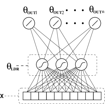
Figure 1: A neural network for low dimensional representation (LDR) learning. Each task in the environment is implemented by composing a linear map with weights $\theta_{{\text{\rm OUT}}i}$ with a fixed preprocessing or LDR. In the example considered in this paper the LDR is a single layer neural network with sigmoidal nodes. The weights of the LDR are $\theta_{\text{\rm LDR}}$. The $\theta_{\text{\rm LDR}}$ weights are hyper-parameters while the $\theta_{\text{\rm OUT}}$ weights are ordinary model parameters.

2.3 Relationship to hierarchical Bayes and existing Bayesian neural network techniques

The framework outlined in the previous section is in fact a special case of what is known as hierarchical Bayesian inference (see e.g [5, 6, 10]). Hierarchical Bayesian inference has also been discussed in the context of neural networks by several authors (see e.g. [13], although the techniques presented there are not explicitly identified by the author as hierarchical Bayes). The distinction between subjective and objective priors has been observed and the idea of multiple sampling from objective priors has been analysed for a number of different models. However the models analysed are typically quite low-dimensional in comparison to the kind of models used in neural network research. Will we see in the following section that Hierarchical Bayes with multiple task sampling can be particularly useful in high-dimensional models.

To the best of my knowledge the idea of an objective prior has not been employed previously in Bayesian approaches to neural networks. For the most part the hierarchical Bayes approach has been used to tune a small number of “nuisance” (hyper) parameters (such as the parameter $\lambda$ controlling the trade-off between regularisation and data-misfit in regression networks [14]). Note that these are the only parameters which are treated as hyper-parameters. All the network weights are treated as proper model parameters. However, as our previous discussion shows, in cases when there exists an environment of tasks posessing a common internal representation, the hidden layer weights of a neural network should be viewed as hyper-parameters, not model parameters. The only model parameters are the output weights. Thus, rather than the model parameters vastly outnumbering the hyperparameters, we have the opposite situation here with the hyper-parameters vastly outnumbering the model parameters. We will see in the remainder of this paper that such an arrangement of parameters is by far the most efficient, for two reasons. Firstly, once the hyperparameters have been learnt, i.e. the objective prior has been identified, then learning a novel task in the same environment requires only that the model parameters be learnt, which for models with a small number of parameters will be a relatively simple task and require few examples. Secondly, learning multiple tasks turns out be far more efficient when the hyper-parameters dominate the model parameters.

3 Learning Multiple Tasks

Having set up the model of Bayesian bias learning in the previous section, we can now tackle the question posed in the introduction: “How much information is required per task to learn $n$ tasks simultaneously?”

Note that if the learner already knows the true prior $p(\theta|\pi^{*})$, then the expected amount of information required per task to learn $n$ tasks is

$$\frac{H(P_{\Theta^{n}|\pi^{*}})}{n}=H(P_{\Theta|\pi^{*}})$$ (5)

because $P_{\Theta^{n}|\pi^{*}}=P_{\Theta|\pi^{*}}^{n}$ and entropy is additive over products of independent distributions (here $H(P_{\Theta|\pi^{*}})=-\mathbb{E}_{\Theta|\pi^{*}}\log p(\theta|\pi^{*})$ is the entropy of the true prior). As $H(P_{\Theta|\pi^{*}})$ is the expected amount of information required to learn a single task, we can see that there is no advantage to learning multiple tasks if the true prior is known.

If the true prior is unknown, but the learner is in posession of a family of priors $\Pi$, then the expected amount of information required per task to learn $n$ tasks is

$${\overline{R}}_{n,\pi^{*}}:=\frac{H_{\pi^{*}}(P_{\Theta^{n}})}{n},$$ (6)

where $H_{\pi^{*}}(P_{\Theta^{n}})=-\mathbb{E}_{\Theta^{n}|\pi^{*}}\log(p(\theta^{n}))$ where $p(\theta^{n})=\int_{\Pi}p(\theta^{n}|\pi)p(\pi)\,d\pi$ is the induced or mixture prior on $\theta^{n}$. Rather than tackling ${\overline{R}}_{n,\pi^{*}}$ directly it is more convenient to analyse the expected difference between the information required to learn $n$ tasks using the true prior $p(\theta^{n}|\pi^{*})$ and the information required to learn $n$ tasks using the induced prior $p(\theta^{n})$. This quantity is

$$\int_{\Theta^{n}}p(\theta^{n}|\pi^{*})\log\frac{p(\theta^{n}|\pi^{*})}{p(\theta^{n})}\,d\theta^{n}=D_{K}(P_{\Theta^{n}|\pi^{*}}\|P_{\Theta^{n}}),$$

which is the Kullback-Liebler divergence between the true and induced distributions on $\Theta^{n}$. Note that if we know $D_{K}(p_{\Theta^{n}|\pi^{*}}\|p_{\Theta^{n}})$ we can recover ${\overline{R}}_{n,\pi^{*}}$ from the relation

$${\overline{R}}_{n,\pi^{*}}=\frac{1}{n}D_{K}(P_{\Theta^{n}|\pi^{*}}\|P_{\Theta^{n}})+H(P_{\Theta|\pi^{*}})$$ (7)

To bound $D_{K}(P_{\Theta^{n}|\pi^{*}}\|P_{\Theta^{n}})$ the following definitions are needed.

Definition 1.

For any $\pi,\pi^{\prime}\in\Pi$, let $\Delta_{H}(\pi,\pi^{\prime})$ denote the squared Hellinger distance squared between the two priors $P_{\Theta|\pi}$ and $P_{\Theta|\pi^{\prime}}$:

$$\Delta_{H}(\pi,\pi^{\prime})=\int_{\Theta}\left[\sqrt{p(\theta|\pi)}-\sqrt{p(\theta|\pi^{\prime})}\right]^{2}\,d\theta$$

and let $\Delta_{K}(\pi,\pi^{\prime})$ denote the Kullback-Liebler divergence between the two priors $p(\theta|\pi),p(\theta|\pi^{\prime})$:

$$\Delta_{K}(\pi,\pi^{\prime})=\int_{\Theta}p(\theta|\pi)\log\frac{p(\theta|\pi)}{p(\theta|\pi^{\prime})}\,d\theta.$$

Let $B_{\varepsilon}(\pi)=\{\pi^{\prime}\colon\Delta^{1/2}_{H}(\pi,\pi^{\prime})\leq{\varepsilon}\}$, i.e. the Hellinger ball of radius ${\varepsilon}$ around $\pi$. For all $\pi\in\Pi$, define the local metric dimension of $\pi$ by

$$\dim_{P_{\Pi}}(\pi)=\lim_{{\varepsilon}\rightarrow 0}\frac{-\log P_{\Pi}(B_{\varepsilon}(\pi))}{\log\frac{1}{{\varepsilon}}}$$

whenever the limit exists ($P_{\Pi}$ is the subjective (hyper) prior probability distribution on $\Pi$).

Note that $(\Pi,\Delta^{1/2}_{H})$ is a metric space while $(\Pi,\Delta_{K})$ is not ($\Delta_{K}$ is asymmetric and does not satisfy the triangle inequality). Also, $\Delta_{K}(\pi,\pi^{\prime})\geq\frac{1}{2}\Delta_{H}(\pi,\pi^{\prime})$ always (see e.g. [11]).

Definition 2.

Let $(X,\Sigma,P)$ be a measure space and $f,g\colon{\cal N}\times X\to{\mathbb{R}}$ be two real-valued functions on ${\cal N}\times X$. We say

$$f(m,x)\doteq g(m,x)$$

if $\lim_{m\rightarrow\infty}P(X_{m})=1$ where for each $m\in{\cal N}$, $X_{m}=\{x\colon f(m,x)=g(m,x)\}$.

Theorem 1.

If there exists $\alpha<\infty$ such that for all $\pi,\pi^{\prime}\in\Pi$,

$$\Delta_{K}(\pi,\pi^{\prime})\leq\alpha\Delta_{H}(\pi,\pi^{\prime}),$$

and $\dim_{P_{\Pi}}(\pi)$ exists for all $\pi\in\Pi$, then

$$\frac{D_{K}(P_{\Theta^{n}|\pi^{*}}\|P_{\Theta^{n}})}{\log n}\doteq\frac{\dim_{P_{\Pi}}(\pi^{*})}{2}+o(1),$$ (8)

where $o(1)$ is a function of $m$ for which $\lim_{m\rightarrow\infty}o(1)(m)=0$.

Proof.  See section 6.
Note that if

$$\inf_{\pi,\pi^{*}\in\Pi\,{\text{and}}\,\theta\in\Theta}\frac{p(\theta|\pi)}{p(\theta|\pi^{*})}<\infty$$

then there exists $\alpha<\infty$ such that $\Delta_{K}(\pi,\pi^{\prime})\leq\alpha\Delta_{H}(\pi,\pi^{\prime})$ [11].

Theorem 2.

Under the same conditions as theorem 1,

$${\overline{R}}_{n,\pi^{*}}\doteq\frac{\dim_{P_{\Pi}}(\pi^{*})}{2}\frac{\log n}{n}+H(P_{\Theta|\pi^{*}})+o\left(\frac{\log n}{n}\right),$$

where $o\left(\log n/n\right)$ approaches zero faster than $\log n/n$ as $n\rightarrow\infty$.

Proof.  The theorem follows directly from (7) and theorem 1.
Note that this result is not quite as strong as it looks on face value because the set of priors for which

$${\overline{R}}_{n,\pi^{*}}=\frac{\dim_{P_{\Pi}}(\pi^{*})}{2}\frac{\log n}{n}+H(P_{\Theta|\pi^{*}})+o\left(\frac{\log n}{n}\right)$$ (9)

fails can vary with $n$, even though its measure becomes vanishingly small. This implies that for any individual $\pi^{*}\in\Pi$, (9) may fail for infinitely many $n$. However, if the sum over all $n$ of the $P_{\Pi}$ measure of the sets of $\pi^{*}$ for which (9) fails is finite, then by Borel-Cantelli, for all but a set of $\pi$ of $P_{\Pi}$ measure zero, (9) will fail only finitely often.

Setting $a=H(P_{\Theta|\pi^{*}})$ and $b=\frac{\dim_{P_{\Pi}}(\pi^{*})}{2}$, theorem 2 shows that the expected amount of information required per task to learn an $n$ task training set approaches

$$a+\frac{b\log n}{n},$$

except for a set of priors of vanishingly small measure as $n\rightarrow\infty$, which in turn approaches $a$—the minimum amount of information required to learn a task on average ($a$ is the amount of information required if the true prior is known, c.f. (5)).

3.1 Example: learning an LDR

Recall from section 2.2 that for the problem of learning a Low Dimensional Representation (LDR), $\Theta$ is split into $(\Theta_{\text{\rm LDR}},\Theta_{\text{\rm OUT}})$. We chose each prior $\pi\in\Pi$ to be delta function over some $\theta_{\text{\rm LDR}}$ and uniform or Gaussian over $\Theta_{\text{\rm OUT}}$. In order to apply the results of the previous section we need to smooth out the delta functions, otherwise the correct prior is identifiable from the observation of a single task $\theta$. So instead take the prior for each $\pi$ to be a Gaussian with small variance $\sigma_{\Pi}$ peaked over some $\theta_{\text{\rm LDR}}$. In addition, for $H(P_{\Theta|\pi})$ to be well defined the output weights $\theta_{\text{\rm OUT}}$ need to be quantized, so let each weight $w$ be coded with $k$ bits and take the distribution over the discretized $\Theta_{\text{\rm OUT}}$ to be uniform for each prior $\pi$. Denote the number of weights in $\Theta_{\text{\rm LDR}}$ by $W_{\text{\rm LDR}}$ and the number of weights in $\Theta_{\text{\rm OUT}}$ by $W_{\text{\rm OUT}}$. For any $\pi\in\Pi$, let $\theta_{\text{\rm LDR}}(\pi)$ denote the mean of the distribution $p(\theta_{\text{\rm LDR}}|\pi)$. Finally, take the prior distribution on $\Pi$ to be uniform over some compact subset of $\Theta_{\text{\rm LDR}}$.

A simple calculation shows the Hellinger and Kullback-Liebler distances to be given by

$$\Delta_{H}(\pi,\pi^{\prime}) =2\left(1-e^{\frac{1}{8\sigma_{\Pi}^{2}}\|\theta_{\text{\rm LDR}}(\pi)-\theta_{\text{\rm LDR}}(\pi^{\prime})\|^{2}}\right),$$

$$\Delta_{K}(\pi,\pi^{\prime}) =\frac{1}{2\sigma_{\Pi}^{2}}\|\theta_{\text{\rm LDR}}(\pi)-\theta_{\text{\rm LDR}}(\pi^{\prime})\|^{2}$$

Note that as $\Delta_{H}(\pi,\pi^{\prime})\rightarrow 0$, $\Delta_{H}(\pi,\pi^{\prime})\rightarrow\frac{1}{4\sigma_{\Pi}^{2}}\|\theta_{\text{\rm LDR}}(\pi)-\theta_{\text{\rm LDR}}(\pi^{\prime})\|^{2}$. Substituting this expression into the definition of $\dim_{P_{\Pi}}(\pi)$ we find

$$\dim_{P_{\Pi}}(\pi)=W_{{\text{\rm LDR}}}$$

for all $\pi\in\Pi$. Trivially, $H(P_{\Theta|\pi})=kW_{\text{\rm OUT}}$ for all $\pi\in\Pi$. The fact that the prior on $\Pi$ is compactly supported coupled with the use of a Gaussian prior on $\Theta$ ensures that $\Delta_{K}(\pi,\pi^{\prime})$ is bounded above by $\alpha\Delta_{H}(\pi,\pi^{\prime})$ for all $\pi,\pi^{\prime}$ and some $\alpha<\infty$. Hence the conditions of theorem 2 are satisified and we have

$${\overline{R}}_{n,\pi^{*}}\doteq\frac{W_{\text{\rm LDR}}}{2}\frac{\log n}{n}+kW_{\text{\rm OUT}}+o\left(\frac{\log n}{n}\right).$$

The similarity of this expression to the upper bound on the number of examples required per task for good generalisation in a PAC sense of $O(W_{\text{\rm OUT}}+W_{\text{\rm LDR}}/n)$ is noteworthy (see [4] for a derivation of the latter expression).

4 Sampling multiple tasks

Theorem 2 was derived under the assumption that the learner receives information about the tasks $\theta$ directly. In fact ${\overline{R}}_{n,\pi^{*}}$ is (within one query) the average number of queries the learner will require to identify a task in an $n$-task training set if the queries are restricted to be of the form “is $\theta\in A$” where $A$ is any subset of $\Theta$ and the learner uses the best possible querying strategy.

In general the learner will not be able to query in this way, but instead will receive information about the parameters $\theta$ indirectly via a sample $z^{m}=(z_{1},\dots,z_{m})$, sampled i.i.d. according to $p(z|\theta)$. If the learner is learning $n$ tasks simultaneously then it will recieve $n$ such samples (called an (n,m)-sample in [4, 3]):

$${\mbox{\boldmath$\bf z$}}=\begin{matrix}z_{11}&\ldots&z_{1m}\\ \vdots&\ddots&\vdots\\ z_{n1}&\ldots&z_{nm}\end{matrix}$$

Let ${Z^{(n,m)}}$ denote the set of all such ${z^{(n,m)}}$. The correct hierarchical Bayes approach to learning the $n$ tasks $\theta_{1},\dots,\theta_{n}$ is to use the hyper prior $P_{\Pi}$ to generate a prior distribution on $\Theta^{n}$ via

$$p(\theta^{n}) =\int_{\Pi}p(\theta^{n}|\pi)p(\pi)\,d\pi$$

$$=\int_{\Pi}p(\pi)\prod_{i=1}^{n}p(\theta_{i}|\pi)\,d\pi$$

and then the posterior $p(\theta^{n}|{\mbox{\boldmath$\bf z$}})$ can be computed in the usual way

$$p(\theta^{n}|{\mbox{\boldmath$\bf z$}}) =\frac{p({\mbox{\boldmath$\bf z$}}|\theta^{n})p(\theta^{n})}{p({\mbox{\boldmath$\bf z$}})}$$ (10)

$$=\frac{p(\theta^{n})\prod_{i=1}^{n}\prod_{j=1}^{m}p(z_{ij}|\theta_{i})}{p({\mbox{\boldmath$\bf z$}})}$$ (11)

where $p({\mbox{\boldmath$\bf z$}})=\int_{\Theta^{n}}p(\theta^{n})\prod_{i=1}^{n}\prod_{j=1}^{m}p(z_{ij}|\theta_{i})\,d\theta^{n}$.

One way to measure the advantage in learning $n$ tasks together is by the rate at which the learner’s loss in predicting novel examples decays for each task. In keeping with our philosophy of measuring loss in information terms (i.e. via relative entropy), the expected loss per task of the learner when predicting the $m+1$th observation of each task, $z^{n}_{m+1}$, after receiving $\bf z$, is

$${\overline{R}}_{n,m,\pi^{*}}=\frac{1}{n}\mathbb{E}_{\Theta^{n}|\pi^{*}}\mathbb{E}_{{Z^{(n,m)}}|\theta^{n}}\mathbb{E}_{{Z^{n}}|\theta^{n}}\log\frac{p(z^{n}|\theta^{n})}{p(z^{n}|{\mbox{\boldmath$\bf z$}})},$$ (12)

where $p(z^{n}|{\mbox{\boldmath$\bf z$}})$ is the learner’s predictive distribution on ${Z^{n}}$ based on the information contained in $\bf z$ and is given by

$$p(z^{n}|{\mbox{\boldmath$\bf z$}})=\int_{\Theta^{n}}p(z^{n}|\theta^{n})p(\theta^{n}|{z^{(n,m)}})\,d\theta^{n}.$$

where $p(\theta^{n}|{z^{(n,m)}})$ is computed via (10). Note that (12) is also the expected loss of a learner that has first received $m$ observations of $n$ tasks, $\bf z$, then observed $m$ observations of a new task, and is predicting the $m+1$th observation the new task. In this way it is a measure of the extent to which the learner has learnt to learn the tasks in the environment after receiving $\bf z$.

Let $p_{Z^{(n,m)}}$ denote the learner’s prior distribution on ${Z^{(n,m)}}$ induced by $P_{\Theta^{n}}$ (which in turn is induced by $P_{\Pi}$):

$$p_{Z^{(n,m)}}({z^{(n,m)}}) =\int_{\Theta^{n}}p({z^{(n,m)}}|\theta^{n})p(\theta^{n})\,d\theta^{n}$$

$$=\int_{\Pi}\int_{\Theta^{n}}p({z^{(n,m)}}|\theta^{n})p(\theta^{n}|\pi)p(\pi)\,d\theta^{n}\,d\pi.$$

For any $\theta^{n}\in\Theta^{n}$, define $\dim_{P_{\Theta^{n}}}(\theta^{n})$ as in definition 1:

$$\dim_{P_{\Theta^{n}}}(\theta^{n})=\lim_{{\varepsilon}\rightarrow 0}\frac{-\log P_{\Theta^{n}}\left(B_{\varepsilon}(\theta^{n})\right)}{\log\frac{1}{{\varepsilon}}}$$

whenever the limit exists. Define $\Delta_{H}(\theta^{n},{\tilde{\theta}}^{n})$ and $\Delta_{K}(\theta^{n},{\tilde{\theta}}^{n})$ respectively as the Hellinger and KL divergences between the distributions induced on ${Z^{n}}$ by $\theta^{n}$ and ${\tilde{\theta}}^{n}$ (as in definition 1).

Theorem 3.

For this theorem fix $n\in N$ and take all limiting behaviour to be with respect to $m$. Assume there exists $\alpha<\infty$ such that for all $\theta,\theta^{\prime}\in\Theta$,

$$\Delta_{K}(\theta,\theta^{\prime})\leq\alpha\Delta_{H}(\theta,\theta^{\prime}),$$

and that $\dim_{P_{\Theta^{n}}}(\theta^{n})$ exists for all $\theta^{n}$ such that $p(\theta^{n}|\pi^{*})>0$. Suppose also that $P_{\Theta^{n}|\pi^{*}}$ is absolutely continuous with respect to $P_{\Theta^{n}}$. Finally, assume $m{\overline{R}}_{n,m,\pi^{*}}=d+o(1)$ for some $d$. Then,

$${\overline{R}}_{n,m,\pi^{*}}=\frac{1}{2nm}\mathbb{E}_{\Theta^{n}|\pi^{*}}\dim_{P_{\Theta^{n}}}(\theta^{n})+o\left(\frac{1}{m}\right).$$

Proof.  One can easily verify that

$${\overline{R}}_{n,m,\pi^{*}}=\frac{1}{n}\mathbb{E}_{\Theta^{n}|\pi^{*}}\left(D_{K}(P_{{Z^{(n,m+1)}}|\theta^{n}}\|P_{Z^{(n,m+1)}})\right.\\ \left.-D_{K}(P_{{Z^{(n,m)}}|\theta^{n}}\|P_{Z^{(n,m)}})\right)$$ (13)

As $\Delta_{K}(\theta^{n},{\tilde{\theta}}^{n})=\sum_{i=1}^{n}\Delta_{K}(\theta_{i},{\tilde{\theta}}_{i})$, the condition $\Delta_{K}(\theta,\theta^{\prime})\leq\alpha\Delta_{H}(\theta,\theta^{\prime})$ ensures the same condition holds for $\Delta_{K}(\theta^{n},{\tilde{\theta}}^{n})$ with $\alpha$ replaced by $n\alpha$. By the definition of ${\overline{R}}_{n,m,\pi^{*}}$ we only need to consider those $\theta^{n}$ for which $p_{\Theta^{n}|\pi^{*}}(\theta^{n})>0$, and we have assumed that $\dim_{P_{\Theta^{n}}}(\theta^{n})$ exists for those values. So we can apply theorem 1 (with $\Pi$ replaced by $\Theta^{n}$ and $n$ replaced by $m$) to the $D_{K}^{\prime}s$ in the right-hand-side of (13). This gives

$${\overline{R}}_{n,m,\pi^{*}}\doteq\frac{1}{2n}\left(\log(m+1)-\log m\right)\mathbb{E}_{\Theta^{n}|\pi^{*}}\dim_{P_{\Theta}^{n}}(\theta^{n})\\ +o(\log(m+1))-o(\log m).$$ (14)

Note the absolute continuity condition is needed to ensure that the measure of the set of $\theta^{n}$ failing the equality $D_{K}(P_{{Z^{(n,m)}}|\theta^{n}}\|P_{Z^{(n,m)}})=1/2\dim_{P_{\Theta^{n}}}(\theta^{n})\log m+o(\log m)$ has $P_{\Theta^{n}|\pi^{*}}$ measure zero in the limit of large $m$, as well as $P_{\Theta^{n}}$ measure zero.

Without the $o(\log(m+1))-o(\log m)$ term in (14) the result would be immediate, as $\log(m+1)-\log m\rightarrow 1/m$. However, the assumption $m{\overline{R}}_{n,m,\pi^{*}}\doteq d+o(1)$ for some $d$ is needed to ensure that $o(\log(m+1))-o(\log m)=o(1/m)$. To show this we need the following lemma:

Lemma 4.

Suppose $a,b\colon{\cal N}\times X\to{\mathbb{R}}$ are such that $a(m,x)=\sum_{k=1}^{m}b(k,x)$ for all $x\in X$. Suppose also that $a(m,x)/\log m\doteq d+o(1)$. If $mb(m,x)\doteq d^{\prime}+o(1)$, then $d^{\prime}=d$.

Proof.  By the assumptions of the lemma, $b(m,x)\doteq d^{\prime}/m+o(1/m)$ which means there exists $h(m)$ such that $mh(m)\rightarrow 0$ and the sets $X_{m}=\{x\colon d^{\prime}/m-h(m)\leq b(m,x)\leq d^{\prime}/m+h(m)\}$ satisfy $P(X_{m})\rightarrow 1$. Fix $x\in X_{m}$ As $a(m,x)=\sum_{k=1}^{m}b(k,x)$,

$$\sum_{k=1}^{m}\frac{d^{\prime}}{k}-\sum_{k=1}^{m}h(k)\leq a(m,x)\leq\sum_{k=1}^{m}\frac{d^{\prime}}{k}+\sum_{k=1}^{m}h(k).$$ (15)

Now, there exists a constant $c$ such that $\left|\sum_{k=1}^{m}1/k-\log m\right|\leq c$ for all $m$, and so $d^{\prime}\log m-d^{\prime}c\leq\sum_{k=1}^{m}d^{\prime}/k\leq d^{\prime}\log m+d^{\prime}c$. Let $h_{a}(m)=\sum_{k=1}^{m}h(k)$. As $mh(m)\rightarrow 0$, we can apply lemma 6 from [11] to get $h_{a}(m)/\log m\rightarrow 0$. Substituting into (15) yields,

$$d^{\prime}\log m-d^{\prime}c-h_{a}(m)\leq a(m,x)\leq d^{\prime}\log m+d^{\prime}c+h_{a}(m)$$

for all $x\in X_{m}$. As $\frac{h_{a}(m)+d^{\prime}c}{\log m}\rightarrow 0$, we have shown that $a(m,x)\doteq d^{\prime}\log m+o(\log m)$, as required.

Define

$${\overline{R}}_{n,0,\pi^{*}}=\frac{1}{n}\mathbb{E}_{\Theta^{n}|\pi^{*}}\mathbb{E}_{{Z^{n}}|\theta^{n}}\log\frac{p(z^{n}|\theta^{n})}{p(z^{n})}.$$

Explicit calculation shows,

$$\sum_{k=0}^{m}{\overline{R}}_{n,k,\pi^{*}}=\frac{1}{n}\mathbb{E}_{\Theta^{n}|\pi^{*}}D_{K}\left(P_{{Z^{(n,m+1)}}|\theta^{n}}\|P_{{Z^{(n,m+1)}}}\right).$$

By theorem 1 again we know that

$$\frac{D_{K}\left(P_{{Z^{(n,m+1)}}|\theta^{n}}\|P_{{Z^{(n,m+1)}}}\right)}{\log m}\doteq\frac{\dim_{P_{\Theta^{n}}}(\theta^{n})}{2}+o(1),$$

for all $\theta^{n}$ such that $p(\theta^{n}|\pi^{*})>0$. Hence, applying lemma 4 and taking expectations we have that

$${\overline{R}}_{n,m,\pi^{*}}=\frac{1}{2mn}\mathbb{E}_{\Theta^{n}|\pi^{*}}\dim_{P_{\Theta^{n}}}(\theta^{n})+o\left(\frac{1}{m}\right)$$

as required.

In the course of proving theorem 3 we have also proved the following corollary bounding the average cumulative loss of the learner:

Corollary 5.

Under the same conditions as theorem 3 (except that the condition $m{\overline{R}}_{n,m,\pi^{*}}=d+o(1)$ for some $d$ is not necessary),

$$\sum_{k=0}^{m}{\overline{R}}_{n,k,\pi^{*}}=\frac{\log m}{2n}\mathbb{E}_{\Theta^{n}|\pi^{*}}\dim_{P_{\Theta^{n}}}(\theta^{n})+o(\log m).$$

Theorem 3 and corrrolary 5 give expressions for the asymptotic average instantaneous loss and average asymptotic cumulative loss for a learner that is simultaneously learning $n$ tasks using a hierarchical model. If the learner does not take account of the fact that the $n$ tasks are related then each time it comes to learn a new task it will start with the same prior $p(\theta)=\int_{\Pi}p(\theta|\pi)p(\pi)\,d\pi$. Thus, using theorem 3 with $n=1$, the learner’s average instantaneous loss when learning $n$ tasks will in this case be given by

$$\frac{1}{2m}\mathbb{E}_{\Theta|\pi^{*}}\dim_{P_{\Theta}}(\theta)+o(\frac{1}{m}),$$

while corollary 5 shows that the average cumulative loss of the learner will be

$$\frac{\log m}{2}\mathbb{E}_{\Theta|\pi^{*}}\dim_{P_{\Theta}}(\theta)+o(\log m).$$

Thus the difference between the learner’s loss when taking task relatedness into account vs. ignoring task relatedness is captured by the difference between

$$\frac{1}{n}\mathbb{E}_{\Theta^{n}|\pi^{*}}\dim_{P_{\Theta^{n}}}(\theta^{n})$$ (16)

and

$$\mathbb{E}_{\Theta|\pi^{*}}\dim_{P_{\Theta}}(\theta).$$ (17)

In the next section we calculate expressions (16) and (17) for a general class of hierarchical models that includes the LDR model.

4.1 Dimension of Smooth Euclidean Hierarchical Models

We now specialise to the case where $\Pi={\mathbb{R}}^{b}$, $\Theta={\mathbb{R}}^{a}\times{\mathbb{R}}^{b}$ and

$$p(\theta=(x^{a},x^{b})|\pi)=\delta(x^{b}-\pi)g_{\pi}(x_{a})$$ (18)

where $\delta(\cdot)$ is the $b$-dimensional Dirac delta function and $g_{\pi}$ is a twice differentiable function on ${\mathbb{R}}^{a}$. Let $p(\pi)=f(\pi)$ where $f$ is also twice-differentiable. This model includes the LDR model discussed in section 2.2, $(\theta_{\text{\rm OUT}},\theta_{\text{\rm LDR}})=(x^{a},x^{b})$, as well as any smooth model in which there are $a+b$ real parameters, $b$ of which are effectively hyperparameters and are fixed by the prior and the remainding $a$ of which are model parameters. This hierarchical model will be referred to as an $a:b$ model.

Definition 3.

Let $(X,\rho)$ be a metric space. We say a second metric $\rho^{\prime}$ locally dominates $\rho$ if for all $x\in X$, there exists ${\varepsilon},c,c^{\prime}>0$ such that for all $x^{\prime}\in B_{\varepsilon}(x,\rho)$ (the ${\varepsilon}$-ball around $x$ under $\rho$),

$$c\rho^{\prime}(x,x^{\prime})\leq\rho(x,x^{\prime})\leq c^{\prime}\rho^{\prime}(x,x^{\prime}).$$

Theorem 6.

Let $\Pi,\Theta,Z$ and $p(\pi),p(\theta|\pi)$ define an $a:b$ model and suppose the conditional distributions $p(z|\theta)$ are such that $\Delta_{H}^{1/2}$ is locally dominated by $\|\cdot\|$ on $\Theta$. For all $\theta^{n}$ such that $p(\theta^{n})=\mathbb{E}_{\Pi}p(\theta^{n}|\pi)>0$,

$$\dim_{P_{\Theta^{n}}}(\theta^{n})=na+b.$$

In addition, for any $\pi$ and for all $\theta^{n}$ such that $p(\theta^{n}|\pi)>0$,

$$\dim_{P_{\Theta^{n}|\pi}}(\theta^{n})=na.$$

Proof.  Omitted.
So for $a:b$ models in which $\Delta_{H}^{1/2}$ is locally dominated by $\|\cdot\|$, expressions (16) and (17) reduce to

$$\frac{1}{n}\mathbb{E}_{\Theta^{n}|\pi^{*}}\dim_{P_{\Theta^{n}}}(\theta^{n}) =a+\frac{b}{n},$$

$$\mathbb{E}_{\Theta|\pi^{*}}\dim_{P_{\Theta}}(\theta) =a+b.$$

Hence the learner’s average instantaneous loss when learning $n$ tasks will be

$${\overline{R}}_{n,m,\pi^{*}}=\frac{1}{2m}\left(a+\frac{b}{n}\right)+o\left(\frac{1}{m}\right)$$ (19)

if the tasks are learnt hierarchically, and

$${\overline{R}}_{n,m,\pi^{*}}=\frac{1}{2m}\left(a+b\right)+o\left(\frac{1}{m}\right)$$

if they are learnt independently. Similar expressions hold for the cumulative loss. Thus, the hierarcichal approach always does better asymptotically, and is most advantageous when the hyperparameters dominate the parameters ($b>>a$). In addition, if the true prior is known then application of the second part of theorem 6 shows that asymptotically the instantaneous risk satisfies

$${\overline{R}}_{n,m,\pi^{*}}=\frac{a}{2m}+o\left(\frac{1}{m}\right),$$ (20)

with a similar expression for the cumulative risk. Comparing (19) with (20), we see that the effect of lack of knowledge of the true prior can be made arbitrarily small by learning enough tasks simultaneously.

The following theorem, proof omitted, gives two conditions under which $\|\cdot\|$ locally dominates $\Delta_{H}^{1/2}$.

Theorem 7.

If the map $P_{Z|\theta}\mapsto\theta$ is continuous (i.e. $P_{Z|\theta}\rightarrow P_{Z\theta_{0}}\Rightarrow\theta\rightarrow\theta_{0}$ where convergence on the left is weak convergence) and the Fisher information matrix

$$J(\theta)=\mathbb{E}_{Z|\theta}\left[\frac{\partial}{\partial\theta_{i}}\log p(z|\theta)\frac{\partial}{\partial\theta_{j}}\log p(z|\theta)\right]_{i,j=1,\dots,a+b}$$

exists and is positive definite for all $\theta$ then $\Delta_{H}^{1/2}$ is locally dominated by $\|\cdot\|$ on $\Theta$.

For the LDR neural network model, $p(y=1,x|\theta)=p(x)f_{\theta}(x)$, the condition $P_{Z|\theta}\mapsto\theta$ is continuous fails because the network is invariant under the group of transformations consisting of hidden-layer node permutations and sign-changes of all incoming and outgoing weights at each node. However, it is known that these are the only symmetry transformations of the class of one-hidden-layer, sigmoidal nets with linear output nodes (see [15, 1, 12]). So if we work in the “factor” space of networks in which all these permutations and sign changes of a weight vector are identified, the continuity condition will be satisfied. Hence with a little more work we can prove the following:

Theorem 8.

$\Delta_{H}^{1/2}(\theta,\theta^{\prime})$ is locally dominated by $\|\theta-\theta^{\prime}\|$ for the single-hidden layer, linear-output LDR model.

In this case $a=W_{\text{\rm OUT}}$ and $b=W_{\text{\rm LDR}}$ where $W_{\text{\rm OUT}}$ is the number of weights in an output node and $W_{\text{\rm LDR}}$ are the number of input-hidden weights. Hence,

$${\overline{R}}_{n,m,\pi^{*}}=\frac{1}{2m}\left(W_{\text{\rm OUT}}+\frac{W_{\text{\rm LDR}}}{n}\right)+o\left(\frac{1}{m}\right).$$ (21)

Again the advantage in learning multiple tasks when the true prior is unknown is clear, and parallels precisely the upper bounds of the VC/PAC model (recall equation (1)).

5 Conclusion

The problem of learning appropriate domain-specific bias via multi-task sampling has been modelled from a Bayesian/Information theoretic viewpoint. The approach shows that in many high-dimensional, essentially “non-parametric” modelling scenarios, most of the model parameters are more appropriately regarded as hyper-parameters. Performing hierarchical Bayesian inference within such a model, using multiple task sampling, is asymptotically much more efficient than a non-hierarchical approach.

An interesting avenue for further investigation would be to examine the asymptotic (as a function of $n$ and $m$) behaviour of the posterior distribution on the space of priors, $p(\pi|{\mbox{\boldmath$\bf z$}})$. This would extend known results on the asymptotic normality of the posterior in ordinary, parametric Bayesian inference (see e.g. [8]).

6 Proof of theorem 1

Let $I(\Pi;\Theta^{n})$ denote the mutual information between $\Pi$ and $\Theta^{n}$, which can easily be seen to satisfy

$$I(\Pi,\Theta^{n})=\mathbb{E}_{\Pi^{*}}D_{K}(P_{\Theta^{n}|\pi^{*}}\|P_{\Theta^{n}}).$$

The following theorem is theorem 1 from [11].

Theorem 9 ([11]).

For all $n\geq 1$,

$$-\mathbb{E}_{\Pi^{*}}\log\mathbb{E}_{\Pi}e^{-\frac{n}{4}\Delta_{H}(\pi^{*},\pi)} \leq I(\Pi,\Theta^{n})$$

$$=\mathbb{E}_{\Pi^{*}}D_{K}(P_{\Theta^{n}|\pi^{*}}\|P_{\Theta^{n}})$$

$$\leq-\mathbb{E}_{\Pi^{*}}\log\mathbb{E}_{\Pi}e^{-n\Delta_{K}(\pi,\pi^{*})}$$

Using the assumption of the theorem that $\Delta_{K}(\pi,\pi^{\prime})\leq\alpha\Delta_{H}(\pi,\pi^{\prime})$ we have:

$$-\mathbb{E}_{\Pi^{*}}\log\mathbb{E}_{\Pi}e^{-\frac{n}{4}\Delta_{H}(\pi^{*},\pi)} \leq I(\Pi,\Theta^{n})$$ (22)

$$\leq-\mathbb{E}_{\Pi^{*}}\log\mathbb{E}_{\Pi}e^{-n\alpha\Delta_{H}(\pi,\pi^{*})}$$ (23)

For any pair of random variables $W$ and $V$ and any real-valued function $u(w,v)$, we have the following inequality due to Feynman:

$$-\mathbb{E}_{V}\log\mathbb{E}_{W}e^{u(w,v)}\leq-\log\mathbb{E}_{W}e^{\mathbb{E}_{V}u(w,v)}.$$ (24)

Using (24) we can effectively “lop off” the expectation over $\Pi^{*}$ in the upper bound of (22) to give an upper bound on $D_{K}(P_{\Theta^{n}|\pi^{*}}\|P_{\Theta^{n}})$.

Lemma 10.

For all $n\geq 1$ and $\pi^{*}\in\Pi$,

$$D_{K}(P_{\Theta^{n}|\pi^{*}}\|P_{\Theta^{n}})\leq-\log\mathbb{E}_{\Pi}e^{-n\alpha\Delta_{H}(\pi,\pi^{*})}$$

Proof.  The proof is via the same chain of inequalities used to prove the upperbound in theorem 9.

$$D_{K}(P_{\Theta^{n}|\pi^{*}}\|P_{\Theta^{n}}) =\mathbb{E}_{\Theta^{n}|\pi^{*}}\log\frac{p_{\pi^{*}}(\theta^{n})}{\mathbb{E}_{\Pi}p_{\pi}(\theta^{n})}$$

$$=-\mathbb{E}_{\Theta^{n}|\pi^{*}}\log\mathbb{E}_{\Pi}e^{\log\frac{p_{\pi}(\theta^{n})}{p_{\pi^{*}}(\theta^{n})}}$$

$$\leq-\log\mathbb{E}_{\Pi}e^{\mathbb{E}_{\Theta^{n}|\pi^{*}}\log\frac{p_{\pi}(\theta^{n})}{p_{\pi^{*}}(\theta^{n})}}$$

$$=-\log E_{\Pi}e^{-D_{K}(P_{\Theta^{n}|\pi^{*}}\|P_{\Theta^{n}|\pi})}$$

$$=-\log\mathbb{E}_{\Pi}e^{-n\Delta_{K}(\pi,\pi^{*})}$$

$$\leq-\log\mathbb{E}_{\Pi}e^{-n\alpha\Delta_{H}(\pi,\pi^{*})}.$$

The penultimate inequality follows because the KL divergence is additive over the product of independent distributions (see e.g. [9]), and the last inequality follows from the assumptions of the theorem.

Lemma 11.

If $\dim_{P_{\Pi}}(\pi^{*})$ exists then for any $0<\alpha<\infty$,

$$\lim_{n\rightarrow\infty}\frac{-\log\mathbb{E}_{\Pi}e^{-n\alpha\Delta_{H}(\pi,\pi^{*})}}{\log n}=\frac{\dim_{P_{\Pi}}(\pi^{*})}{2}.$$

Proof.  The arguments used in this proof are similar to those used in [11] for proving corresponding global metric entropy bounds.

Setting ${\varepsilon}=\frac{1}{\sqrt{\alpha n}}$, we have

$$\frac{-\log\mathbb{E}_{\Pi}e^{-n\alpha\Delta_{H}(\pi,\pi^{*})}}{\log n}=\frac{-\log\mathbb{E}_{\Pi}e^{-\left(\frac{1}{{\varepsilon}}\Delta_{H}^{1/2}(\pi,\pi*)\right)^{2}}}{-2\log{\varepsilon}-\log\alpha}.$$

Set ${\varepsilon}$ sufficiently small to ensure that $-2\log{\varepsilon}-\log\alpha>0$. Now,

$$-\log\mathbb{E}_{\Pi} e^{-\left(\frac{1}{{\varepsilon}}\Delta_{H}^{1/2}(\pi,\pi*)\right)^{2}}$$

$$=-\log\left(\int_{B_{\varepsilon}(\pi^{*})}p(\pi)e^{-\left(\frac{1}{{\varepsilon}}\Delta_{H}^{1/2}(\pi,\pi*)\right)^{2}}\,d\pi\right.$$

$$\qquad+\left.\int_{B^{c}_{\varepsilon}(\pi^{*})}p(\pi)e^{-\left(\frac{1}{{\varepsilon}}\Delta_{H}^{1/2}(\pi,\pi*)\right)^{2}}\,d\pi\right)$$

$$\leq-\log\left[\frac{1}{e}p(B_{\varepsilon}(\pi^{*}))\right]$$

$$=-\log p\left(B_{\varepsilon}(\pi^{*})\right)+1,$$

and so

$$\limsup_{{\varepsilon}\rightarrow 0} \frac{-\log\mathbb{E}_{\Pi}e^{-\left(\frac{1}{{\varepsilon}}\Delta_{H}^{1/2}(\pi,\pi*)\right)^{2}}}{-2\log{\varepsilon}-\log\alpha}$$

$$\leq\limsup_{{\varepsilon}\rightarrow 0}\frac{-\log p(B_{\varepsilon}(\pi^{*}))+1}{-2\log{\varepsilon}-\log\alpha}$$

$$=\frac{\dim_{P_{\Pi}}(\pi^{*})}{2}.$$

To get a matching lower bound note that for all $r>0$,

$$-\log\mathbb{E}_{\Pi} e^{-\left(\frac{1}{{\varepsilon}}\Delta_{H}^{1/2}(\pi,\pi*)\right)^{2}}$$

$$=-\log\left(\int_{B_{r}(\pi^{*})}p(\pi)e^{-\left(\frac{1}{{\varepsilon}}\Delta_{H}^{1/2}(\pi,\pi*)\right)^{2}}\,d\pi\right.$$

$$\qquad+\left.\int_{B^{c}_{r}(\pi^{*})}p(\pi)e^{-\left(\frac{1}{{\varepsilon}}\Delta_{H}^{1/2}(\pi,\pi*)\right)^{2}}\,d\pi\right)$$

$$\geq\log\left[p\left(B_{r}(\pi^{*})\right)+e^{-\left(\frac{r}{{\varepsilon}}\right)^{2}}\right].$$

Setting $r={\varepsilon}^{1-\delta}$ gives

$$-\log\mathbb{E}_{\Pi}e^{-\left(\frac{1}{{\varepsilon}}\Delta_{H}^{1/2}(\pi,\pi*)\right)^{2}}\geq-\log\left(p\left(B_{{\varepsilon}^{1-\delta}}(\pi^{*})\right)+e^{-\frac{1}{{{\varepsilon}}^{2\delta}}}\right)$$

Because $\dim_{P_{\Pi}}(\pi^{*})$ exists, we know that $p\left(B_{{\varepsilon}^{1-\delta}}(\pi^{*})\right)$ decreases no faster than some power of ${\varepsilon}^{1-\delta}$. However, for all $\delta>0$, $e^{-\frac{1}{{{\varepsilon}}^{2\delta}}}$ decreases faster than any polynomial as ${\varepsilon}\rightarrow 0$. Thus

$$\lim_{{\varepsilon}\rightarrow 0}\frac{-\log\left(p\left(B_{{\varepsilon}^{1-\delta}}(\pi^{*})\right)+e^{-\frac{1}{{{\varepsilon}}^{2\delta}}}\right)}{-\log{\varepsilon}}=(1-\delta)\dim_{P_{\Pi}}(\pi^{*})$$

for all $\delta>0$, and so

$$\liminf_{{\varepsilon}\rightarrow 0}\frac{-\log\mathbb{E}_{\Pi}e^{-\left(\frac{1}{{\varepsilon}}\Delta_{H}^{1/2}(\pi,\pi*)\right)^{2}}}{-2\log{\varepsilon}-\log\alpha}\geq\frac{1-\delta}{2}\dim_{P_{\Pi}}(\pi^{*})$$

for all $\delta>0$. Letting $\delta\rightarrow 0$ finishes the proof.

From lemmas 11 and 10,

$$\limsup_{n\rightarrow\infty}\frac{D_{K}(P_{\Theta^{n}|\pi^{*}}\|P_{\Theta^{n}})}{\log n}\leq\frac{\dim_{P_{\Pi}}(\pi^{*})}{2}.$$ (25)

Applying lemma 11 to theorem 9 and invoking Fatou’s lemma twice gives

$$\lim_{n\rightarrow\infty}\frac{\mathbb{E}_{\Pi^{*}}D_{K}(P_{\Theta^{n}|\pi^{*}}\|P_{\Theta^{n}})}{\log n}=\mathbb{E}_{\Pi^{*}}\frac{\dim_{P_{\Pi}}(\pi^{*})}{2}.$$ (26)

Now let

$$\Pi_{\text{supbad}}=\left\{\pi^{*}\in\Pi\colon\limsup_{n\rightarrow\infty}D_{K}(P_{\Theta^{n}|\pi^{*}}\|P_{\Theta^{n}})\right.\\ \left.<\frac{\dim_{P_{\Pi}}(\pi^{*})}{2}\right\}$$

Suppose that $P_{\Pi}(\Pi_{\text{supbad}})>0$. Then,

$$\mathbb{E}_{\Pi}\frac{\dim_{P_{\Pi}}(\pi)}{2} =\limsup_{n\rightarrow\infty}\mathbb{E}_{\Pi}\frac{D_{K}(P_{\Theta^{n}|\pi}\|P_{\Theta^{n}})}{\log n}$$

$$\leq\limsup_{n\rightarrow\infty}\mathbb{E}_{\Pi_{\text{supbad}}}\frac{D_{K}(P_{\Theta^{n}|\pi}\|P_{\Theta^{n}})}{\log n}$$

$$\qquad+\limsup_{n\rightarrow\infty}\mathbb{E}_{\Pi^{c}_{\text{supbad}}}\frac{D_{K}(P_{\Theta^{n}|\pi}\|P_{\Theta^{n}})}{\log n}$$

$$\leq\mathbb{E}_{\Pi_{\text{supbad}}}\limsup_{n\rightarrow\infty}\frac{D_{K}(P_{\Theta^{n}|\pi}\|P_{\Theta^{n}})}{\log n}$$

$$\qquad+\mathbb{E}_{\Pi^{c}_{\text{supbad}}}\limsup_{n\rightarrow\infty}\frac{D_{K}(P_{\Theta^{n}|\pi}\|P_{\Theta^{n}})}{\log n}$$

$$<\mathbb{E}_{\Pi_{\text{supbad}}}\frac{\dim_{P_{\Pi}}(\pi)}{2}+\mathbb{E}_{\Pi^{c}_{\text{supbad}}}\frac{\dim_{P_{\Pi}}(\pi)}{2}$$

$$=\mathbb{E}_{\Pi}\frac{\dim_{P_{\Pi}}(\pi)}{2},$$

a contradiction. Thus $P_{\Pi}(\Pi_{\text{supbad}})=0$. Now, for each $n=1,2,\dots$ and ${\varepsilon}>0$ let

$$\Pi_{n,{\varepsilon}}=\{\pi\colon\frac{D_{K}(P_{\Theta^{n}|\pi}\|P_{\Theta^{n}})}{\log n}<\frac{\dim_{P_{\Pi}}(\pi)}{2}-{\varepsilon}\}.$$

Suppose that $\limsup_{n\rightarrow\infty}P_{\Pi}\left(\Pi_{n,{\varepsilon}}\right)=\kappa>0$. Hence there exists an infinite sequence of integers $n_{1}<n_{2}<\dots$ such that $P_{\Pi}\left(\Pi_{n_{i},{\varepsilon}}\right)\geq\kappa$. From (25) we know that for any $0<\delta<{\varepsilon}\kappa$ there exists $k>0$ such that for all $i>k$,

$$\frac{D_{K}(P_{\Theta^{n_{i}}|\pi}\|P_{\Theta^{n_{i}})}}{\log n_{i}}<\frac{\dim_{P_{\Pi}}(\pi)}{2}+{\varepsilon}\kappa-\delta.$$

Hence, for all $i\geq k$,

$$\mathbb{E}_{\Pi} \frac{D_{K}(P_{\Theta^{n_{i}}|\pi}\|P_{\Theta^{n_{i}}})}{\log{n_{i}}}$$

$$=\mathbb{E}_{\Pi_{n_{i},{\varepsilon}}}\frac{D_{K}(P_{\Theta^{n_{i}}|\pi}\|P_{\Theta^{n_{i}}})}{\log{n_{i}}}+\mathbb{E}_{\Pi^{c}_{n_{i},{\varepsilon}}}\frac{D_{K}(P_{\Theta^{n_{i}}|\pi}\|P_{\Theta^{n_{i}}})}{\log{n_{i}}}$$

$$<\mathbb{E}_{\Pi_{n_{i},{\varepsilon}}}\frac{\dim_{P_{\Pi}}(\pi)}{2}-{\varepsilon}\kappa+\mathbb{E}_{\Pi^{c}_{n_{i},{\varepsilon}}}\frac{\dim_{P_{\Pi}}(\pi)}{2}+{\varepsilon}\kappa-\delta$$

$$=\mathbb{E}_{\Pi}\frac{\dim_{P_{\Pi}}(\pi)}{2}-\delta.$$

and so

$$\mathbb{E}_{\Pi}\frac{\dim_{P_{\Pi}}(\pi)}{2} =\lim_{i\rightarrow\infty}\mathbb{E}_{\Pi}\frac{D_{K}(P_{\Theta^{n_{i}}|\pi}\|P_{\Theta^{n_{i}}})}{\log{n_{i}}}$$

$$\leq\mathbb{E}_{\Pi}\frac{\dim_{P_{\Pi}}(\pi)}{2}-\delta,$$

which is a contradiction and so the assumption $\limsup_{n\rightarrow\infty}P_{\Pi}\left(\Pi_{n,{\varepsilon}}\right)>0$ must be false. Hence for all ${\varepsilon}>0$, $\lim_{n\rightarrow\infty}P_{\Pi}\left(\Pi_{n,{\varepsilon}}\right)=0$. Setting

$$\Pi^{\prime}_{n,{\varepsilon}}=\left\{\pi\colon\frac{D_{K}(P_{\Theta^{n}|\pi}\|P_{\Theta^{n}})}{\log n}<\frac{\dim_{P_{\Pi}}(\pi)}{2}-{\varepsilon}\right.\\ \left.\text{or}\quad\frac{D_{K}(P_{\Theta^{n}|\pi}\|P_{\Theta^{n}})}{\log n}>\frac{\dim_{P_{\Pi}}(\pi)}{2}\right\},$$

we have proved so far that $\lim_{n\rightarrow\infty}P_{\Pi}(\Pi^{\prime}_{n,{\varepsilon}})=0$ for all ${\varepsilon}>0$. Now define $n_{0}(1)=1$ and for all $m>1$,

$$n_{0}(m)=\min_{n_{0}}\colon P_{\Pi}(\Pi^{\prime}_{n,\frac{1}{m}})\leq\frac{1}{m}\quad\forall n\geq n_{0}.$$

Note that $\Pi_{n,\frac{1}{m+1}}\subseteq\Pi_{n,\frac{1}{m}}$ so $n_{0}(m)$ is an increasing function of $m$. For all $n\geq 1$ define $m_{0}(n)=\max_{n}\colon n_{0}(m)\leq n$ (with $m_{0}(n)=\infty$ if there is no maximium). Note that $m_{0}(n)\rightarrow\infty$ and so $\frac{1}{m_{0}(n)}\in o(1)$. Let

$$\Pi^{\prime}_{n}=\left\{\pi\colon\frac{D_{K}(P_{\Theta^{n}|\pi}\|P_{\Theta^{n}})}{\log n}<\frac{\dim_{P_{\Pi}}(\pi)}{2}-\frac{1}{m_{0}(n)}\right.\\ \left.\text{or}\quad\frac{D_{K}(P_{\Theta^{n}|\pi}\|P_{\Theta^{n}})}{\log n}>\frac{\dim_{P_{\Pi}}(\pi)}{2}\right\}.$$

By definition $P_{\Pi}(\Pi_{n})\leq\frac{1}{m_{0}(n)}$, hence $P_{\Pi}(\Pi_{n})\rightarrow 0$. Thus

$$\frac{D_{K}(P_{\Theta^{n}|\pi}\|P_{\Theta^{n}})}{\log n}\doteq\frac{\dim_{P_{\Pi}}(\pi)}{2}+o(1).$$

References

[1]
F. Albertini and E. Sontag.
For neural networks function, determines form.
Neural Networks, 1994.
[2]
P. Bartlett, P. Long, and B. Williamson.
Fat-Shattering and the Learnability of Real-Valued Functions.
In Proccedings of the Seventh ACM Conference on Computational
Learning Theory, New York, 1994. ACM Press.
[3]
J. Baxter.
A Model of Bias Learning.
Technical Report LSE-MPS-97, London School of Economics, Centre for
Discrete and Applicable Mathematics, November 1995.
Submitted to Journal of the ACM.
[4]
J. Baxter.
Learning Internal Representations.
In Proceedings of the Eighth International Conference on
Computational Learning Theory, Santa Cruz, California, 1995. ACM
Press.
[5]
J. O. Berger.
Statistical Decision Theory and Bayesian Analysis.
Springer-Verlag, New York, 1985.
[6]
J. O. Berger.
Multivariate Estimation: Bayes, Empirical Bayes, and Stein
Approaches.
SIAM, 1986.
[7]
J. S. Bridle.
Probabilistic interpretation of feedforward classification network
outputs, with relationships to statistical pattern recognition.
In F. Fogelman-Soulie and J. Herault, editors, Neurocomputing:
Algorithms, Architectures. Springer Verlag, New York, 1989.
[8]
B. Clarke and A. Barron.
Information-Theoretic Asymptotics of Bayes Methods.
IEEE Transactions on Information Theory, 36:453–471, 1990.
[9]
T. M. Cover and J. A. Thomas.
Elements of Information Theory.
John Wiley & Sons, Inc., New York, 1991.
[10]
I. J. Good.
Some History of the Hierarchical Bayesian Methodology.
In J. M. Bernado, M. H. D. Groot, D. V. Lindley, and A. F. M. Smith,
editors, Bayesian Statistics II. University Press, Valencia, 1980.
[11]
D. Haussler and M. Opper.
General Bounds on the Mutual Information Between a Parameter and n
Conditionally Independent Observations.
In Proccedings of the Eighth ACM Conference on Computational
Learning Theory, New York, 1995. ACM Press.
[12]
V. Kurkova and P. C. Kainen.
Functionally equivalent feedforward neural networks.
Neural Computation, 6:543–558, 1994.
[13]
D. Mackay.
Bayesian Interpolation.
Neural Computation, 4:415–447, 1991.
[14]
D. Mackay.
The Evidence Framework Applied to Classification
Networks.
Neural Computation, 4:698–714, 1991.
[15]
H. J. Sussmann.
Uniqueness of the weights for minimal feedforward nets with a given
input-output map.
Neural Networks, 5:589–594, 1992.
[16]
L. G. Valiant.
A theory of the learnable.
Comm. ACM, 27:1134–1142, 1984.
[17]
V. N. Vapnik.
Estimation of Dependences based on Empirical Data.
Springer-Verlag, New York, 1982.
[18]
V. N. Vapnik and A. Y. Chervonenkis.
On the uniform convergence of relative frequencies of events to their
probabilities.
Theory Probab. Appl., 16:264–280, 1971.