e-mail: smignemi@unica.it††thanks: Cittadella Universitaria, Monserrato, Italy
THE SNYDER MODEL AND QUANTUM FIELD THEORY
Abstract
We review the main features of the relativistic Snyder model and its generalizations. We discuss the quantum field theory on this background using the standard formalism of noncommutaive QFT and discuss the possibility of obtaining a finite theory.
1 Introduction
Since the origin of quantum field theory (QFT) there have been proposal to add a new scale of length to the theory in order to solve the problems connected to UV divergences. Later, also attempts to build a theory of quantum gravity have proved the necessity of introducing a length scale, that has been identified with the Planck length [1]. A naive application of this idea, like a lattice field theory, would however break Lorentz invariance. A way to reconcile discreteness of spacetime with Lorentz invariance was proposed by Snyder [2] a long time ago. This was the first example of a noncommutative geometry: the length scale should enter the theory through the commutators of spacetime coordinates.
Noncommutative geometries were however not investigated for a long time, until they revived due to mathematical [3] and physical [4] progresses. Their present understanding is based on the formalism of Hopf algebras [5]. In particular, QFT on noncommutative backgrounds has been largely studied [4]. In most cases, a surprising phenomenon, called UV/IR mixing, occurs: the counterterms needed for the UV regularization diverge for vanishing incoming momenta, inducing an IR divergence.
Noncommutative geometries also admit a sort of dual representation on momentum space in theories of doubly special relativity (DSR) [6]. Here a fundamental mass scale is introduced, that causes the curvature of momentum space [7], and the deformation of both the Poincaré group and the dispersion relations of the particles. The Snyder model can also be seen as a DSR model, where the Poincaré invariance and the dispersion relations are undeformed.
As mentioned above, Snyder’s idea was almost abandoned with the introduction of renormalization techniques, with the exception of some Russian authors in the sixties [8]. It revived more recently, when noncommutative geometry became an important topic of research. However, in spite of several attempts using various methods [8, 9], the issue of finiteness of Snyder field theory has not been established up to now. Here we review an attempt to investigate this topic using the formalism of noncommutative QFT [10, 11].
2 The Snyder model
The most notable feature of the Snyder model is that, in contrast with most examples of noncommutative geometry, it preserves the full Poincaré invariance. In fact, it is based on the Snyder algebra, a deformation of the Lorentz algebra acting on phase space, generated by positions , momenta and Lorentz generators , that obey the Poincaré commutation relations
| (1) |
| (2) |
together with the standard Lorentz action on position
| (3) |
and a deformation of the Heisenberg algebra (preserving the Jacobi identities),
| (4) |
where is a parameter of the order of the square of the Planck length and . The generators are realized in the standard way as .
In contrast with most models of noncommutative geometry, the commutators (4) are functions of the phase space variables: this allows them to be compatible with a linear action of the Lorentz symmetry on phase space. However, translations act in a nontrivial way on position variables.
It is important to remark that, depending on the sign of the coupling constant , two rather different models can arise:
| (5) | |||||
They have very different properties. For example, the Snyder model has a discrete spatial structure and a continuous time spectrum, while the opposite holds for anti-Snyder.
The subalgebra generated by and is isomorphic to the de Sitter/anti-de Sitter algebra, and hence the Snyder/anti-Snyder momentum spaces have the same geometry as de Sitter/anti-de Sitter spacetime respectively. In fact, the Snyder momentum space can be represented as a hyperboloid of equation
| (6) |
embedded in a 5D space of coordinates with signature , or equivalently as a coset space .
The Snyder commutation relations are recovered through the choice of isotropic (Beltrami) coordinates on
| (7) |
and the identification
| (8) |
where are the Lorentz generators in 5D. Note that this construction implies that , and hence the existence of a maximal mass, of the order of the Planck mass, for elementary particles. This is a common feature in models with curved momentum space [7].
The momentum space of the anti-Snyder model can be represented analogously, as a hyperboloid of equation (6) with , embedded in a 5D space of coordinates with signature , or equivalently as a coset space . Again, anti-Snyder commutation relations are recovered through the choice of isotropic coordinates (7) and the identification (8). An important difference from the previous case is that the momentum squared is now unbounded. In the following we shall concentrate on Snyder space, but most results hold also for .
3 Generalizations of the Snyder model
The Snyder model can be generalized by choosing different isotropic parametrizations of the momentum space, but maintaining the identification . In this way, eqs. (1-3) and the position commutation relations still hold, but is deformed. For example, choosing , one obtains [12]
| (9) |
The most general choice that preserves the Poincaré invariance is [13]
| (10) |
Algebraically, the same models can also be obtained by deforming the Heisenberg algebra as [12, 14]
| (11) | |||
| (12) |
The function and are arbitrary, but the Jacobi identity implies
| (13) |
A different kind of generalization is obtained by choosing a curved spacetime (de Sitter) background, imposing nontrivial commutation relations between the momentum variables,
| (14) |
with proportional to the cosmological constant. This idea goes back to Yang [15], but was later elaborated in a more compelling way in [16]. We call this generalization Snyder-de Sitter (SdS) model.
The other commutation relations are unchanged, except that now, by the Jacobi identities,
| (15) | |||||
This model depends on two invariant scales besides the speed of light, that are usually identified with the Planck mass and the cosmological constant, from which the alternative name name triply special relativity, proposed in [16] for this model. It must be noted that, in order to have real structure constants, both and must have the same sign. There are indications that the introduction of might be necessary to obtain a well-behaved low-energy limit of quantum gravity theories [16].
An interesting property of the SdS model is its duality for the exchange [17], that realizes the Born reciprocity [18]. The phase space can be embedded in a 6D space as if , or as if [19].
Alternatively, one can construct the SdS algebra directly from that of Snyder by the nonunitary transformation
| (16) |
where , are generators of the Snyder algebra and a free parameter [19].
4 Phenomenological applications
A wide literature considers the phenomenological implications of the nonrelativistic Snyder model, especially in connection with the generalized uncertainty principle (GUP) [20]. However, here we are interested in the relativistic case, which has obtained much less consideration. Some consequences are:
- Deformed relativistic uncertainty relations: from the deformed Heisenberg algebra one gets
| (17) |
The spatial components essentially coincide with those considered in GUP.
- Modification of perihelion shift of planetary orbits [21]: provided that the model is applicable to macroscopic phenomena, on a Schwarzschild backgorund the perhihelion shift gets an additional contribution, , where is the mass of the planet. This correction clearly breaks the equivalence principle at Planck scales.
5 Hopf algebras
In the study of noncommutative models an important tool is given by the Hopf algebra formalism [5], especially in relation with QFT.
Since in noncommutative geometry spacetime coordinates are noncommuting operators, the composition of two plane waves and gives rise to nontrivial addition rules for the momenta, denoted by , that are described by the coproduct structure of a Hopf algebra, . The addition law is in general noncommutative.
Moreover, the opposite of the momentum is determined by the antipode of the Hopf algebra, , such that .
The algebra associated to the Snyder model can be calculated (classically) using the geometric representation of the momentum space as a coset space mentioned above and calculating the action of the group multiplication on it [24].
Alternatively, one can use the algebraic formalism of realizations [12]: a realization of the noncommutative coordinates is defined in terms of coordinates , that satisfy canonical commutation relations
| (18) |
by assigning a function that satisfies the Snyder commutation relations.
The and are now interpreted as operators acting on function of , as
In particular, it is easy to show that the most general realization of the Snyder model is given by [14]
| (19) |
where the function is arbitrary and does not contribute to the commutators, but takes into account ambiguities arising from operator ordering of and .
In general, it can be shown that for any noncommutative model, [25]
| (20) |
where the functions and can be deduced from the realization. Moreover,
| (21) |
with and . The generalized addition of momenta is then given by
| (22) |
with , and the coproduct is simply
| (23) |
Note that is independent of . Moreover, the antipode , is for all (generalized) Snyder models.
A fundamental property of the Snyder addition law is that it is nonassociative. Hence the algebra is noncoassociative, so strictly not a Hopf algebra.
For the calculations, it is also useful to define a star product, that gives a representation of the product of functions of the noncommutative coordinates in terms of a deformation of the product of functions of the commuting coordinates . In particular, from the previous results one can calculate the star product of two plane waves:
| (24) |
where
| (25) |
We consider now a Hermitean realization of the Snyder commutation relations
| (26) | |||||
| (27) |
The request of Hermiticity will be important for the field theory. We get
| (29) | |||||
| (30) |
and hence
| (31) |
6 QFT in Snyder space
Let us consider a QFT for a scalar field on a Snyder space. Usually, field theories in noncommutative spaces are constructed by continuing to Euclidean signature and writing the action in terms of the star product [4].
In fact, the action functional for a free massive real scalar field can be defined through the star product as [14]
| (32) |
The star product of two real scalar fields and can be computed by expanding them in Fourier series,
| (33) |
Then, using (31),
| (34) | |||
| (35) |
But
| (37) | |||||
| (38) |
The two factors cancel and then [14],
| (39) |
This is called cyclicity property, and occurs also in other noncommutative models; it follows that the free theory is identical to the commutative one,
| (40) |
The propagator is therefore the standard one
| (41) |
Notice that the cyclicity property is a consequence of our choice of a Hermitian representation for the operator , and can be related to the choice of the correct measure in the curved momentum space.
The interacting theory is much more difficult to investigate. Several problems arise:
- The addition law of momenta is noncommutative and nonassociative, therefore one must define some ordering for the lines entering a vertex and then take an average.
- The conservation law of momentum is deformed at vertices, so loop effects may lead to nonconservation of momentum in a propagator.
For example, let us consider the simplest case, a theory [10]
| (42) |
The parentheses are necessary because the star product is nonassociative. Our definition fixes this ambiguity, but other choices are possible.
With this choice, the 4-point vertex function turns out to be
where
| (43) |
| (44) |
and denotes all possible permutations of the momenta entering the vertex.
With the expressions of the propagator and the vertex one can compute Feynman diagrams. For example, the one-loop two-point function depicted in fig. 1 in position space is given by
| (45) |
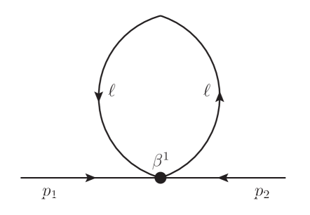
To evaluate the diagram, one must consider the 24 permutations of the momenta entering the vertex. Among these, only 8 conserve the momentum (i.e. ), while the remaining 16 do not.
At the linear level in the calculation can be done explicitly, showing stronger divergences than in the commutative theory [10]. However, the effects of momentum nonconservation cancel out.
Attempting instead a calculation at all orders in , not all diagrams can be explicitly computed [11]. It can be shown, however, that the divergences are suppressed with respect to the noncommutative theory and there are even indications that the integrals might be finite, at least for the interaction (42).
If instead, renormalization is necessary, the phenomenon of UV/IR mixing could still be present, as in other noncommutative models [4]. We recall however that a model that avoids this problem in Moyal theory was proposed by Grosse and Wulkenhaar [26] (GW model). Its main characteristic is that, besides the kinetic and interaction terms, its action also contains a term proportional to . A similar mechanism can be recovered in Snyder theory by considering a curved background (SdS model) [27].
In fact, using the relation (16) between the SdS and Snyder algebra with , and the realization (26) of the Snyder algebra, the action can be reduced, at zeroth order in , , to
| (46) |
The action (46) is identical to that of the free GW model. One may therefore hope that also in this case the IR divergences are suppressed and one can obtain a renormalizable theory.
7 Conclusions
We have reviewed the present status of research on the Snyder model, the earliest example of noncommutative geometry, and the only one that preserves Lorentz invariance. In particular, we concentrated on the definition of a quantum field theory defined in accord with the standard noncommutative formalism, and the issue of renormalizability. It turns out that, although an exact calculation has not been performed in full, there is good evidence of renormalizability and absence of UV/IR mixing, at least in the SdS model.
References
- [1] L.J. Garay, Int. J. Mod. Phys. A 10, 145 (1995); S. Hossenfelder, Liv. Rev. Rel. 16, 2 (2013).
- [2] H.S. Snyder, Phys. Rev. 71, 38 (1947); Phys. Rev. 72, 68 (1947).
- [3] A. Connes, Noncommutative Geometry (Academic Press, 1994); J. Madore, An Introduction to Noncommutative Differential Geometry and its Physical Applications (Cambridge Un. Press, 1999).
- [4] For a review, see e.g. M.R. Douglas and N.A. Nekrasov, Rev. Mod. Phys. 73, 977 (2001); R.J. Szabo, Phys. Rept. 378, 207 (2003).
- [5] S. Majid, Foundations of quantum group theory (Cambridge University Press, 1995).
- [6] G. Amelino-Camelia, Int. J. Mod. Phys. D 11, 35 (2002); Phys. Lett. B 510, 255 (2001).
- [7] J. Kowalski-Glikman, Phys. Lett. B 547, 291 (2002); J. Kowalski-Glikman and S. Nowak, Class. Quantum Grav. 20, 4799 (2003).
- [8] Y.A. Gol’fand, JETP 16, 184 (1963); JETP 17, 842 (1963); JETP 37, 356 (1960); V. G. Kadyshevsky, JETP 14, 1340 (1962); R.M. Mir-Kasimov, JETP 22, 629 (1966); JETP 25, 348 (1967).
- [9] J.C. Breckenridge, T.G. Steele and V. Elias, Class. Quantum Grav. 12, 637 (1995); T. Konopka, Mod. Phys. Lett. A 23, 319 (2008).
- [10] S. Meljanac, S. Mignemi, J. Trampetić and J. You, Phys. Rev. D 96, 045021 (2017); A. Franchino-Viñas and S. Mignemi, Phys. Rev. D 98, 065010 (2018).
- [11] S. Meljanac, S. Mignemi, J. Trampetić and J. You, Phys. Rev. D 97, 055041 (2018).
- [12] M.V. Battisti and S. Meljanac, Phys. Rev. D 79, 067505 (2009); Phys. Rev. D 82, 024028 (2010).
- [13] B. Ivetić and S. Mignemi, Int. J. Mod. Phys. D 27, 1950010 (2018).
- [14] S. Meljanac, D. Meljanac, S. Mignemi and R. Štrajn, Phys. Lett. B 768, 321 (2017).
- [15] C.N. Yang, Phys. Rev. 72, 874 (1947).
- [16] J. Kowalski-Glikman and L. Smolin, Phys. Rev. D 70, 065020 (2004).
- [17] H.G. Guo, C.G. Huang and H.T. Wu, Phys. Lett. B 663, 270 (2008).
- [18] M. Born, Rev. Mod. Phys. 21, 463 (1949).
- [19] S. Mignemi, Class. Quantum Grav. 26, 245020 (2009).
- [20] G. Veneziano, Europhys. Lett. 2, 199 (1986): M. Maggiore, Phys. Lett. B 304, 63 (1993).
- [21] S. Mignemi and R. Štrajn, Phys. Rev. D 90, 044019 (2014).
- [22] S. Mignemi and A. Samsarov, Phys. Lett. A 381, 1655 (2017); S. Mignemi and G. Rosati, Class. Quantum Grav. 35, 145006 (2018).
- [23] G. Gubitosi and F. Mercati, Class. Quantum Grav. 20, 145002 (2013).
- [24] F. Girelli and E. Livine, JHEP 1103, 132 (2011).
- [25] S. Meljanac, Z. Škoda and D. Svrtan, SIGMA 8, 013 (2012).
- [26] H. Grosse and R. Wulkenhaar, Comm. Math. Phys. 256, 305 (2005).
-
[27]
A. Franchino-Viñas and S. Mignemi, in preparation.
Received 02.08.19