High-resolution study of excited states in ¹⁵⁸Gd with (p,t) reactions.

Abstract

The excitation spectra in the deformed nucleus ¹⁵⁸Gd have been studied with high energy resolution by means of the (p,t) reaction using the Q3D spectrograph facility at the Munich Tandem accelerator. The angular distributions of tritons were measured for more than 200 excited states seen in the triton spectra up to 4.3 MeV. A number of 36 excited 0⁺ states (five tentative), have been assigned by comparison of experimental angular distributions with the calculated ones using the CHUCK code. Assignments for levels with higher spins are the following: 95 for 2⁺ states, 64 for 4⁺ states, 14 for 6⁺ states and about 20 for negative parity states. Sequences of states which can be treated as rotational bands are selected. The analysis of the moments of inertia defined for these bands is carried out. This high number of excited states in a deformed nucleus, close to a complete level scheme, constitutes a very good ground to check models of nuclear structure. The large ensembles of states with the same spin-parity offer unique opportunities for statistical analysis. Such an analysis for the 0⁺, 2⁺ and 4⁺ states sequences, for all $K$-values and for well-determined projections $K$ of the angular momentum is performed. The obtained data may indicate on a K symmetry breaking. Experimental data are compared with interacting boson model (IBM) calculations using the $spdf$ version of the model. The energies of the low-lying levels, the transition probabilities in the first bands and the distribution in transfer intensity of the 0⁺ states are calculated and compared with experiment.

I Introduction

The nucleus ¹⁵⁸Gd is located in a region of strong deformation. Excitation spectra of the even-even nuclei in this region are complex. Collective excitations - both of the rotational and vibrational nature - are dominant. The particle-hole nucleon excitations can also contribute to such spectra. Interactions of all these sources of nuclear excitation complicate the understanding of the resulting structures, and therefore a full description has not been achieved yet. In fact, nuclear collective excitations even at low energies still represent a challenge for the theoretical models. At low excitations these states can be analyzed in terms of the beta vibrations, pairing vibrations, spin-quadrupole interaction, shape coexistence, one- and two-phonon states, etc. At higher excitations, one expects multi-phonon states and mixing of all these excitations by the residual interaction. Detailed experimental data on the properties of many excited states of deformed nuclei over an extended excitation energy range are required in order to unravel these aspects.

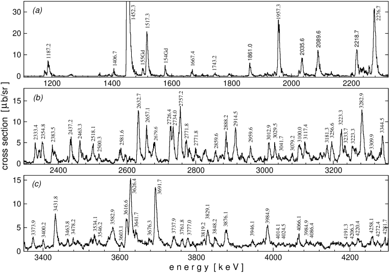
Figure 1: The triton spectrum from the ¹⁶⁰Gd(p,t)¹⁵⁸Gd reaction measured at angle 5^∘. Peak labels represent excitation energies in keV.

Most detailed studies of the collective modes in the nucleus ¹⁵⁸Gd were performed in the radiative capture Gre78 ; Bor99 and in the (n,n${}^{\prime}\gamma$) reaction Gov01 . These studies were very important for a complete determination of the level scheme at low spins and up to low-to-moderate level density, that corresponds to about 2.5 MeV excitation. Nearly 90 levels with low spins of positive and negative parity up to 3 MeV were identified in this region and many of these states were combined into rotational bands. A total of thirteen excited rotational bands with band-head energies below 1.8 MeV were incorporated in the level scheme. They include the octupole-vibrational bands with band-heads 0^- and 1^-, the $\gamma$-vibrational band and three excited $0^{+}$ bands. Several two-quasiparticle bands with band-heads 4⁺, 4^- and 1⁺ were identified too. The study of $\beta^{-}$ decay of ¹⁵⁸Eu Klu74 is most informative among other radioactive decay studies, and has provided 31 excited states and 94 $\gamma$ transitions, all incorporated in a level scheme. The coincidence measurements have provided reliable branching ratios for members of the $\gamma$-vibrational band and members of $K^{\pi}=0^{-}$ and 1^- octupole bands. Precise excitation energies, reduced transition probabilities and decay branching ratios of numerous $I=1$ states were extracted from the energies and angular distributions of the scattered photons in the nuclear resonance fluorescence experiment Pit89 . The ground 0⁺ band and octupole 1^- band were extended to the 12⁺ and 9^- states, respectively, by Coulomb excitation Sug93 . However, all these studies had many difficulties at states above $\sim$2 MeV of excitation energy, and completeness of data was rapidly lost.

The most productive mode of obtaining information about collective and other excitation modes is the use of the direct reaction of two-neutron transfer, which, for practical reasons, is mainly the (p,t) reaction. It was found to be a very effective tool to study the multiple 0⁺ excitations in actinide and rare earth nuclei Ack94 ; Bal96 ; Lev94 ; Lesh02 ; Wir04 ; Lev09 ; Lev13 ; Lev15 ; Spi13 ; Mey06 ; Buc06 ; Bet09 ; Ili10 . For some nuclei in these studies, extensive information was also obtained for states with higher spins of the positive and negative parity up to 6 Buc06 ; Lev09 ; Lev13 ; Lev15 ; Spi18 . So far, almost all the studies with the (p,t) reaction were performed for excitation energy below 3 MeV. The study of 0⁺ states up to about 4.2 MeV for ¹⁵⁸Gd was recently performed in Ref. Lev19 , and of 0⁺ and 2⁺ states in the case of ¹⁶⁸Er (see Ref. Buc06 ).

Several theoretical approaches were aimed to explain the results obtained by these studies, e.g., the interacting boson model (IBM) Iach87 ; Casten01 and its expansion using the $s,p,d,f$ bosons Zam01 ; Zam03 , the projected shell model (PSM) Har95 ; Sun03 , the quasiparticle-phonon model (QPM) Sol89 ; QPM ; Lo04 ; Lo05 , and a model including the monopole pairing, the quadrupole-quadrupole and spin-quadrupole forces in the framework of the random phase approximation (RPA) Mur10 . Both QPM and IBM predict a number of 0⁺ states and a cumulative cross section for their excitation which basically agreed with experiment for low energies. However, both models fail to give a detailed explanation of the individual states. Most excitations calculated in the IBM have two $pf$ bosons in their structure, therefore being related to the presence of a double octupole structure. At the same time the QPM predicts only minor double-octupole phonon components in states below 3 MeV.

This paper presents results of new measurements, with the ¹⁶⁰Gd(p,t)¹⁵⁸Gd reaction, of positive and negative parity states in the region from 1.7 MeV up to 4.3 MeV excitation. We identified in ¹⁵⁸Gd 230 states with different spins in this energy interval. The angular distributions of tritons were measured for 205 states seen in the triton spectra. Firm assignments of spins and parities have been obtained for most of these excited states by comparison of experimental angular distributions with the calculated ones using the distorted wave Born approximation (DWBA). Sequences of states were selected that can be treated as rotational bands. They are used for statistical analysis of sequences of 2⁺ and 4⁺states with different fixed $K$ projection of the angular momentum on the symmetry axes. A new approach is used for fitting the nearest neighbor-spacing distributions (NNSD) to investigate the fluctuation properties of the experimental spectra. The nature of 0⁺ and other states is analysed in the frame of the IBM.

II Experiment, analysis and results

II.1 Experimental details

The experiments have been performed at the Tandem accelerator of the Maier-Leibnitz-Laboratory of the Ludwig-Maximilians-University and Technical University of Munich using a 22 MeV proton beam. The reaction products were analyzed with the high-precision Q3D spectrograph. A long (1.4 m) focal-plane detector provides the $\Delta E$/$E$ particle identification of the light ejectiles and position determination Wir01 . The different runs were normalized to the beam current integrated into a Faraday cup placed behind the target.

The experiment in the high-energy region 3.0 - 4.3 MeV has been performed on a 110 $\mu$g/cm² target of isotopically enriched ¹⁶⁰Gd (98.10%) with a 14 $\mu$g/cm² carbon backing. Known impurities in the target material consist of ¹⁵⁸Gd (0.99%), ¹⁵⁶Gd (0.33%), and ¹⁵⁷Gd (0.44%). The resulting triton spectra have a resolution of 4 - 7 keV (FWHM) and are background-free. The acceptance of the spectrograph $\Delta\Omega$ was 14.43 msr for all angles, except for the most forward angle 5^∘, where it was 7.50 msr. Typical beam current was around 1.0 $\mu$A. The angular distributions of the cross sections were obtained from the triton spectra at eight laboratory angles from 5^∘ to 40^∘ in step of 5^∘. The low energy spectra in the interval from 0 to 3.4 MeV have been also measured at the angle of 5^∘ for three magnetic setting, which are all overlapping with the neighboring regions. For the calibration of the energy scale, the triton spectra from the reaction ¹⁵⁴Gd(p,t)¹⁵²Gd have been measured at the same magnetic setting. In this way, the high energy spectrum of ¹⁵⁸Gd was calibrated by the known energies of the nucleus ¹⁵²Gd.

The experiment in the low-energy region 1.7 - 3.2 MeV was performed with a 125 $\mu$g/cm² target of ¹⁶⁰Gd. The acceptance $\Delta\Omega$ was 9.8 msr for 6^∘ and 14.5 msr for other angles. The resulting triton spectra have a slightly lower resolution of 8 - 9 keV (FWHM). For the calibration of the energy scale, the triton spectra from the reaction ¹⁷²Yb(p,t)¹⁷⁰Yb were measured at the same magnetic settings. The low-energy spectrum calibrated in such a way has a 250 keV overlap with the high-energy spectrum fixed by the previous experiment. Many levels of ¹⁵⁸Gd well-known from the resonance capture and from the (n,n${}^{\prime}\gamma$) reaction are correctly fitted with this calibration in the low energy region. The spectra in low and high energy intervals calibrated by the corresponding reactions ¹⁵⁴Gd(p,t)¹⁵²Gd and ¹⁷²Yb(p,t)¹⁷⁰Yb coincide in the overlapping region. The difference in the energies determined by these calibrations in the overlapping region does not exceed 1 keV.

The details of the experiment and especially those of the energy calibration procedure are given in Ref. Lev19 which deals with the study of excited 0⁺ states in ¹⁵⁸Gd. Some results of the (p,t) experiment at low energies performed by a Yale-Munich-Köln-Bucharest collaboration (the YMKB experiment) Mey06 were also analysed in this publication.

Fig. 1(a-c) shows the triton spectrum over the energy interval from 1.0 to 4.3 MeV, taken at the detection angle of 5^∘. Some strong peaks are labeled by their energies in keV.

The analysis of triton spectra was performed by using the program GASPAN Rie91 . Peaks of the spectra which are measured at 5^∘ degree have been identified for 230 levels, though the angular distributions for all eight angles could be measured only for 205 levels. The differential cross sections were calculated by the following equation

$$\frac{d\sigma(\theta)}{d\Omega}=\frac{N(\theta)}{\Delta\Omega\times I_{total}\times D_{target}/\cos(\theta)}$$ (1)

Here $N(\theta)$ is the number of tritons measured for each state at a Q3D angle $\theta$, corrected for the dead time of the data-acquisition system, $\Delta\Omega$ is the acceptance of the spectrograph, $I_{total}$ is the total number of protons measured by the Faraday cup, and $D_{target}$/cos($\theta$) is the effective target thickness. The angle $\theta$ is also the angle between the target area and the beam axis. To determine the integrated (p,t) excitation cross section, the differential cross sections were integrated over the covered angular range.

II.2 DWBA analysis

To determine the value of the transferred angular momentum $L$ and spin ($I=L$) for each level in the final nucleus ¹⁵⁸Gd, the observed angular distributions are compared with calculations using the DWBA. The coupled-channel approximation (CHUCK3 code of Kunz Kun ) and the optical potential parameters suggested by Becchetti and Greenlees Bec69 for protons and by Flynn et al. Fly69 for tritons have been used in the calculations.

In principle, the transfer of the two neutrons coupled to spin 0 should contain the contribution of different $j$ spins of the two particles. The orbitals close to the Fermi surface have been used as the transfer configurations. For ¹⁵⁸Gd and ¹⁶⁰Gd, such configurations include the orbitals which correspond to those in the spherical potential, namely, $2f_{5/2}$, $1h_{9/2}$, $1h_{11/2}$, and $1i_{13/2}$. Since we do not know the dominant transfer for each state, all of them were tested to get a better fit of the experimental angular distributions. The angular distributions for the 0⁺ states are reproduced very well by a one-step process. Only two configurations in possible combinations have been taken into account, that simplifies the calculations. The experimental results and the details of the DWBA calculations for 0⁺ states are presented in the publication Lev19 . Thirty-two new excited 0⁺ states (four tentative) have been assigned up to the 4.3 MeV excitation energy. Thus, the total number of 0⁺ excited states, besides the ground state (g.s.) in ¹⁵⁸Gd, was increased up to 36, the highest number of such states observed so far in a single nucleus.

In the present detailed analysis, an additional weak 0⁺ excitation at 3365.9 keV was identified. The angular distribution for this state is shown in Fig. 2. Another problem met in the previous study Lev19 is a tentative 0⁺ assignation for two states at 3344.5 and 3819.2 keV. For these states the reason of this tentative assignment is the absence of a deep minimum at an angle of about 17^∘ (Fig. 2). The calculated angular distribution has such a form at the transfer of a pair of $i_{13/2}$ neutrons but only for a lower excitation energy. It proved impossible to fit well the experimental angular distributions by using the actual reaction energies in such calculations. Calculations for transferring other angular momenta do not allow to describe the experimental angular distributions, and thus, rule out other spin assignments. There is another possible explanation for this shape of the angular distribution: the overlap with another level having a very close energy. The overlap of the angular distributions for the 0⁺ state with those for a 4⁺ state explains the experimental angular distributions for both levels as demonstrated in Fig. 2. Of course, this is only a tentative explanation.

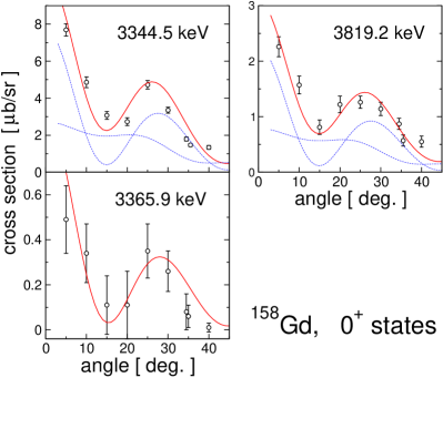
Figure 2: The 0⁺ state at 3365.9 keV additionally identified in this study and suggested fits for the states 3344.5 and 3819.2 keV. The blue lines represent the result of calculations for the 0⁺ and 4⁺ states, respectively, the sum of which fits the experimental angular distributions.

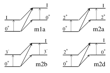
Figure 3: Schemes of the CHUCK3 multi-step calculations tested with spin assignments of excited states in ¹⁵⁸Gd (see Table LABEL:Tab:expEI).

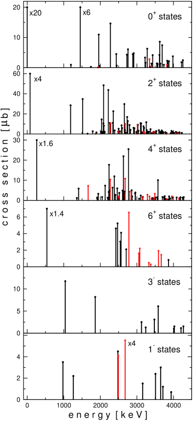
Figure 4: The (p,t) strength integrated in the angle region 0^∘ - 45^∘ for 0⁺, 2⁺, 4⁺, 6⁺, 3^- and 1^- states in ¹⁵⁸Gd. The levels identified reliably and tentatively are indicated by black filled circles and by red open diamonds, respectively.

The situation is more complex for the states with higher spins. Only a few experimental angular distributions could be fitted by the calculated ones for the one-way direct transfer of two neutrons with nonzero orbital angular momentum. The angular distribution for such states may be altered due to inelastic scattering (coupled channel effect), treated here as multi-step processes. Taking into account these circumstances, one can obtain spin assignments for most excited states in the final nucleus ¹⁵⁸Gd by fitting the angular distributions obtained in the DWBA calculations to the experimental ones. The multi-step transfer schemes used in the present DWBA calculations are displayed in Fig. 3. The best fit is  achieved by changing the amplitudes of each branch in  the multi-step transfer. The shape of the angular distribution in this case may be drastically different from the shape of that for the one-way transfer. Moreover, with the projectile energy used in the experiment, the shape of the one-step angular distribution also changes with increasing of the excitation energy (see below). Nevertheless, the selectivity of such spin assignments is quite reliable. The spins assigned in such a way are confirmed by comparison with the spin values well-defined in other experiments.

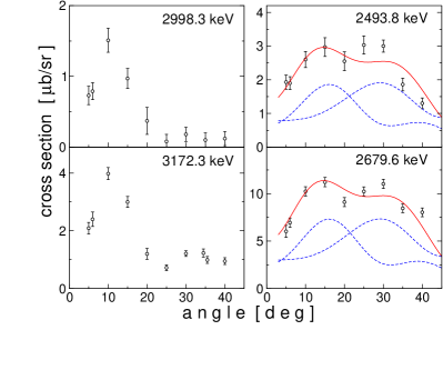
Figure 5: Angular distributions for the states with problematical fits. See text for details.

The results of this study concerning all the states identified in the (p,t) reaction are collected in Table LABEL:Tab:expEI. They are also presented in a compressed form in Fig. 4. For the states below 1743.2 keV we obtained only the absolute cross sections at 5^∘ because the angular distributions themselves were not measured. Therefore, their spins were not assigned in this work and are not shown in Table LABEL:Tab:expEI. Excitations of the 0⁺ and 2⁺ states in the nuclei of the impurity isotopes in the target material manifest themselves in the observed triton spectrum. The 1577 keV excitation is important in our study. The 0⁺ assignment at 1576.932(16) keV from the (n,$\gamma$) reaction Gre96 was confirmed in the (p,t) reaction Lesh02 . However, later, no $\gamma$-rays were detected as decaying the level 1577 keV when studying the 0⁺ states in the (n,n${}^{\prime}\gamma$) reaction Lesh07 . The triton energy associated with this level is near that for the g.s. in the ¹⁵⁶Gd(p,t)¹⁵⁴Gd reaction. Therefore, the corresponding peak can be interpreted as an excitation on the ¹⁵⁶Gd contamination in the target material. The observed cross section 5.6 $\mu$b/sr is somewhat smaller than the calculated 7.8 $\mu$b/sr when using the cross section for the ¹⁵⁶Gd(p,t)¹⁵⁴Gd reaction from Ref. Mey06 . Thus, the present (p,t) data do not confirm presence of the 1577 keV level in the nucleus ¹⁵⁸Gd.

Spins and parities for ten states above 1743 keV are not shown in Table LABEL:Tab:expEI. The energies of these states were determined in the spectrum at 5^∘ measured with good statistical accuracy. However, identification of the corresponding peaks in the spectra for other angles was difficult and consequently their angular distributions could not be measured. The shape of the angular distributions for two states, 2998.3 and 3172.3 keV, could not be attributed to any calculated angular distribution (Fig. 5). However, since the beginning of the angular distributions is close to that for the 2⁺ and 1^- states, these spins were assigned tentatively for these states. Finally, the angular distributions for two states at 2493.8 and 2679.6 keV can be fitted by calculated ones for one-way transfer to a 1^- state. However, their cross sections are excessively high as compared with other 1^- states observed in ¹⁵⁸Gd. Therefore, an alternative description of the angular distribution can be considered. Namely, the superposition of two distributions, for 2⁺ and 4⁺ states, as shown in Fig. 5. That is, the corresponding peaks in the triton spectrum are assumed to be doublets. Both options are included in Table LABEL:Tab:expEI as tentative assignments.

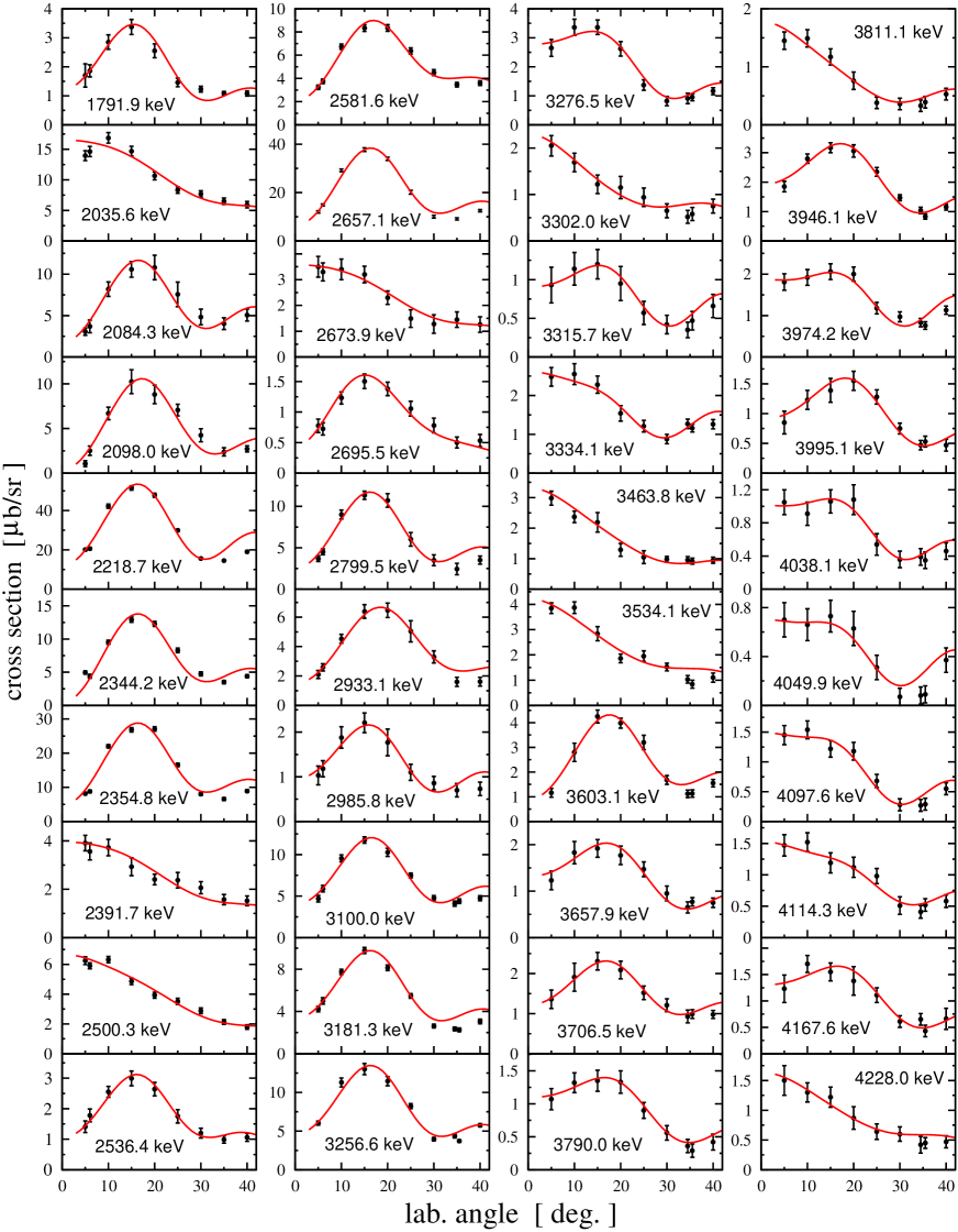
Figure 6: Angular distributions of assigned $2^{+}$ states in ¹⁵⁸Gd and their fit with CHUCK3 calculations. The $(ij)$ transfer configurations and schemes used in the calculations for the best fit are given in Table LABEL:Tab:expEI.

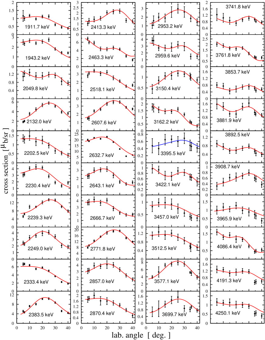
Figure 7: Angular distributions of assigned $4^{+}$ states in ¹⁵⁸Gd and their fit with CHUCK3 calculations. The $(ij)$ transfer configurations and schemes used in the calculations for the best fit are given in Table LABEL:Tab:expEI. The red lines indicate firm assignments and the blue lines are putative ones.

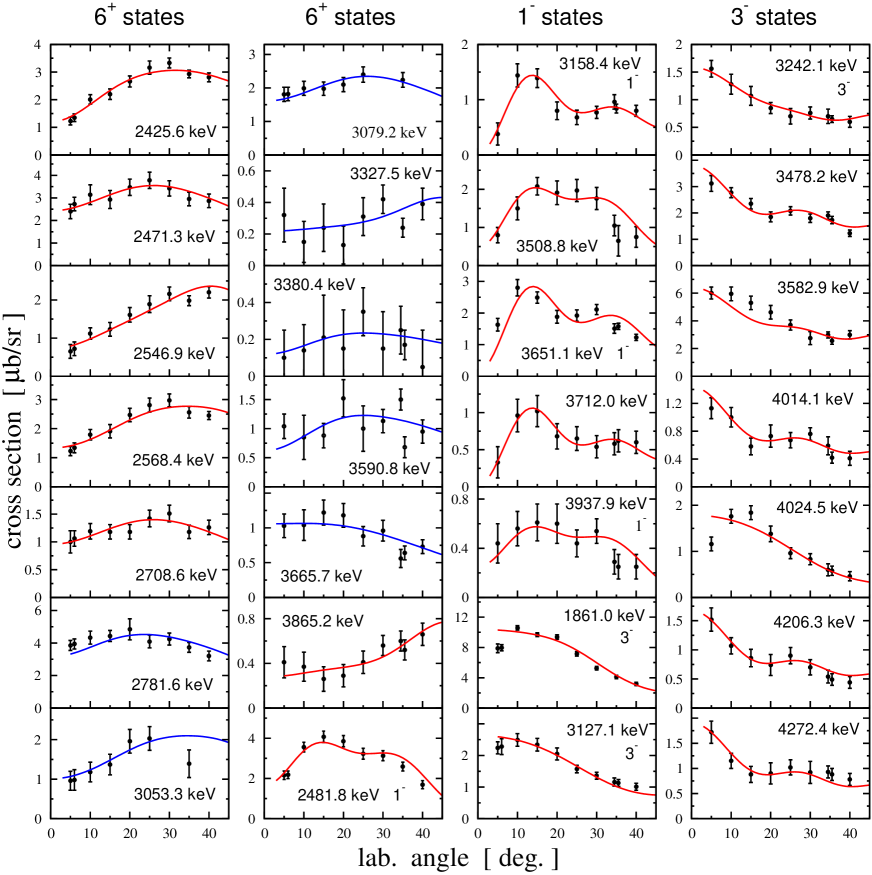
Figure 8: Angular distributions of assigned $6^{+}$, $1^{-}$ and $3^{-}$ states in ¹⁵⁸Gd and their fit with CHUCK3 calculations. The $(ij)$ transfer configurations and schemes used in the calculations for the best fit are given in Table LABEL:Tab:expEI. The red lines indicate firm assignments and the blue lines are putative ones. The red dashed lines are calculations with changed potential parameters for tritons (see text).

The ground state rotational-band members are excited up to $8^{+}$ in such experiments Lev09 ; Lev13 ; Lev15 ; Spi13 ; Spi18 (for ¹⁵⁸Gd the 8⁺ state peak is overlapped by the peak of the excitation of the g.s. ¹⁵⁶Gd impurity). Nevertheless, angular distributions could be measured up to $6^{+}$. As one can see from Fig. 4, the cross section is steadily decreasing with increasing spin. Figs. 6, 7 and 8 show the experimental data for the angular distributions for 2⁺, 4⁺, 6⁺, as well as for 1^-, 3^- states, all given in $\mu$b/sr and their values are plotted with symbols with error bars while the Q-corrected CHUCK3 calculations are shown by full lines. The solid (red) lines present the firm assignments and the solid (blue) lines show tentative assignments. Fitting of the calculated angular distributions to the experimental ones allowed to determine the spins and parities for most of final states which were identified.

II.3 Some specific features of angular distributions in the extended energy range.

0⁺ states. Excitations of 0⁺ states are possible only in the one-way transfer of a pair of neutrons. The shape of angular distribution depends only slightly on the neutron configuration and is characterized by a steeply rising cross section at small angles, a sharp minimum at angles of 10^∘-17^∘ and a weak maximum at angles of 25^∘-35^∘. A significant shape deviation for ¹⁵⁸Gd was observed only for two excitation energies and is tentatively explained by a possible overlap with the angular distribution of another state (see above).

2⁺ states. The angular distribution for the 2⁺ states calculated for the one-way transfer of a pair of neutrons has a ”bell-shaped” form with a deep minimum at small angles and a maximum at angles of 15^∘-18^∘. As an example one can see the distribution for the energy of 2218.7 keV in Fig. 6. The experimental angular distributions have such a form for many excitation energies. However, the detailed fitting needs in some cases at least small inclusions of two-step processes involving inelastic scattering through intermediate states. The calculated and experimental angular distributions also change the shape with increasing excitation energy, even for the one-way transfer. The cross section at small angles gradually increases with increasing excitation energy up to the maximum values at angles of 15^∘-18^∘. This can be seen, for example, already for the energy of 3315.7 keV in Fig. 6. A special case is represented by excitations in which inelastic scattering through intermediate states in the two-step processes plays a significant or even dominant role. As an example, such a case is the excitation of the 2⁺ state in the ground state band. In this case, the angular distribution has a strong maximum at small angles, but, unlike the case of the 0⁺ states, there is not a deep minimum. The 2⁺ assignments in cases of such angular distributions are confirmed by known spins in previous studies Lev09 ; Lev13 ; Lev15 for the states 2500.3 and 2673.9 keV in this work (see Fig. 6).

4⁺ states. The angular distributions for the 4⁺ states are reproduced with small admixture of two-step processes involving inelastic scattering of intermediate states only for some excitation energies, as for example for the state at 2049.8 keV in Fig. 7. With increasing excitation energy, the calculated and experimental angular distributions even at the one-way transfer change the shape similar to 2⁺ states. The cross section at small angles gradually decreases and there is an increasing maximum at an angle of about 30^∘. It is seen in Fig. 7 for instance for the excitation energy of 2132.0 keV. Similarly to the 2⁺ states, a special case is represented by the excitation in which the multi-step processes play a significant role. In this case, the angular distribution has a maximum at small angles, although it is not as pronounced as that for 2⁺ states, while the deep minimum of the 0⁺ states is absent. It is seen, e.g., in Fig. 7, for the excitation energy 2202.5 keV.

6⁺ states. The calculated angular distributions for 6⁺ states with small admixture of two-step processes have a pronounced maximum at the angle of about 45^∘ at transfer of the f_5/2, h_9/2 and h_11/2 neutron pairs (the energy of 2546.9 keV in Fig. 8 as an example), and almost flat shape at transfer of i_13/2 neutron pair (energy of 3327.5 keV in Fig. 8 as another example). Taking into account two-step processes leads to a shift of the maximum to smaller angles.

1^- states. The angular distributions for the 1^- states are reproduced by the calculated ones for the one-step transfer. They have two pronounced maxima and, therefore the assignment is reliable despite rather small cross sections of their excitation (Fig. 8).

3^- states. The angular distributions for the 3^- states are reproduced by the calculated ones for the one-step transfer for most excitation energies (the energy of 3478.2 keV in Fig. 8 as an example). Only some of them need a small inclusion of the two-step processes. The maximum of such a distribution is found at the angle of 0^∘ with the exception of two energies of 1861.0, 3127.1 and 4024.5 keV. The maximum of the angular distribution for these energies occurs at an angle of about 15^∘, and is not fitted by calculations with the potential parameters used for all other states. The spin 3^- of the first such state is well known from previous studies Nic17 . Therefore, this spin is assigned also for other two states. Minor changes of the parameters for tritons helped to fit these angular distributions, namely the use of the triton potential parameters suggested by Becchetti and Greenlees Bec71 .

Table 1: Energies of levels in ¹⁵⁸Gd, spin assignments from the CHUCK3 analysis, the (p,t) reaction cross sections at 5^∘, as well as integrated cross section over the measured values (i.e. 5^∘ to 40^∘), and the reference to the schemes used in the DWBA calculations.

ENSDF Ref. Nic17		Present data				Way of
Energy [keV]	$I^{\pi}$	Energy [keV]	$I^{\pi}$	d$\sigma$/d$\Omega$	$\sigma_{\mbox{integ.}}$[$\mu$b]	fitting
				at 5∘ [$\mu$b/sr]
0.00	0+	0.13		1435 12
79.514	2+	79.3 3		267 4
261.458	4+	260.1 3		51.2 2
539.022	6+	538.8 5		1.9 3
156Gd	g.s.	904.2 3		11.7 7
977.156 2	1-	977.3 4		2.0 4
156Gd	2+	992.9 12		2.1 4
1023.698 3	2-	1023.4 12		0.2 2
1041.640 3	3-	1041.6 3		12.8 7
1176.481 5	5-	1176.7 5		3.5 4
1187.148 3	2+	1187.4 4		11.4 7
1196.164 7	0+	1196.1 8		3.3 4
1259.870 2	2+	1260.8 8		0.6 3
1263.515 3	1-	1262.7 6		1.1 3
1358.472 3	4+	1358.4 4		1.3 3
1380.634 6	4+	1379.7 12		0.4 3
1406.702 3	4+	1406.4 3		4.0 5
1452.353 6	0+	1452.3 6		423 6
155Gd	g.s.	1503.3 3		6.2 6
1517.480 3	2+	1517.3 10		37.9 14
155Gd	5/2-	1563.5 20		0.4 3
154Gd	g.s.	1577.0 4		5.6 6
1576.932 16	0+
1653	2+	1650.0 24		0.4 3
1667.373 6	(4+)	1667.3 4		4.0 5
154Gd	2+	1701.4 12		1.0 3
1716.807 5	5-	1717.9 15		0.7 3
1743.147 14	0+	1743.2 2	0+	1.9 2	0.8 2	sw.h09
1791.797 9	2+	1791.9 5	2+	1.9 4	2.9 3	sw.ii
1861.281 7	3-	1861.0 4	3-	8.9 7	10.0 4	m2a.h09
		1868.1 8	(2+)	0.6 4	0.9 4	m1a.h09
1894.578 21	(2+)	1894.4 8	2+	0.9 3	1.7 4	m1a.h09
		1911.7 8	4+	1.3 4	1.3 4	m1a.ii
1920.264 6	4+	1920.9 6	4+	2.0 4	1.6 2	m1a.h11
1935.5 6	0+	1936.5 15	(0+)	1.0 2	0.3 1	sw.h09i
		1943.2 8	4+	2.7 5	3.6 3	m1a.ii
1952.425 25	(0+)	1952.2 1		0.4 5
1957.27 9	0+	1957.3 3	0+	39.0 10	11.0 8	sw.fi
1964.12 2	2+
1972.2 31	(0+)	1977.6 12	0+	1.3 2	0.6 2	sw.h11i
		2026.3 8	2+	3.5 5	2.3 4	m1a.h11
2035.70 3	2+	2035.6 5	2+	15.2 9	14.5 10	m1a.ii
		2049.8 10	4+	1.2 3	1.7 3	m2a.h11
		2056.5 8	2+	1.2 4	2.2 4	sw.h09
2083.639 24	2+	2084.3 6	2+	3.3 5	10.6 16	sw.h09
2089.254 8	2+	2089.6 5	2+	15.3 8	52.7 24	m1a.h09
2095.20 16	(4+)
		2098.0 1	2+	1.1 3	8.3 12	sw.h09
		2113.5 6	2+	1.0 2	2.5 5	sw.h09
2120.25 4		2120.8 8	2+	1.0 2	2.1 3	m1a.h09
2134 7		2132.0 6	4+	2.0 2	7.3 5	m1a.h11
2153.178 9	(2,3)+	2153.4 10	3+	0.6 1	3.0 4	m2a.h09
		2202.5 5	4+	1.5 2	1.4 3	m1a.h11
		2218.7 5	2+	21.8 6	47.6 10	sw.h09
		2230.4 6	4+	3.6 3	4.2 4	m1a.ii
		2239.3 5	4+	5.7 4	17.7 10	m1a.h11
2249.61 5	2+,3,4+	2249.0 6	4+	2.7 3	5.3 5	m1a.h11
2260.162 18	1,2+	2260.3 5	2+	5.2 3	11.9 7	sw.h09
2269.269 14	(0,1,2)+	2271.8 10	(4+)	8.3 3	11.3 16	m1a.h11
2276.76 5	0+	2276.7 4	0+	52.3 15	14.6 9	sw.h09
2283.2 6		2283.4 10	(2+)	10.2 12	11.5 8	sw.ih
		2333.4 5	4+	7.2 4	6.9 3	m1a.ii
2340.3 3	2+
2344.7 5	2+,3+	2344.2 5	2+	5.4 3	12.1 5	m1a.h09
2355.0 5	1+,2+	2354.8 4	2+	9.1 4	22.6 8	m1a.h09
2384		2383.5 4	4+	5.5 3	13.0 6	m1a.h11
		2391.7 5	2+	4.3 3	3.6 4	m1a.ii
		2413.3 8	4+	1.1 2	2.7 3	m1a.h11
		2425.6 8	6+	1.3 2	5.0 3	m2b.i13
		2437.2 4	0+	11.9 4	4.5 3	sw.h09
2446.49 15	1	2445.9 8	0+	1.5 2	0.7 3	sw.h09
		2463.3 5	4+	7.4 4	6.5 6	m1a.ii
		2471.3 6	6+	2.6 3	5.7 6	m2a.h09
2480.5 14		2481.8 6	1-	2.4 2	4.8 5	sw.hi
		2493.8 10	(1-)	1.4 2	4.1 4	sw.h09i
		or	($2^{+}$+4+)			m1a.h09
2499.22 10	(1,2)+	2500.3 4	2+	6.8 4	5.7 3	m1a.h11
		2507.8 10		1.6 3
		2518.1 6	4+	2.9 2	3.7 3	m1a.i13
2538.7 7	(2+)	2536.4 8	2+	1.5 2	2.9 3	m1a.h09
		2546.9 10	6+	0.7 2	3.3 3	m2b.h09
		2568.4 6	6+	1.3 2	4.5 4	m2a.h09
		2578.4 8		3.1 8
		2581.6 10	2+	3.5 8	9.4 4	m1a.h09
2594.73 20	(+)	2594.9 5	2+	2.9 3	6.4 4	m1a.h09
		2607.6 10	4+	1.6 2	4.9 3	m1a.h11
		2615.9 6		1.6 2
2630.9 5	(+)	2632.7 4	4+	21.7 9	22.0 7	m1a.i13h11
2644.3 7		2643.1 5	4+	2.5 3	3.4 4	m1a.h11i13
2656.9 5		2657.1 3	2+	13.0 5	32.4 10	m1a.h09
		2666.7 10	4+	4.0 4	4.7 5	m1a.h11
2674.56 18	(1),2+	2673.9 10	2+	4.3 6	4.1 6	m1a.ii
		2679.6 8	(1-)	6.5 7	22.2 9	sw.h09i
		or	(2++4+)			m1a.h09
		2695.5 10	2+	0.8 1	1.6 2	sw.h09
		2708.6 10	6+	1.0 1	2.3 2	m2a.h09
		2726.4 4	0+	12.4 6	4.3 7	sw.fi
		2734.0 4	2+	10.8 5	18.4 10	m1a.h09
2750.43 19		2750.3 4	2+	8.4 9	14.0 18	m1a.h09
2758.7 5	(+)	2757.2 4	0+	15.8 10	6.1 9	sw.h09i
2761.96 21		2762.5 9		1.1 4
2769 7		2771.8 4	4+	7.5 4	25.5 11	m1a.h11
2782.4 5	(+)	2781.6 6	(6+)	4.2 3	7.1 7	m2a.h09
		2799.5 4	2+	4.0 3	9.8 11	m1a.h09
		2808.4 6	(4+)	1.6 3	4.7 10	m2a.h11
2822.7 5	1-	2822.6 6		2.6 4	2.1 8
2829.6 7	(+)	2828.5 5	2+	3.7 4	4.6 5	m1a.ii
		2857.0 5	4+	3.4 3	5.5 6	m1a.ii
		2870.4 10	4+	1.8 3	2.2 3	m1a.ii
2878.8 4	2+,3	2877.2 10		2.0 3
2886		2888.2 4	0+	9.3 5	4.5 4	sw.h11i
2909.6 5		2909.4 8	2+	3.0 5	6.7 12	m1a.h09
2913.4 7		2914.5 5	0+	10.9 6	4.8 9	sw.h09i
2934.6 11		2933.1 8	2+	2.3 3	6.3 7	m1a.h09
		2953.2 10	4+	1.2 3	3.8 9	m1a.h11
2961.7		2959.6 8	4+	4.3 4	4.3 8	m2a.h11
2964.3 5	2+	2965.8 20		0.5 3
2985.9 5	1(+)	2985.8 7	2+	1.1 2	1.8 3	m1a.h09
		2998.3.2 9	(1-,2+)	0.8 2	0.5 2
3011.9 5	2+,3+	3012.9 6	2+	6.6 4	9.9 6	m1a.h09
3029.2 6		3029.5 4	2+	5.6 4	10.0 6	m1a.h09
		3041.7 8	(2+)	1.7 3	3.4 2	m1a.h09
		3053.3 10	(6+)	1.1 2	1.8 3	m2a.h09
3060.0 4	2+,3	3061.5 8	4+	1.3 2	0.9 2	m1a.h11i
3080.0 6		3079.2 6	(6+)	2.3 3	2.4 2	m2a.h09
		3100.0 4	2+	5.1 4	10.7 6	m1a.h09
		3105.6 6	4+	2.9 4	2.7 3	m1a.h11
3118.5 15		3117.4 3	2+	6.0 3	11.5 5	m1a.h09
		3127.1 4	3-	2.4 3	2.5 2	m2a.h09
3141.5 7		3143.5 6	2+	0.9 11	1.7 3	m1a.h09
		3145.2 16		1.7 11
3150.8 7	(+)	3150.4 20	4+	0.1 2	1.7 2	m1a.h11
3160.8 7	1-	3158.4 10	1-	0.4 2	1.6 2	sw.ii
		3162.2 5	4+	1.9 3	1.9 3	m1a.i13
3171.1 7		3172.3 4	(1-,2+)	2.3 2	2.6 3
		3181.3 4	2+	4.6 3	8.3 4	m1a.h09
3195.4 6		3195.9 3	2+	4.6 6	6.6 6	m1a.h09
3200.8 6	2+,3	3200.2 18	(2+)	2.0 6	0.6 4	m2a.ih09
		3215.9 15	(2+)	1.2 4	1.3 2	m1a.h09
		3223.3 3	0+	10.9 5	3.3 3	sw.h09i
3234.5 5		3233.7 4	0+	5.2 3	1.6 2	sw.h09i
		3242.1 6	3-	1.7 3	1.4 2	sw.h09
		3256.6 4	2+	6.6 3	12.8 6	m1a.h09
3263.8 7		3265.6 8	2+	3.9 2	4.3 3	m1a.h09
		3276.5 7	2+	2.7 3	2.7 3	m2a.h09i
		3282.9 8	0+	19.5 5	6.3 4	sw.fi
3287.9 5		3288.1 7	(4+)	4.3 10	3.1 5	sw.ii
		3302.0 6	2+	2.2 2	1.6 3	m1a.ii
		3309.9 5	2+	2.7 4	2.1 3	m1a.ii
		3315.7 14	2+	1.0 4	1.2 3	sw.h09i
		3327.5 10	(6+)	0.3 2	0.5 2	sw.h09
		3334.1 5	2+	2.7 3	2.5 3	sw.h09i
		3344.5 4	(0+	8.4 4	4.8 5	sw.ih09
			+4+)		2.0 5	m1a.h11
		3365.9 15	0+	0.5 2	0.3 2	sw.h09i
		3373.4 9	2+	4.0 3	5.2 4	m1a.h09
		3380.4 15	(6+)	0.1 1	0.3 3	m2b.ii
		3388.6 10	(0+)	1.1 2	0.3 2	sw.h09i
		3395.5 4	(4+)	0.5 3	1.0 3	sw.ii
		3400.2 9	0+	2.7 3	1.3 3	sw.h11i
3411.7 5		3412.1 11	2+	0.9 2	0.9 2	sw.h09i
		3422.1 10	4+	1.1 2	1.3 2	sw.hi
		3431.8 8	0+	11.2 4	4.2 3	sw.h09i
3436.4 5	(+)	3438.8 9	(2+)	2.3 3	2.0 3	m1a.ii
3448.8 5	(+)	3447.8 9	2+	2.1 2	1.9 2	sw.ii
		3457.0 12	4+	1.1 2	1.1 3	m1a.ii
		3463.8 9	2+	3.2 3	2.2 3	m2a.ih
3469.8 7		3472.2 18	(4+)	0.9 3	1.1 3	sw.h09i
		3478.2 10	3-	3.1 3	3.4 3	sw.ih
		3484.7 22	(4+)	1.0 3	1.1 3	sw.ii
		3490.4 11	(4+)	2.7 4	3.6 3	sw.ii
		3496.8 11	(2+)	1.4 2	2.2 2	m1a.h09+0.8
		3508.8 9	1-	0.8 2	2.6 5	sw.h11
		3512.5 9	4+	1.2 2	1.5 3	m1a.ii
		3524.4 7	2+	3.0 2	3.0 3	m1a.ii
3534.8 6	(+)	3534.1 6	2+	4.0 2	3.1 3	m1a.ii
		3546.2 7	0+	2.2 2	1.4 3	sw.h11i
		3558.5 12	4+	0.8 2	1.7 3	sw.ii
3570.7 6		3569.6 7	0+	3.0 3	1.2 2	sw.h09i
3576.8 7	1	3577.1 9	4+	4.3 5	10.9 10	m1a.h11
		3582.9 7	3-	6.2 5	6.6 7	sw.h09
		3590.8 10	(6+)	1.6 2	2.1 5	m2a.ih09
		3603.1 10	2+	1.2 2	3.8 3	m1a.h09
		3616.6 8	0+	10.8 4	4.2 3	sw.h09i
3626.9 6	(+)	3626.4 8	0+	24.6 5	8.6 4	sw.fi
		3635.6 4	2+	2.3 3	2.2 3	m1a.ii
		3641.7 8	0+	4.4 4	1.3 3	sw.h09i
		3651.1 9	1-	1.9 2	3.2 3	sw.ih
3655.4 8	1,2+	3657.9 4	2+	1.2 2	2.1 3	m1a.hi
3663.3 10		3665.7 10	(6+)	1.2 2	1.6 3	m1a.ii
		3676.3 9	2+	2.6 3	2.5 4	m1a.ii
		3681.3 13	2+	1.1 3	3.8 4	m1a.hi
		3691.7 8	0+	22.2 6	7.4 5	sw.fi
		3699.7 14	4+	1.3 3	1.8 4	m1a.h11
		3706.5 10	2+	1.9 3	2.5 3	m1a.h09
		3712.0 4	1-	0.4 2	1.2 3	sw.ii
		3721.2 11	2+	1.1 2	1.5 3	m1a.h09
		3737.9 11	0+	2.9 7	0.9 2	sw.h09i
		3741.8 15	4+	1.7 7	1.6 3	sw.h09i
		3761.8 6	4+	2.5 2	2.3 2	m1a.ii
		3777.0 6	2+	2.9 2	1.9 2	m1a.ii
		3784.5 4	4+	0.2 2	0.8 2	sw.h09
3794.6 10		3790.0 9	2+	1.2 2	1.4 2	m1a.h09
		3802.5 10	(2+)	1.0 2	0.3 2	m1a.h09
		3811.1 10	2+	1.2 2	1.0 2	m1a.ih09
3819.8 7	1-	3819.2 7	(0+	2.4 2	1.5 2	sw.ii
			+4+)		0.6 2	m1a.h11
		3829.1 6	0+	5.5 3	2.3 3	sw.h09i
3846.6 5	(+)	3848.1 8	0+	2.8 3	2.0 2	sw.h11i
		3853.7 10	4+	0.9 3	0.5 2	sw.h09i
		3865.2 13	6+	0.6 1	0.9 2	sw.ff
		3876.1 6	0+	5.6 4	2.1 3	sw.h09i
		3881.9 11	4+	1.8 3	2.2 3	sw.hi
		3892.5 10	4+	1.0 2	1.1 2	sw.h09i
		3908.7 28	4+	0.2 1	1.1 2	sw.h09
3923.9 6		3925.9 11	2+	0.9 2	0.9 2	m1a.h09
		3937.9 17	1-	0.6 2	0.8 2	sw.hi
3948.0 6		3946.1 8	2+	2.2 2	3.1 2	m1a.h09
		3959.3 16	(4+)	1.0 3	2.2 3	sw.ii
3965.1 7		3965.9 18	4+	1.1 3	1.5 4	m1a.ii
		3974.2 9	2+	2.2 2	2.3 2	sw.h09
		3984.9 6	0+	7.8 3	3.7 3	sw.h11i
		3995.1 16	2+	1.1 2	1.6 2	m1a.h09
		4000.5 4	2+	1.0 3	0.7 2	m2a.ih
4015.8 8		4014.1 9	3-	1.3 2	1.2 2	sw.ii
		4024.5 9	3-	1.4 2	1.5 2	m2a.h09
		4038.1 9	2+	1.3 2	1.1 2	sw.hh
		4049.9 13	2+	0.8 2	0.6 2	sw.hi
		4058.8 4	(2+)	0.5 2	1.0 3	m1a.h09
		4066.1 6	2+	3.8 2	2.3 4	m1a.ii
		4086.4 7	4+	2.2 2	1.6 2	m1a.ii
		4097.6 8	2+	1.7 2	1.2 2	sw.hi
		4114.3 9	2${}^{+},4^{+}$	1.8 2	1.4 2	m1a.hi
		4123.5 11	(2+)	1.2 2	0.9 2	m1a.h09
		4153.0 13	(4+)	1.2 4	1.1 3	m1a.ii
		4159.8 21	2+	1.0 3	1.6 4	m1a.h09
		4167.6 14	2+	1.4 3	1.6 3	m1a.h09
		4176.8 11	4+	1.2 2	1.3 2	sw.ii
		4191.3 9	4+	1.5 2	1.6 2	sw.ii
		4206.3 8	3-	1.7 2	1.3 2	sw.ii
		4220.5 8	0+	2.7 3	1.8 3	sw.h09i
		4228.0 11	2+	1.7 3	1.2 3	m1a.ii
		4250.1 10	4+	1.2 2	1.4 3	sw.ii
		4258.1 6	0+	3.6 3	2.5 3	sw.h09i
		4272.4 9	3-	1.9 2	1.7 3	sw.ii
		4281.7 34	4+	0.4 2	1.8 3	sw.h09

Table 1: Continuation

Table 2: The sequences of states in ¹⁵⁸Gd which can be treated as rotational bands as follows from the CHUCK fit, the (p,t) cross sections and the moment of inertia (values of $J/\hbar^{2}$ are given).

$K^{\pi}$	$0^{+}$	$1^{+}$	$2^{+}$	$3^{+}$	$4^{+}$	$5^{+}$	$6^{+}$	$7^{+}$	MoI [MeV-1]
0+	0.0		79.5		261.5		539		37.5
2+			1187.2	1265.5	1358.5	1481.4	1623.5		37.3
0+	1196.2		1259.9		1406.7		1635.5		46.9
0+	1452.4		1517.5		1667.4				45.9
0+	1743.2		1791.8		1901.6				61.1
2+			2026.3		2202.5		2471.4		41.9
0+	1957.3		2035.6						38.3
0+	1977.6		2056.5						38.0
2+			2084.0		2230.3				47.9
2+			2089.3	2153.5	2239.3		2471.3		46.7
2+			2098.0		2249.0		2481.8		46.3
2+			2218.7		2383.5				42.5
2+			2260.3		2413.3				45.7
2+			2283.4		2463.3				38.9
0+	2276.6		2344.2		2493.8		2708.6		44.4
2+			2354.8		2518.1		2781.6		42.9
0+	2437.2		2500.3		2643.1				47.5
2+			2657.1		2771.8				61.1
2+			2734.0		2857.0		3053.3		56.9
2+			2750.3		2870.4		3053.3		58.3
0+	2726.4		2799.5		2959.6				41.1
0+	2757.2		2825.3		2959.6				42.1
2+			2909.4		3061.5		3327.5		42.2
2+			2933.1		3105.4		3380.4		40.6
0+	2914.5		2985.8		3150.4				42.1
2+			3029.5		3162.4		3380.4		52.7
2+			3100.0		3288.4		3590.5		37.2
2+			3181.3		3344.5		3590.5		42.9
2+			3256.6		3422.1		3665.8		42.5
2+			3265.6		3395.5				53.9
2+			3276.5		3457.0				38.8
0+	3223.3		3302.0		3484.7				38.1
0+	3233.7		3309.5		3490.4				39.2
0+	3282.9		3334.1		3457.0				58.6
2+			3373.4		3512.5				50.3
0+	3344.5		3412.1						44.4
0+	3400.2		3447.8		3558.5				62.9
0+	3431.8		3524.4		3741.9				32.4
2+			3534.1		3699.7				42.3
2+			3603.1		3761.8				44.1
0+	3569.6		3635.6		3784.6				45.4
0+	3616.6		3676.3		3819.2				50.3
2+			3681.3		3853.7				40.6
0+	3626.4		3706.6		3892.5				37.4
0+	3641.7		3721.2						37.7
0+	3691.7		3777.0		3965.9				35.2
2+			3790.0		3959.3				41.4
0+	3737.9		3811.2						40.9
0+	3829.1		3925.9		4153.0				31.1
0+	3848.2		3925.9						38.61
0+	3876.1		3946.1		4114.3				42.5
2+			3974.2		4176.8				39.2
2+			3995.1		4191.3				38.5
0+	3984.9		4066.0		4250.1				37.0
1-		0977.2	1023.7	1041.6	1159.0	1176.5	1371.9	1390.6	51.8
1-		1263.5		1402.9		1638.3			35.9
1-		1856.3	1894.6	1978.1					41.1
1-		3158.4		3242.1		3395.5			59.7
1-		3508.8		3582.9					67.5
1-		3937.4		4014.1					65.2

III Discussion of results

III.1 Collective rotation bands and moments of inertia in ¹⁵⁸Gd

Since the success of the Bohr-Mottelson generalized rotation model Bohr98 , many advanced approaches to the nuclear rotation have been developed. They are reviewed, for example, in the book of D.J.Row Row10 . For the purposes of this subsection, we use the simplest model Bohr98 , which successfully describes rotational bands in strongly deformed nuclei, such as ¹⁵⁸Gd.

After the assignment of spins to all excited states, sequences of states which show the characteristics of a rotational band structure can be distinguished. An identification of the states attributed to rotational bands was made on the basis of the following conditions:

i) the angular distribution for a state as a band member candidate is fitted by the DWBA calculations for the spin value that is necessary to put this state into the band;

ii) the transfer cross section in the (p,t) reaction to the states in the potential band has to decrease with increasing spin;

iii) the energies of the states in the band can be approximately fitted by the expression for a rotational band

$$E_{\rm rot}=E_{K}+\frac{\hbar^{2}}{2J}[I(I+1)-K(K+1)]~{}.$$ (2)

Thereby, a rotational band is unambiguously identified by the energy $E_{K}$ of a band head with a $K$ quantum number - the projection of the total angular momentum onto the symmetry axis for a given band head, and $J$, which is the moment of inertia (MoI) (below in text we use MoI for $J$ in Eq. (2)). Collective bands identified in such a way are shown in Fig. 9 and the energies $E_{\rm rot}$ are listed in Table 2. This procedure can be justified by the fact that some sequences meeting the above criteria are already known from gamma ray spectroscopy to be rotational bands, so other similar sequences are very probably rotational bands too. Nevertheless, additional information (on E2 transitions at least) is needed to definitely confirm these assignments.

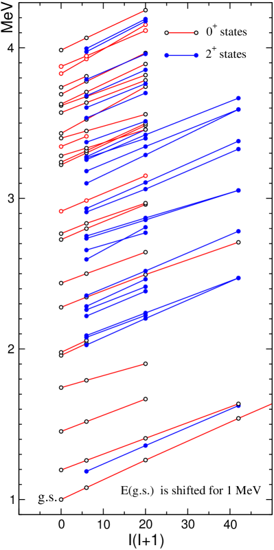
Figure 9: Collective bands based on the 0⁺ and 2⁺ excited states in ¹⁵⁸Gd as assigned from the DWBA fit of the angular distributions found from the (p,t) reaction as functions of the spin variable $I(I+1)$.

Within a rotational band, its members share almost the same MoI, i.e. only small, relatively smooth variations of the MoI value with increasing spin may occur, and this is emphasized by the straight lines in Fig. 9. The moments of inertia calculated through the slopes of these lines are listed in Table 2.

It can be expected that the MoI reflects the intrinsic structure of the rotational band, for which the pairing interaction is important. Fig. 10 demonstrates that the MoI magnitudes for most excited states in ¹⁵⁸Gd are larger than that of the g.s.. They are located in a region limited by the g.s. value and that of the first excited bands known from previous studies. Most of them have values close to that of the ground state MoI equal approximately to 37.5 MeV^-1. According to Ref. Bohr98 , vibrational bands have MoI that are typically a few percent larger than that of the g.s. band. More than half of the bands based on 0⁺ states reveal just this property. The bands with a significantly larger MoI are supposedly based on two-phonon states or having even more complicated phonon structure. The two-quasiparticle states with spins 2⁺ and higher can also be detected in the spectra, although the cross section for their excitation is expected to be weak. Due to the blocking effect, rotational bands built on such states may exhibit MoI 30 - 50% larger than that for the ground state band Bohr98 . Some bands have MoI lower than those of the g.s. Two of them are 2⁺ state bands, their MoI are only about 1% lower than that of the ground state. One band head at 1187.2 keV is a $\gamma$ - vibrational state. Five of the heads of such bands are 0⁺ states with the MoI between 31.1 and 37.4 MeV^-1, they are located above 3400 keV, much higher than twice the energy gap. Their structure is intriguing.

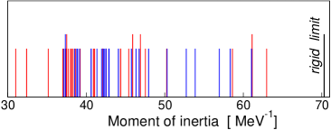
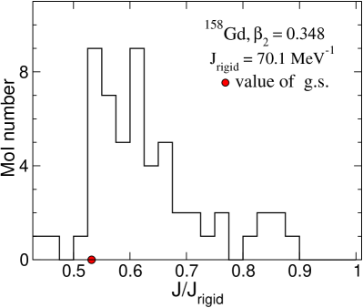
Figure 10: Top: The moments of inertia (MoI) as determined from the assigned collective bands. The moments of inertia for 0⁺ and 2⁺ states are shown by red and blue lines, respectively. Larger height represents the data known from previous studies.
Bottom: Distribution of number of the MoI values versus the dimensionless values $J/J_{rigid}$. The value of $J_{rigid}$ is evaluated according to Eq. (3). A sampling interval is 0.025.

It is well known that the nucleus in the lowest excited states has MoI values which do not exceed approximately 50% of the moment of inertia of a rigid rotator with the same nuclear mass. A part of the nucleons of the nucleus is not involved in the rotational motion due to the effect of the nucleon pairing, which leads to superfluid properties of nuclei in the ground and lower excited states. The moment of inertia for a statistically equilibrium rotation LLv5 can be approximated as the rigid body limit Sitenko14 ,

$$\frac{J_{rigid}}{\hbar^{2}}=\frac{2}{5}\frac{mA^{5/3}r_{0}^{2}}{\hbar^{2}}(1+0.32\beta_{2})~{}.$$ (3)

where a shape of spheroid with the deformation $\beta_{2}$ was assumed for the nucleus. For ¹⁵⁸Gd, the rigid-rotator MoI value (3) is about 70 MeV^-1. The standard deformation parameter $\beta_{2}$ describing mainly the nuclear shape is another important characteristic affecting the MoI magnitude. Due to the pairing effect, one can expect that the MoI magnitude deviates much from the rigid-rotator limit (3), namely, the MoI decreases by about 44%. Thus, the two factors - nuclear deformation and pairing - and, in addition, the centrifugal stretching can be considered as the main reasons of a significant increase of the MoI with increasing excitation energy, as compared to the ground state value. The largest value of the MoI is equal to 63 MeV^-1, that is, almost 90% of the rigid-body limit (3). The distribution of the MoI values relative to the rigid-rotator value (3) is shown in Fig. 10.

III.2 Statistical analysis of the 0⁺ and 2⁺ state sequences and possible $K$ symmetry breaking.

Sequences of states observed in the extended excitation energy interval in ¹⁵⁸Gd are considered to be long enough to perform statistical analysis even for one nucleus, see Table 3. The present analysis is triggered by the publication of Paar and Vorkapi Paa90 , which is devoted to the investigation of effects of the exact $K$ quantum number on the fluctuation properties of the energy spectra for 0⁺ and 2⁺ states in the SU(3) limit of the IBM. The $\Delta_{3}$ statistics Dys63 was used to obtain information about the long-range correlations of level spacings. In Ref. Paa90 , the $\Delta_{3}$ statistics for the pure sequence of the $0^{+}$ levels is close to the Wigner (chaotic) behavior while for the mixed sequence of all $2^{+}$ levels is close to the Poisson (regular) behavior (see also Ref. Gom11 ). The $\Delta_{3}$ statistics with the fixed $K$ sequences $(I=2,K=0)$ and $(I=2,K=2)$ return back to the Wigner distribution.

The sequences of states considered above as rotational bands look basically long enough to carry out the statistical analysis both for $K$ mixed sequences of 2⁺ and $4^{+}$ states and, separately, for the sub-sequences with $(I=2,K=0)$ and $(I=2,K=2)$ as well as for those with $(I=4,K=0)$, $(I=4,K=2)$ and $(I=4,K=4)$. The number of levels in all such sequences is shown in Table 3.

$I/K$	All	$K=0$	$K=2$	$K=4$
0+	37
2+	100	37	63
4+	90	37	28	25
All	227	74	92	25

Table 3: Number of levels included in the statistical analysis. They can be compared with the corresponding numbers at study of the isospin symmetry breaking in ³⁰P: 102 of all levels, 69 for $T=0$ and 33 for $T=1$.

The nearest neighbor-spacing distributions (NNSD) Wig65 ; Lev18 are applied to investigate the fluctuation properties of short-range correlations of the experimental spectra. The NNSDs are fitted by using the linear Wigner-Dyson approximation LWD with one parameter $w$ Mag18 ,

$$p_{\rm LWD}(s)=[a(w)+b(w)s]~{}\exp\left[-a(w)s-\frac{b(w)}{2}s^{2}\right],$$ (4)

where

$$a=\sqrt{\pi}~{}w~{}e^{w^{2}}~{}\mbox{erfc}(w)~{},\qquad b=\frac{\pi}{2}~{}e^{2w^{2}}~{}\mbox{erfc}^{2}(w)~{}.$$ (5)

$\mbox{erfc}(w)=1-\mbox{erf}(w)$, $\mbox{erf}(w)$ is the error function.

The LWD allows to obtain information on the quantitative measure of the Poisson regular and Wigner chaotic contributions, separately, in contrast to the heuristic Brody parameterization Bro73 with a fitting parameter which has not, in this respect, a clearly defined meaning. Results of fitting for two angular momenta, 0⁺ and 2⁺ are shown in Fig. 11 and in Table 4. For calculations of the experimental NNSDs, simple polynomials of low powers were used for fitting well the staircase cumulative level density obtained from experiments to get the so called unfolding (uniformed dimensionless) energy levels, see Ref. Lev18 for details. NNSDs for the spin 2⁺ with the fixed angular-momentum projections $K=0$ (c) and $2$ (d) have a Poisson-like structure, similar to the NNSD for 0⁺ state (a). The NNSD for the spin 2⁺ without fixing (“all K”) the angular momentum projection is shifted to the Wigner distribution. Fig. 12 and Table 4 show the results of the analysis for the spin $I=4$. The NNSDs have the Poisson-like structure for all sequences, except for the ($I=4$, $K=2$) one which demonstrates a noticeable shift towards the Wigner distribution.

$I^{\pi}$	$K$	$a$	$b$	$w$	$\chi^{2}_{2}$
0+	$0$	98.1	1.9	5.04	11.6%
2+	all $K$	58.1	41.9	0.66	14.9%
2+	0	98.2	1.8	5.2	9.8%
2+	2+	90.8	9.2	2.2	13.2%
4+	all $K$	82.3	17.7	1.4	17.7%
4+	0	98.2	1.8	5.1	8.9%
4+	2	76.2	23.8	1.1	16.5%
4+	4	98.2	1.8	5.2	14.0%

Table 4: Parameters $a$ and $b$ are one-parameter LWD approximation (4) within the Wigner-Dyson theory for the excited states 0⁺, for 2⁺ with all $K$, fixed $K=0$ and $K=2$ and for 4⁺ with all $K$, fixed $K=0$, $K=2$ and $K=4$ in ¹⁵⁸Gd. NNSD parameters for Poisson and Wigner contributions $a$ and $b$ are reduced to total 100%. Large $w$ ($w=\infty$) corresponds to Poisson and small $w$ ($w=0$) is related to the Wigner limits. The standard accuracies found by $\chi^{2}_{i}$ of the least-squares fittings are given in percent. A sampling interval is 0.2.

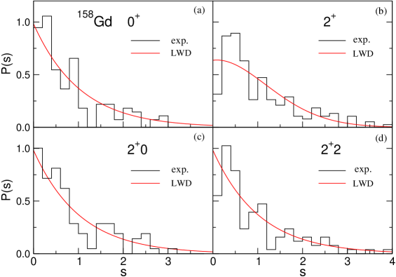
Figure 11: The nearest neighbor-spacing distributions for 0⁺ states (a) and for 2⁺ states with all projections $K$ (b), fixed $K=0$ (c) and $K=2$ (d) projections.

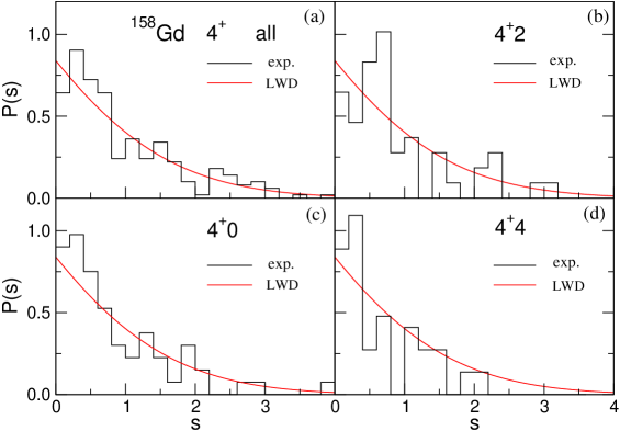
Figure 12: The nearest neighbor-spacing distributions for 4⁺ states with all projections $K$ (a), fixed $K=0$ (b), $K=2$ (c) and $K=4$ (d) projections.

Joining the sets of 0⁺ states in the rare earth and actinide nuclei, which became available from the rich data obtained during the last decades Lev94 ; Wir04 ; Lev09 ; Lev13 ; Lev15 ; Spi13 ; Mey06 ; Buc06 ; Bet09 ; Ili10 ; Spi18 ; Lev19 , demonstrate intermediate statistics between the Wigner and Poisson limits Lev18 . As shown in Ref. Lev18 the level spacing distributions for the collective 0⁺, 2⁺ and 4⁺ states mixing all $K$ in the actinide nuclei were found to be gradually shifted to the Poisson limit with increasing the spin Lev18 . In ¹⁵⁸Gd we observe a different behavior: practically a pure Poisson statistics for 0⁺ states and an essential shift to the Wigner distribution for 2⁺ states with all $K$. In the case of 4⁺ states we find the level spacing distribution close to the Poisson limit for a sequence that includes all $K$ and for the sub-sequences ($I=4,K=0$) and ($I=4,K=4$). However, the level spacing distribution for the sub-sequence $(I=4,K=2)$ demonstrates again a slight shift towards the Wigner limit.

The experimental results for the fixed $K$ projections in the case of 2⁺ as well as of 4⁺ states differ from the calculations performed in Ref. Paa90 . These results cannot be compared directly since the $\Delta_{3}$ statistics analysis has been performed for long correlations in Ref. Paa90 . However, from a general point of view, having a good quantum number $K$ one should expect a shift to the Wigner distribution in the sub-space of the fixed $K$ value for a given angular momentum $I$ with respect to the case of accounting for all $K$ BM98 ; BM12 ; LM19 . This is because of decreasing of the single-valued integral-motion numbers (conservation laws) due to a breaking of the axial symmetry in the sub-space versus its presence in the complete space. In such a sub-space, one finds more a system disordering or chaos . The arguments for this interpretation of the $K$-breaking are working well for the NNSDs in the case of actinide nuclei Mag18 ; LM19 . The present results for ¹⁵⁸Gd differ from those in Ref. Lev18 ; Mag18 and are not so clearly understood. Only the case of ($I$=4,$K=2$) can be considered as supporting to some extent this interpretation, see Fig. 12 (b) and Fig. 12 (a). Its NNSD is between the Wigner and Poisson limits, i.e. is not so pronounced as in actinide nuclei Mag18 ; LM19 . And Wigner’s contribution to the NNSD in this case (b) is much less   than Poisson one. As for the remaining sub-sequences with $(I=2,K=0)$ and $(I=2,K=2)$ as well as for sub-sequences with $(I=4,K=0)$ and $(I=4,K=4)$, they are strongly shifted to a regular Poisson distribution. Although the number of levels used in the analysis is limited, this affects only the accuracy of determining the Wigner and Poisson contributions. Such behavior might be interpreted as a $K$ symmetry breaking when $K$ is a good quantum number. That is a subject for further study in forthcoming work.

The effects of another symmetry breaking on the level statistics were studied experimentally in ²⁶Al Mit88 and ³⁰P Shr00 ; Shr04 . Statistical analyses have been performed taking into account the isospin quantum number $T$. The experimental distributions P(s) occurred to be equally far from Wigner and Poisson limits as for the ($I^{\pi};T$) sequences, and for the ($I^{\pi}$) sequences when the isospin quantum number $T$ is ignored. The reason for this behavior may be that, although sequences of different $T$ are not correlated if isospin describes an exact symmetry, even a small breaking of isospin symmetry may lead to similar fluctuation properties for ($I^{\pi};T$) and the ($I^{\pi}$) sequences Gom11 . According to theoretical calculations Dys62 and Pan81 in that case spectral fluctuations may be nearly independent of $T$. Probably similar situation is met also in the ¹⁵⁸Gd nucleus when $K$ is a good quantum number.

A puzzle is remaining why the NNSD for the mixed 2⁺ sequence demonstrates a shift to the Wigner distribution, cf. (b) with (a) in Fig. 11. The present analysis includes the states excited in the (p,t) reaction. According to previous studies Lev09 ; Lev13 ; Lev15 ; Buc06 ; Spi18 , the multiple 0⁺ states excited in the (p,t) reaction are found to be collective. This is perhaps not the case for 2⁺ states; the excitations of states of another nature are not excluded, though with a smaller cross section. To verify this assumption and to see how these states can influence on the results of statistical analysis, non-collective 2⁺ states from the compilation  Nic17 , not observed in the present (p,t) experiment, were included in the analysed sequence. The obtained P(s) turned out to be additionally shifted to the Wigner distribution in comparison with that shown in Fig. 11 (b). The presence of non-collective states in the sequence of 2⁺ states can be probably one of the reasons of such observed NNSD for 2⁺ states shifted to the Wigner limit as compared to that for 0⁺ and 4⁺ states. Non-collective levels are probably absent in the $(I=2,K=0)$ sequence and present in the $(I=2,K=2)$ one what is reflected in the Wigner-Poisson contributions.

IV IBM calculations

The structure of ¹⁵⁸Gd was investigated in the framework of the Interacting Boson Model. The traditional version of the IBM Iach87 does not make any distinction between protons and neutrons and uses only $\it{s}$ and $\it{d}$ bosons (with angular momentum L=0 and 2, respectively) as the main ingredients to describe the low-lying positive-parity states of even-even nuclei. Several other versions have been proposed over the years that include the addition of several other type of bosons, like $\it{p}$, $\it{f}$ and $\it{g}$ (with angular momentum L= 1, 3 and 4, respectively). In the last 20 years, new and detailed data have been measured with the (p,t) reaction and a considerable amount of states, especially 0⁺, have been found. One of the interpretation of this increased number of 0⁺ excitations was given by the IBM using the $\it{spdf}$ version of the model. The reason is that by coupling of two negative-parity bosons the model produces additional K^π=0⁺ states which have a N_pf=2 configuration. Such calculations have been performed in Refs. Zamfir01 ; Lev09 ; Lev13 ; Lev15 and have shown a rather good reproduction of the overall trend of electromagnetic and hadronic observables. This interpretation involves an increased contribution of the octupole degree of freedom in the low-lying structure of nuclei, which is in disagreement with a prediction of other theoretical models, for example, the Quasiparticle Phonon Model (QPM). The QPM indicates a moderate contribution of the octupole components in their wave functions while gives an increased weight of the pairing correlations Lo05 . Therefore, one needs experimental data concerning different type of observables in order to test properly the two predictions. The case of ¹⁵⁸Gd is one of the most promising examples for the following reason. In the rare-earth region, this is the only nucleus that has information both from the (p,t) transfer reaction and from a dedicated neutron inelastic scattering experiment aimed at measuring the lifetimes of the new 0⁺ excitations in (p,t) Lesh07 . Together with known transition probabilities of the lowest octupole states, we have a very fertile testing ground of the IBM predictions.

Therefore, we have performed calculations in the spdf IBM-1 framework using the Extended Consistent Q-formalism (ECQF) Casten01 . Although the equations employed by the model have been given in several papers, e.g. Refs. Zam01 ; Zam03 ; Zamfir01 ; Scholten01 , we briefly list them again below. The usual Hamiltonian is given by:

$$\hat{H}_{spdf}=\mathrm{\epsilon}_{d}\hat{n}_{d}+\mathrm{\epsilon}_{p}\hat{n}_{p}+\mathrm{\epsilon}_{f}\hat{n}_{f}+\mathrm{\kappa}(\hat{Q}_{spdf}\cdot\hat{Q}_{spdf})^{(0)}$$

$$+\alpha\hat{D}^{\dagger}_{spdf}\cdot\hat{D}_{spdf}~{},$$ (6)

where $\epsilon_{d}$, $\epsilon_{p}$, and $\epsilon_{f}$ are the boson energies and $\hat{n}_{p}$, $\hat{n}_{d}$, and $\hat{n}_{f}$ are the boson number operators. We mention that one of the ingredients that was shown to improve the transfer calculations, namely the inclusion of the octupole term in the Hamiltonian Lev13 ; Lev15 , was omitted in the present calculations since we preferred to maintain the form of the Hamiltonian given in Ref. Zamfir01 . $\hat{D}_{spdf}$ is introduced in the Hamiltonian in order to connect states with no ($pf$) content with those having $(pf)^{2}$ components, and it has a very small strength as shown in Table 5. The form of this operator is taken as earlier, see Refs. Zam01 ; Zam03 ,

$$\hat{D}_{spdf}=-2\sqrt{2}[{p}^{\dagger}\tilde{d}+{d}^{\dagger}\tilde{p}]^{(1)}+\sqrt{5}[{s}^{\dagger}\tilde{p}+{p}^{\dagger}\tilde{s}]^{(1)}$$ (7)

$$+\sqrt{7}[{d}^{\dagger}\tilde{f}+{f}^{\dagger}\tilde{d}]^{(1)}~{}.$$

For the quadrupole operator one has Kusnezov01 :

$$\hat{Q}_{spdf}=\hat{Q}_{sd}+\hat{Q}_{pf}=$$

$$(\hat{s}^{\dagger}\tilde{d}+\hat{d}^{\dagger}\hat{s})^{(2)}+\chi^{(2)}_{sd}(\hat{d}^{\dagger}\tilde{d})^{(2)}+\frac{3\sqrt{7}}{5}[(p^{\dagger}\tilde{f}+f^{\dagger}\tilde{p})]^{(2)}$$

$$-\frac{9\sqrt{3}}{10}(p^{\dagger}\tilde{p})^{(2)}-\frac{3\sqrt{42}}{10}(f^{\dagger}\tilde{f})^{(2)}$$ (8)

The quadrupole electromagnetic transition operator is defined by

$$\hat{T}(E2)=e_{2}\hat{Q}_{spdf}$$ (9)

where $e_{2}$ represents the boson effective charge.

Table 5: The $spdf$-IBM parameters used in the present calculations. The parameters of the Hamiltonian are taken from Ref. Zamfir01 , while the others are determined from a fitting procedure on the corresponding experimental data.

Parameters		Nucleus
		158Gd	160Gd
	$\epsilon_{d}$ (MeV)	0.315	0.213
	$\epsilon_{p}$ (MeV)	4.0	4.0
Hamiltonian	$\epsilon_{f}$ (MeV)	0.95	1.3
	$\kappa$ (MeV)	-0.02	-0.02
	$\chi_{sd}$	-0.91	-0.53
	$\alpha$ (MeV)	0.0005	0.0005
	$e_{2}$ (eb)	0.132	0.132
EM transition	$e_{1}$ (eb1/2)	0.053	0.053
operators	$\chi_{sp}$	1.07	1.07
	$\chi_{df}$	-0.55	-0.55
	$\alpha_{\nu}$ (mb/sr)	0.008
Transfer operator	$\alpha_{p}$ (mb/sr)	4.22
	$\alpha_{f}$ (mb/sr)	-0.4

Figure 13: Comparison between the experimental and $spdf$-IBM calculations for the 0⁺, 2⁺, and 4⁺ states up to 4.3 MeV. The levels with a double-octupole character in the IBM are marked with a star.

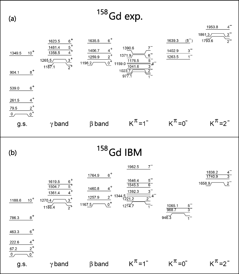
Figure 14: Experimental (a) and $spdf$-IBM (b) level scheme of ¹⁵⁸Gd. The g.s., $\gamma$, and $\beta$ band are shown for the positive-parity states, while the K^π=0^-, 1^- and 2^- octupole bands are presented for the negative-parity levels.

Since the IBM yields the increased octupole correlations in the structure of even-even nuclei, it is essential to calculate the $E1$ transition strengths and to compare the results with the experimental values. For the $E1$ operator in the IBM one has

$$\hat{T}(E1)=e_{1}[\chi_{sp}^{(1)}({s}^{\dagger}\tilde{p}+{p}^{\dagger}\tilde{s})^{(1)}+({p}^{\dagger}\tilde{d}+{d}^{\dagger}\tilde{p})^{(1)}$$

$$+\chi_{df}^{(1)}({d}^{\dagger}\tilde{f}+{f}^{\dagger}\tilde{d})^{(1)}]~{},$$ (10)

where $e_{1}$ is the effective charge for the $E1$ transitions and $\chi_{sp}^{(1)}$ and $\chi_{df}^{(1)}$ are two model parameters.

The final equation which we need is the one for the transfer operator. Previously, only the last term in Eq. (11) was used Scholten01 , but recent successful calculations Lev13 ; Lev15 have shown that it is imperative to include also at least one term related to the negative-parity bosons

$$\hat{P}^{(0)}_{\nu}=(\alpha_{p}\hat{n}_{p}+\alpha_{f}\hat{n}_{f})\hat{s}+$$

$$+\alpha_{\nu}\left(\Omega_{\nu}-N_{\nu}-\frac{N_{\nu}}{N}\hat{n}_{d}\right)^{\frac{1}{2}}\left(\frac{N_{\nu}+1}{N+1}\right)^{\frac{1}{2}}\hat{s}$$ (11)

where $\Omega_{\nu}$ is the pair degeneracy of neutron shells, $N_{\nu}$ is the number of neutron pairs, $N$ is the total number of bosons, and $\alpha_{p}$, $\alpha_{f}$, and $\alpha_{\nu}$ are constant parameters.

Schematic $\it{spdf}$-IBM calculations have been performed in Ref. Zamfir01 shortly after limited data on 0⁺ states in ¹⁵⁸Gd were obtained in the (p,t) experiment Lesh02 . With more data on hand, we proceed to investigate not only the distribution in energy of the 0⁺ states, but also the detailed structure of ¹⁵⁸Gd, including the energies of the low-lying levels, the transition probabilities in the first bands and the distribution in transfer intensity of the 0⁺ states up to 4.5 MeV. To perform the calculations we employed the OCTUPOLE code Kusnezov02 to diagonalize the Hamiltonian in Eq.(6). Up to three negative-parity bosons were allowed in the calculations and the parameters of the Hamiltonian were taken from Ref. Zamfir01 , while the ones for the transition and transfer operators were fitted to the available experimental information. The IBM parameters are summarized in Table 5.

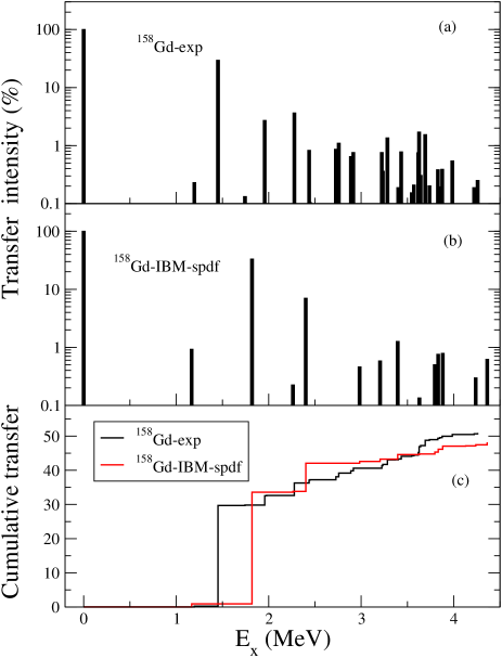
Figure 15: Comparison between the experimental (a) and $spdf$-IBM calculations (b) for the transfer intensity in ¹⁵⁸Gd. Cumulative strength as a function of energy is given in (c) for experiment (black) and calculations (red).

The authors of Ref. Zamfir01 have presented a comparison of the experimental energy levels with the corresponding ones calculated in the $spdf$-IBM framework. Their work concentrated mainly on the reproduction of the 0⁺ states and it was for the first time when the model predicted an increased number of 0⁺ levels, close to the experimentally observed one. The contribution of the octupole degree of freedom was crucial, the model describing twelve 0⁺ states up to around 3.5 MeV, where the experimental data were available at that time. In Fig. 13 we present the complete results of the IBM calculations for the 0⁺, 2⁺, and 4⁺ states up to 4.3 MeV in comparison with the values obtained in the present experiment. It is clear that the experiment has revealed a greater number of states that can be produced by the IBM, irrespective of spin. The experiment provides 36 (0⁺), 95 (2⁺), and 64 (4⁺) states, while the IBM gives only 17 (0⁺), 20 (2⁺), and 19 (4⁺) states. Some of these levels having a double-octupole character are marked with a star in Fig. 13. It is clear that this version of the IBM is satisfactorily describing the low energy part of the spectra, but is not so successful in describing the spectra at higher excitation energies, and a more complicate version should be used or other models have to be considered in order to elucidate the structure of ¹⁵⁸Gd.

In Fig. 14 we compare the energy levels of the lowest positive- and negative-parity bands, using the data from the latest evaluation in ENSDF Nic17 . One observes a rather good reproduction of the experimental data, especially of the positive-parity states. For the negative-parity levels, the calculations show a band order with K^π=0^-, 1^- and 2^-, while in the experiment the order is K^π=1^-, 0^- and 2^-. This effect was previously noticed in the IBM calculations Cottle01 and it was related to the fractional filling of the proton and neutron valence shells. The ordering can be improved in the IBM by introducing another term in the calculations that will lower the K^π=1^- band in energy Cottle01 . However, since we try to keep the calculations as close as possible to the ones in Ref. Zamfir01 , this term was not included in the Hamiltonian, Eq. (6).

The results for the transfer intensity calculated in the IBM by using Eq.(11) are compared with the experimental data in Fig. 15. As noted above, the IBM does not reproduce the number of 0⁺ states obtained in the present experiment: 17 excited 0⁺ levels in the IBM calculations are found versus the 36 experimental 0⁺ excitations in the energy region under the consideration. It is clear that some of the observed 0⁺ excitations are having a two quasi-particle nature and are, therefore, outside of the model space. Thus, detailed microscopic calculations are needed to reproduce the structure of all these states. Nevertheless, we look also at the transfer intensity produced by the IBM model in order to see how much the observed strength may have a collective origin. In Fig. 15, (a) and (b), we present the experimental and calculated transfer strength, respectively. One can see that the IBM does give a reasonable reproduction of the experimental data for the transfer intensity. The first excited 0⁺ state has 0.2$\%$ of the ground strength in the experiment and 0.9$\%$ in the calculations, while the second excited 0⁺ state has about 30$\%$ and 34$\%$ in experiment and calculations, respectively. For higher-lying excitations, one obtains about 20$\%$ in the experiment, and amount to about 14$\%$ in the IBM. The distribution of the transfer strength is better illustrated in Fig. 15 (c), where we compare the experimental and calculated cumulative transfer. It is clear that the model reproduces the experimental data up to about 3.5 MeV, and starts to underestimate it at higher excitation energy. It will be interesting to obtain experimental data for energies even higher than 4.3 MeV in future experiments to better compare the distribution in energy and transfer strengths of the higher-lying states.

Table 6: Experimental and calculated $E1$ and $E2$ transition probabilities in ¹⁵⁸Gd. The parameters of the $E1$ and $E2$ operators are fitted to the experimental data available Nic17 .

Kπ	Ei (keV)	Ji	Jf	Exp. (W.u.)	IBM (W.u.)
$E2$ transitions
g.s	80	2+	g.s.	198(5)	198
	261	4+	2${}^{+}_{1}$	290(4)	280
	904	8+	6${}^{+}_{1}$	330(30)	308
	1350	10+	8${}^{+}_{1}$	340(30)	304
$\beta$-band	1196	0+	2${}^{+}_{1}$	1.17${}^{+4.18}_{-0.13}$	4.79
	1260	2+	4${}^{+}_{1}$	1.39(15)	3.25
		2+	2${}^{+}_{1}$	0.079(14)	0.47
		2+	0${}^{+}_{1}$	0.31(4)	0.97
	1407	4+	2${}^{+}_{\beta}$	456${}^{+912}_{-67}$	180
		4+	2${}^{+}_{\gamma}$	12.8${}^{+25.6}_{-1.9}$	1.2
		4+	6${}^{+}_{1}$	3.16${}^{+6.32}_{-0.46}$	3.66
		4+	4${}^{+}_{1}$	0.37${}^{+0.74}_{-0.05}$	0.005
		4+	2${}^{+}_{1}$	1.32${}^{+2.64}_{-0.19}$	1.01
$\gamma$-band	1187	2+	4${}^{+}_{1}$	0.27(4)	0.12
		2+	2${}^{+}_{1}$	6.0(7)	5.65
		2+	0${}^{+}_{1}$	3.4(3)	2.23
	1266	3+	4${}^{+}_{1}$	1.77${}^{+3.27}_{-0.19}$	3.29
		3+	2${}^{+}_{1}$	3.5${}^{+6.47}_{-0.37}$	4.61
	1358	4+	2γ	113${}^{+166}_{-13}$	99
		4+	6${}^{+}_{1}$	$>$0.95	0.07
		4+	4${}^{+}_{1}$	7.3${}^{+10.7}_{-0.9}$	6.9
		4+	2${}^{+}_{1}$	1.13${}^{+1.65}_{-0.14}$	0.43
$E1$ transitions
1-	977	1-	2${}^{+}_{1}$	9.7${}^{+12.7}_{-1.1}$ $\cdot$10-5	5.2$\cdot$10-5
		1-	0${}^{+}_{1}$	9.8${}^{+12.8}_{-1.1}$ $\cdot$10-5	29.2$\cdot$10-5
	1042	3-	4${}^{+}_{1}$	2.9(8)$\cdot$10-4	3.3$\cdot$10-4
		3-	2${}^{+}_{1}$	3.3(10)$\cdot$10-4	0.8$\cdot$10-4
	1159	4-	4${}^{+}_{1}$	9.3${}^{+18.6}_{-1.2}$ $\cdot$10-5	12.1$\cdot$10-5
	1176	5-	6${}^{+}_{1}$	5.9${}^{+6.7}_{-0.7}$ $\cdot$10-4	10.9$\cdot$10-4
		5-	4${}^{+}_{1}$	7.4${}^{+8.4}_{-0.8}$ $\cdot$10-4	0.72$\cdot$10-4
0-	1264	1-	2${}^{+}_{1}$	6.4(21)$\cdot$10-3	9.5$\cdot$10-3
		1-	0${}^{+}_{1}$	3.5(12)$\cdot$10-3	4.3$\cdot$10-3
	1403	3-	4${}^{+}_{1}$	1.6(3)$\cdot$10-2	1.0$\cdot$10-2
		3-	2${}^{+}_{1}$	1.2${}^{+0.2}_{-0.23}$ $\cdot$10-2	0.8$\cdot$10-2
2-	1794	2-	3${}^{+}_{\gamma}$	5.0${}^{+10.0}_{-0.6}$ $\cdot$10-5	167$\cdot$10-5
		2-	2${}^{+}_{\gamma}$	8.6${}^{+17.2}_{-1.1}$ $\cdot$10-5	294$\cdot$10-5
		2-	2${}^{+}_{1}$	1.8${}^{+35.0}_{-0.2}$ $\cdot$10-7	5410$\cdot$10-7

Finally, we look at the reduced matrix elements that can provide a better insight if the relevant degrees of freedom are taken into account. For the case of ¹⁵⁸Gd, most of the lifetimes have been measured for the low-lying states, with both positive and negative parity Nic17 . Therefore, an impressive amount of B(E1) and B(E2) values is available to be compared with the theoretical calculations. In Table 6 we present the IBM results for the $E1$ and $E2$ transition probabilities for the g.s, $\beta$, and $\gamma$ band, as well as for the K^π=0^-, 1^- and 2^- octupole bands. The model reproduces the gross features of the low-lying states in ¹⁵⁸Gd, but a closer inspection reveals that there are some severe discrepancies with respect to the experimental data. The $E1$ transitions in the K^π=2^- band are found to be much stronger than in the experiment, although the experimental uncertainty is quite large. The same situation happens for the $E1$ transition from the 0${}_{2}^{+}$ state to the 1${}_{1}^{-}$. However, most of the transitions are obtained within less than a factor of five as compared to the experimental data. For the higher-lying 0⁺ states, the (n,n’$\gamma$) experiment has revealed a low $E1$ transition strength up to around 3 MeV Lesh07 . Since the double-octupole states play a major role in the IBM, it is not surprising that many of these states are predicted with a relatively high $E1$ transition strength. Therefore, we conclude that although the low-lying structure of ¹⁵⁸Gd is reasonable well reproduced by the IBM calculations, the theory does not reproduce in details the nature of the higher-lying 0⁺ states.

IV.1 Conclusion

A proper study of excited states with energies up to 4.3 MeV in the deformed nucleus ¹⁵⁸Gd was performed by a high-resolution (p,t) transfer reaction using the Q3D spectrograph. In total, 206 excited states of positive parity and 20 of negative parity were identified and many of them were observed for the first time. The high resolution, background-free experiment allowed, in fact, a quasi-complete determination of levels up to excitation energies with a high level density. The collective nature of these states is provided by the selectivity of the (p,t) reaction to the structure of the densely populated final states. To assign spin and parity to the states, angular distributions were measured and compared to the predictions of coupled-channel DWBA calculations. Many rotational bands built upon the low-lying band heads excited in our experiment were identified. Moments of inertia calculated using energies of such bands are analysed. The large sets of states with the same spin-parity allowed to carry out their statistical analysis. Such an analysis is performed for the 0⁺ and 2⁺ states sequences including all K-values and for well-determined projections K of the angular momentum. We intended to obtain confirmation of theoretical predictions about the chaotic nature of sequences with a well-determined projection $K$ of the angular momentum. However, all but one analysed NNSDs indicate clearly on the regular nature. Although the number of levels used in the analysis is limited, which affects the accuracy of determination of the Wigner and Poisson contributions, we interpreted this behavior as an indication of the $K$ symmetry breaking with $K$ being a good quantum number. More detailed analysis of such data for the rare-earth and actinide nuclei is a subject for further study in forthcoming work. The structure of ¹⁵⁸Gd was investigated in the framework of the Interacting Boson Model using the $spdf$ version of the model. The calculated energies of the low-lying levels, their transition probabilities in the lowest bands and their distributions in the transfer intensity of 0⁺ states are in rather good agreement with the experiment. We found clear signatures to go beyond the simplest spdf version of the IBM in describing the complete data. The description of such rich experimental data by more sophisticated, (semi)microscopical theoretical models, is of considerable interest.

V Acknowledgments

We are grateful to the members of the YMKB collaboration for access to the ¹⁵⁸Gd data, and thank Dr. Deseree A. Meyer (Brittingham) for useful discussions. We thank also the operators at MLL for excellent beam conditions. The work was supported in part by the Romanian project PN 18090102F2. This work was supported in part also by the budget program ”Support for the development of priority areas of scientific researches”, the project of the Academy of Sciences of Ukraine, Code 6541230.

References

- (1) R. C. Greenwood, C. W. Reich, H. A. Baader, H. R. Koch, D. Breitig, O. W. B. Schult, B. Fogelberg, A. Backlin, W. Mampe, T. von Egidy, E. Schreckenbach, Nucl. Phys. A304, 327 (1978).
- (2) H. G. Börner, M. Jentschel, N. V. Zamfir, R. F. Casten, M. Krticka, and W. Andrejtscheff, Phys. Rev. C59, 2432 (1999).
- (3) L. I. Govor, A. M. Demidov, I. V. Mikhailov, Physics of Atomic Nuclei 64, 1254 (2001).
- (4) A. F. Kluk, Noah R. Johnson, and J. H. Hamilton, Phys. Rev. C10, 1966 (1974).
- (5) H. Pitz, U. E. P. Berg, R. D. Heil, U. Kneissl, R. Stock, C. Wesselborg, P. Von Brentano, Nucl. Phys. A492, 411 (1989).
- (6) M. Sugawara, H. Kusakari, T. Morikawa, H. Inoue, Y. Yoshizawa, A. Virtanen, M. Piiparinen, T. Horiguchi, Nucl. Phys. A—bf557, 653 (1993)
- (7) S. R. Lesher, A. Aprahamian, L. Trache, A. Oros-Peusquens, S. Deyliz, A. Gollwitzer, R. Hertenberger, B. D. Valnion, G. Graw, Phys.Rev. C 66, 051305(R)(2002).
- (8) B. Ackermann, H. Baltzer, K. Freitag, C. Gunther, P. Herzog, J. Manns, U. Muller, R. Panlsen, P. Sevenich, T. Weber, B. Will, J. de Boer, G. Graw, A. I. Levon, M. Loewe, A. Losch, E. Muller-Zanotti, Z.Phys. A350, 13 (1994).
- (9) H. Baltzer, J. de Boer, A. Gollwitzer, G. Graw, C. Günther, A. I. Levon, M. Loewe, H. J. Maier, J. Manns, U. Müller, B. D. Valnion, T. Weber, and M. Würkner, Z. Phys. A356, 13 (1996)
- (10) A. I. Levon, J. de Boer, G. Graw, R. Hertenberger, D. Hofer, J. Kvasil, A. Lösch, E. Müller-Zanotti, M. Würkner, H. Baltzer, V. Grafen, and C. Günther, Nucl. Phys. A576, 267 (1994).
- (11) H.-F. Wirth, G. Graw, S. Christen, D. Cutoiu, Y. Eisermann, C. Günther, R. Hertenberger, J. Jolie, A. I. Levon, O. Möller, G. Thiamova, P. Thirolf, D. Tonev, and N. V. Zamfir, Phys. Rev. C 69, 044310 (2004).
- (12) A. I. Levon, G. Graw, Y. Eisermann, R. Hertenberger, J. Jolie, N. Yu. Shirikova, A. E. Stuchbery, A. V. Sushkov, P. G. Thirolf, H.-F. Wirth, and N. V. Zamfir, Phys. Rev. C 79, 014318 (2009).
- (13) A. I. Levon, G. Graw, R. Hertenberger, S. Pascu, P. G. Thirolf, H.-F. Wirth, and P. Alexa, Phys. Rev. C 88, 014310 (2013).
- (14) A. I. Levon, P. Alexa, G. Graw, R. Hertenberger, S. Pascu, P. G. Thirolf, H.-F. Wirth, Phys.Rev. C 92, 064319 (2015).
- (15) M. Spieker, D. Bucurescu, J. Endres, T. Faestermann, R. Hertenberger, S. Pascu, S. Skalacki, S. Weber, H.-F. Wirth, N.V. Zamfir, and A. Zilges, Phys. Rev. C 88, 041303(R) (2013).
- (16) D. A. Meyer, V. Wood, R. F. Casten, C. R. Fitzpatrick, G. Graw, D. Bucurescu, J. Jolie, P. von Brentano, R. Hertenberger, H.-F. Wirth, N. Braun, T. Faestermann, S. Heinze, J. L. Jerke, R. Krücken, M. Mahgoub, O. Möller, D. Mücher, and C. Scholl, Phys. Rev. C 74, 044309 (2006); J. Phys. G31, S1399 (2005); Phys. Lett. B638, 44 (2006).
- (17) D. Bucurescu, G. Graw, R. Hertenberger, H.-F. Wirth, N. Lo Iudice, A. V. Sushkov, N. Yu. Shirikova, Y. Sun, T. Faestermann, R. Krücken, M. Mahgoub, J. Jolie, P. von Brentano, N. Braun, S. Heinze, O. Möller, D. Mücher, C. Scholl, R.F. Casten, D.A. Meyer, Phys. Rev. C 73, 064309 (2006).
- (18) L. Bettermann, S. Heinze, J. Jolie, D. Mücher, O. Möller, C. Scholl, R. F. Casten, D. A. Meyer, G. Graw, R. Hertenberger, H.-F. Wirth, and D. Bucurescu, Phys. Rev. C 80, 044333 (2009).
- (19) G. Ilie, R. F. Casten, P. von Brentano, D. Bucurescu, T. Faestermann, G. Graw, S. Heinze, R. Hertenberger, J. Jolie, R. Krücken, D. A. Meyer, D. Mücher, C. Scholl, V. Werner, R. Winkler, and H.-F. Wirth, Phys. Rev. C 82, 024303 (2010).
- (20) M. Spieker, S. Pascu, D. Bucurescu, T. M. Shneidman, T. Faestermann, R. Hertenberger, H.-F. Wirth, N. V. Zamfir, and A. Zilges, Phys. Rev. C 97, 064319 (2018).
- (21) A. I. Levon, D. Bucurescu, C. Costache, T. Faestermann, R. Hertenberger, A. Ionescu, R. Lica, A. G. Magner, C. Mihai, R. Mihai, C. R. Nita, S. Pascu, K. P. Shevchenko, A. A. Shevchuk, A. Turturica, and H.-F. Wirth, Phys. Rev. C100, 034307 (2019).
- (22) F. Iachello and A. Arima, The Interecting Boson Model (Cambridge University Press, Cambridge, 1987)
- (23) R. F. Casten and D. D. Warner, Rev. Mod. Phys. 60 389 (1988) and references therein.
- (24) N. V. Zamfir and D. Kusnezov, Phys. Rev. C 63, 054306 (2001).
- (25) N. V. Zamfir and D. Kusnezov, Phys. Rev. C 67, 014305 (2003).
- (26) K. Hara and Y. Sun, Int. J. Mod. Phys. E4, 637 (1995).
- (27) Y. Sun, A. Aprahamian, J.-Y. Zhang, C.-T. Lee, Phys.Rev. C 68, 061301(R)(2003).
- (28) V. G. Soloviev, Theory of Atomic Nuclei: Quasiparticles and Phonons (Inst.Phys., Bristol, Philadelphia, 1992).
- (29) V. G. Soloviev, A. V. Sushkov, and N. Yu. Shirikova, Nucl. Phys. 568, 244 (1994); J. Phys. G: Nucl. Part. Phys. 20, 113 (1994); Phys. Rev. C 51, 551 (1995); Phys. At. Nucl. 59, 51 (1996); Phys. At. Nucl. 60, 1599 (1997).
- (30) N. Lo Iudice, A. V. Sushkov, N. Yu. Shirikova, Phys.Rev. C70, 064316 (2004).
- (31) N. Lo Iudice, A. V. Sushkov, and N. Yu. Shirikova, Phys. Rev. C 72, 034303 (2005).
- (32) Murat Gerceklioglu, Phys. Rev. C 82, 024306 (2010).
- (33) H.-F. Wirth, Ph.D. thesis, Technische Universitat Munchen, 2001 (unpublished), https://mediatum.ub.tum.de/602907.
- (34) F. Riess, Beschleunigerlaboratorium München, Annual Report, 1991, p.168.
- (35) P. D. Kunz, computer code CHUCK3, University of Colorado, unpublished.
- (36) F. D. Becchetti and G. W. Greenlees, Phys. Rev. 182, 1190 (1969).
- (37) E. R. Flynn, D. D. Amstrong, J. G. Beery, and A. G. Blair, Phys. Rev. 182, 1113 (1969).
- (38) R. C. Greenwood, M. H. Putnam, K. D. Watts, Nucl. Instrum. Methods Phys. Res. A378, 312 (1996).
- (39) S. R. Lesher, J. N. Orce, Z. Ammar, C. D. Hannant, M. Merrick, N. Warr, T. B. Brown, N. Boukharouba, C. Fransen, M. Scheck, M. T. McEllistrem, and S. W. Yates, Phys. Rev C76, 034318 (2007).
- (40) N. Nica, Nucl. Data Sheets 141, 1 (2017)
- (41) F. D. Becchetti and G. W. Greenlees, in Proceedings of the Third International Symposium. on Polarization Phenomena in Nuclear Reactions,Madison, 1970, edited by H. H. Barshall and W. Haeberli (University of Wisconsin Press, Madison, 1971).
- (42) A. Bohr and B. R. Mottelson, Nuclear Structure (World Scientific, Singapore, 1998), Vol. 2.
- (43) D. J. Rowe, Nuclear Collective Motion: Models and Theory (University of Toronto, Canada, WORLD Science, 2010).
- (44) L. D. Landau and E. M. Lifshitz, Statistical Physics (Oxford, Pergamon 1975).
- (45) A. G. Sitenko and V.M. Tartakovsky, Lectures on the Theory of the Nucleus, edited by P. J. Shepherd (Department of Physics, University of Exeter, Pergamon Press, 2014).
- (46) V. Paar and D. Vorkapić, Phys.Rev. C41, 2397 (1990).
- (47) F. J. Dyson, M. L. Mehta, J. Math. Phys. 4, 701 (1963).
- (48) J. M. G. Gómez, K. Kar, V. K. B. Kota, R. A. Molina, A. Relaño, J. Retamosa, Phys.Reports 499, 103 (2011).
- (49) E. P. Wigner, in: C.E. Porter (Ed.), Statistical Theories of Spectra: Fluctuations, Academic Press, New York, 1965, p. 199.
- (50) A. I. Levon, A. G. Magner, and S. V. Radionov, Phys. Rev. C97, 044305 (2018).
- (51) A. G. Magner, A. I. Levon and S. V. Radionov, Eur. Phys. J. A54, 214 (2018)
- (52) T. A. Brody, Lett. Nuovo Cimento 7, 482 (1973).
- (53) A. Bohr and B. R. Mottelson, Nuclear Structure (World Scientific, Singapore, 1998), Vol. 1.
- (54) J. P. Blocki and A. G. Magner, Phys. Rev. C, 85, 064311 (2012).
- (55) A. I. Levon and A. G. Magner, Nucl. and Energy Phys., 20(2), 111 (2019).
- (56) V. Zelevinsky, B. A. Brown, N. Frazier, and M. Horoi, Rev. Rept., 276, 85 (1996).
- (57) G. E. Mitchell, E. G. Bilpuch, P. M. Endt, J. F. Shriner Jr., Phys. Rev. Lett. 61, 1473 (1988).
- (58) J. F. Shriner Jr., C. A. Grossmann, G. E. Mitchell, Phys. Rev. C62, 054305 (2000).
- (59) J. F. Shriner Jr., G. E. Mitchell, B. A. Brown, Phys. Lett. B586, 232 (2004).
- (60) F. J. Dyson, J. Math. Phys. 3, 1191 (1962).
- (61) A. Pandey, Ann. Phys. (N.Y.) 134, 110 (1981).
- (62) N. V. Zamfir, J. Y. Zhang, and R. F. Casten, Phys. Rev. C66, 057303 (2002).
- (63) D. Kusnezov, J. Phys. A23, 5673 (1990).
- (64) O. Scholten, F. Iachello, and A. Arima, Ann. Phys. 115, 325 (1978).
- (65) D. Kusnezov, computer code OCTUPOLE (unpublished).
- (66) P. D. Cottle and N. V. Zamfir, Phys. Rev. C54, 176 (1996).