Many-body scar state intrinsic to periodically driven system: Rigorous results
Abstract
The violation of the Floquet version of eigenstate thermalization hypothesis is systematically discussed with realistic Hamiltonians. Our model is based on the PXP type interactions without disorder. We exactly prove the existence of many-body scar states in the Floquet eigenstates, by showing the explicit expressions of the wave functions. Using the underlying physical mechanism, various driven Hamiltonians with Floquet-scar states can be systematically engineered.
In the past few decades, significant progress have been made in the in-depth understanding of the thermalization phenomenon in isolated systems Popescu et al. (2006); Goldstein et al. (2006); Goold et al. (2016); Yukalov (2011); Nandkishore and Huse (2015); D’Alessio et al. (2016); Gogolin and Eisert (2016); Mori et al. (2018). Thermalization is a fundamental phenomenon in physics, which is directly connected to Arrow of time in the sense of thermodynamics. In addition, it provides the underlying fundamental mechanism to validate the framework of statistical mechanics.
The eigenstate thermalization hypothesis (ETH) is one of the most important keywords in this subject for static systems, because if it holds the thermodynamic property in the isolated systems is consistently explained Reimann (2015); Deutsch (2018, 1991); Srednicki (1994). The ETH states that any single eigenstate is thermalized in the sense that an expectation value of any local observable is equal to the value calculated by the canonical ensemble with the corresponding temperature. When a periodic driving is applied to the system, the system generally heats up. In this case, the standard ETH is replaced by another hypothesis known as the Floquet ETH, which states that any single Floquet eigenstate is thermalized with an infinite temperature D’Alessio and Polkovnikov (2013); D’Alessio and Rigol (2014); Lazarides et al. (2014); Kuwahara et al. (2016); Mori et al. (2016). Both the ETH and the Floquet ETH have been intensively studied, and the affirmative results of many numerical simulations corroborate their validity, as long as the system is nonintegrable Kim et al. (2014); Mondaini et al. (2016); Mondaini and Rigol (2017); D’Alessio and Rigol (2014); Mori et al. (2016); Haldar et al. (2019). However, exceptions exist for both the ETH and the Floquet ETH. The most common example is the many-body localization, which is a phenomenon driven by disorder Nandkishore and Huse (2015); Ponte et al. (2015a, b). In the system exhibiting such phenomena, essentially all eigenstates are nonthermal states, which are protected by an extensive number of emergent local integrals of motion.
Recently, a new type of violation of the ETH has been found in the PXP model in the framework of many-body scar state Turner et al. (2018a, b); Moudgalya et al. (2018); Ho et al. (2019); Khemani et al. (2019); James et al. (2019); Choi et al. (2019). The PXP model is an effective model derived from the transverse Ising model that describes the experimental setup of a chain of Rydberg atoms Bernien et al. (2017). The many-body scar states have been numerically proposed as nonthermal eigenstates which consistently explain the long-time oscillations observed in experiments Bernien et al. (2017); Ho et al. (2019); Choi et al. (2019). In addition, Lin and Motrunich found the explicit expressions for several nonthermal eigenstates using the matrix product form Lin and Motrunich (2019). This work has rigorously ensured the existence of many-body scars in this system and has made their structure clearer. An intriguing nature is the absence of a local integral of motion, which is in stark contrast to the conventional theories on the breakdown of the thermalization such as the many-body localized and the integrable systems.
Very recently, a similar violation of the Floquet ETH has been numerically reported in a random unitary time-evolution Pai and Pretko (2019); Khemani and Nandkishore (2019) that models the Fracton dynamics Nandkishore and Hermele (2019); Pai et al. (2019). In this study, the unitary dynamics was randomly chosen, while the translational symmetry and several conservation laws were retained. The study numerically indicated that the Floquet operator has Floquet many-body scar states that imply nonthermal eigenstates of the Floquet operator. Because this is an important numerical indication, several questions should follow: (i) Can such a scar exist in a systematic Hamiltonian? If yes, what is the possible mechanism? (ii) Can we construct exact expressions for Floquet scar states, as was done for the scar states in the PXP model? Addressing these questions is indispensable for an in-depth understanding of the general structure of scar states, as well as for future experimental realization.
In this paper, we rigorously discuss the violation of the Floquet ETH in a systematic Hamiltonian. Our model is based on the PXP type interactions without disorder. Then, we rigorously prove the existence of the many-body Floquet scar states by deriving the explicit expressions of the eigenstates. Through the derivation of the wave functions, underlying mechanisms to have the Floquet scar states is clarified in this model. In addition, this mechanism enables us to engineer various Hamiltonians with Floquet scar states. Since our model is based on PXP type of interactions Bernien et al. (2017); Potirniche et al. (2017), simple cases of our Floquet scar states are experimentally feasible. By contrast, other eigenstates should satisfy the Floquet ETH. We numerically demonstrate that a quantum state usually relaxes to a state with infinite temperature in our system, while our Floquet scar state exhibits persistent oscillations which never decay.
Floquet-intrinsic many-body scar state.—
Let be a time-dependent many-body Hamiltonian, which is periodic in time with the period . The Floquet operator for a single period is given by
| (1) |
where is a time-ordering operator. We set to be unity. For simplicity, we consider the following time-dependence in the Hamiltonian:
| (4) |
Hereinafter, we assume that and do not commute with each other and that both of the Hamiltonians are nonintegrable. The Floquet operator is now simply written as . According to the Floquet ETH, the Floquet Hamiltonian defined from the relation is generally a random Hamiltonian, whose eigenstates are the states with an infinite temperature 111When has symmetries and corresponding conserved quantities, we divide the Hilbert space into the sectors of the conserved quantities and look into one of the sectors which have exponentially large dimension.. Although explicitly describing the Floquet Hamiltonian is difficult, the Floquet Hamiltonian is generally thought to be far from an integrable Hamiltonian.
To make our objective more explicit, we classify the possible Floquet scar states into two. The first is a trivial case where we have the simultaneous eigenstates of and ; such states automatically become the eigenstates of the Floquet operator, and can be demostrated, e.g., with a frustration-free Hamiltonian. See the footnote 222This class of the Floquet scar can be easily demonstrated when we employ the frustration-free Hamiltonian, where the ground state is a simultaneous eigenstate of all local interaction terms. For instance, we can consider the decomposition of the AKLT Hamiltonian. Let be which is the interaction term between the sites and , where is a spin-1 operator. Then for even size , we set and . Note that and are uncommutable to each other, and those are nonintegrable. Frustration-free leads to that the ground state for is also eigenstate of and ., for an explicit example using the AKLT Hamiltonian Affleck et al. (1987). The second is a more nontrivial case, which is investigated in this study. In this class, the Floquet scar states are the eigenstates of , but not of . To distinguish this class of scars from the first class, we term them as Floquet-intrinsic many-body scar state (FMS). We discuss the existence of the FMS, and the possible mechanisms in this letter.
Model and numerical demonstration.—
We construct a model to investigate the FMS; we use a time-dependent version of the PXP model in this study. We set the following combination of Hamiltonians:
| (5) | ||||
| (6) |
where represents the size of the system, which is an even number. The operators , , and are the , , and components of the Pauli operators, respectively, at the site . Let and be the eigenstates of with the eigenvalues and , respectively. The operator is a projection operator onto a down spin state at the site , i.e., . We consider a constrained Hilbert space without any adjacent up states, e.g., . The Hamiltonians and represent the PXP model acting on the left and the right halves of the system, respectively. The terms and determine the boundary conditions. We use and for the open boundary conditions, and we use and for the periodic boundary conditions. It is easy to check that the Hamiltonians and are not commutable to each other.
The PXP model is originally derived as an effective model from the transverse Ising model. See the footnote 333In the open boundary condition, the original transverse Ising model is given by where and are imposed. We consider a constrained Hilbert space without any adjacent up states. When set , all eigenstates in this restricted Hilbert space are degenerate in their energies. Then, the transverse field term is treated by the perturbation to get the PXP model. From this picture, the decomposition of the Hamiltonians (5) and (6) can be derived by applying the time-dependent transverse field. Namely, we define and , then we apply time-dependent fields as for , and for . for the physical implementation on the above-mentioned decomposition of Hamiltonians using the original transverse Ising model. In Rydberg-dressed atom experiments, the ground state and the Rydberg state trapped into a tweezer array at correspond to and , respectively Schauß et al. (2015); Labuhn et al. (2016); Bernien et al. (2017). The PXP interaction is switched on and off by turning the laser on and off, which induces a Rabi oscillation between and Bernien et al. (2017); Potirniche et al. (2017); Graham et al. (2019).
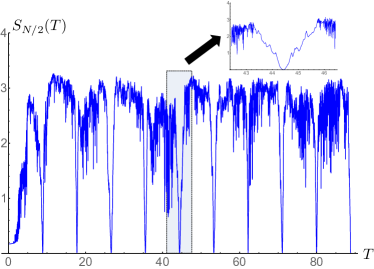
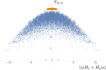
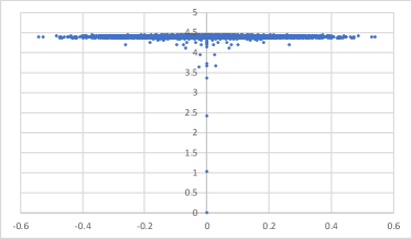
As an indicator of a nonthermal (or thermal) state, we use the entanglement entropy , where is the reduced density matrix obtained by taking the partial trace with respect to the sites . Thermal states have a large amount of the entanglement entropy, which are linearly dependent on the system size Page (1993); D’Alessio et al. (2016); Nakagawa et al. (2018); Lu and Grover (2019). If the entanglement entropy is small and independent of , the state is an nonthermal state. Now, let us discuss the entanglement entropy as a function of the period . We numerically calculate the entanglement entropies for all Floquet eigenstates. We use the open boundary condition with the system sizes and . Fig. 1 shows the -dependence of the minimum value of the entanglement entropies among all the eigenstates; interestingly, a resonance-like phenomenon is observed. The inset shows a magnified plot around , where almost vanishing entanglement entropy is observed, indicating a scar state. An important question is whether this is the state intrinsic to the Floquet operator or simultaneous eigenstate of the static Hamiltonian. To address this question, we consider the entanglement entropies for all Floquet eigenstates at a fixed period , and compare them with the entanglement entropies for the eigenstates of . If the Floquet scars are the simultaneous eigenstates for , one will see the coincidence of entanglement entropies between them. In Fig. 2, we present them as a function of the expectation value of for each eigenvalue. In the figure, the orange dots and the blue points represent the results for Floquet eigenstates and eigenstates of , respectively. Almost all Floquet eigenstates are thermal, as indicated by large values of entanglement entropies. The values are close to the theoretical value estimated from the reduced density matrix with an infinite temperature, i.e., 444 where is the number of Hilbert space for the size . The subtracted term 1/2 always appears in a finite-size system Page (1993). . Remarkably, exceptions for four states are seen, which have zero entanglement entropies (two states are degenerated at energy , and only three points are thus visible in the figure); however, all eigenstates of have finite entanglement entropies. Thus, the Floquet scars observed here are not simultaneous eigenstates of the static Hamiltonian, which are the desired FMS.
Exact description of the FMS.— We make the above numerical indication rigorous in the following, by providing an explicit description of the many-body scar state. We eventually show the following form for the FMS for the period with a positive integer :
| (7) |
where we obtain four FMSs for , and the detailed expressions of and are given below. Even at this level, we can list several physically crucial aspects. First, the period in the inset of Fig. 2 is consistent with the value (i.e., ). Second, the entanglement entropy is exactly zero from the structure of the above-mentioned expression. Third, the above expressions are different from the Lin-Motrunich (LM) eigenstates for the static Hamiltonian Lin and Motrunich (2019). The LM eigenstate is given with the matrix product form, which is clearly different from the above form. As explained below, the definition of the FMSs is that they are not the eigenstates of , but the simultaneous eigenstates for the unitary operations and .
We now consider the detailed expression for (7). Although the LM eigenstates are not identical to the FMS, those are still beneficial in deriving the FMSs. We first focus on the left part that consists of the sites from to . We note that the and are commutable to each other. When we fix the state at to the down state, can be regarded as the PXP model of the system size with the open boundary condition. In this case, the LM eigenstates are given by the following matrix product form:
| (8) |
where and
| (9) | ||||
| (10) |
The eigenenergies are E=0 for and for .
In addition, we make a new wave function by a linear transformation:
| (11) |
Through straightforward calculation, this state turns out to be identical to the following expression
| (12) |
where
| (13) |
with the new vector . It should be noted that the state (11) is a superposition of the two eigenstates with the energy and , and is therefore not the eigenstate of the Hamiltonian . However, when we consider the unitary time evolution starting from this state, the wave function returns to the initial state with the time , i.e., the two states are the eigenstates of .
A similar analysis is performed for the unitary time-evolution by considering the site to . Starting with fixing the state at the site to the down state, we eventually arrive at the following wave function:
| (14) |
where , and the function is given by
| (15) |
with the vector . The states (14) are the eigenstates for .
Crucially, both and contain the product states with the down states at the site and , and thus, we can safely merge these states to obtain the desired expression (7). From these derivations, one can see that our FMSs are not the eigenstates of the static Hamiltonian , but they are the simultaneous eigenstates for unitary operators and . The rigorous proof of the FMS by showing the explicit Floquet eigenstate, and the underlying physical mechanism, are the main results in this paper.
Periodic boundary condition and the Floquet-scar-engineering.—
In the case of the periodic boundary condition with the period , one can readily obtain the FMS by following a similar procedure as above. In this case, we have only one scar state, which is given by
| (16) |
where is a pure state defined from the site to :
| (17) |
The entanglement entropy for the subsystem consisting of the sites is exactly zero from the structure.
Having understood the underlying mechanism to have scar states, we now demonstrate that other systems which have scar states can be systematically engineered. We emphasize that many systems can be systematically constructed. We show an example of such applications below.
We consider the system of size , where and are integers. Then, we make a unitary time-evolution of each sites by dividing the Hamiltonian as follows:
| (18) | ||||
| (19) |
where and we impose the periodic boundary condition or the open one. By following the same procedure as before, regardless of the boundary conditions one can find the exact scar state for the period :
| (20) |
In this FMS, and appear alternatively. We note that the spins at the edges and are both down states for the open boundary condition. In (7) four FMS states do not have the down states at the edge. However, by superposing them we have the FMS which has and . In the same way we make the edge state in (20) the down states.
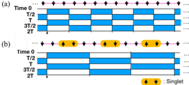
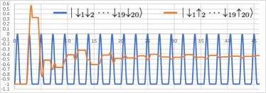
In Fig. 3a and b, two simplest cases of the protocol (18), (19), and the FMS state (20) are schematically illustrated. The upper figure in the inset is the case for and the lower one is for . Interestingly, (20) reduces to simple states; For , it is an all-down state, because the term vanishes. For , reduces to the singlet state. We note that for (20) becomes the FMS for with positive integer , because (20) is the superposition of and , whose eigenenergies are . This is twice as frequent as the periods for , because (20) for is the superposition of , and , whose eigenenergies are , , 0 and 0, respectively. The detailed explanation is provided in the Supplementary materials. The advantage of the FMS is clearly observed in time evolution. In Fig. 4, numerical results of the time evolution starting from the FMS (blue) and from the state (orange) are shown. We impose the open boundary condition and take in our numerical calculation. Starting with the FMS we see perfect revival to the initial state, while the spin decays quickly for the state. The value of after the relaxation is around , which is the ensemble average value at infinite temperature. We note that this is nonzero due to the Rydberg blockade.
Summary and perspective.— In this paper, we discussed the Floquet many-body scar states. We first classified the possible scar states into two classes. In the first class, the scar state is the simultaneous eigenstate for the Hamiltonian for any . This type is given by using the frustration-free Hamiltonian, such as the AKLT Hamiltonian. We focus on the second class, which has the scar state intrinsic to the Floquet operator (FMS). Our model consists of the PXP-type interactions without disorder. We exactly demonstrate that the FMSs certainly exist, by showing the explicit expressions of the eigenstates. The crucial mechanism of the FMSs discovered here is that the states are simultaneous eigenstates of different unitary operators, while they are not simultaneous eigenstates for the Hamiltonians. Another important feature is the absence of the conserved quantities in our system. Hence the mechanism presented in this paper should be different from those in the previous works where the system has conserved quantities Haldar et al. (2019). All the Hamiltonians in this study can be implemented in a chain of Rydberg dressed alkali-metal atoms in principle Bernien et al. (2017); Potirniche et al. (2017); Graham et al. (2019). In particular, the protocols depicted in Fig. 3 are the most feasible for experimental realization, because the FMS states reduce to simple states which can be readily prepared in experiments. It is an important future subject to observe the FMS in cold atoms experiments.
acknowledgments.— The authors thank W. W. Ho, H. Levine, and H. Katsura for useful discussions and valuable comments. S.S was supported by JSPS Overseas Research Fellowships (201860254). T.K. was supported by the RIKEN Center for AIP and JSPS KAKENHI Grant No. 18K13475. K.S. was supported by JSPS Grants-in-Aid for Scientific Research (JP16H02211).
References
- Popescu et al. (2006) S. Popescu, A. J. Short, and A. Winter, Nat Phys 2, 754 (2006).
- Goldstein et al. (2006) S. Goldstein, J. L. Lebowitz, R. Tumulka, and N. Zanghì, Phys. Rev. Lett. 96, 050403 (2006).
- Goold et al. (2016) J. Goold, M. Huber, A. Riera, L. del Rio, and P. Skrzypczyk, Journal of Physics A: Mathematical and Theoretical 49, 143001 (2016).
- Yukalov (2011) V. Yukalov, Laser Physics Letters 8, 485 (2011).
- Nandkishore and Huse (2015) R. Nandkishore and D. A. Huse, Annual Review of Condensed Matter Physics 6, 15 (2015), https://doi.org/10.1146/annurev-conmatphys-031214-014726 .
- D’Alessio et al. (2016) L. D’Alessio, Y. Kafri, A. Polkovnikov, and M. Rigol, Advances in Physics 65, 239 (2016), https://doi.org/10.1080/00018732.2016.1198134 .
- Gogolin and Eisert (2016) C. Gogolin and J. Eisert, Reports on Progress in Physics 79, 056001 (2016).
- Mori et al. (2018) T. Mori, T. N. Ikeda, E. Kaminishi, and M. Ueda, Journal of Physics B: Atomic, Molecular and Optical Physics 51, 112001 (2018).
- Reimann (2015) P. Reimann, New Journal of Physics 17, 055025 (2015).
- Deutsch (2018) J. M. Deutsch, Reports on Progress in Physics 81, 082001 (2018).
- Deutsch (1991) J. M. Deutsch, Phys. Rev. A 43, 2046 (1991).
- Srednicki (1994) M. Srednicki, Phys. Rev. E 50, 888 (1994).
- D’Alessio and Polkovnikov (2013) L. D’Alessio and A. Polkovnikov, Annals of Physics 333, 19 (2013).
- D’Alessio and Rigol (2014) L. D’Alessio and M. Rigol, Phys. Rev. X 4, 041048 (2014).
- Lazarides et al. (2014) A. Lazarides, A. Das, and R. Moessner, Phys. Rev. E 90, 012110 (2014).
- Kuwahara et al. (2016) T. Kuwahara, T. Mori, and K. Saito, Annals of Physics 367, 96 (2016).
- Mori et al. (2016) T. Mori, T. Kuwahara, and K. Saito, Phys. Rev. Lett. 116, 120401 (2016).
- Kim et al. (2014) H. Kim, T. N. Ikeda, and D. A. Huse, Phys. Rev. E 90, 052105 (2014).
- Mondaini et al. (2016) R. Mondaini, K. R. Fratus, M. Srednicki, and M. Rigol, Phys. Rev. E 93, 032104 (2016).
- Mondaini and Rigol (2017) R. Mondaini and M. Rigol, Phys. Rev. E 96, 012157 (2017).
- Haldar et al. (2019) A. Haldar, D. Sen, R. Moessner, and A. Das, arXiv , 1909.04064 (2019).
- Ponte et al. (2015a) P. Ponte, Z. Papić, F. m. c. Huveneers, and D. A. Abanin, Phys. Rev. Lett. 114, 140401 (2015a).
- Ponte et al. (2015b) P. Ponte, A. Chandran, Z. Papić, and D. A. Abanin, Annals of Physics 353, 196 (2015b).
- Turner et al. (2018a) C. J. Turner, A. A. Michailidis, D. A. Abanin, M. Serbyn, and Z. Papić, Nature Physics 14, 745 (2018a).
- Turner et al. (2018b) C. J. Turner, A. A. Michailidis, D. A. Abanin, M. Serbyn, and Z. Papić, Phys. Rev. B 98, 155134 (2018b).
- Moudgalya et al. (2018) S. Moudgalya, S. Rachel, B. A. Bernevig, and N. Regnault, Phys. Rev. B 98, 235155 (2018).
- Ho et al. (2019) W. W. Ho, S. Choi, H. Pichler, and M. D. Lukin, Phys. Rev. Lett. 122, 040603 (2019).
- Khemani et al. (2019) V. Khemani, C. R. Laumann, and A. Chandran, Phys. Rev. B 99, 161101 (2019).
- James et al. (2019) A. J. A. James, R. M. Konik, and N. J. Robinson, Phys. Rev. Lett. 122, 130603 (2019).
- Choi et al. (2019) S. Choi, C. J. Turner, H. Pichler, W. W. Ho, A. A. Michailidis, Z. Papić, M. Serbyn, M. D. Lukin, and D. A. Abanin, Phys. Rev. Lett. 122, 220603 (2019).
- Bernien et al. (2017) H. Bernien, S. Schwartz, A. Keesling, H. Levine, A. Omran, H. Pichler, S. Choi, A. S. Zibrov, M. Endres, M. Greiner, V. Vuletić, and M. D. Lukin, Nature 551, 579 EP (2017).
- Lin and Motrunich (2019) C.-J. Lin and O. I. Motrunich, Phys. Rev. Lett. 122, 173401 (2019).
- Pai and Pretko (2019) S. Pai and M. Pretko, Phys. Rev. Lett. 123, 136401 (2019).
- Khemani and Nandkishore (2019) V. Khemani and R. Nandkishore, arXiv , 1904.04815 (2019).
- Nandkishore and Hermele (2019) R. M. Nandkishore and M. Hermele, Annual Review of Condensed Matter Physics, Annual Review of Condensed Matter Physics 10, 295 (2019).
- Pai et al. (2019) S. Pai, M. Pretko, and R. M. Nandkishore, Phys. Rev. X 9, 021003 (2019).
- Potirniche et al. (2017) I.-D. Potirniche, A. C. Potter, M. Schleier-Smith, A. Vishwanath, and N. Y. Yao, Phys. Rev. Lett. 119, 123601 (2017).
- Note (1) When has symmetries and corresponding conserved quantities, we divide the Hilbert space into the sectors of the conserved quantities and look into one of the sectors which have exponentially large dimension.
- Note (2) This class of the Floquet scar can be easily demonstrated when we employ the frustration-free Hamiltonian, where the ground state is a simultaneous eigenstate of all local interaction terms. For instance, we can consider the decomposition of the AKLT Hamiltonian. Let be which is the interaction term between the sites and , where is a spin-1 operator. Then for even size , we set and . Note that and are uncommutable to each other, and those are nonintegrable. Frustration-free leads to that the ground state for is also eigenstate of and .
- Affleck et al. (1987) I. Affleck, T. Kennedy, E. H. Lieb, and H. Tasaki, Phys. Rev. Lett. 59, 799 (1987).
-
Note (3)
In the open boundary condition, the original transverse
Ising model is given by
where and are imposed. We consider a constrained Hilbert space without any adjacent up states. When set , all eigenstates in this restricted Hilbert space are degenerate in their energies. Then, the transverse field term is treated by the perturbation to get the PXP model. From this picture, the decomposition of the Hamiltonians (5) and (6) can be derived by applying the time-dependent transverse field. Namely, we define and , then we apply time-dependent fields as for , and for . - Schauß et al. (2015) P. Schauß, J. Zeiher, T. Fukuhara, S. Hild, M. Cheneau, T. Macrì, T. Pohl, I. Bloch, and C. Gross, Science 347, 1455 (2015).
- Labuhn et al. (2016) H. Labuhn, D. Barredo, S. Ravets, S. de Léséleuc, T. Macrì, T. Lahaye, and A. Browaeys, Nature 534, 667 EP (2016).
- Graham et al. (2019) T. M. Graham, M. Kwon, B. Grinkemeyer, Z. Marra, X. Jiang, M. T. Lichtman, Y. Sun, M. Ebert, and M. Saffman, arXiv , 1908.06103 (2019).
- Page (1993) D. N. Page, Phys. Rev. Lett. 71, 1291 (1993).
- Nakagawa et al. (2018) Y. O. Nakagawa, M. Watanabe, H. Fujita, and S. Sugiura, Nature Communications 9, 1635 (2018).
- Lu and Grover (2019) T.-C. Lu and T. Grover, Phys. Rev. E 99, 032111 (2019).
- Note (4) where is the number of Hilbert space for the size . The subtracted term 1/2 always appears in a finite-size system Page (1993).
Appendix A Two-sites protocol
We show the results of the system where two consecutive sites are periodically driven. The two sites protocol is schematically shown in Fig. 3 in the main text . We show that the FMSs are stabler than other states under the time evolution of this protocol. Also, we find that the two sites protocol is a somewhat special case which has more FMSs than other protocols in our paper have. The results are summarized as follows. As explained in the main part, the all-down state is a FMS of certain periods, where is an arbitrary integer number. However, this is not the only FMS in the two sites protocol. We find that there are exponentially-large number of other FMSs. We also show that FMSs exist in other periods.
A.1 Four-sites system
In order to explicitly see the time evolution of each period, we consider the minimum model of four sites:
| (21) |
where the Rabi oscillation is induced on site 2 and 3. The eigenenergies and eigenstates are given by
| (22) | |||
| (23) | |||
| (24) | |||
| (25) | |||
| (26) | |||
| (27) | |||
| (28) | |||
| (29) |
where numbers of the states are the energy eigenvalues and the subscripts are the indices of degenerated states, e.g., and are two eigenstates of zero energy eigenvalue.
We consider the unitary time evolution given by
| (30) |
and where is an integer. The states (22)-(25) do not acquire any phase after the time evolution (30), while the others (26)-(29) do. Therefore, consider a superposition of the states (22)-(25)
| (31) |
where are any complex number. does not experience dephasing under :
| (32) |
works as an identity operator for . Similarly, for where in an integer (24) and (25) acquire the same phase. Hence, any superposition of them are conserved by (30).
A.2 FMS at
Given this mechanism of the minimum model, we can readily construct FMSs in the two sites protocol shown in Fig. 3 in the main text. Two Hamiltonians are applied to the system alternatively:
| (33) | ||||
| (34) |
where and we impose the periodic boundary condition. When a quantum state is the product of the simultaneous eigenstate of (33) and (34), it is a FMS. One solution exists at where is an integer number. With this period, any superposition of (24) and (25) returns to the same state after the time evolution in the Four sites system; is such a state because . Since a longer chain described by (33) and (34) consists of the four-sites system, is a FMS for this protocol:
| (35) |
In Fig. 5, we show the distribution of the entanglement entropy for . We see a scar state at , while other states are distributed around 4.4, which is estimated from the density matrix at infinite temperature. At , we also find several states which have small . They are FMSs, e.g., for N=20 we can readily show that
| (36) |
is a FMS whose Floquet eigenvalue is , where we introduce notations
| (37) | |||
| (38) | |||
| (39) |
The time evolution of the all-down state in this protocol is shown in Fig. 3 in the main text. We see the persistent oscillation in the whole periods as is expected for the FMS. By contrast, the spin decays rapidly in state in Fig. 3 in the main text.
A.3 Another FMS at
A.4 Exponentially many FMSs at
When for being an integer, the all-down state is again the eigenstate of the Floquet operator, (35). We show that exponentially large number of the Floquet eigenstate violate the Floquet ETH.
Returning to the four-sites system, by superposing the states (22)-(25) we can make four product states, . Hence, if a product state is either of these four states for all , this state is a FMS. More precisely, we can show that the configuration is always conserved by , because we cannot flip the left edge state and the right edge state . Hence, product states in which and appear alternatively become the eigenstate of . For example,
| (40) | |||
| (41) |
satisfy this condition. Since the number of such FMSs can be counted in a similar manner to how we count the dimension of PXP model, the number of the FMSs is an exponential of .
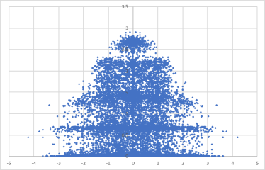
In Fig. 6, the entanglement entropy of all the Floquet eigenstates in this model is shown. Exponentially large number of the Floquet eigenstate are located on the horizontal axis. They are the FMSs such as (40) and (41). However, we also see many other Floquet eigenstates have lower entanglement entropy, e.g., large number of them are concentrated around .