TOI-677 b: A Warm Jupiter (P=11.2d) on an eccentric orbit transiting a late F-type star

Abstract

We report the discovery of TOI-677 b, first identified as a candidate in light curves obtained within Sectors 9 and 10 of the Transiting Exoplanet Survey Satellite (TESS) mission and confirmed with radial velocities. TOI-677 b has a mass of ${\rm M_{p}}$= $1.236_{-0.067}^{+0.069}$ ${\rm M_{J}}$, a radius of ${\rm R_{P}}$= $1.170\pm 0.03$ ${\rm R_{J}}$, and orbits its bright host star ($V=9.8$ mag) with an orbital period of $11.23660\pm 0.00011$ d, on an eccentric orbit with $e=0.435\pm 0.024$. The host star has a mass of ${\rm M}_{\star}$= $1.181\pm 0.058$ ${\rm M}_{\odot}$, a radius of ${\rm R}_{\star}$= $1.28_{-0.03}^{+0.03}$ ${\rm R}_{\odot}$, an age of $2.92_{-0.73}^{+0.80}$ Gyr and solar metallicity, properties consistent with a main sequence late F star with $T_{\rm eff}=6295\pm 77$ K. We find evidence in the radial velocity measurements of a secondary long term signal which could be due to an outer companion. The TOI-677 b system is a well suited target for Rossiter-Mclaughlin observations that can constrain migration mechanisms of close-in giant planets.

1 Introduction

In the past two decades the population of known transiting exoplanets has grown at an accelerating pace. While the Kepler satellite (Borucki et al., 2010) dominates the overall number of discoveries, the particular class of close-in gas giants around nearby stars were until recently most efficiently discovered by wide-field photometric series (e.g. Bakos et al., 2004; Pollacco et al., 2006; Pepper et al., 2007; Bakos et al., 2013; Talens et al., 2017). Due to the biases inherent to ground based observatories, most of the discoveries of these surveys have periods $P\lesssim 10$d. Systems of stations around the globe such as the HATSouth survey can in principle improve the efficiency of discovery for longer periods, but the number of systems with $P>10$d uncovered by wide-field ground-based surveys is small, with the current record holder being HATS-17b with $P\approx 16$d (Brahm et al., 2016).

The population of close-orbiting gas giants has opened a number of questions about their physical structural and dynamical evolution which are still topics of active research (Dawson & Johnson, 2018). In particular, the nature of the migration history and the detailed mechanism of radius inflation for hot Jupiters need further elucidation. In order to make further progress on those fronts the population of warm giants, loosely defined as systems with periods $P\gtrsim 10$d, is of importance. They are close enough to the star that they are likely to have undergone significant migration, but not as close that tidal effects can erase the potential imprints of that migration (Albrecht et al., 2012; Dawson, 2014; Li & Winn, 2016). In the same vein, they are far enough from their parent star that their radii have not been inflated by the mechanism that acts to bloat the radii of hotter giants (Kovács et al., 2010; Demory & Seager, 2011; Miller & Fortney, 2011). But while it is clear that these systems are very interesting, the population of known warm giants around nearby stars (allowing the most detailed characterization) is still very small. The launch of the TESS mission (Ricker et al., 2015) is changing that. By scanning nearby stars around the whole sky the expectation is that hundreds of giant planets with $P\gtrsim 10$ d will be uncovered (Sullivan et al., 2015; Barclay et al., 2018).

In this work we present the discovery originating from a TESS light curve of an eccentric warm giant planet with a period of $P=11.23660\pm 0.00011$ days orbiting a bright late F star. This is part of a systematic effort to characterize warm giants in the southern hemisphere uncovered with TESS which has contributed to the discovery and mass measurement of three warm giants already (Brahm et al., 2019; Huber et al., 2019; Rodriguez et al., 2019). The paper is structured as follows. In § 2 we describe the observational material which gets used to perform a global modeling of the system as described in § 3. The results are then discussed in § 4.

2 Observations

2.1 TESS

Between 2019 March 01 and 2019 April 22, the TESS mission observed TOI-677 (TIC 280206394, 2MASS J09362869-5027478, TYC 8176-02431-1, WISE J093628.65-502747.3) during the monitoring of Sectors 9 and 10, using camera 3 and CCDs 1 and 2, respectively. The TESS Science Processing Operations Center (SPOC; for an overview of the processing it carries out see Jenkins et al., 2016) Transiting Planet Search module detected the planetary signature in the Sector 9 processing run and in the Sectors 1-13 multi-sector search and triggered the Data Validation module (Twicken et al., 2018; Li et al., 2019) to analyze the transit-like feature in the Sector 9 and combined Sectors 9 and 10 light curves. All diagnostics tests performed as part of the data validation report, including the odd/even depth test, the signal to noise ratio, the impact parameter, the statistical bootstrap probability, the ghost diagnostic, and the difference image centroid offset from the TIC position and from the out-of-transit centroid, strongly favored the planetary hypothesis and resulted in the promotion of TOI-677 to the list of targets of interest.

The properties of TOI-677 as obtained from literature sources and derived in this work are detailed in Table 1. The target was observed in short (2 min) cadence, and we downloaded the PDC (Pre-search Data Conditioning) SAP light curves from the Mikulski Archives for Space Telescopes. The PDC SAP light curves have systematic trends removed by the use of co-trending basis vectors (Smith et al., 2012; Stumpe et al., 2014), and are produced by the TESS SPOC at NASA Ames Research Center. We masked the regions of high scattered light as indicated in the data release notes for each of the sectors, augmenting the masked windows in a few cases where it was evident that there were some remaining trends that were insufficiently masked. We did not mask datapoints with data quality flags, as we noticed that all of the second transit had been masked with a flag value of 2048 (stray light from Earth or Moon in camera field of view), but inspection of the masked portions revealed no anomalous signs on the light curve.

Figure 1: The 2 min cadence TESS light curve. These are the PDC SAP measurements produced by the SPOC pipeline. Four transits are clearly seen in the TESS photometry, with the middle transit falling within a gap.

The TESS light curve is shown in Figure 1, where four transits are clearly seen. The out-of-transit light curve is remarkably flat. We estimated the power spectral density of the out-of-transit light curve of TOI-677 using the method of Welch (1967) as implemented in the scipy.signal Python module and found it to be featureless and at precisely the level expected given the reported photometric uncertainties of the magnitude measurements (see Figure 2). We conclude from this exercise that there is no need for any deterministic or stochastic component beyond the white noise implied by the photometric uncertainties in the modeling of the out-of-transit light curve. Because of this we only fit for regions of $\approx$ 1d around each transit, removing the median value calculated in the out-of-transit portion for each transit. The TESS data used for the analysis is presented in Table 3

Figure 2: Power spectral density of the out-of-transit TESS light curve. The dashed line marks the expected value of the power spectral density, estimated as $\langle\sigma_{i}^{2}\rangle/(\nu_{u}-\nu_{l})$, where $\langle\sigma_{i}^{2}\rangle$ is the average measurement variance of the TESS photometry, $\nu_{l}=0$ and $\nu_{u}\approx 0.004$ Hz is the Nyquist frequency for the short cadence sampling.

2.2 Spectroscopy

We followed up TOI-677 with several spectrographs in order to confirm the TESS transiting planet candidate and to measure its mass. In what follows we describe the observations obtained by each spectrograph we used. The derived radial velocities, and bisector span measurements when available, are reported in Table 4.

2.2.1 FEROS

TOI-677 was monitored with the FEROS spectrograph (R$\approx$48000, Kaufer et al., 1999) mounted at the MPG 2.2m telescope at La Silla Observatory between May and July of 2019, where 26 spectra were obtained. Observations were performed in simultaneous calibration mode, with the secondary fibre observing a thorium-argon (ThAr) lamp to trace the instrumental variations produced by changes in the environment during the science exposures. The adopted exposure times were of 300 s and 400 s, which translated into a signal-to-noise ratio ranging between 40 and 150 per resolution element. The FEROS data were processed with the CERES pipeline (Brahm et al., 2017a), which delivers the radial velocities corrected by the instrumental drift variations and the by the Earth’s motion. These radial velocities were obtained with the cross-correlation technique, where a G2-type binary mask was used as template. From this cross-correlation peak CERES also computes the bisector span measurements, and delivers a rough estimate of the stellar parameters by comparing the continuum normalized spectrum with a grid of synthetic ones.

2.2.2 Coralie

We monitored TOI-677 with the Coralie spectrograph (R$\approx$60000, Mayor et al., 2003) mounted on the Swiss-Euler 1.2m telescope in six different epochs. These observations were also performed with the simultaneous calibration technique, but in this case the secondary fibre is illuminated by a Fabry-Perot etalon. We adopted an exposure time of 300 s, which produced spectra having a typical signal-to-noise ratio of 30 per resolution element. Coralie data were also processed with the CERES pipeline for obtaining the radial velocities.

2.2.3 CHIRON

We collected a total of 11 spectra of TOI-677 using the CHIRON high-resolution spectrograph (Tokovinin et al., 2013), between May 17 and June 19, 2019. The exposure time was between 750–1200 s, leading to a signal-to-noise ratio (SNR) per pixel between $\approx$ 20 - 35. CHIRON is mounted on the SMARTS 1.5 m telescope at the Cerro Tololo Inter-American observatory in Chile, and is fed by an octagonal multi-mode optical fibre. For these observations we used the image slicer, which delivers relatively high throughput and high spectral resolution (R $\approx$ 80,000). The radial velocities were computed from the cross-correlation function between the individual spectra and a high-resolution template of the star, which is built by stacking all individual observations of this star. Since CHIRON is not equipped with a simultaneous calibration, we observed the spectrum of a Th-Ar lamp before the science observations, to correct for the instrumental drift. Using this method we have measured a long-term RV stability of $<$ 10 m s^-1 on bright targets (t${}_{exp}<$ 60 s) and $<$ 15 m s^-1 for fainter objects (t${}_{exp}<$ 1800 s). For more details of the method see Wang et al. (2019) and Jones et al. (2019).

2.2.4 NRES

NRES (Siverd et al., 2018) is a global array of echelle spectrographs mounted on 1-meter telescopes, with a resolving power of $\approx$ 53,000. TOI-677 was observed at 12 epochs with the NRES node located at the Cerro Tololo Inter-American Observatory. At each observing epoch, three consecutive 1200 s exposures were obtained, with individual signal-to-noise ratio $\gtrsim$40. The velocity of each exposure was derived via cross-correlation with a PHOENIX template (Husser et al., 2013) with $T_{\rm eff}$=5800 K, $\log{g}$=3.5, ${\rm[Fe/H]}$=-0.5 and $v\sin{i}$=7 km/s. Systematic drifts were corrected per order (e.g., Engel et al., 2017) and the radial velocity of each epoch was then taken as the mean of the three exposures.

2.2.5 Minerva-Australis

We obtained 17 observations on nine separate nights with the MINERVA-Australis telescope array (Addison et al., 2019) at Mount Kent Observatory in Queensland, Australia. All of the telescopes in the MINERVA-Australis array simultaneously feed a single Kiwispec R4-100 high-resolution (R$\approx$80,000) spectrograph with wavelength coverage from 500 to 630 nm over 26 echelle orders. We derived radial velocities for each telescope using the least-squares analysis of Anglada-Escudé & Butler (2012) and corrected for spectrograph drifts with simultaneous Thorium-Argon arc lamp observations. TOI-677 was observed with telescopes 3, 4 and 5 of the array, the derived radial velocities are reported under the instrument labels Minerva_T3, Minerva_T4 and Miverva_T5 in Table 4.

2.3 Ground-based photometry

2.3.1 Shared Skies Telescope at Mt. Kent Observatory (SSMKO)

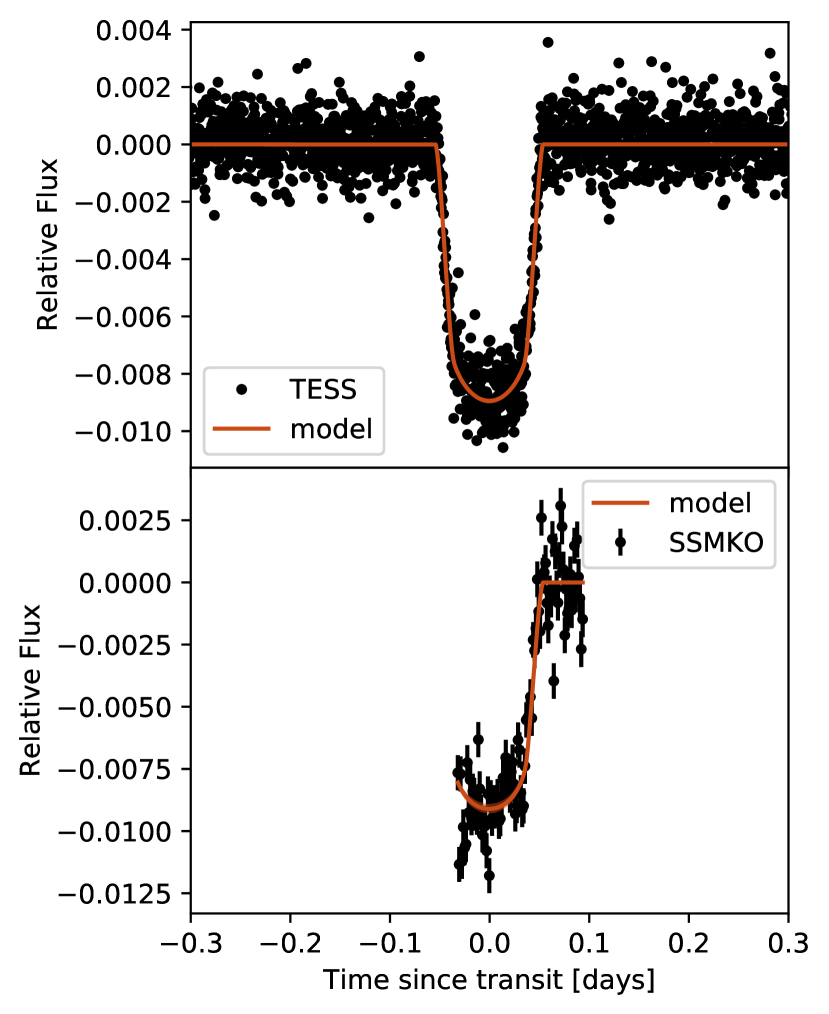
Figure 3: Photometric data with the trend subtracted as a function of phase for the two photometric instruments used in this work (TESS, SSMKO). The orange line shows the posterior transit model.

TOI-677 was observed on the night of UTC 2019-05-09 with the University of Louisville’s Shared Skies MKO-CDK700 (SSMKO) telescope at Mt. Kent Observatory of the University of Southern Queensland, Australia. The telescope is a 0.7-meter corrected Dall-Kirkham with a Nasmyth focus manufactured by Planewave. Images with an exposure time of 64 s were taken through a Sloan i’ filter using an Apogee U16 CCD camera with a Kodak KAF-16801E sensor. A sequence of 92 images were acquired over 180 minutes. The light curve, which is shown in Figure 3 displays a clear egress. No significant activity or modulation other than the transit itself was apparent in the light curve, which shows residuals of 0.85 ppt at the observational cadence. The SSMKO data used for the analysis is presented in Table 3

2.4 Gaia DR2

Observations of TOI-677 by Gaia were reported in DR2 (Gaia Collaboration et al., 2016, 2018). From GAIA DR2, TOI-677 has a parallax of $7.02\pm 0.03$ mas, an effective temperature of $T_{\rm eff}=5895_{-200}^{+105}$ K and a radius of ${\rm R}_{\star}=1.37_{-0.05}^{+0.1}\,\,{\rm R}_{\odot}$. The parallax obtained from GAIA was used to determine the stellar physical parameters of TOI-677 as described in Section 3.1. In our analysis we corrected the GAIA DR2 parallax for the systematic offset of -82 $\mu$as reported in Stassun & Torres (2018).

2.5 High spatial resolution imaging

The relatively large angle subtended by the TESS pixels, approximately 21″ on a side, leave it susceptible to photometric contamination from nearby stars, including additional wide stellar companions. We searched for nearby sources to TIC 280206394 with SOAR speckle imaging (Tokovinin, 2018) on 18 May 2019 UT, observing through a similar visible bandpass as TESS. More details of these observations are available in Ziegler et al. (2019). We detected no nearby sources within 3″ of TIC 280206394. The 5$\sigma$ detection sensitivity and the speckle auto-correlation function from the SOAR observation are plotted in Figure 4.

Figure 4: The $I$-band auto-correlation function from Speckle using SOAR. The 5-$\sigma$ contrast curve for TOI-677 is shown by the black points. The black solid line is the linear fit to the data for separations $<0\farcs 2$ and $>0\farcs 2$. The auto-correlation function is shown within the contrast curve plot.

The radial velocity variations measured on TOI-677 phase with the transit signal. This fact, combined with the lack of nearby companions, the lack of correlation of the bisector span measurements with orbital phase and the tests carried out as part of the SPOC data validation report show that the transit is not caused by a blended stellar eclipsing binary.

3 Analysis

3.1 Stellar parameters

In order to characterize the star, we follow the same procedure presented in Brahm et al. (2019). First, we compute the stellar atmospheric parameters using the co-added FEROS spectra through the ZASPE code (Brahm et al., 2017b). ZASPE estimates $T_{\rm eff}$, $\log{g}$, ${\rm[Fe/H]}$, and $v\sin{i}$, by comparing an observed spectrum with a grid of synthetic models generated with the ATLAS9 atmospheres (Castelli & Kurucz, 2004).

Then, we estimate the physical parameters of the host star using the publicly available broadband photometry of GAIA (G, B_P, R_P) and 2MASS (J, H, K_S), which is compared to the synthetic magnitudes provided by the PARSEC stellar evolutionary models by using the distance to the star from the Gaia DR2 parallax. For a given stellar mass, age and metallicity, the PARSEC models can deliver a set of synthetic absolute magnitudes and other stellar properties (e.g. stellar luminosity, effective temperature, stellar radius).

We determine the posterior distributions for ${\rm M}_{\star}$, Age, and A_V, via an MCMC code using the emcee package (Foreman-Mackey et al., 2013), where we fix the metallicity of the PARSEC models to that obtained with ZASPE, and we apply the Cardelli et al. (1989) extinction laws to the synthetic magnitudes.

This procedure provides a more precise estimation of $\log{g}$  than the one obtained from the spectroscopic analysis. For this reason we iterate the procedure where we fix the $\log{g}$ value when running ZASPE to the value obtained from the PARSEC models. The resulting values are $T_{\rm eff}=6295\pm 77$ K, ${\rm[Fe/H]}=0.00\pm 0.05$ dex, $\log{g}=4.291\pm 0.025$, $v\sin{i}=7.80\pm 0.19$ ${\rm km\,s^{-1}}$, $A_{V}=0.226_{-0.058}^{+0.056}$ mag, age $=2.92_{-0.73}^{+0.80}$ Gyr, $L_{\star}=2.33\pm 0.11$ ${\rm L}_{\odot}$  ${\rm M}_{\star}=1.170\pm 0.06$ ${\rm M}_{\odot}$ and ${\rm R}_{\star}=1.282\pm 0.03$ ${\rm R}_{\odot}$. The values and uncertainties of ${\rm M}_{\star}$ and ${\rm R}_{\star}$ are used to define priors for them in the global analysis described in the next section.

Table 1: Stellar properties of TOI-677 

Parameter	Value	Reference
Names	TIC 280206394	TIC
	2MASS J09362869-5027478	2MASS
	TYC 8176-02431-1	TYCHO
	WISE J093628.65-502747.3	WISE
RA (J2000)	15h32m17.84s
DEC (J2000)	-22d21m29.74s
$\mu_{\alpha}$ (mas yr-1)	-24.82 $\pm$ 0.05	Gaia
$\mu_{\delta}$ (mas yr-1)	42.42 $\pm$ 0.05	Gaia
$\pi$ (mas)	$7.02\pm 0.03$	Gaia
TESS (mag)	9.24 $\pm$ 0.018	TIC
G (mag)	9.661 $\pm$ 0.020	Gaia
BP (mag)	9.968 $\pm$ 0.005	Gaia
RP (mag)	9.229 $\pm$ 0.003	Gaia
J (mag)	8.722 $\pm$ 0.020	2MASS
H (mag)	8.470 $\pm$ 0.038	2MASS
Ks (mag)	8.429 $\pm$ 0.023	2MASS
$T_{\rm eff}$(K)	$6295\pm 77$	zaspe
$\log{g}$(dex)	$4.291\pm 0.025$	zaspe
${\rm[Fe/H]}$(dex)	$0.00\pm 0.05$	zaspe
$v\sin{i}$(km s-1)	$7.80\pm 0.19$	zaspe
${\rm M}_{\star}$(${\rm M}_{\odot}$)	$1.181\pm 0.058$	this work
${\rm R}_{\star}$(${\rm R}_{\odot}$)	$1.28_{-0.03}^{+0.03}$	this work
Age (Gyr)	$2.92_{-0.73}^{+0.80}$	this work
$\rho_{*}$(g cm-3)	$0.80_{-0.06}^{+0.06}$	this work

3.2 Global modeling

We performed joint modelling of the radial velocity and photometric data using the exoplanet toolkit (Foreman-Mackey et al., 2019). The radial velocities used are given in Table 4 and the photometric data are given in Table 3. We denote the TESS photometric time series by $\{y_{T}(t_{i})\}_{i=1}^{n_{T}}$, the SSMKO one by $\{y_{S}(t_{i})\}_{i=1}^{n_{S}}$, and the radial velocity measurements (with their mean values removed) by $\{y_{\rm F}(t_{i})\}_{i=1}^{n_{F}}$, $\{y_{\rm C}(t_{i})\}_{i=1}^{n_{C}}$, $\{y_{\rm\chi}(t_{i})\}_{i=1}^{n_{\chi}}$, $\{y_{\rm N}(t_{i})\}_{i=1}^{n_{N}}$ and $\{y_{\rm M(i)}(t_{i})\}_{i=1}^{n_{N}}$ for FEROS, Coralie, CHIRON, NRES, and Minerva Australis respectively. In the case of Minerva, $M(i)$ is a function that returns the telescope used at observation $t_{i}$ (recall the Minerva observations include three different telescopes). The observational uncertainties are denoted by $\sigma_{*}(t_{i})$, where $*$ can take the value of any of the instrument labels. As shown in § 2.1, the TESS light curve shows no evidence of additional structure beyond white noise. The TESS photometric time series is therefore modeled as

$$y_{T}(t_{i}) =\mathcal{T}(t_{i};\mathbf{p})+N(0,\sigma^{2}_{T,i}),$$ (1)

where $N(0,\sigma^{2})$ denotes a Normal distribution of mean 0 and variance $\sigma^{2}$, $\mathcal{T}(t_{i};\mathbf{p})$ is the transit model, and $\mathbf{p}$ is the vector of model parameters. Explicitly,

$$\mathbf{p} =(R_{p},b,P,t_{0},e,\omega,R_{*},M_{*},u_{1},u_{2}),$$ (2)

where $R_{p}$ is the planetary radius, $b$ is the impact parameter, $P$ is the period, $t_{0}$ the reference time of mid-transit, $e$ the eccentricity, $\omega$ the angle of periastron, $R_{*}$ and $M_{*}$ the stellar radius and mass, and $u_{1}$ and $u_{2}$ the limb-darkening law coefficients, which we describe using a quadratic law.

The SSMKO photometric time series is modeled as

$$y_{S}(t_{i}) =\mathcal{T}(t_{i};\mathbf{p_{u}})+N(0,\sigma^{2}_{S,i}+\eta_{S}^{2})$$

$$+b_{0}+b_{1}(t_{i}-t_{0})$$

$$\equiv\phi_{S}(t_{i})+N(0,\sigma^{2}_{S,i}),$$ (3)

where the $\{b_{i}\}$ coefficients accounts for up to a linear systematic trend in the photometry, $\sigma^{2}_{S,i}$ are the reported photometric uncertainties, and $\eta_{S}$ is an additional photometric variance parameter. The parameter vector is the same as that for TESS, but the limb darkening coefficients are fixed to the values $(u_{1},u_{2})=(0.2489,0.305)$. These values were calculated using the ATLAS atmospheric models and the Sloan i’ band using the limb darkening coefficient calculator (Espinoza & Jordán, 2015), and in particular using the methodology of sampling the limb darkening profile in 100 points as described in Espinoza & Jordán (2015). We chose to fix the limb darkening coefficients given that the SSMKO light curve covers only the egress. The radial velocity times series are modeled as

$$y_{*}(t_{i}) =\mathcal{O}(t_{i};\mathbf{q})+N(0,\sigma^{2}_{*,i}+\eta^{2}_{*})+\gamma_{*}$$

$$a_{0}+a_{1}(t-t_{0})$$

$$\equiv r_{*}(t_{i})+N(0,\sigma^{2}_{*,i}+\eta^{2}_{*})$$ (4)

where $\mathcal{O}$ represents the Keplerian radial velocity curve and the parameter vector of the model, a subset of $\mathbf{p},$ is $\mathbf{q}=(P,t_{0},e,\omega,M_{*})$. The wildcard $*$ can take the values ${F,C,\chi,N,M}$ for FEROS, Coralie, CHIRON, NRES and Minerva respectively, and $\eta^{2}_{*}$ is a white noise “jitter” terms to account for additional variance not accounted for in the observational uncertainties. The parameters ${a_{i}}$ account for up to a linear systematic trend in the radial velocities. We set priors for $\eta^{2}_{*}$ by first running a model without jitter terms, and determining for each instrument how much extra variance was present around the posterior model over that predicted by the observational uncertainties. We note that for NRES we found no need for a jitter term and thus we set $\eta_{N}\equiv 0$. The log-likelihood $l$ is given by

$$-2l(\mathbf{p}) =\medmath$$

$$\medmath{+\sum_{i=1}^{n_{S}}(\sigma_{S,i}^{2}+\eta_{S}^{2})^{-2}(y_{S,i}-\phi_{S,i})^{2}+\ln(\sigma_{S,i}^{2}+\eta_{S}^{2})}$$

$$\medmath{+\sum_{i=1}^{n_{F}}(\sigma_{F,i}^{2}+\eta^{2}_{F})^{-2}(y_{F,i}-r_{F,i})^{2}+\ln(\sigma_{F,i}^{2}+\eta^{2}_{F})}$$

$$\medmath{+\sum_{i=1}^{n_{C}}(\sigma_{C,i}^{2}+\eta_{C}^{2})^{-2}(y_{C,i}-r_{C,i})^{2}+\ln(\sigma_{C,i}^{2}+\eta_{C}^{2})}$$

$$\medmath{+\sum_{i=1}^{n_{\chi}}(\sigma_{\chi,i}^{2}+\eta^{2}_{\chi})^{-2}(y_{\chi,i}-r_{\chi,i})^{2}+\ln(\sigma_{\chi,i}^{2}+\eta^{2}_{\chi})}$$

$$\medmath{+\sum_{i=0}^{n_{M}}(\sigma_{M(i),i}^{2}+\eta^{2}_{M})^{-2}(y_{M,i}-r_{M(i),i})^{2}+\ln(\sigma_{M(i),i}^{2}+\eta^{2}_{M})}$$

$$\medmath{+\sum_{i=1}^{n_{N}}\sigma_{N,i}^{-2}(y_{N,i}-r_{N,i})^{2}}.$$ (5)

Posteriors were sampled using an Monte Carlo Markov Chain algorithm, specifically the No U-Turn Sampler (NUTS, Hoffman & Gelman, 2011) as implemented in the PyMC3 package through exoplanet. We sampled using 4 chains and 3000 draws, after a tuning run of 4500 draws where the step sizes are optimized. Convergence was verified using the Rubin-Gelman and Geweke statistics. The effective sample size for all parameters, as defined by (Gelman et al., 2013), was $>4000$. The priors are detailed in Table 2. Priors for $M_{*}$ and $R_{*}$ stem from the analysis described in § 3.1. The priors on $P$, $T_{0}$, $\ln({\rm M_{p}}/m{\rm M}_{\oplus})$, $e$, $\{a_{i}\}_{i=0}^{1}$ were obtained from a fit to the radial velocities alone carried out with the radvel package (Fulton et al., 2018).

Table 2: Prior and posterior parameters of the global fit. Derived parameters which are deterministic functions of the parameters fitted for are presented in the bottom part of the table. For the priors, $N(\mu,\sigma^{2})$ stands for a normal distribution with mean $\mu$ and variance $\sigma^{2}$, $N(\mu,\sigma^{2};l,u)$ is a bounded normal distribution with lower and upper limits given by $l$ and $u$, respectively, and $U(a,b)$ stands for a uniform distribution between $a$ and $b$.

Parameter	Prior	Value
P (days)	$N(11.27,0.7^{2})$	$11.23660\pm 0.00011$
T0 (BJD)	$N(2458547.4743,0.0012^{2})$	$2458547.47448_{-0.00029}^{+0.00028}$
$\ln({\rm M_{p}}/{\rm M}_{\oplus})$	$N(\ln(500),0.3^{2})$	$5.973_{-0.056}^{+0.054}$
${\rm R}_{\star}$ (${\rm R}_{\odot}$)	$N(1.282,0.03^{2})$	$1.28_{-0.03}^{+0.03}$
${\rm M}_{\star}$ (${\rm M}_{\odot}$)	$N(1.17,0.06^{2})$	$1.181\pm 0.058$
r1	$U(0,1)$	$0.0942_{-0.0012}^{+0.0010}$
r2	$U(0,1)$	$0.723_{-0.024}^{+0.018}$
u${}_{1}^{\rm TESS}$	$U(0,1)$	$0.50_{-0.27}^{+0.19}$
u${}_{2}^{\rm TESS}$	$U(0,1)$	$-0.06_{-0.23}^{+0.33}$
$e$	$N_{b}(0.4,0.1;0,1)$	$0.435\pm 0.024$
$\omega$ (rad)	$U(-\pi,\pi)$	$1.230_{-0.063}^{+0.063}$
$\gamma_{\rm FEROS}$ (m s-1)	$N(-40,20^{2})$	$-42.8_{-8.6}^{+8.8}$
$\gamma_{\rm Coralie}$ (m s-1)	$N(-20,20^{2})$	$-26.9_{-15.4}^{+14.7}$
$\gamma_{\rm CHIRON}$ (m s-1)	$N(-20,20^{2})$	$-20.9_{-10.6}^{+10.7}$
$\gamma_{\rm NRES}$ (m s-1)	$N(-20,20^{2})$	$-28.5_{-11.4}^{+11.4}$
$\gamma_{\rm Minerva\_T3}$ (m s-1)	$N(0,20^{2})$	$4.2_{-10.2}^{+10.1}$
$\gamma_{\rm Minerva\_T4}$ (m s-1)	$N(-20,20^{2})$	$-32.2_{-10.5}^{+10.6}$
$\gamma_{\rm Minerva\_T5}$ (m s-1)	$N(0,20^{2})$	$20.9_{-12.9}^{+12.7}$
$\eta_{\rm FEROS}$ (m s-1)	$N_{b}(13,5^{2};0,\infty)$	$13.5_{-3.1}^{+3.3}$
$\eta_{\rm Coralie}$ (m s-1)	$N_{b}(22,10^{2};0,\infty)$	$45.1_{-11.4}^{+12.4}$
$\eta_{\rm CHIRON}$ (m s-1)	$N_{b}(45,15^{2};0,\infty)$	$21.7_{-7.6}^{+8.0}$
$\eta_{\rm Minerva}$ (m s-1)	$N_{b}(30,12^{2};0,\infty)$	$33.0_{-3.8}^{+4.5}$
$\eta_{\rm S}$	$N_{b}(0.001,0.0003^{2};0,\infty)$	$0.00114_{-0.00010}^{+0.00011}$
$a_{0}$ (m s-1)	$N(0,20^{2})$	$-6.4_{-8.2}^{+8.1}$
$a_{1}$ (m s-1 d-1)	$N(0.7,0.5^{2})$	$1.58\pm 0.19$
$b_{0}$	$N(0,0.1^{2})$	$-0.00197_{-0.00032}^{+0.00033}$
$b_{1}$ (d-1)	$N(0,0.01^{2})$	$0.0204_{-0.0040}^{+0.0039}$
$b$		$0.723_{-0.024}^{+0.018}$
$i$ (deg)		$87.63_{-0.1}^{+0.11}$
${\rm R_{P}}$/${\rm R}_{\star}$		$0.0942_{-0.0012}^{+0.0010}$
${\rm R_{P}}$(${\rm R_{J}}$)		$1.170\pm 0.03$
${\rm M_{p}}$(${\rm M_{J}}$)		$1.236_{-0.067}^{+0.069}$
$a$ (AU)		$0.1038_{-0.0017}^{+0.0017}$
$T_{\rm eq}$(K)		$1252\pm 21$

The posterior model for the radial velocities is shown in Figure 5 as a function of time and in Figure 6 against orbital phase with the quadratic term removed. The posterior model for the photometric observations is shown in Figure 3. Table 2 lists all the priors assumed and the posterior values for the stellar and planetary properties. A fully independent analysis of the data with the juliet package (Espinoza et al., 2018) using different priors and treatment of photometric and radial velocity trends results in planetary parameters consistent with the ones presented in Table 2. It is noteworthy that besides the Keplerian orbit, there is significant statistical evidence for a long term trend in the radial velocities which could be caused by an outer companion. If described by a linear trend the slope is estimated to be $a_{1}=1.58\pm 0.19$ m s^-1 d^-1.

Figure 5: Radial velocities as a function of time for the five spectroscopic instruments used in this work (FEROS, Coralie, CHIRON, NRES, Minerva). Note that we use a single symbol for Minerva but the observations were made with three different telescopes in the array. The error bars include the posterior values for the jitter terms.

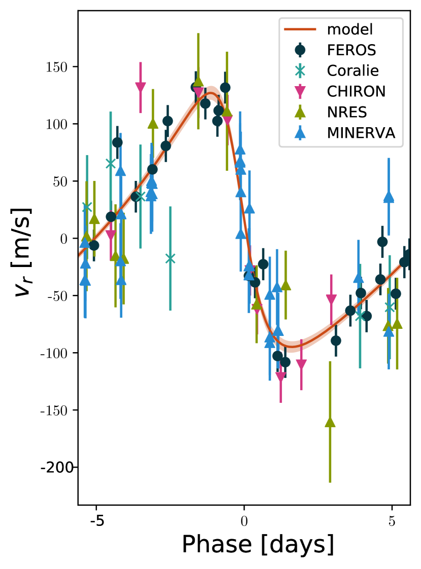
Figure 6: Radial velocities as a function of orbital phase for the five spectroscopic instruments used in this work (FEROS, Coralie, CHIRON, NRES, Minerva). Note that we use a single symbol for Minerva but the observations were made with three different telescopes in the array. The error bars include the posterior values for the jitter terms.

4 Discussion

We put TOI-677 b in the context of the population of known, well characterized transiting exoplanets in Figure 7, where we show a scatter plot of planetary mass versus planetary radius, coding with color the equilibrium temperature. The incident flux for TOI-677 b is $\approx 3\times 10^{8}$ erg s^-1 cm^-2, very close to the value of $\approx 2\times 10^{8}$ erg s^-1 cm^-2 below which it has been shown that the effects of irradiation on the planetary radius are negligible (e.g. Demory & Seager, 2011). The radius of TOI-677 b is in line with what is expected for a gas giant with a core of $M_{C}=10{\rm M}_{\oplus}$ according to the standard models of Fortney et al. (2007). This underscores the value of warm giants, whose structure can be modeled without the complications of an incident flux resulting in radius inflation (Kovács et al., 2010; Demory & Seager, 2011). Figure 7 also shows that TOI-677 b, having a transmission spectroscopy metric (TSM, Kempton et al., 2018) of $\approx$100, is not a particularly well suited target of transmission spectroscopy studies, if compared with the rest of the population of close-in giant planets.

In Figure 8 we plot the same population of well-characterized planets in the period–eccentricity plane, coding the planetary mass with the symbol size. It is apparent that TOI-677 b lies in a part of this plane that is still sparsely populated. The eccentricity of exoplanets is very low for close-in systems, and starts to grow for periods $P\gtrsim 4$ d. With an eccentricity of $e=0.435\pm 0.024$, TOI-677 b lies in the upper range of eccentricity values for planets with similar periods in the currently known sample. Besides the significant eccentricity of the orbit of TOI-677 b  the presence of a long term trend in the radial velocities is interesting in the context of migration mechanisms of giant planets. Warm jupiters can be formed via secular gravitational interactions with an outer planet followed by tidal interactions with the star in the high eccentricity stage of the secular cycle (e.g. Kozai, 1962). In this context, Dong et al. (2014) predicts that in order to overcome the precession caused by general relativity, the warm jupiters produced via this mechanism should have outer planets at relatively short orbital distances that can be detected with a radial velocity monitoring. At the moment we cannot provide meaningful constraints on a potential outer companion. We will continue to monitor the system with radial velocities to determine the exact nature of the long term radial velocity we uncovered.

Figure 7: Mass – Radius diagram for the population of well characterized transiting planets (Southworth, 2011). The point corresponding to TOI-677 b is indicated with a dashed line. The color represents the equilibrium temperature of the planet, while the size scales down with the transmission spectroscopy metric as defined by Kempton et al. (2018). The dashed gray lines correspond to isodensity curves for 0.3, 3 and 30 g cm^-3, respectively. The solid line corresponds to the predicted radius using the models of Fortney et al. (2007) for a planet with a 10 ${\rm M}_{\oplus}$ central core.

The determination of the orbital obliquity of transiting planets through the Rossiter-McLaughlin (R-M) effect, particularly for planets with orbital periods longer than $\approx$10 days, provides a powerful tool to constrain migration theories (Petrovich & Tremaine, 2016). With a sizable $v\sin{i}$ of $7.80\pm 0.19$ ${\rm km\,s^{-1}}$ and a bright magnitude of $V=9.8$ mag, TOI-677 b is a prime target to perform a measurement of the projected angle between the stellar and orbital angular momenta. Specifically, the expected semi-amplitude of the R-M signal for TOI-677 b in the case of an aligned orbit is of K${}_{R-M}=70\pm 10$ ms^-1. While still based on a very limited population, the current obliquity distribution of transiting planets with similar periods as TOI-677 b seems to follow a similar behaviour to that of the eccentricity distribution, with a large spread in their values. Current discoveries include aligned systems like WASP-84b (Anderson et al., 2015) and HAT-P-17b (Fulton et al., 2013), mildly misaligned systems (WASP-117b, Lendl et al., 2014), and also others that are even retrograde (WASP-8b, Queloz et al., 2010). The measurement of the obliquity of TOI-677 b will increment this small sample and help in further understanding how close-in giant planets form.

Figure 8: Period – Eccentricity diagram for the population of well characterized transiting planets. The point corresponding to TOI-677 b is indicated with a dashed line. The size scales with the mass of the planet. The black points with error bars are the average eccentricities of the sample in bins that are equally spaced in $\log(P)$ for $P<100$ d.

Table 3: Relative photometry for TOI-677.

BJD	f	$\sigma_{\rm f}$	Instrument
(2,400,000$+$)	ppt	ppt
58547.001330	-0.199	0.789	TESS
58547.002719	1.058	0.790	TESS
58547.004108	0.339	0.789	TESS
58547.005496	-1.082	0.790	TESS
58547.006885	0.377	0.790	TESS
58547.008274	1.051	0.790	TESS
58547.009663	0.314	0.789	TESS
58547.011052	1.058	0.790	TESS
58547.012441	-0.483	0.790	TESS
58547.013830	0.617	0.789	TESS
58547.015219	-0.675	0.790	TESS
58547.016608	-0.039	0.789	TESS
58547.017997	0.166	0.790	TESS
58547.019386	0.393	0.788	TESS
58547.020774	-0.916	0.790	TESS
58547.022163	-1.167	0.789	TESS
58547.023552	2.311	0.790	TESS
58547.024941	1.251	0.790	TESS
58547.026330	0.043	0.789	TESS
58547.027719	-0.603	0.790	TESS

Table 4: Radial velocities and bisector spans for TOI-677.

BJD	RV	$\sigma_{\rm RV}$	BIS	$\sigma_{\rm BIS}$	Instrument
(2,400,000$+$)	(m s-1)	(m s-1)	(m s-1)	(m s-1)
58615.051551	-26.62	5.4	…	…	Minerva_T3
58615.051551	-70.76	5.3	…	…	Minerva_T4
58615.072962	-26.25	5.4	…	…	Minerva_T3
58615.072962	-12.28	5.3	…	…	Minerva_T4
58616.005135	-43.36	5.4	…	…	Minerva_T3
58616.026546	-81.33	5.4	…	…	Minerva_T3
58616.047945	-81.42	5.4	…	…	Minerva_T3
58618.484021	-107.13	12.0	34	9	FEROS
58619.499881	-78.23	9.6	47	8	FEROS
58620.482581	-54.73	11.3	14	9	FEROS
58621.616231	42.13	23.5	-51	20	Coralie
58621.623201	-14.62	13.3	…	…	CHIRON
58621.628071	-20.13	13.3	23	10	FEROS
58621.948677	-47.48	5.2	…	…	Minerva_T4
58621.948677	67.59	5.4	…	…	Minerva_T3
58621.970088	-6.47	5.4	…	…	Minerva_T4
58621.970088	-27.69	5.4	…	…	Minerva_T3
58622.467171	-1.33	9.8	35	8	FEROS
58622.623371	14.93	23.1	86	20	Coralie
58622.626601	116.18	24.5	…	…	CHIRON

References

- Addison et al. (2019) Addison, B., Wright, D. J., Wittenmyer, R. A., et al. 2019, arXiv e-prints, arXiv:1901.11231
- Albrecht et al. (2012) Albrecht, S., Winn, J. N., Johnson, J. A., et al. 2012, ApJ, 757, 18
- Anderson et al. (2015) Anderson, D. R., Triaud, A. H. M. J., Turner, O. D., et al. 2015, ApJ, 800, L9
- Anglada-Escudé & Butler (2012) Anglada-Escudé, G., & Butler, R. P. 2012, ApJS, 200, 15
- Astropy Collaboration et al. (2013) Astropy Collaboration, Robitaille, T. P., Tollerud, E. J., et al. 2013, A&A, 558, A33
- Astropy Collaboration et al. (2018) Astropy Collaboration, Price-Whelan, A. M., Sipőcz, B. M., et al. 2018, AJ, 156, 123
- Bakos et al. (2004) Bakos, G., Noyes, R. W., Kovács, G., et al. 2004, PASP, 116, 266
- Bakos et al. (2013) Bakos, G. Á., Csubry, Z., Penev, K., et al. 2013, PASP, 125, 154
- Barclay et al. (2018) Barclay, T., Pepper, J., & Quintana, E. V. 2018, ArXiv e-prints, arXiv:1804.05050
- Borucki et al. (2010) Borucki, W. J., Koch, D., Basri, G., et al. 2010, Science, 327, 977
- Brahm et al. (2017a) Brahm, R., Jordán, A., & Espinoza, N. 2017a, PASP, 129, 034002
- Brahm et al. (2017b) Brahm, R., Jordán, A., Hartman, J., & Bakos, G. 2017b, MNRAS, 467, 971
- Brahm et al. (2015) Brahm, R., Jordán, A., Hartman, J. D., et al. 2015, AJ, 150, 33
- Brahm et al. (2016) Brahm, R., Jordán, A., Bakos, G. Á., et al. 2016, AJ, 151, 89
- Brahm et al. (2019) Brahm, R., Espinoza, N., Jordán, A., et al. 2019, AJ, 158, 45
- Cardelli et al. (1989) Cardelli, J. A., Clayton, G. C., & Mathis, J. S. 1989, ApJ, 345, 245
- Castelli & Kurucz (2004) Castelli, F., & Kurucz, R. L. 2004, ArXiv e-prints, astro
- Dawson (2014) Dawson, R. I. 2014, ApJ, 790, L31
- Dawson & Johnson (2018) Dawson, R. I., & Johnson, J. A. 2018, ArXiv e-prints, arXiv:1801.06117
- Demory & Seager (2011) Demory, B.-O., & Seager, S. 2011, ApJS, 197, 12
- Dong et al. (2014) Dong, S., Katz, B., & Socrates, A. 2014, ApJ, 781, L5
- Engel et al. (2017) Engel, M., Shahaf, S., & Mazeh, T. 2017, Publications of the Astronomical Society of the Pacific, 129, 065002
- Espinoza (2018) Espinoza, N. 2018, Research Notes of the American Astronomical Society, 2, 209
- Espinoza & Jordán (2015) Espinoza, N., & Jordán, A. 2015, MNRAS, 450, 1879
- Espinoza et al. (2018) Espinoza, N., Kossakowski, D., & Brahm, R. 2018, arXiv e-prints, arXiv:1812.08549
- Foreman-Mackey et al. (2019) Foreman-Mackey, D., Czekala, I., Agol, E., et al. 2019, dfm/exoplanet: exoplanet v0.2.0, , , doi:10.5281/zenodo.3359880. https://doi.org/10.5281/zenodo.3359880
- Foreman-Mackey et al. (2013) Foreman-Mackey, D., Hogg, D. W., Lang, D., & Goodman, J. 2013, PASP, 125, 306
- Fortney et al. (2007) Fortney, J. J., Marley, M. S., & Barnes, J. W. 2007, ApJ, 659, 1661
- Fulton et al. (2018) Fulton, B. J., Petigura, E. A., Blunt, S., & Sinukoff, E. 2018, ArXiv e-prints, arXiv:1801.01947
- Fulton et al. (2013) Fulton, B. J., Howard, A. W., Winn, J. N., et al. 2013, ApJ, 772, 80
- Gaia Collaboration et al. (2018) Gaia Collaboration, Brown, A. G. A., Vallenari, A., et al. 2018, ArXiv e-prints, arXiv:1804.09365
- Gaia Collaboration et al. (2016) Gaia Collaboration, Prusti, T., de Bruijne, J. H. J., et al. 2016, A&A, 595, A1
- Gelman et al. (2013) Gelman, A., Carlin, J., Stern, H., et al. 2013, Bayesian Data Analysis, Third Edition, Chapman & Hall/CRC Texts in Statistical Science (Taylor & Francis). https://books.google.cl/books?id=ZXL6AQAAQBAJ
- Hoffman & Gelman (2011) Hoffman, M., & Gelman, A. 2011, Journal of Machine Learning Research, 15
- Huber et al. (2019) Huber, D., Chaplin, W. J., Chontos, A., et al. 2019, AJ, 157, 245
- Husser et al. (2013) Husser, T. O., Wende-von Berg, S., Dreizler, S., et al. 2013, Astronomy and Astrophysics, 553, A6
- Jenkins et al. (2016) Jenkins, J. M., Twicken, J. D., McCauliff, S., et al. 2016, in Proc. SPIE, Vol. 9913, Software and Cyberinfrastructure for Astronomy IV, 99133E
- Jones et al. (2019) Jones, M. I., Brahm, R., Espinoza, N., et al. 2019, A&A, 625, A16
- Jordán et al. (2014) Jordán, A., Brahm, R., Bakos, G. Á., et al. 2014, AJ, 148, 29
- Kaufer et al. (1999) Kaufer, A., Stahl, O., Tubbesing, S., et al. 1999, The Messenger, 95, 8
- Kempton et al. (2018) Kempton, E. M.-R., Bean, J. L., Louie, D. R., et al. 2018, ArXiv e-prints, arXiv:1805.03671
- Kipping (2013) Kipping, D. M. 2013, MNRAS, 435, 2152
- Kovács et al. (2010) Kovács, G., Bakos, G. Á., Hartman, J. D., et al. 2010, ApJ, 724, 866
- Kozai (1962) Kozai, Y. 1962, AJ, 67, 591
- Lendl et al. (2014) Lendl, M., Triaud, A. H. M. J., Anderson, D. R., et al. 2014, A&A, 568, A81
- Li & Winn (2016) Li, G., & Winn, J. N. 2016, ApJ, 818, 5
- Li et al. (2019) Li, J., Tenenbaum, P., Twicken, J. D., et al. 2019, PASP, 131, 024506
- Luger et al. (2019) Luger, R., Agol, E., Foreman-Mackey, D., et al. 2019, AJ, 157, 64
- Mayor et al. (2003) Mayor, M., Pepe, F., Queloz, D., et al. 2003, The Messenger, 114, 20
- Méndez & Rivera-Valentín (2017) Méndez, A., & Rivera-Valentín, E. G. 2017, ApJ, 837, L1
- Miller & Fortney (2011) Miller, N., & Fortney, J. J. 2011, ApJ, 736, L29
- Pepper et al. (2007) Pepper, J., Pogge, R. W., DePoy, D. L., et al. 2007, PASP, 119, 923
- Petrovich & Tremaine (2016) Petrovich, C., & Tremaine, S. 2016, ApJ, 829, 132
- Pollacco et al. (2006) Pollacco, D. L., Skillen, I., Collier Cameron, A., et al. 2006, PASP, 118, 1407
- Queloz et al. (2010) Queloz, D., Anderson, D. R., Collier Cameron, A., et al. 2010, A&A, 517, L1
- Ricker et al. (2015) Ricker, G. R., Winn, J. N., Vanderspek, R., et al. 2015, Journal of Astronomical Telescopes, Instruments, and Systems, 1, 014003
- Rodriguez et al. (2019) Rodriguez, J. E., Quinn, S. N., Huang, C. X., et al. 2019, AJ, 157, 191
- Salvatier et al. (2016) Salvatier, J., Wiecki, T. V., & Fonnesbeck, C. 2016, PeerJ Computer Science, 2, e55
- Siverd et al. (2018) Siverd, R. J., Brown, T. M., Barnes, S., et al. 2018, in Society of Photo-Optical Instrumentation Engineers (SPIE) Conference Series, Vol. 10702, Ground-based and Airborne Instrumentation for Astronomy VII, 107026C
- Smith et al. (2012) Smith, J. C., Stumpe, M. C., Van Cleve, J. E., et al. 2012, PASP, 124, 1000
- Southworth (2011) Southworth, J. 2011, MNRAS, 417, 2166
- Stassun & Torres (2018) Stassun, K. G., & Torres, G. 2018, ApJ, 862, 61
- Stumpe et al. (2014) Stumpe, M. C., Smith, J. C., Catanzarite, J. H., et al. 2014, PASP, 126, 100
- Sullivan et al. (2015) Sullivan, P. W., Winn, J. N., Berta-Thompson, Z. K., et al. 2015, ApJ, 809, 77
- Talens et al. (2017) Talens, G. J. J., Albrecht, S., Spronck, J. F. P., et al. 2017, A&A, 606, A73
- Theano Development Team (2016) Theano Development Team. 2016, arXiv e-prints, abs/1605.02688. http://arxiv.org/abs/1605.02688
- Tokovinin (2018) Tokovinin, A. 2018, PASP, 130, 035002
- Tokovinin et al. (2013) Tokovinin, A., Fischer, D. A., Bonati, M., et al. 2013, PASP, 125, 1336
- Twicken et al. (2018) Twicken, J. D., Catanzarite, J. H., Clarke, B. D., et al. 2018, PASP, 130, 064502
- Wang et al. (2019) Wang, S., Jones, M., Shporer, A., et al. 2019, AJ, 157, 51
- Welch (1967) Welch, P. D. 1967, IEEE Trans. Audio & Electroacoust, 15, 70
- Ziegler et al. (2019) Ziegler, C., Tokovinin, A., Briceno, C., et al. 2019, arXiv e-prints, arXiv:1908.10871