Developments in the position-space approach to the HLbL contribution to the muon $\bm{g-2}$ on the lattice

Abstract:

The measurement of the anomalous magnetic moment of the muon and its prediction allow for a high-precision test of the Standard Model (SM). In this proceedings article we present ongoing work combining lattice QCD and continuum QED in order to determine an important SM contribution to the magnetic moment, the hadronic light-by-light contribution. We compute the quark-connected contribution in the Mainz position-space approach and investigate the long-distance part of our data using calculations of the $\pi^{0}$-pole and charged pion loop contributions.

1 Introduction

One of the most stringent tests of the Standard Model (SM) arises from the measurement of the anomalous magnetic moment of the muon $a_{\mu}$. A tension of about three standard deviations persists between the SM prediction for this quantity and its experimentally measured value. The theory and experimental uncertainties are comparable and at the sub-ppm level, but new experiments such as the “E989 Muon g-2” at Fermilab and the “Muon g-2/EDM” at JPARC expect an improvement in precision by about a factor four in the next few years; see [1] and references therein. It is necessary to reduce the theoretical uncertainty by a comparable amount in order to discern whether the current discrepancy between theory and experiment is a sign of Beyond the Standard Model physics.

The theoretical uncertainty for $a_{\mu}$ is currently dominated by hadronic contributions, namely the hadronic vacuum polarization (HVP) as well as the hadronic light-by-light (HLbL) scattering. It is the latter of these contributions that we will focus on in this proceedings article. We will summarize the methodology and present some preliminary results for the contribution of the quark-connected diagrams to $a_{\mu}^{\text{HLBL}}$ as well as a discussion of finite-volume effects and our use of continuum models to describe the long-distance part of our data. To this end, continuum computations of the $\pi^{0}$-pole and charged pion loop contributions are presented.

2 Position-space method

To compute the HLbL contribution, we make use of the Mainz position-space method, see also references [2, 3, 4, 5, 6]. It divides the problem into a QED part and a QCD part. The QED part is described by a kernel function $\bar{\mathcal{L}}$, that is computed in the continuum and infinite volume, and the QCD part is given by a four-point function $i\widehat{\Pi}$, that is to be obtained with the help of Lattice QCD. The master formula that allows one to compute the HLbL contribution to $a_{\mu}$ reads

$$a_{\mu}^{\rm HLbL} =\frac{me^{6}}{3}\int d^{4}y\Big{[}\int d^{4}x\underbrace{\bar{\cal L}_{[\rho,\sigma];\mu\nu\lambda}(x,y)}_{\rm QED}\;\underbrace{i\widehat{\Pi}_{\rho;\mu\nu\lambda\sigma}(x,y)}_{\rm QCD}\Big{]}.$$ (1)

$$i\widehat{\Pi}_{\rho;\mu\nu\lambda\sigma}(x,y) =\int d^{4}z\;(-z_{\rho})\widetilde{\Pi}_{\mu\nu\sigma\lambda}(x,y,z),\quad\widetilde{\Pi}_{\mu\nu\sigma\lambda}(x,y,z)=\big{\langle}\,j_{\mu}(x)\,j_{\nu}(y)\,j_{\sigma}(z)\,j_{\lambda}(0)\big{\rangle}\,,$$ (2)

where $m$ is the mass of the muon and the $j_{\mu}(x)$ are the quark electromagnetic currents.

The kernel $\bar{\mathcal{L}}$ is not unique. Other valid kernels can be obtained by adding or subtracting terms that vanish after the $x$ and $y$ integrations in the master formula (1). Such subtractions were first introduced in [7], where it was shown that discretization effects can be drastically reduced by choosing kernels that vanish when some of the vertices coincide. Exploiting $\int_{x}i\widehat{\Pi}(x,y)=\int_{y}i\widehat{\Pi}(x,y)=0\,,$ we have tested the usefulness of the subtracted kernels $\mathcal{L}^{(1-3)}$,

$$\mathcal{L}^{(0)}= \bar{\mathcal{L}}(x,y)\,,\quad\text{(standard kernel)}$$ (3)

$$\mathcal{L}^{(1)}= \bar{\mathcal{L}}(x,y)-\frac{1}{2}\bar{\mathcal{L}}(x,x)-\frac{1}{2}\bar{\mathcal{L}}(y,y)\,,$$ (4)

$$\mathcal{L}^{(2)}= \bar{\mathcal{L}}(x,y)-\bar{\mathcal{L}}(0,y)-\bar{\mathcal{L}}(x,0)\,,$$ (5)

$$\mathcal{L}^{(3)}= \bar{\mathcal{L}}(x,y)-\bar{\mathcal{L}}(0,y)-\bar{\mathcal{L}}(x,x)+\bar{\mathcal{L}}(0,x)\,,$$ (6)

that obey the following properties:

$$\mathcal{L}^{(0)}(0,0)=0\,,\quad\mathcal{L}^{(1)}(x,x)=0\,,\quad\mathcal{L}^{(2)}(0,y)=\mathcal{L}^{(2)}(x,0)=0\,,\quad\mathcal{L}^{(3)}(x,x)=\mathcal{L}^{(3)}(0,y)=0\,.$$ (7)

The left panel of Fig. 1 displays the integrands $f(|y|)$ of the final integration over $|y|$ corresponding to the different kernels, for the neutral pion pole contribution with a vector-meson-dominance (VMD) model of the pion transition form factor. Compared to the standard kernel, $\mathcal{L}^{(2)}$ and $\mathcal{L}^{(3)}$ have less pronounced peaks at short distances and approach zero faster at long distances. We expect these subtracted kernels to have smaller lattice artifacts and therefore to be favorable in lattice computations.

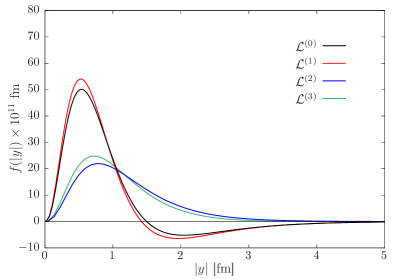
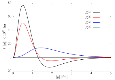
Figure 1: The integrand for the $\pi^{0}$-pole contribution based on the standard kernel $\mathcal{L}^{(0)}$ and the subtracted kernels $\mathcal{L}^{(1,2,3)}$ at $m_{\pi}=$300\text{\,}\mathrm{M}\mathrm{e}\mathrm{V}$$, using method 1 (left panel) and method 2 (right panel). In the right-hand plot, the $\mathcal{L}^{(3)}$ curve is hidden behind the $\mathcal{L}^{(2)}$ curve. The continuum calculation is performed using the VMD model for the pion transition form factor.

The quark-connected part of the four-point function $i\widehat{\Pi}$, involves three different contractions. Computing all three of them and applying Eq. (1) amounts to what we call ‘method 1’. In a lattice implementation of this method, for $N$ evaluations of the $y$ integrand, $1+N$ propagators and $6(1+N)$ sequential propagators are needed. If $\Pi^{(1)}_{\mu\nu\sigma\lambda}(x,y,z)\equiv-2{\rm ReTr}\{S(0,x)\gamma_{\mu}S(x,y)\gamma_{\nu}S(y,z)\gamma_{\sigma}S(z,0)\gamma_{\lambda}\}$, where the $S(x,y)$ are propagators, represents one of the Wick contractions of the quark-connected part $\widetilde{\Pi}^{c}_{\mu\nu\sigma\lambda}(x,y,z)$, we can write (for any given background gauge field)

$$\widetilde{\Pi}^{c}_{\mu\nu\sigma\lambda}(x,y,z)=\Pi^{(1)}_{\mu\nu\sigma\lambda}(x,y,z)+\Pi^{(1)}_{\nu\mu\sigma\lambda}(y,x,z)+\Pi^{(1)}_{\nu\sigma\mu\lambda}(y,z,x).$$ (8)

Note that $\partial_{\mu}(x)\widetilde{\Pi}^{c}_{\mu\nu\sigma\lambda}(x,y,z)=0$ for all $x$. The computation can be arranged in a different way, such that only the contraction $\Pi^{(1)}$ is computed and the others are implemented by permuting the way that the photons are attached to the vertices of the four-point function. We call this method 2, which reads

$$a_{\mu}^{\text{HLbL,c}}=\frac{me^{6}}{3}\int_{y,x,z}\Big{(} [\bar{\mathcal{L}}_{[\rho,\sigma];\mu\nu\lambda}(x,y)+\bar{\mathcal{L}}_{[\rho,\sigma];\nu\mu\lambda}(y,x)-\bar{\mathcal{L}}_{[\rho,\sigma];\lambda\nu\mu}(x,x-y)](-z_{\rho})\,\Pi^{(1)}_{\mu\nu\sigma\lambda}(x,y,z)$$

$$+\bar{\mathcal{L}}_{[\rho,\sigma];\lambda\nu\mu}(x,x-y)\,(-x_{\rho})\Pi^{(1)}_{\mu\nu\sigma\lambda}(x,y,z)\Big{)}.$$ (9)

A diagrammatic representation and the integrands for both methods are shown in Figs. 2 and 1. While method 2 requires the calculation of far fewer propagators, its integrand receives contributions from the exchange of resonances odd under charge conjugation, which cancel out upon fully integrating over $x,y,z$.

(a)

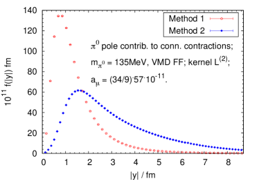
(b)

Figure 2: (a) Contractions needed to compute $g-2$. Upper row: The three connected Wick contractions needed in method 1. Bottom row: In method 2 the different contraction types are implemented in the QED part of the diagram. (b) Comparison of the integrands for method 1 and method 2 for the neutral pion pole contribution with a transition form factor given by the VMD model.

3 Lattice results

The results described in this section are obtained with kernel $\mathcal{L}^{(2)}$, which we expect to reduce lattice artifacts. For our lattice calculations, which are based on the ensembles listed in Table 1, we use method 2 to reduce the number of required inversions of the Dirac operator. From Fig. 3, we observe that we achieve good statistical precision for small $|y|$, but at larger distances the signal degrades rapidly.

The ensembles N203 and H102 have a similar pion mass of about $350\text{\,}\mathrm{M}\mathrm{e}\mathrm{V}$ but differ by their lattice spacing and the physical volume of the boxes. At this pion mass, the discretization effects can be resolved, cf. Fig. 3a. As the ensembles N203, N200, and D200 all have the same lattice spacing, comparing them allows us to explore the pion-mass dependence of $a_{\mu}$, which exhibits a mild increase with decreasing pion mass, see Fig. 3c. Finite-volume effects become more relevant at long distances and precise knowledge of the long-distance tail is very important. As H105 and N101 differ only in their physical volume, a comparison of their long-distance behavior allows us to understand the magnitude of our finite-volume effects. These two ensembles seem roughly consistent at large distances in Fig. 3b, although their error bars indicate that more statistics are needed.

Label $L^{3}\times T$ $a~{}$[fm] $m_{\pi}~{}$[MeV] $m_{\pi}L$ $L$ [fm] $\#$confs H102 $32^{3}\times 96$ 0.08636 $354(5)$ 5.0 2.8 900 H105 $32^{3}\times 96$ $284(4)$ 3.9 2.8 1000 N101 $48^{3}\times 128$ $282(4)$ 5.9 4.1 400 N203 $48^{3}\times 128$ 0.06426 $345(4)$ 5.4 3.1 750 N200 $48^{3}\times 128$ $282(3)$ 4.4 3.1 800 D200 $64^{3}\times 128$ $200(2)$ 4.2 4.1 1100

Table 1: CLS $N_{f}=2+1$ ensembles used in this work.

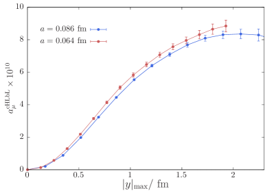
(a)

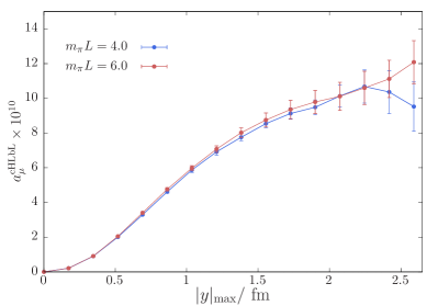
(b)

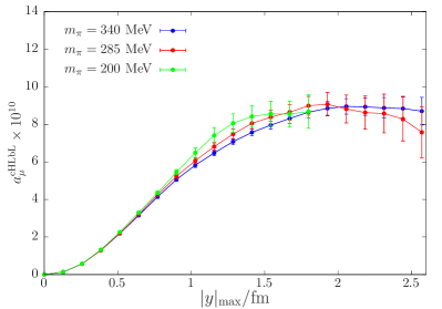
(c)

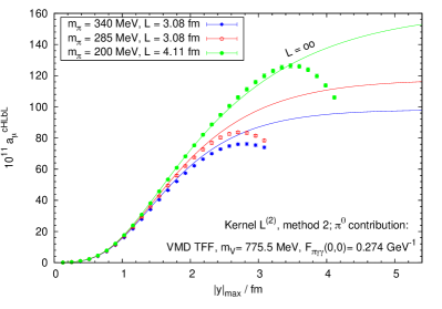
(d)

Figure 3: (a) Discretization effects on the lattices H102 and N203. (b) Finite-size effects on the H105 and N101 lattices. (c) Pion-mass dependence on the N203, N200 and D200 lattices. (d) Pion-mass dependence and finite-size effects for the $\pi^{0}$-pole contribution. The curves represent infinite-volume and the points finite-volume results.

4 Pion mass dependence and finite-size effects

The lattice results presented in the previous section exhibit a mild upward trend for decreasing pion mass. For the neutral pion pole prediction calculated in finite volume we obtain a similar behavior. However in infinite volume the integral extends to longer distances and correspondingly shows a stronger increase as $m_{\pi}$ is reduced; see Fig. 3d. This illustrates the importance of understanding the tail of the integrand semi-analytically.

We have thus identified two sources of finite volume effects: one is the truncation of the $y$-integral, and the other comes from the finite-size effect on the lattice integrand itself. Both artifacts can be corrected for by semi-analytic continuum computations (Fig. 3d). In the small-distance regime the corrections are small and the lattice data can be used directly. For longer distances, where the finite-size effect becomes larger, the $\pi^{0}$-pole contribution becomes increasingly dominant and we can use the continuum computation to model the long-distance tail of the $y$ integrand.

Figure 4 shows the lattice integrand for the N203 lattice and the corresponding integrand for the $\pi^{0}$-pole contribution, also computed with method 2. We note that $\Pi^{(1)}_{\mu\nu\sigma\lambda}(x,y,z)$ does not contain the pion-level diagram in which the $\pi^{0}$ propagates between the pair $(0,y)$ and the pair $(x,z)$ of vertices, and that the normalization of the two other $\pi^{0}$-pole diagrams is such that $\tilde{\Pi}^{c}_{\mu\nu\sigma\lambda}$ contains the same $\pi^{0}$ contribution as $\tilde{\Pi}_{\mu\nu\sigma\lambda}$, enhanced (in the SU(2)_f case) by the charge factor $34/9$. In Fig. 4 we observe effects that are not described by the $\pi^{0}$-pole prediction at short distances. At larger distances, we need to collect more statistics to test against the $\pi^{0}$-pole prediction. The data lie below the prediction, suggesting that there may be a negative contribution to the integrand that is non-negligible at $|y|=1.5{\rm\,fm}$.

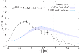
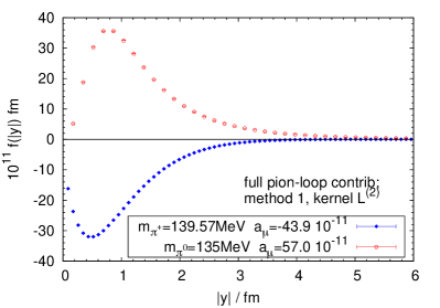
Figure 4: Left: comparison between the integrand from ensemble N203 and the integrand for the $\pi^{0}$-pole contribution, both computed with method 2 and kernel ${\cal L}^{(2)}$. The infinite-volume band covers the normalization factors from $3$ to $34/9$ [8], the $\pi^{0}$ finite-volume points are normalized with the factor $34/9$. Right: pion-pole contribution with a VMD transition form factor (red) and charged pion loop contribution in scalar QED (blue) to $a_{\mu}^{\rm HLbL}$, using method 1.

One contribution to $a_{\mu}^{\rm HLbL}$ that is known to be negative is the charged pion loop. It is also parametrically leading in the chiral limit. Starting from scalar QED in Euclidean space,

$$\mathcal{L}_{\rm E}=(\partial_{\mu}+ieA_{\mu})\phi^{*}(\partial_{\mu}-ieA_{\mu})\phi+m^{2}\phi^{*}\phi+\frac{1}{4}F_{\mu\nu}F_{\mu\nu},$$ (10)

we have performed such a computation in our position-space formulation and successfully reproduced the known charged pion loop contribution [9]. The integrand corresponding to method 1 is shown in the right panel of  Fig. 4 for physical pion masses. Indeed the pion loop contribution is of comparable size and opposite in sign to the neutral pion pole contribution. It is also of shorter range, and if it were further suppressed by realistic form factors, it would be unlikely to produce the negative contribution suggested by the left panel of Fig. 4.

5 Conclusions

The Mainz position-space approach is a method for computing $a_{\mu}^{\text{HLbL}}$ using continuum, infinite-volume QED combined with lattice QCD. The correctness of the kernel has by now successfully been tested on the fermion loop, the pion loop as well as on the neutral pion pole contribution. Semi-analytic computations based on the $\pi^{0}$-pole contribution in finite volume are important to control the artifacts that stem from the finite size of the box.

The freedom one has in choosing the QED kernel without affecting $a_{\mu}^{\text{HLbL}}$ allows for a suppression of certain discretization effects via subtractions; see Eqs. (5–6). However, the finite-size effects then turn out to be challenging. Therefore we are investigating the benefit of a new class of kernels

$${\cal L}^{(2,\bar{\lambda})}_{\rho\sigma;\mu\nu\lambda}={\cal L}^{(0)}_{\rho\sigma;\mu\nu\lambda}(x,y)-\partial_{\mu}^{(x)}\Big{(}x_{\alpha}\,e^{-\bar{\lambda}m_{\mu}^{2}x^{2}/2}\Big{)}\;{\cal L}^{(0)}_{\rho\sigma;\alpha\nu\lambda}(0,y)-\partial_{\nu}^{(y)}\Big{(}y_{\alpha}\,e^{-\bar{\lambda}m_{\mu}^{2}y^{2}/2}\Big{)}\;{\cal L}^{(0)}_{\rho\sigma;\mu\alpha\lambda}(x,0),$$ (11)

which reduces to ${\cal L}^{(2)}$ for $\bar{\lambda}=0$, shares its property of vanishing whenever $x$ or $y$ does, but does not qualitatively alter the long-distance behavior of the original kernel ${\cal L}^{(0)}$.

Acknowledgments   This work is supported by the Deutsche Forschungsgemeinschaft (DFG) through the Collaborative Research Centre 1044 and the European Research Council (ERC) under the European Union’s Horizon 2020 research and innovation programme through grant agreement 771971-SIMDAMA.

References

- [1] Fred Jegerlehner. Muon theory: The hadronic part. EPJ Web Conf., 166 (2018) 00022.
- [2] Jeremy Green, Nils Asmussen, Oleksii Gryniuk, Georg von Hippel, Harvey B. Meyer, Andreas Nyffeler, and Vladimir Pascalutsa. Direct calculation of hadronic light-by-light scattering. PoS, LATTICE2015 (2016) 109.
- [3] Nils Asmussen, Jeremy Green, Harvey B. Meyer, and Andreas Nyffeler. Position-space approach to hadronic light-by-light scattering in the muon on the lattice. PoS, LATTICE2016 (2016) 164.
- [4] Nils Asmussen, Antoine Gerardin, Jeremy Green, Oleksii Gryniuk, Georg von Hippel, Harvey B. Meyer, Andreas Nyffeler, Vladimir Pascalutsa, and Hartmut Wittig. Hadronic light-by-light scattering contribution to the muon on the lattice. EPJ Web Conf. 179 (2018) 01017.
- [5] Nils Asmussen, Antoine Gérardin, Harvey B. Meyer, and Andreas Nyffeler. Exploratory studies for the position-space approach to hadronic light-by-light scattering in the muon –2. EPJ Web Conf. 175 (2018) 06023.
- [6] Nils Asmussen, Antoine Gérardin, Andreas Nyffeler, and Harvey B. Meyer. Hadronic light-by-light scattering in the anomalous magnetic moment of the muon. SciPost Phys. Proc. 1 (2019) 031.
- [7] Thomas Blum, Norman Christ, Masashi Hayakawa, Taku Izubuchi, Luchang Jin, Chulwoo Jung, and Christoph Lehner. Using infinite volume, continuum QED and lattice QCD for the hadronic light-by-light contribution to the muon anomalous magnetic moment. Phys. Rev., D 96 (2017) no. 3, 034515.
- [8] J. Bijnens and J. Relefors. Pion light-by-light contributions to the muon –2. JHEP 1609 (2016) 113.
- [9] J. H. Kühn, A. I. Onishchenko, A. A. Pivovarov and O. L. Veretin. Heavy mass expansion, light by light scattering and the anomalous magnetic moment of the muon. Phys. Rev. D 68 (2003) 033018