A Capsule Network-based Model for Learning Node Embeddings

Abstract.

In this paper, we focus on learning low-dimensional embeddings for nodes in graph-structured data. To achieve this, we propose Caps2NE – a new unsupervised embedding model leveraging a network of two capsule layers. Caps2NE induces a routing process to aggregate feature vectors of context neighbors of a given target node at the first capsule layer, then feed these features into the second capsule layer to infer a plausible embedding for the target node. Experimental results show that our proposed Caps2NE obtains state-of-the-art performances on benchmark datasets for the node classification task. Our code is available at: https://github.com/daiquocnguyen/Caps2NE.

1. Introduction

Numerous real-world and scientific data are represented in forms of graphs, e.g. data from knowledge graphs, recommender systems, social and citation networks as well as telecommunication and biological networks (Battaglia et al., 2018; Chen et al., 2018). Recent years have witnessed many successful downstream applications of utilizing the graph-structured data such as for improving information extraction and text classification systems (Kipf and Welling, 2017), traffic learning and forecasting (Cui et al., 2018) and for advertising and recommending relevant items to users (Ying et al., 2018; Wang et al., 2018). This is largely boosted by a surge of methodologies that learn embedding representations to encode graph structures (Cai et al., 2018).

One of the most important tasks in learning graph representations is to learn low-dimensional embeddings for nodes in the graph-structured data (Zhang et al., 2020). These embedding vectors can then be used in a downstream task such as node classification, i.e., using the learned node embeddings as feature inputs to train a classifier to predict node labels (Hamilton et al., 2017).

A simple and effective approach is to treat each node as a word token and each graph as a text collection; hence we can apply a word embedding model such as Word2Vec (Mikolov et al., 2013) to learn node embeddings such as DeepWalk (Perozzi et al., 2014) and Node2Vec (Grover and Leskovec, 2016). Recent work has developed deep neural networks (DNN) for the node classification task, e.g., GCN (Kipf and Welling, 2017), GraphSAGE (Hamilton et al., 2017) and GAT (Veličković et al., 2018). We see that the DNN-based approaches are showing state-of-the-art performances, but not well-efficient to exploit the structural dependencies among nodes.

In this paper, inspired by the advanced capsule networks (Sabour et al., 2017), we present Caps2NE – a new unsupervised embedding model that adapts capsule network to learn node embeddings. Caps2NE aims to capture $h$-hops context neighbors to predict a target node. In particular, Caps2NE consists of two capsule layers with connections from the first to the second layer, but no connections within layers. The first layer constructs capsules to encapsulate context neighbors. Then a routing process is used to aggregate the feature information from capsules in the first layer to only one capsule in the second layer. After that, the second layer produces a continuous vector which is used to infer an embedding for the target node. Note that encapsulating the context neighbors into the corresponding capsules aims to preserve node properties more efficiently. And the routing process aims to generate high-level features to infer plausible node embeddings effectively.

Our main contributions are as follows:

• We investigate the advanced use of capsule networks for the graph-structured data and propose a new embedding model Caps2NE to learn node embeddings.

• We evaluate the performance of the proposed Caps2NE on benchmark datasets for the node classification task.

• The experimental results show that that our Caps2NE produces state-of-the-art accuracy results on these datasets.

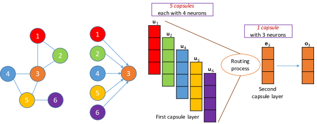
Figure 1. Processes in our Caps2NE with $q=6,d=4,k=3$ for an illustration purpose. Note that in this illustration, we use numbered subscripts to denote nodes themselves, not indexes of nodes or capsules. The indexes of capsules are fixed from 1 to $(q-1)$, not depending on the indexes of the context neighbors. With $\mathsf{v}$ be the target node 3, we have $\mathsf{C}_{\mathsf{v}}=$ $\{\mathsf{v}_{1}=$ 1, $\mathsf{v}_{2}=$ 2, $\mathsf{v}_{3}=$ 4, $\mathsf{v}_{4}=$ 5, $\mathsf{v}_{5}=$ 6$\}$.

2. The proposed Caps2NE

This section presents our Caps2NE model. In particular, we detail how to sample data from an input graph, then how to construct Caps2NE to learn node embeddings.

Definition 1. A network graph $\mathcal{G}$ is defined as $\mathcal{G}=(\mathcal{V},\mathcal{E})$, in which $\mathcal{V}$ is a set of nodes, $\mathcal{E}\subseteq\{(\mathsf{v},\mathsf{v^{\prime}})|\mathsf{v},\mathsf{v^{\prime}}\in\mathcal{V}\}$ is a set of edges, and each node $\mathsf{v}\in\mathcal{V}$ is associated with a feature vector $\boldsymbol{x}_{\mathsf{v}}\in\mathbb{R}^{d}$. We aim to learn a node embedding $\boldsymbol{\mathsf{o}}_{\mathsf{v}}$ for each node $\mathsf{v}$.

Sampling input pairs. We follow Perozzi et al. (2014) to uniformly sample a number $T$ of random walks of length $q$ for every node in $\mathcal{V}$. From each random walk, we randomly sample a target node $\mathsf{v}$, treat $(q-1)$ remaining nodes as the context neighbors of node $\mathsf{v}$, and construct an input pair of ($\mathsf{C}_{\mathsf{v}}$, $\mathsf{v}$), where we denote $\mathsf{C}_{\mathsf{v}}$ be the list of context neighbors $\mathsf{v}_{i}$ of the target node $\mathsf{v}$ (here, $i\in\{1,2,...,q-1\}$ and $|\mathsf{C}_{\mathsf{v}}|=q-1$).

Figure 1 shows an example of a graph consisting of 6 nodes. If we sample a random walk of length $q=6$ for node $1$ such as $\{1,2,3,4,5,6\}$ and select node $3$ as the target node $\mathsf{v}$, then the remaining nodes $\{1,2,4,5,6\}$ are treated as the context neighbors of node $3$, i.e., $\mathsf{C}_{\mathsf{v}}=$ $\{\mathsf{v}_{1}=$ 1, $\mathsf{v}_{2}=$ 2, $\mathsf{v}_{3}=$ 4, $\mathsf{v}_{4}=$ 5, $\mathsf{v}_{5}=$ 6$\}$.

Definition 2. A capsule is a group of neurons. A capsule layer is a group of capsules without connections among capsules in the same layer (Sabour et al., 2017). Two continuous capsule layer is connected using a routing process.

Constructing Caps2NE. We build our Caps2NE with two capsule layers. In the first layer, we construct $(q-1)$ capsules, where the feature vector of each context neighbor $\mathsf{v}_{i}$ is encapsulated by the $i$-th corresponding capsule (with $i\in\{1,2,...,q-1\}$). In the second layer, we construct one capsule to produce a vector representation which is then used to infer an embedding for the target node $\mathsf{v}$.

The first capsule layer consists of $(q-1)$ capsules, in which the $i$-th capsule use a non-linear squashing function to transform the feature vector $\boldsymbol{x}_{\mathsf{v}_{i}}$ of the context neighbor $\mathsf{v}_{i}$ into $\boldsymbol{\mathsf{u}}_{\mathsf{v}_{i}}^{(i)}$ as:

(1) $$\boldsymbol{\mathsf{u}}_{\mathsf{v}_{i}}^{(i)}=\mathsf{squash}\left(\boldsymbol{x}_{\mathsf{v}_{i}}\right)=\frac{\|\boldsymbol{x}_{\mathsf{v}_{i}}\|^{2}}{1+\|\boldsymbol{x}_{\mathsf{v}_{i}}\|^{2}}\frac{\boldsymbol{x}_{\mathsf{v}_{i}}}{\|\boldsymbol{x}_{\mathsf{v}_{i}}\|}$$

The squashing function ensures that the orientation of each feature vector is unchanged while its length is scaled down to below 1.

Vectors $\boldsymbol{\mathsf{u}}_{\mathsf{v}_{i}}^{(i)}$ are then linearly transformed using weight matrices $\textbf{W}_{i}\in\mathbb{R}^{k\times d}$ to produce vectors $\hat{\boldsymbol{\mathsf{u}}}_{\mathsf{v}_{i}}^{(i)}\in\mathbb{R}^{k}$. These vectors $\hat{\boldsymbol{\mathsf{u}}}_{\mathsf{v}_{i}}^{(i)}$ are weighted to sum up to return a vector $\boldsymbol{\mathsf{s}}_{\mathsf{v}}\in\mathbb{R}^{k}$ for the capsule in the second layer (recall that the second layer consists of only one capsule). This capsule then performs the non-linear squashing function to produce a vector $\boldsymbol{\mathsf{e}}_{\mathsf{v}}\in\mathbb{R}^{k}$. Formally, we have:

(2) $$\boldsymbol{\mathsf{e}}_{\mathsf{v}}=\mathsf{squash}\left(\boldsymbol{\mathsf{s}}_{\mathsf{v}}\right)\ \ ;\ \ \boldsymbol{\mathsf{s}}_{\mathsf{v}}=\sum_{i}c_{i}\hat{\boldsymbol{\mathsf{u}}}_{\mathsf{v}_{i}}^{(i)}\ \ ;\ \ \hat{\boldsymbol{\mathsf{u}}}_{\mathsf{v}_{i}}^{(i)}=\textbf{W}_{i}\boldsymbol{\mathsf{u}}_{\mathsf{v}_{i}}^{(i)}$$

where $c_{i}$ are coupling coefficients determined by the routing process as presented in Algorithm 1. Here, $c_{i}$ aims to weight $\boldsymbol{\mathsf{u}}_{\mathsf{v}_{i}}^{(i)}$ of the $i$-th capsule in the first layer.

As we use one capsule in the second layer, we make two differences in our routing process in Algorithm 1: (i) we apply $\mathsf{softmax}$ in a direction from all capsules in the previous layer to each of capsules in the next layer, (ii) thus, we propose a new update rule ($b_{i}\leftarrow\hat{\boldsymbol{\mathsf{u}}}_{\mathsf{v}_{i}}^{(i)}\cdot\boldsymbol{\mathsf{e}}_{\mathsf{v}}$) instead of employing ($b_{i}\leftarrow b_{i}+\hat{\boldsymbol{\mathsf{u}}}_{\mathsf{v}_{i}}^{(i)}\cdot\boldsymbol{\mathsf{e}}_{\mathsf{v}}$) originally used by Sabour et al. (2017).

1 for i = 1, 2, …, q-1 do

2       $b_{i}\leftarrow$ 0

3for $\mathsf{iteration}$ = 1, 2, …, m do

4       $\boldsymbol{\mathsf{c}}\leftarrow\mathsf{softmax}\left(\boldsymbol{\mathsf{b}}\right)$

5      $\boldsymbol{\mathsf{s}}_{\mathsf{v}}\leftarrow\sum_{i}c_{i}\hat{\boldsymbol{\mathsf{u}}}_{\mathsf{v}_{i}}^{(i)}$

6      $\boldsymbol{\mathsf{e}}_{\mathsf{v}}\leftarrow\mathsf{squash}\left(\boldsymbol{\mathsf{s}}_{\mathsf{v}}\right)$

7      for i = 1, 2, …, q-1 do

8             $b_{i}\leftarrow\hat{\boldsymbol{\mathsf{u}}}_{\mathsf{v}_{i}}^{(i)}\cdot\boldsymbol{\mathsf{e}}_{\mathsf{v}}$

9      

Algorithm 1 The Caps2NE routing process.

Learning model parameters. The vector representation $\boldsymbol{\mathsf{e}}_{\mathsf{v}}$ is then used to infer the final embedding $\boldsymbol{\mathsf{o}}_{\mathsf{v}}\in\mathbb{R}^{k}$ of the target node $\mathsf{v}$, as shown in Equation 3. We learn all model parameters (including the node embeddings $\boldsymbol{\mathsf{o}}_{\mathsf{v}}$) by minimizing the sampled softmax loss function (Jean et al., 2015) applied to the target node $\mathsf{v}$ as:

(3) $$\mathcal{L}_{\mathsf{Caps2NE}}\left(\mathsf{v}\right)=-\log\frac{\exp(\boldsymbol{\mathsf{o}}_{\mathsf{v}}^{\mathsf{T}}\boldsymbol{\mathsf{e}}_{\mathsf{v}})}{\sum_{\mathsf{v^{\prime}}\in\mathcal{V^{\prime}}}\exp(\boldsymbol{\mathsf{o}}_{\mathsf{v^{\prime}}}^{\mathsf{T}}\boldsymbol{\mathsf{e}}_{\mathsf{v}})}$$

where $\mathcal{V^{\prime}}$ is a subset sampled from $\mathcal{V}$.

1 Input: A network graph $\mathcal{G}=(\mathcal{V},\mathcal{E})$

2for $\mathsf{v}\in\mathcal{V}$ do

3       Sample $T$ random walks of length $q$ starting at $\mathsf{v}$

4

5for each $\mathsf{random\ walk}$ do

6       Sample a node $\mathsf{v}$ as a target node

7      $\mathsf{C}_{\mathsf{v}}\leftarrow$ Remaining nodes

8      for i = 1, 2, …, q-1 do

9             $\boldsymbol{\mathsf{u}}_{\mathsf{v}_{i}}^{(i)}\leftarrow\mathsf{squash}\left(\boldsymbol{x}_{\mathsf{v}_{i}}\right)\quad\forall\mathsf{v}_{i}\in\mathsf{C}_{\mathsf{v}}$

10      

11      $\boldsymbol{\mathsf{e}}_{\mathsf{v}}\leftarrow\textsc{Routing}\left(\left\{\boldsymbol{\mathsf{u}}_{\mathsf{v}_{i}}^{(i)}\right\}_{i=1}^{q-1}\right)$

12      $\boldsymbol{\mathsf{o}}_{\mathsf{v}}\leftarrow\boldsymbol{\mathsf{e}}_{\mathsf{v}}$

Algorithm 2 The Caps2NE learning process.

We briefly represent the general learning process of our proposed Caps2NE model in Algorithm 2 whose main steps 3, 7–9 and 10 are previously detailed in parts “Sampling input pairs”, “Constructing Caps2NE” and “Learning model parameters”, respectively.

We illustrate our model in Figure 1 where the length $q$ of random walks, the dimension size $d$ of the feature vectors and the dimension size $k$ of output node embeddings are equal to 6, 4 and 3, respectively. Thus, the first capsule layer has 5 capsules, each with 4 neurons, and the second capsule layer has 1 capsule with 3 neurons. For the target node $3$ in the illustration, the vector output of the capsule in the second layer is used to infer the embedding of node $3$. Our Caps2NE aims to aggregate feature information from the context neighbors (i.e., $k$-hops neighbors) to infer the target node 3; hence this helps our proposed model to infer the structural dependencies among nodes to produce the plausible node embeddings effectively.

1 Input: A graph $\mathcal{G}=(\mathcal{V},\mathcal{E})$, a trained model Caps2NE_trained, a set $\mathcal{V}_{test}$ of new nodes.

2for $v\in\mathcal{V}_{test}$ do

3       Sample $Z$ pairs {p_j}${}_{j=1}^{Z}$ of ($\mathsf{C}_{v}$, $v$)

4      for $j\in\{1,\ 2,\ ...,\ Z\}$ do

5             $\boldsymbol{\mathsf{e}}_{(v,j)}\leftarrow$ Caps2NE${}_{trained}\left(\textit{p}_{j}\right)$

6      

7      $\boldsymbol{\mathsf{o}}_{v}\leftarrow\textsc{Average}\left(\{\boldsymbol{\mathsf{e}}_{(v,j)}\}_{j=1}^{Z}\right)$

Algorithm 3 The inference process for new nodes.

Inferring embeddings for new nodes in the inductive setting. Algorithm 3 shows how we infer an embedding for a new node $v$ adding to an existing graph. After training our model, we generate random walks of length $q$ to extract $Z$ pairs of ($\mathsf{C}_{v}$, $v$). We use each of these pairs as an input for our trained model and then collect the output vector $\boldsymbol{\mathsf{e}}$ from the second capsule layer. Thus, we obtain $Z$ vectors associated with node $\mathsf{v}$ and then average them into an embedding representation of $v$.

3. Experimental results on PPI, POS, and BlogCatalog

3.1. Datasets and data splits

PPI (Breitkreutz et al., 2008) is a subgraph of the Protein-Protein Interaction network for Homo Sapiens, and its node labels represent biological states. POS (Mahoney, 2011) is a co-occurrence network of words from the Wikipedia dump, and its node labels represent the part-of-speech tags. BlogCatalog (Zafarani and Liu, 2009) is a social network of relationships of the bloggers listed on the BlogCatalog website, and its node labels represent bloggers’ interests. PPI, POS and BlogCatalog are given without node features, in which each node is assigned with one or more class labels. These datasets are used for the multi-label node classification task. Table 1 presents the statistics of these benchmark datasets.

Table 1. Statistics of the experimental datasets.

Dataset	$|\mathcal{V}|$	$|\mathcal{E}|$	#Classes
PPI	3,890	76,584	50
POS	4,777	184,812	40
BlogCatalog	10,312	333,983	39

A certain fraction $\gamma$ of nodes is provided to train a classifier which is then used to predict the labels of the remaining nodes.

3.2. Training protocol

We only use the transductive setting for these three datasets. We uniformly sample 64 random walks ($T=64$) of length 10 ($q=10$) for each node in the graph. In each random walk, we rotationally select each node in the walk as a target node and 9 remaining nodes as its context nodes. We also run up to 50 training epochs and use the batch size to 128, the embedding size $k=128$ and $|\mathcal{V^{\prime}}|=256$ in Equation 3. We vary the Adam initial learning rate $lr\in\{1e^{-5},5e^{-5},1e^{-4}\}$. Nodes are given without pre-computed features, hence we set the size $d$ of feature vectors $\boldsymbol{x}_{\mathsf{v}_{i}}$ to 128 ($d=128$), and these vectors are randomly initialized uniformly, and updated during training.

3.3. Evaluation protocol

We follow the same experimental setup used for the multi-label node classification task from Perozzi et al. (2014) and Duran and Niepert (2017) where we uniformly sample a fraction $\gamma$ of nodes at random as training set for learning a one-vs-rest logistic regression classifier. The learned node embeddings after each Caps2NE training epoch are used as input feature vectors for this logistic regression classifier. We use default parameters for learning this classifier from Perozzi et al. (2014). The classifier is then used to categorize the remaining nodes. We monitor the Micro-F1 and Macro-F1 scores of the classifier after each Caps2NE training epoch, for which the best model is chosen by using 10-fold cross-validation for each fraction value. We repeat this manner 10 times for each fraction value, and then compute the averaged Micro-F1 and Macro-F1 scores. We show final scores w.r.t. each value $\gamma\in\{10\%,50\%,90\%\}$. The baseline results are taken from Duran and Niepert (2017).

3.4. Overall results

Table 2. Multi-label classification results on PPI, POS and BlogCatalog.

Method	POS			PPI			BlogCatalog
(Micro-F1)	$\gamma=10\%$	$\gamma=50\%$	$\gamma=90\%$	$\gamma=10\%$	$\gamma=50\%$	$\gamma=90\%$	$\gamma=10\%$	$\gamma=50\%$	$\gamma=90\%$
DeepWalk	45.02	49.10	49.33	17.14	23.52	25.02	34.48	38.11	38.34
LINE	45.22	51.64	52.28	16.55	23.01	25.28	34.83	38.99	38.77
Node2Vec	44.66	48.73	49.73	17.00	23.31	24.75	35.54	39.31	40.03
EP-B	46.97	49.52	50.05	17.82	23.30	24.74	35.05	39.44	40.41
Our Caps2NE	46.01	50.93	53.92	18.52	23.15	25.08	34.31	38.35	40.79
Method	POS			PPI			BlogCatalog
(Macro-F1)	$\gamma=10\%$	$\gamma=50\%$	$\gamma=90\%$	$\gamma=10\%$	$\gamma=50\%$	$\gamma=90\%$	$\gamma=10\%$	$\gamma=50\%$	$\gamma=90\%$
DeepWalk	8.20	10.84	12.23	13.01	18.73	20.01	18.16	22.65	22.86
LINE	8.49	12.43	12.40	12,79	18.06	20.59	18.13	22.56	23.00
Node2Vec	8.32	11.07	12.11	13.32	18.57	19.66	19.08	23.97	24.82
EP-B	8.85	10.45	12.17	13.80	18.96	20.36	19.08	25.11	25.97
Our Caps2NE	9.71	13.16	14.11	15.20	19.63	20.27	18.40	24.80	26.63

We show in Table 2 the Micro-F1 and Macro-F1 scores on test sets in the transductive setting. Especially, on POS, Caps2NE produces a new state-of-the-art Macro-F1 score for each of the three fraction values $\gamma$, the highest Micro-F1 score when $\gamma=90\%$ and the second highest Micro-F1 scores when $\gamma\in\{10\%,50\%\}$. Caps2NE obtains new highest F1 scores on PPI and BlogCatalog when $\gamma=10\%$ and $\gamma=90\%$, respectively. On PPI, Caps2NE also achieves the highest Macro-F1 score when $\gamma=50\%$ and the second highest Micro-F1 score when $\gamma=90\%$. On BlogCatalog, Caps2NE also achieves the second highest Macro-F1 scores when $\gamma\in\{10\%,50\%\}$.

In short, from Table 2, Caps2NE obtains top performances on these three datasets: producing the highest scores in 9 over 18 comparison groups (3 datasets $\times$ 3 values of the fraction $\gamma$ $\times$ 2 metrics), the second highest scores in 5/18 groups and competitive scores in the remaining 4 groups.

4. Experimental results on Cora, Citeseer, and Pubmed

4.1. Datasets and data splits

Cora, Citeseer (Sen et al., 2008) and Pubmed (Namata et al., 2012) are citation networks where each node represents a document (here, each node is associated with a class labeling the main topic of the document), and each edge represents a citation link between two documents. Each node is also associated with a feature vector of a bag-of-words, i.e. the feature vectors $\boldsymbol{x}_{\mathsf{v}_{i}}$ in the first capsule layer (Equation 1) are pre-computed based on bag-of-words features and fixed during training. Table 3 presents the statistics of these three benchmark datasets.

Table 3. Statistics of the experimental datasets. $d$ is the dimension size of the feature vectors.

Dataset	$|\mathcal{V}|$	$|\mathcal{E}|$	#Classes	$d$
Cora	2,708	5,429	7	1,433
Citeseer	3,327	4,732	6	3,703
Pubmed	19,717	44,338	3	500

Duran and Niepert (2017) show that the experimental setup used in (Kipf and Welling, 2017; Veličković et al., 2018) is not fair to show the effectiveness of existing models when these models are evaluated using the fixed & pre-split training, validation and test sets from the Planetoid model (Yang et al., 2016). Therefore, for a fair comparison, we follow the same experimental setup used in (Duran and Niepert, 2017; Nguyen et al., 2020). In particular, for each dataset, we uniformly sample 20 random nodes for each class as training data, 1000 different random nodes as a validation set and 1000 different random nodes as a test set. We then repeat this manner 10 times to produce 10 data splits of training-validation-test sets.

4.2. Training protocol

Transductive setting. We set the embedding size $k$ to 128 ($k=128$) and the number of samples in the sampled softmax loss function to 256 ($|\mathcal{V^{\prime}}|=256$ in Equation 3). We also set the batch size to 64 for both Cora and Citeseer and to 128 for Pubmed. We use a fixed walk length $q$ = 10 for uniformly sampling $T$ random walks starting from each node. We may get slightly better results when we rotationally selecting each node in the random walk as a target node. But we aim to save training time due to the limitation of computation resources, thus we only select target nodes at indexes of $\{3,4,5,6\}$. We optimize the loss function using the Adam optimizer (Kingma and Ba, 2014) and select the initial learning rate $lr\in\{1e^{-5},5e^{-5},1e^{-4}\}$. We vary the number $T$ of random walks $T\in\{8,16,32,64\}$ and the number $m$ of iterations in the routing process (Algorithm 1) $m\in\{1,3,5,7\}$. We run up to 50 epochs and evaluate the model for each epoch to choose the best model on the validation set. We use the same values of hyper-parameters above for all data splits.

Inductive setting. We use the same inductive setting as used in (Yang et al., 2016; Duran and Niepert, 2017) where we firstly remove all nodes in the test set from the original graph before training phase, thus these nodes are unseen/new in the testing/evaluating phase. We then apply the standard training process on the remaining of the graph. Here, we use the same set of hyper-parameters tuned for the transductive setting to train Caps2NE in the inductive setting. After training, we infer the embedding for each node $\mathsf{v}$ in the test set as in Algorithm 3 using a fixed value $Z=10$.

4.3. Evaluation protocol

We also follow the same setup used in Duran and Niepert (2017) use to evaluate our Caps2NE. For each of 10 data splits, the learned node embeddings after each Caps2NE training epoch are used as input features for learning a L2-regularized logistic regression classifier (Fan et al., 2008) on the training set.We monitor the node classification accuracy on the validation set for every Caps2NE training epoch and then choose the model that produces the highest accuracy on the validation set to compute the accuracy on the test set. We finally report the average of the accuracies across 10 test sets from the 10 data splits. We compare Caps2NE with strong baseline models BoW (Bag-of-Words), DeepWalk, DeepWalk+BoW, EP-B (Duran and Niepert, 2017), Planetoid, GCN and GAT. As reported in (Guo et al., 2018), GraphSAGE obtained low accuracies on Cora, Pubmed and Citeseer, thus we do not include GraphSAGE as a strong baseline.

4.4. Overall results

Transductive setting. Table 4 reports the experimental results of our proposed Caps2NE and other baselines. BoW is evaluated by directly using the bag-of-words feature vectors for learning the classifier. DeepWalk+BoW concatenates the learned embedding of a node from DeepWalk with the BoW feature vector of the node. As discussed in Duran and Niepert (2017), the experimental setup used to evaluate GCN and GAT is not fair for existing models when they are evaluated using the fixed & pre-split training, validation and test sets from Yang et al. (2016). Thus we report results, and also fine-tune and re-evaluate GAT, using the same experimental setup used in Duran and Niepert (2017). The results of other baselines (e.g., BoW, DeepWalk+BoW, EP-B, Planetoid and GCN) are taken from Duran and Niepert (2017).

Table 4. Accuracies on the Cora, Citeseer and Pubmed test sets in the transductive setting. “Unsup” denotes unsupervised graph embedding models, where the best score is in bold while the second best score is in underline. “Semi” denotes a group of semi-supervised models using node labels from the training set together with feature vectors of nodes from the entire dataset during training.

Model		Cora	Citeseer	Pubmed
Unsup	BoW	58.63	58.07	70.49
	DeepWalk	71.11	47.60	73.49
	DeepWalk+BoW	76.15	61.87	77.82
	EP-B	78.05	71.01	79.56
	Our Caps2NE	80.53	71.34	78.45
Semi	GAT	81.72	70.80	79.56
	GCN	79.59	69.21	77.32
	Planetoid	71.90	58.58	74.49

Caps2NE obtains the highest scores on Cora and Citeseer and the second highest score on Pubmed against other unsupervised baseline models. In addition, we also compare our unsupervised Caps2NE to the semi-supervised models GCN, Planetoid and GAT, for which Caps2NE works better than GCN and Planetoid on these three datasets, and outperforms GAT on Citeseer.

Table 5. Accuracies on the Cora, Citeseer and Pubmed test sets in the inductive setting. “Unsup” denotes unsupervised graph embedding models, where the best score is in bold while the second best score is in underline. “Sup” denotes a group of supervised models using node labels from the training set during training.

Model		Cora	Citeseer	Pubmed
Unsup	DeepWalk+BoW	68.35	59.47	74.87
	EP-B	73.09	68.61	79.94
	Our Caps2NE	76.54	69.84	78.98
Sup	GAT	69.37	59.55	71.29
	GCN	67.76	63.40	73.47
	Planetoid	64.80	61.97	75.73

Inductive setting: Table 5 reports the experimental results of our Caps2NE and other baselines in the inductive setting. Note that the inductive setting is used to evaluate the models when we do not access nodes in the test set during training. This inductive setting was missed in the original GCN and GAT papers which relied on the semi-supervised training process. Regarding Cora and Citeseer in the inductive setting, many neighbors of test nodes also belong to the test set, thus these neighbors are unseen during training and then become new nodes in the testing/evaluating phase. Table 4 also shows that under the inductive setting, Caps2NE produces new state-of-the-art scores of 76.54% and 69.84% on Cora and Citeseer respectively, and also obtains the second highest score of 78.98% on Pubmed. As previously discussed in the last paragraph in the “The proposed Caps2NE” section, we re-emphasize that our unsupervised Caps2NE model notably outperforms the supervised models GCN and GAT for this inductive setting. In particular, Caps2NE achieves 4+% absolute higher accuracies than both GCN and GAT on the three datasets, clearly showing the effectiveness of Caps2NE to infer embeddings for unseen nodes.

Discussion. EP-B is the best model on Pubmed: (i) EP-B simultaneously learns word embeddings on texts from all nodes. Then the embeddings of words from each node are averaged into a new feature vector which is then used to reconstruct the node embedding. (ii) On Pubmed, neighbors of unseen nodes in the test set are frequently present in the training set. Therefore, these are reasons why on Pubmed, EP-B obtains higher performance than Caps2NE and other models (but, note that we only make use of the bag-of-words feature vectors).

Figure 2. Effects of the Adam initial learning rate $lr$ (left figure), the number $T$ of random walks sampled for each node (central figure), and the number $m$ of iterations in the routing process (right figure) on the validation sets in the transductive setting.

Figure 3. Effects of the Adam initial learning rate $lr$ (left figure), the number $T$ of random walks sampled for each node (central figure), and the number $m$ of iterations in the routing process (right figure) on the validation sets in the inductive setting.

4.5. Ablation analysis on the routing update

Table 6. Accuracy results on the Cora validation sets w.r.t each data split and each value $m>1$ of routing iterations for the transductive and inductive settings. Regarding Algorithm 1 when $m>1$, “Ours” denotes our update rule ($b_{i}\leftarrow\hat{\boldsymbol{\mathsf{u}}}_{\mathsf{v}_{i}}^{(i)}\cdot\boldsymbol{\mathsf{e}}_{\mathsf{v}}$), while “Sab.” denotes the update rule ($b_{i}\leftarrow b_{i}+\hat{\boldsymbol{\mathsf{u}}}_{\mathsf{v}_{i}}^{(i)}\cdot\boldsymbol{\mathsf{e}}_{\mathsf{v}}$) originally used by Sabour et al. (2017).

Split	Transductive						Inductive
	$m$=3		$m$=5		$m$=7		$m$=3		$m$=5		$m$=7
	Ours	Sab.	Ours	Sab.	Ours	Sab.	Ours	Sab.	Ours	Sab.	Ours	Sab.
1st	80.1	80.1	80.2	79.6	79.7	79.3	70.2	70.3	70.2	69.2	70.6	68.3
2nd	79.4	79.6	79.7	78.9	79.7	78.6	66.0	65.9	65.7	64.4	65.6	64.3
3rd	78.5	78.5	78.6	78.6	78.5	78.4	68.2	67.6	68.3	68.4	69.2	67.6
4th	81.3	80.8	81.1	80.1	81.1	79.3	66.5	66.3	66.5	65.4	66.4	65.9
5th	81.9	81.6	81.7	81.5	81.7	80.9	69.4	68.7	69.9	68.5	69.5	68.1
6th	78.6	79.0	78.8	78.7	78.7	78.0	66.7	67.1	66.7	66.2	67.5	65.3
7th	80.1	80.2	80.5	80.0	79.9	79.4	70.4	70.1	70.4	69.9	70.4	68.8
8th	81.8	82.1	82.1	81.5	82.3	81.2	69.6	69.0	68.7	67.8	69.7	67.5
9th	79.3	79.4	79.7	78.1	78.6	77.8	71.2	70.8	71.5	71.7	72.2	70.1
10th	78.8	79.3	79.7	78.9	79.4	78.7	70.3	69.7	69.5	68.8	69.9	68.3
Overall	79.98	80.06	80.21	79.59	79.96	79.16	68.85	68.55	68.74	68.03	69.10	67.42

The routing process presented in Algorithm 1 can be considered as an attention mechanism to compute the coupling coefficient $c_{i}$ which is used to weight the output of the $i$-th capsule in the first layer. Sabour et al. (2017) use ($b_{i}\leftarrow b_{i}+\hat{\boldsymbol{\mathsf{u}}}_{\mathsf{v}_{i}}^{(i)}\cdot\boldsymbol{\mathsf{e}}_{\mathsf{v}}$) for the image classification task, but this might not be well-suited for graph-structured data because of the high order variant among different nodes. Therefore, we propose to use the new update rule ($b_{i}\leftarrow\hat{\boldsymbol{\mathsf{u}}}_{\mathsf{v}_{i}}^{(i)}\cdot\boldsymbol{\mathsf{e}}_{\mathsf{v}}$) as this new rule generally helps obtain a higher performance for each setup. Table 6 shows a comparison between the accuracy results of these two update rules on the Cora validation sets w.r.t each data split and the number $m$ ($m>1$) of routing iterations.

4.6. Effects of hyper-parameters

Figures 2 and 3 presents effects of the Adam initial learning rate $lr$, the number $T$ of random walks sampled for each node and the number $m$ of iterations in the routing process on the validation sets in the transductive and inductive settings respectively. In these experiments, for the 10 data splits of each dataset, we apply the same value of one hyper-parameter and then tune other hyper-parameters.

We find that in general using $lr=1e^{-4}$ produces the top scores on the validation sets to both transductive and inductive settings. We also find that we generally obtain high accuracies with a high value of $T$ at either 32 or 64. However, there is an exception in the inductive setting, where using $T=16$ produces the highest accuracy on Citeseer. A possible reason might come from the fact that Citeseer is more sparse than Cora and Pubmed: the average number of neighbors per node on Citeseer is 1.4 which is substantially smaller than 2.0 on Cora and 2.2 on Pubmed.

Furthermore, using $m=1$ usually obtains the top performances in both the settings. But we also note that the best configurations of hyper-parameters over 10 data splits are not always relied on using $m=1$.

5. Conclusions and future work

In this paper, we present a new unsupervised embedding model Caps2NE based on the capsule network to learn node embeddings from the graph-structured data. Our proposed Caps2NE aims to effectively use context neighbors in random walks to infer plausible embeddings for target nodes. Experimental results show that Caps2NE obtains state-of-the-art performances on benchmark datasets for the node classification task.

References

- (1)
- Battaglia et al. (2018) Peter W Battaglia, Jessica B Hamrick, Victor Bapst, Alvaro Sanchez-Gonzalez, Vinicius Zambaldi, Mateusz Malinowski, Andrea Tacchetti, David Raposo, Adam Santoro, Ryan Faulkner, et al. 2018. Relational inductive biases, deep learning, and graph networks. arXiv preprint arXiv:1806.01261 (2018).
- Breitkreutz et al. (2008) Bobby-Joe Breitkreutz, Chris Stark, Teresa Reguly, Lorrie Boucher, Ashton Breitkreutz, Michael Livstone, Rose Oughtred, Daniel Lackner, Jürg Bähler, Valerie Wood, Kara Dolinski, and Mike Tyers. 2008. The BioGRID interaction database: 2008 update. Nucleic acids research 36 (2008), D637–40.
- Cai et al. (2018) Hongyun Cai, Vincent W Zheng, and Kevin Chang. 2018. A comprehensive survey of graph embedding: problems, techniques and applications. IEEE Transactions on Knowledge and Data Engineering 30 (2018), 1616–1637.
- Chen et al. (2018) Haochen Chen, Bryan Perozzi, Rami Al-Rfou, and Steven Skiena. 2018. A Tutorial on Network Embeddings. arXiv preprint arXiv:1808.02590 (2018).
- Cui et al. (2018) Zhiyong Cui, Kristian Henrickson, Ruimin Ke, and Yinhai Wang. 2018. High-Order Graph Convolutional Recurrent Neural Network: A Deep Learning Framework for Network-Scale Traffic Learning and Forecasting. arXiv preprint arXiv:1802.07007 (2018).
- Duran and Niepert (2017) Alberto Garcia Duran and Mathias Niepert. 2017. Learning Graph Representations with Embedding Propagation. In NIPS. 5119–5130.
- Fan et al. (2008) Rong-En Fan, Kai-Wei Chang, Cho-Jui Hsieh, Xiang-Rui Wang, and Chih-Jen Lin. 2008. LIBLINEAR: A Library for Large Linear Classification. Journal of Machine Learning Research 9 (2008), 1871–1874.
- Grover and Leskovec (2016) Aditya Grover and Jure Leskovec. 2016. Node2Vec: Scalable Feature Learning for Networks. In SIGKDD. 855–864.
- Guo et al. (2018) Junliang Guo, Linli Xu, and Enhong Chen. 2018. SPINE: Structural Identity Preserved Inductive Network Embedding. arXiv preprint arXiv:1802.03984 (2018).
- Hamilton et al. (2017) William L. Hamilton, Rex Ying, and Jure Leskovec. 2017. Inductive representation learning on large graphs. In NIPS. 1024–1034.
- Jean et al. (2015) Sébastien Jean, Kyunghyun Cho, Roland Memisevic, and Yoshua Bengio. 2015. On Using Very Large Target Vocabulary for Neural Machine Translation. In ACL. 1–10.
- Kingma and Ba (2014) Diederik Kingma and Jimmy Ba. 2014. Adam: A method for stochastic optimization. arXiv preprint arXiv:1412.6980 (2014).
- Kipf and Welling (2017) Thomas N. Kipf and Max Welling. 2017. Semi-Supervised Classification with Graph Convolutional Networks. In ICLR.
- Mahoney (2011) Matt Mahoney. 2011. Large text compression benchmark. http://www.mattmahoney.net/text/text.html.
- Mikolov et al. (2013) Tomas Mikolov, Ilya Sutskever, Kai Chen, Gregory S. Corrado, and Jeffrey Dean. 2013. Distributed Representations of Words and Phrases and their Compositionality. In NIPS. 3111–3119.
- Namata et al. (2012) Galileo Mark Namata, Ben London, Lise Getoor, and Bert Huang. 2012. Query-driven Active Surveying for Collective Classification. In Workshop on Mining and Learning with Graphs.
- Nguyen et al. (2020) Dai Quoc Nguyen, Tu Dinh Nguyen, and Dinh Phung. 2020. A Self-Attention Network based Node Embedding Model. In ECML-PKDD.
- Perozzi et al. (2014) Bryan Perozzi, Rami Al-Rfou, and Steven Skiena. 2014. DeepWalk: Online Learning of Social Representations. In SIGKDD. 701–710.
- Sabour et al. (2017) Sara Sabour, Nicholas Frosst, and Geoffrey E Hinton. 2017. Dynamic routing between capsules. In NIPS. 3859–3869.
- Sen et al. (2008) Prithviraj Sen, Galileo Namata, Mustafa Bilgic, Lise Getoor, Brian Galligher, and Tina Eliassi-Rad. 2008. Collective classification in network data. AI magazine 29, 3 (2008), 93.
- Veličković et al. (2018) Petar Veličković, Guillem Cucurull, Arantxa Casanova, Adriana Romero, Pietro Liò, and Yoshua Bengio. 2018. Graph Attention Networks. In ICLR.
- Wang et al. (2018) Jizhe Wang, Pipei Huang, Huan Zhao, Zhibo Zhang, Binqiang Zhao, and Dik Lun Lee. 2018. Billion-scale Commodity Embedding for E-commerce Recommendation in Alibaba. In SIGKDD. 839–848.
- Yang et al. (2016) Zhilin Yang, William W. Cohen, and Ruslan Salakhutdinov. 2016. Revisiting Semi-supervised Learning with Graph Embeddings. In ICML. 40–48.
- Ying et al. (2018) Rex Ying, Ruining He, Kaifeng Chen, Pong Eksombatchai, William L. Hamilton, and Jure Leskovec. 2018. Graph Convolutional Neural Networks for Web-Scale Recommender Systems. In SIGKDD. 974–983.
- Zafarani and Liu (2009) R. Zafarani and H. Liu. 2009. Social Computing Data Repository at ASU. http://socialcomputing.asu.edu.
- Zhang et al. (2020) Daokun Zhang, Jie Yin, Xingquan Zhu, and Chengqi Zhang. 2020. Network representation learning: A survey. IEEE Transactions on Big Data (2020), 3–28.