Revisiting the Approximate Carathéodory Problem
via the Frank-Wolfe Algorithm

Cyrille W. Combettes ^{1 3} cyrille@gatech.edu

Sebastian Pokutta ^{2 3} pokutta@zib.de

¹ School of Industrial and Systems Engineering, Georgia Institute of Technology, USA
² Institute of Mathematics, Technische Universität Berlin, Germany
³ Department for AI in Society, Science, and Technology, Zuse Institute Berlin, Germany

Abstract

The approximate Carathéodory theorem states that given a compact convex set $\mathcal{C}\subset\mathbb{R}^{n}$ and $p\in\left[2,+\infty\right[$, each point $x^{*}\in\mathcal{C}$ can be approximated to $\varepsilon$-accuracy in the $\ell_{p}$-norm as the convex combination of $\mathcal{O}(pD_{p}^{2}/\varepsilon^{2})$ vertices of $\mathcal{C}$, where $D_{p}$ is the diameter of $\mathcal{C}$ in the $\ell_{p}$-norm. A solution satisfying these properties can be built using probabilistic arguments or by applying mirror descent to the dual problem. We revisit the approximate Carathéodory problem by solving the primal problem via the Frank-Wolfe algorithm, providing a simplified analysis and leading to an efficient practical method. Furthermore, improved cardinality bounds are derived naturally using existing convergence rates of the Frank-Wolfe algorithm in different scenarios, when $x^{*}$ is in the interior of $\mathcal{C}$, when $x^{*}$ is the convex combination of a subset of vertices with small diameter, or when $\mathcal{C}$ is uniformly convex. We also propose cardinality bounds when $p\in\left[1,2\right[\cup\{+\infty\}$ via a nonsmooth variant of the algorithm. Lastly, we address the problem of finding sparse approximate projections onto $\mathcal{C}$ in the $\ell_{p}$-norm, $p\in\left[1,+\infty\right]$.

1 Introduction

Let $\mathcal{C}\subset\mathbb{R}^{n}$ be a compact convex set and $x^{*}\in\mathcal{C}$. Suppose that we are interested in expressing $x^{*}$ as the convex combination of as few vertices of $\mathcal{C}$ as possible. Motivations for this may lie in, e.g., memory space, computation time, or model interpretability. Then Carathéodory’s theorem [12] states that this can be achieved with less than $n+1$ vertices, and this bound is tight. However, in the case where we can afford an $\varepsilon$-approximation in the $\ell_{p}$-norm, where $p\in\left[1,+\infty\right]$, can we reduce it to just $m$ points with $m$ being significantly smaller than $n+1$?

We address the approximate Carathéodory problem, which aims at finding a point $x\in\mathcal{C}$ that is the convex combination of a small number of vertices and satisfying $\|x-x^{*}\|_{p}\leqslant\varepsilon$. Let the cardinality of $x$, with respect to a given convex decomposition, be the number of vertices in the decomposition. When $p\in\left[2,+\infty\right[$, the approximate Carathéodory theorem states that there exists a solution with cardinality $\mathcal{O}(pD_{p}^{2}/\varepsilon^{2})$, where $D_{p}$ is the diameter of $\mathcal{C}$ in the $\ell_{p}$-norm [5]. The bound is independent of the dimension $n$, and it is therefore very significant in high-dimensional spaces as it shows that we can obtain extremely sparse solutions. Applications in game theory (Nash equilibria) and combinatorial optimization (densest $k$-subgraphs) are presented in [5].

The approximate Carathéodory theorem can be proved using Maurey’s lemma [34]. A similar proof is presented in [5], which consists in solving the exact Carathéodory problem and then reducing the number of vertices by sampling. A lower bound $\Omega((D_{p}/\varepsilon)^{p/(p-1)})$ on the cardinality is also provided. Later on, a new proof using only deterministic arguments was proposed in [30], by building the solution via mirror descent [33]. This is particularly useful in practice since the method in [5] is expensive, as solving the exact Carathéodory problem has complexity polynomial in $n$ even when the vertices are known [29]. Furthermore, it is proved in [30] that if $x^{*}$ is in the interior of $\mathcal{C}$, then a solution with cardinality $\mathcal{O}(p(D_{p}/r_{p})^{2}\ln(1/\varepsilon))$ can be found, where $r_{p}>0$ denotes the radius of the ball centered at $x^{*}$ and included in $\mathcal{C}$. Finally, they improved the lower bound to $\Omega(pD_{p}^{2}/\varepsilon^{2})$, thus establishing the optimality of the approximate Carathéodory theorem in the general setting.

When $p=+\infty$, there exists a solution with cardinality $\mathcal{O}(\ln(n)D_{\infty}^{2}/\varepsilon^{2})$ [5]. When $p\in\left]1,2\right[$, a cardinality bound $\mathcal{O}((1/p)^{1/(p-1)}(D_{p}/\varepsilon)^{p/(p-1)})$ can be derived from Maurey’s lemma; see [10, Lem. D] and [21]. In the more general setting of uniformly smooth Banach spaces, an approximate Carathéodory theorem was recently proposed in [21].

Table 1: Cardinality bounds to achieve $\varepsilon$-convergence in the approximate Carathéodory problem with respect to the $\ell_{p}$-norm. All our bounds are obtained via the Frank-Wolfe algorithm or variants.

$\ell_{p}$-norm	Assumption	Cardinality bound
		This paper	Related work
$p\in\left[2,+\infty\right[$	--	$\displaystyle\mathcal{O}\!\left(\frac{pD_{p}^{2}}{\varepsilon^{2}}\right)$ or $\displaystyle\mathcal{O}\!\left(\frac{p(D_{*}^{2}+D_{0}^{2})}{\varepsilon^{2}}\right)$	$\displaystyle\mathcal{O}\!\left(\frac{pD_{p}^{2}}{\varepsilon^{2}}\right)$ [5, 30, 21]
		(Corollaries 5.1--5.2)
	$x^{*}\in\operatorname{int}\mathcal{C}$	$\displaystyle\mathcal{O}\!\left(p\left(\frac{D_{p}}{r_{p}}\right)^{2}\ln\!\left(\frac{1}{\varepsilon}\right)\right)$	$\displaystyle\mathcal{O}\!\left(p\left(\frac{D_{p}}{r_{p}}\right)^{2}\ln\!\left(\frac{1}{\varepsilon}\right)\right)$
		(Corollary 5.3)	[30]
	$\mathcal{C}$ is $\alpha_{p}$-strongly convex	$\displaystyle\mathcal{O}\!\left(\frac{\sqrt{p}D_{p}+p/\alpha_{p}}{\varepsilon}\right)$	--
		(Corollary 5.4)
	$\mathcal{C}$ is $(\alpha_{p},q_{p})$-uniformly	$\displaystyle\mathcal{O}\!\left(\frac{(pD_{p}^{2})^{(q_{p}-1)/q_{p}}+p/\alpha_{p}^{2/q_{p}}}{\varepsilon^{2(q_{p}-1)/q_{p}}}\right)$	--
	convex, $q_{p}\in\left[2,+\infty\right[$	(Corollary 5.5)
$p\in\left]1,2\right[$	--	$\displaystyle\mathcal{O}\!\left(\frac{n^{(2-p)/p}D_{2}^{2}}{\varepsilon^{2}}\right)$	$\displaystyle\mathcal{O}\!\left(\frac{D_{p}^{p/(p-1)}}{p^{1/(p-1)}\varepsilon^{p/(p-1)}}\right)$
		(Corollaries 6.5 and 6.8)	[10, 21]
$p=1$	--	$\displaystyle\mathcal{O}\!\left(\frac{nD_{2}^{2}}{\varepsilon^{2}}\right)$	--
		(Corollaries 6.5 and 6.8)
$p=+\infty$	--	$\displaystyle\mathcal{O}\!\left(\frac{D_{2}^{2}}{\varepsilon^{2}}\right)$	$\displaystyle\mathcal{O}\!\left(\frac{\ln(n)D_{\infty}^{2}}{\varepsilon^{2}}\right)$ [5]
		(Corollaries 6.6 and 6.9)

Contributions.

We address the approximate Carathéodory problem in the $\ell_{p}$-norm via the Frank-Wolfe algorithm (FW). We cover the whole range $p\in\left[1,+\infty\right]$, with a slight modification of FW when $p\in\left[1,2\right[\cup\{+\infty\}$. When $p\in\left[2,+\infty\right[$, we recover the cardinality bound $\mathcal{O}(pD_{p}^{2}/\varepsilon^{2})$ by addressing the primal problem directly. This is in contrast with the approach in [30], which consists of formulating the dual problem and solving it via mirror descent; although it is pointed out that this selects the exact same set of vertices as if FW was applied to the primal problem [4], our analysis is much simpler. Moreover, the method in [30] for the case $x^{*}\in\operatorname{int}\mathcal{C}$ requires restarting mirror descent and knowledge of the radius $r_{p}$, which may not be available. We show that a direct application of FW generates the desired solution, i.e., that FW is adaptive to the properties of the problem. Our approach further provides improved cardinality bounds when $x^{*}$ is the convex combination of a subset of vertices with small diameter or when $\mathcal{C}$ is uniformly convex. When $p\in\left[1,2\right[$, we build a solution with cardinality $\mathcal{O}(n^{(2-p)/p}D_{2}^{2}/\varepsilon^{2})$ via a nonsmooth variant of FW. This improves the dependence to $\varepsilon$ in the previous known bound for $p\in\left]1,2\right[$ but involves a term (at most linear) in the dimension $n$. The nonsmooth FW variant also finds a solution with cardinality $\mathcal{O}(D_{2}^{2}/\varepsilon^{2})$ when $p=+\infty$, which is dimension-free compared to the result in [5]. Finally, we address the problem of finding sparse approximate projections in the $\ell_{p}$-norm.

Outline.

The bulk of the paper considers the case $p\in\left[2,+\infty\right[$. We introduce notation and definitions in Section 2. In Section 3, we show that the Frank-Wolfe algorithm is an intuitive method to solve the approximate Carathéodory problem, and we review its convergence analyses in Section 4. In Section 5, we prove that it solves the approximate Carathéodory theorem and that it also generates improved cardinality bounds in different scenarios. In Section 6, we analyze the case $p\in\left[1,2\right[\cup\{+\infty\}$ via a nonsmooth variant of the Frank-Wolfe algorithm. In Section 7, we address the problem of finding sparse approximate projections. We present computational experiments in Section 8. We briefly mention in Section 8.2 a correction to the lower bound $\Omega(1/\varepsilon^{2})$ presented in [30, Sec. 5.1].

2 Notation and definitions

We consider the Euclidean space $(\mathbb{R}^{n},\langle\cdot,\cdot\rangle)$ and an arbitrary norm $\|\cdot\|$. The dual norm of $\|\cdot\|$ is $\|\cdot\|_{*}\colon y\in\mathbb{R}^{n}\mapsto\sup_{\|x\|\leqslant 1}\langle x,y\rangle$. For all $x\in\mathbb{R}^{n}$ and $i\in\llbracket 1,n\rrbracket$, let $[x]_{i}$ be the $i$-th entry of $x$. Given $p\geqslant 1$, the $\ell_{p}$-norm is $\|\cdot\|_{p}\colon x\in\mathbb{R}^{n}\mapsto\left(\sum_{i=1}^{n}|[x]_{i}|^{p}\right)^{1/p}$. For any closed convex set $\mathcal{C}\subset\mathbb{R}^{n}$, the projection operator onto $\mathcal{C}$ and the distance function to $\mathcal{C}$ in the $\ell_{p}$-norm are denoted by $\operatorname{proj}_{p}(\cdot,\mathcal{C})$ and $\operatorname{dist}_{p}(\cdot,\mathcal{C})$ respectively. For any two sets $\mathcal{A}$ and $\mathcal{B}$ of $\mathbb{R}^{n}$, $\mathcal{A}$ is included in $\mathcal{B}$, and we write $\mathcal{A}\subset\mathcal{B}$, if for all $x\in\mathcal{A}$, it holds $x\in\mathcal{B}$. The relative interior of a set $\mathcal{C}\subset\mathbb{R}^{n}$ is denoted by $\operatorname{int}\mathcal{C}$. It is independent of the norm. Given a compact convex set $\mathcal{C}\subset\mathbb{R}^{n}$, the cardinality of a point $x\in\mathcal{C}$, with respect to a given convex decomposition onto the vertices of $\mathcal{C}$, is the number of vertices (with positive weights) in the decomposition. Informally, we say that $x$ is sparse if it has low cardinality.

A set $\mathcal{C}\subset\mathbb{R}^{n}$ is $(\alpha,q)$-uniformly convex with respect to $\|\cdot\|$ if $\alpha,q>0$ and for all $x,y\in\mathcal{C}$, $\gamma\in\left[0,1\right]$, and $z\in\mathbb{R}^{n}$ with $\|z\|=1$,

$$(1-\gamma)x+\gamma y+(1-\gamma)\gamma\alpha\|x-y\|^{q}z\in\mathcal{C}.$$

If $q=2$, we say that $\mathcal{C}$ is $\alpha$-strongly convex with respect to $\|\cdot\|$. Examples of such sets are discussed in, e.g., [23].

Let $\mathcal{C}\subset\mathbb{R}^{n}$ be a convex set and $f\colon\mathbb{R}^{n}\to\mathbb{R}$ be a function. Then:

1. $f$ is $G$-Lipschitz-continuous on $\mathcal{C}$ with respect to $\|\cdot\|$ if $G>0$ and for all $x,y\in\mathcal{C}$,

   $$|f(y)-f(x)|\leqslant G\|y-x\|.$$

2. $f$ is $L$-smooth on $\mathcal{C}$ with respect to $\|\cdot\|$ if $f$ is differentiable on $\mathcal{C}$, $L>0$, and for all $x,y\in\mathcal{C}$,

   $$f(y)\leqslant f(x)+\langle y-x,\nabla f(x)\rangle+\frac{L}{2}\|y-x\|^{2}.$$

3. $f$ is $S$-strongly convex on $\mathcal{C}$ with respect to $\|\cdot\|$ if $f$ is differentiable on $\mathcal{C}$, $S>0$, and for all $x,y\in\mathcal{C}$,

   $$f(y)\geqslant f(x)+\langle y-x,\nabla f(x)\rangle+\frac{S}{2}\|y-x\|^{2}.$$

4. $f$ is $\sigma$-sharp on $\mathcal{C}$ with respect to $\|\cdot\|$ if $\mathcal{C}$ is compact, $\sigma>0$, and for all $x\in\mathcal{C}$,

   $$\min_{x^{*}\in\operatorname*{\mathrm{arg\,min}}_{\mathcal{C}}f}\|x-x^{*}\|\leqslant\sigma\sqrt{f(x)-\min_{\mathcal{C}}f}.$$

5. $f$ is $\mu$-gradient dominated on $\mathcal{C}$ with respect to $\|\cdot\|$ if $f$ is differentiable on $\mathcal{C}$, $\mu>0$, $\operatorname*{\mathrm{arg\,min}}_{\mathcal{C}}f\neq\varnothing$, and for all $x\in\mathcal{C}$,

   $$f(x)-\min_{\mathcal{C}}f\leqslant\frac{\|\nabla f(x)\|_{*}^{2}}{2\mu}.$$

Note that if $f$ is gradient dominated on $\mathbb{R}^{n}$, then it is gradient dominated on any convex set $\mathcal{C}\subset\mathbb{R}^{n}$. Facts 2.1--2.2 show the connection between definitions (iii)--(v). Definition (v) is often referred to as the Polyak-Łojasiewicz inequality [35, 28]. It is a special case of the Kurdyka-Łojasiewicz property, named after [24, 28], satisfied by a very large class of functions [7] and thus very useful for analyzing optimization algorithms [2, 3, 9, 8].

Fact 2.1.

Let $\mathcal{C}\subset\mathbb{R}^{n}$ be a compact convex set and $f\colon\mathbb{R}^{n}\to\mathbb{R}$ be differentiable on $\mathcal{C}$. If $f$ is $S$-strongly convex on $\mathcal{C}$ with respect to $\|\cdot\|$, then $f$ is $\sqrt{2/S}$-sharp on $\mathcal{C}$ with respect to $\|\cdot\|$.

Fact 2.2 ([38]).

Let $\mathcal{C}\subset\mathbb{R}^{n}$ be a compact convex set and $f\colon\mathbb{R}^{n}\to\mathbb{R}$ be differentiable on $\mathcal{C}$. If $f$ is $\sigma$-sharp on $\mathcal{C}$ with respect to $\|\cdot\|$, then $f$ is $1/(2\sigma^{2})$-gradient dominated on $\mathcal{C}$ with respect to $\|\cdot\|$.

3 Frank-Wolfe and the approximate Carathéodory problem

Given a compact convex set $\mathcal{C}\subset\mathbb{R}^{n}$, a point $x^{*}\in\mathcal{C}$, and an $\ell_{p}$-norm where $p\in\left[2,+\infty\right[$, the approximate Carathéodory problem can be formulated as the problem of finding a sparse approximate solution to

$$\min_{x\in\mathcal{C}}\frac{1}{2}\|x-x^{*}\|_{p}^{2}.$$ (1)

A natural strategy is to start from an arbitrary vertex $x_{0}\in\mathcal{C}$ and to sequentially pick up new vertices until the iterates have converged to the desired accuracy. Putting a square on the $\ell_{p}$-norm provides the objective $f\colon x\in\mathbb{R}^{n}\mapsto(1/2)\|x-x^{*}\|_{p}^{2}$ with several properties favorable to optimization (Lemma 3.1).

Lemma 3.1.

Let $\mathcal{C}\subset\mathbb{R}^{n}$ be a compact convex set, $x^{*}\in\mathcal{C}$, $p\in\left[2,+\infty\right[$, and $f\colon x\in\mathbb{R}^{n}\mapsto(1/2)\|x-x^{*}\|_{p}^{2}$. Then $f$ is convex, $(p-1)$-smooth and $1$-gradient dominated on $\mathbb{R}^{n}$, and $\sqrt{2}$-sharp on $\mathcal{C}$, all respect to the $\ell_{p}$-norm.

Proof.

The convexity and the $\sqrt{2}$-sharpness of $f$ are trivial. Let $h\colon x\in\mathbb{R}^{n}\mapsto(1/2)\|x\|_{p}^{2}$. For all $q\in\left]1,2\right]$, $g\colon y\in\mathbb{R}^{n}\mapsto(1/2)\|y\|_{q}^{2}$ is $(q-1)$-strongly convex with respect to the $\ell_{q}$-norm [36, Lem. 17]. Let $q=p/(p-1)\in\left]1,2\right]$. Then the dual norm of the $\ell_{q}$-norm is the $\ell_{p}$-norm and the conjugate of $g$ is $h$ [15, Rem. I.4.1]. By [39, Cor. 3.5.11 and Rem. 3.5.3], $h$ is $1/(q-1)$-smooth with respect to the $\ell_{p}$-norm, i.e., $f$ is $(p-1)$-smooth with respect to the $\ell_{p}$-norm. Lastly, let $x\in\mathbb{R}^{n}$. We have

$$\nabla f(x)=\|x-x^{*}\|_{p}^{2-p}\begin{pmatrix}\vdots\\ \operatorname{sign}([x-x^{*}]_{i})|[x-x^{*}]_{i}|^{p-1}\\ \vdots\end{pmatrix}.$$ (2)

Thus,

$$\|\nabla f(x)\|_{q}^{2} =\|x-x^{*}\|_{p}^{2(2-p)}\left(\sum_{i=1}^{n}|[x-x^{*}]_{i}|^{q(p-1)}\right)^{2/q}$$

$$=\|x-x^{*}\|_{p}^{2(2-p)}\left(\sum_{i=1}^{n}|[x-x^{*}]_{i}|^{p}\right)^{2(p-1)/p}$$

$$=\|x-x^{*}\|_{p}^{2}.$$

Therefore, $f$ is $1$-gradient dominated with respect to the $\ell_{p}$-norm. ∎

In fact, the Frank-Wolfe algorithm (FW) [16], a.k.a. conditional gradient algorithm [27], follows exactly this strategy. FW is presented in Algorithm 1 for general smooth convex objectives $f$. At each iteration, it selects a vertex $v_{t}\in\mathcal{C}$ by solving a linear minimization problem over $\mathcal{C}$ (Line 2) and moves in its direction with a step-size $\gamma_{t}\in\left[0,1\right]$ (Line 3). That is, it builds the new iterate $x_{t+1}$ as a convex combination of the current iterate $x_{t}$ and the new vertex $v_{t}$, effectively adding $v_{t}$ to the convex decomposition of $x_{t}$:

$$x_{t+1}=(1-\gamma_{t})x_{t}+\gamma_{t}v_{t}\in\mathcal{C}.$$

Algorithm 1 Frank-Wolfe (FW)

0:  Start point $x_{0}\in\mathcal{C}$, step-size strategy $(\gamma_{t})_{t\in\mathbb{N}}\in\left[0,1\right]^{\mathbb{N}}$.

1:  for $t=0$ to $T-1$ do

2:     $v_{t}\leftarrow\displaystyle\operatorname*{\mathrm{arg\,min}}_{v\in\mathcal{C}}\,\langle v,\nabla f(x_{t})\rangle$

3:     $x_{t+1}\leftarrow x_{t}+\gamma_{t}(v_{t}-x_{t})$

4:  end for

The vertex $v_{t}$ minimizes the linear approximation of $f$ at $x_{t}$ over $\mathcal{C}$, and consequently the sequence $(f(x_{t}))_{t\in\mathbb{N}}$ converges to $\min_{\mathcal{C}}f$ (Section 4). Thus, given a desired level of accuracy $\varepsilon>0$, we can apply FW to problem (1) and count the number of iterations until $\|x_{t}-x^{*}\|_{p}\leqslant\varepsilon$, i.e., until $f(x_{t})-f(x^{*})\leqslant\varepsilon^{2}/2$. We can then provide bounds on the cardinality of the solution based on the convergence analyses of FW. In Section 4, we study these in different scenarios. In practice, since we know the value of $f(x^{*})=0$, we can observe the primal gap directly and use it at a stopping criterion to actually realize the cardinality bounds.

We can further improve the algorithm by ensuring that the contribution of each selected vertex is maximized. The Fully-Corrective Frank-Wolfe algorithm (FCFW) [20] computes the new iterate $x_{t+1}$ by reoptimizing $f$ over the convex hull $\operatorname{conv}\{x_{0},v_{0},\ldots,v_{t}\}$ of selected vertices. Compared to FW, this avoids selecting redundant vertices in the future. In practice, as we will see in Section 8, FCFW generates iterates with much higher sparsity than FW, although each iteration is more expensive to compute. It is presented in Algorithm 2, where $\mathcal{S}_{t}$ denotes the set of vertices in the convex decomposition of $x_{t}$.

Algorithm 2 Fully-Corrective Frank-Wolfe (FCFW)

0:  Start point $x_{0}\in\mathcal{C}$.

1:  $\mathcal{S}_{0}\leftarrow\{x_{0}\}$

2:  for $t=0$ to $T-1$ do

3:     $v_{t}\leftarrow\operatorname*{\mathrm{arg\,min}}\limits_{v\in\mathcal{C}}\,\langle v,\nabla f(x_{t})\rangle$

4:     $\mathcal{S}_{t+1}\leftarrow\mathcal{S}_{t}\cup\{v_{t}\}$

5:     $x_{t+1}\leftarrow\operatorname*{\mathrm{arg\,min}}\limits_{x\in\operatorname{conv}\mathcal{S}_{t+1}}f(x)$

6:  end for

4 Convergence rates of the Frank-Wolfe algorithm

In this section, we present convergence rates of the Frank-Wolfe algorithm. Throughout, we consider an arbitrary norm $\|\cdot\|$ on $\mathbb{R}^{n}$.

Assumption 4.1.

Let $\mathcal{C}\subset\mathbb{R}^{n}$ be a compact convex set with diameter $D$ and $f\colon\mathbb{R}^{n}\to\mathbb{R}$ be an $L$-smooth convex function on $\mathcal{C}$, where $D$ and $L$ are defined with respect to $\|\cdot\|$.

Under Assumption 4.1, the Frank-Wolfe algorithm (FW, Algorithm 1) is a first-order method addressing the constrained convex optimization problem

$$\min_{x\in\mathcal{C}}f(x).$$ (3)

4.1 The general convergence rate

There are two step-size strategies for which the convergence of FW has been well studied. The strategy first considered historically [16, 27, 13] is

$$\gamma_{t}\leftarrow\min\left\{\frac{\langle x_{t}-v_{t},\nabla f(x_{t})\rangle}{L\|x_{t}-v_{t}\|^{2}},1\right\}.$$ (4)

It is obtained by minimizing the quadratic upper bound from smoothness:

$$\gamma_{t}=\operatorname*{\mathrm{arg\,min}}_{\gamma\in\left[0,1\right]}f(x_{t})+\gamma\langle v_{t}-x_{t},\nabla f(x_{t})\rangle+\frac{L}{2}\gamma^{2}\|v_{t}-x_{t}\|^{2},$$ (5)

and guarantees progress at each iteration, i.e., we have always $f(x_{t+1})\leqslant f(x_{t})$. However, it requires some knowledge of the smoothness constant $L$ of $f$. To avoid such a requirement, open loop strategies have been proposed [14], basically in the form $\gamma_{t}\sim 1/t$. We will refer to

$$\gamma_{t}\leftarrow\frac{2}{t+2}$$ (6)

as the open-loop strategy, as used in [22]; the strategy (4) is thus referred to as the closed-loop strategy. The open-loop strategy does not ensure progress at each iteration but it is very simple to implement and its oblivious decaying allows analyses of FW in different settings, e.g., with stochastic gradients. Lemma 4.2 bounds the primal gap at $x_{1}$.

Lemma 4.2.

Let Assumption 4.1 hold and consider FW (Algorithm 1) with the open-loop strategy (6) or the closed-loop strategy (4). Then

$$f(x_{1})-\min_{\mathcal{C}}f\leqslant\frac{LD^{2}}{2}.$$

Under Assumption 4.1, FW converges at a rate $\mathcal{O}(LD^{2}/t)$ [27, 22]. Note that the proof technique for the closed-loop strategy was already seen in [16, Sec. 6].

Theorem 4.3 ([27, 22]).

Let Assumption 4.1 hold and consider FW (Algorithm 1) with:

1. the closed-loop strategy (4). Then for all $t\geqslant 1$,

   $$f(x_{t})-\min_{\mathcal{C}}f\leqslant\frac{4LD^{2}}{t+2}.$$

2. the open-loop strategy (6). Then for all $t\geqslant 1$,

   $$f(x_{t})-\min_{\mathcal{C}}f\leqslant\frac{2LD^{2}}{t+2}.$$

The convergence rate $\mathcal{O}(LD^{2}/t)$ is optimal [11, 22, 26], however it is possible to derive faster rates under additional assumptions.

4.2 Faster convergence rates under additional assumptions

Faster convergence rates can be established under additional assumptions on the geometry of $\mathcal{C}$, the properties of $f$, or the location of the set of unconstrained solutions $\operatorname*{\mathrm{arg\,min}}_{\mathbb{R}^{n}}f$ with respect to $\mathcal{C}$. Note that they do not require modifying the algorithmic design of FW, and the step-size strategy is the same closed-loop strategy (4). This shows that FW is adaptive and naturally leverages the structure of the problem. A summary is presented in Table 2.

Table 2: Additional assumptions and corresponding convergence rates of FW on problem (3), where $\mathcal{C}$ is a compact convex set and $f$ is a smooth convex function (Assumption 4.1). We denote by $\mathcal{X}=\operatorname*{\mathrm{arg\,min}}_{\mathbb{R}^{n}}f$ the set of unconstrained solutions, possibly empty. The strong convexity assumption can be generalized to that of uniform convexity and also leads to faster rates (Theorems 4.7--4.8).

Additional assumptions				Rate
$\mathcal{C}$ strongly convex	$f$ gradient dominated	$\mathcal{X}\cap\operatorname{int}\mathcal{C}\neq\varnothing$	$\mathcal{X}\cap\mathcal{C}=\varnothing$
✗	✗	✗	✗	$\mathcal{O}(1/t)$
✗	✓	✓	✗	$\mathcal{O}(\exp(-\omega t))$
✓	✗	✗	✓	$\mathcal{O}(\exp(-\omega t))$
✓	✓	✗	✗	$\mathcal{O}(1/t^{2})$

If there exists an unconstrained solution $x^{*}\in\operatorname*{\mathrm{arg\,min}}_{\mathbb{R}^{n}}f$ in the interior of $\mathcal{C}$ and if $f$ is gradient dominated, then FW converges at a linear rate, as shown in [17, Sec. 4.2] following an argument similar to [19]. In Theorem 4.4, $r$ is the radius of an ball centered at $x^{*}$ and included in $\mathcal{C}$.

Theorem 4.4 ([17, 19]).

In addition to Assumption 4.1, suppose that $\operatorname*{\mathrm{arg\,min}}_{\mathbb{R}^{n}}f\cap\operatorname{int}\mathcal{C}\neq\varnothing$ and $f$ is $\mu$-gradient dominated on $\mathcal{C}$ with respect to $\|\cdot\|$. Consider FW (Algorithm 1) with the closed-loop strategy (4). Then for all $t\geqslant 1$,

$$f(x_{t})-\min_{\mathcal{C}}f\leqslant\frac{LD^{2}}{2}\left(1-\frac{\mu}{L}\left(\frac{r}{D}\right)^{2}\right)^{t-1},$$

where $r\in\left]0,D/2\right]$.

On the other hand, if all unconstrained solutions are outside of $\mathcal{C}$ and if $\mathcal{C}$ is strongly convex, then FW converges again at a linear rate [27]. The distance of $\operatorname*{\mathrm{arg\,min}}_{\mathbb{R}^{n}}f$ to $\mathcal{C}$ is measured via the quantity $c=\min_{\mathcal{C}}\|\nabla f\|_{*}>0$.

Theorem 4.5 ([27]).

In addition to Assumption 4.1, suppose that $\mathcal{C}$ is $\alpha$-strongly convex with respect to $\|\cdot\|$ and $\operatorname*{\mathrm{arg\,min}}_{\mathbb{R}^{n}}f\cap\mathcal{C}=\varnothing$. Consider FW (Algorithm 1) with the closed-loop strategy (4). Then for all $t\geqslant 1$,

$$f(x_{t})-\min_{\mathcal{C}}f\leqslant\frac{LD^{2}}{2}\left(1-\min\left\{\frac{1}{2},\frac{\alpha c}{4L}\right\}\right)^{t-1},$$

where $c=\min_{\mathcal{C}}\|\nabla f\|_{*}>0$.

Theorems 4.4--4.5 rely on the location of the set of unconstrained solutions $\operatorname*{\mathrm{arg\,min}}_{\mathbb{R}^{n}}f$ with respect to $\mathcal{C}$, and the convergence rates become increasingly slower as this set comes closer to the boundary of $\mathcal{C}$, which can be seen with $r\to 0$ and $c\to 0$ respectively. However, if $\mathcal{C}$ is strongly convex and $f$ is gradient dominated, then FW enjoys a faster rate independently of the location of $\operatorname*{\mathrm{arg\,min}}_{\mathbb{R}^{n}}f$ [17].

Theorem 4.6 ([17]).

In addition to Assumption 4.1, suppose that $\mathcal{C}$ is $\alpha$-strongly convex and $f$ is $\mu$-gradient dominated on $\mathcal{C}$, both with respect to $\|\cdot\|$. Consider FW (Algorithm 1) with the closed-loop strategy (4). Then for all $t\geqslant 1$,

$$f(x_{t})-\min_{\mathcal{C}}f\leqslant\frac{\max\{(9/2)LD^{2},144(L/\alpha)^{2}/\mu\}}{(t+2)^{2}}.$$

The notion of strong convexity for a set can be generalized to that of uniform convexity. Theorems 4.7--4.8 are slightly adapted from [23] using Lemma 4.2.

Theorem 4.7 ([23]).

In addition to Assumption 4.1, suppose that $\mathcal{C}$ is $(\alpha,q)$-uniformly convex with respect to $\|\cdot\|$, where $q>2$, and $\operatorname*{\mathrm{arg\,min}}_{\mathbb{R}^{n}}f\cap\mathcal{C}=\varnothing$. Consider FW (Algorithm 1) with the closed-loop strategy (4). Then for all $t\geqslant 1$,

$$f(x_{t})-\min_{\mathcal{C}}f\leqslant\frac{\max\{(LD^{2}/2)(1+\beta_{1})^{q/(q-2)},4(L/\beta_{2})^{q/(q-2)}(4/(\alpha c))^{2/(q-2)}\}}{(t+\beta_{1})^{q/(q-2)}},$$

where $\beta_{1}=(2-2^{(q-2)/q})/(2^{(q-2)/q}-1)$, $\beta_{2}=(q-2)/q-(2/q)(2^{(q-2)/q}-1)$, and $c=\min_{\mathcal{C}}\|\nabla f\|_{*}>0$.

Theorem 4.8 ([23]).

In addition to Assumption 4.1, suppose that $\mathcal{C}$ is $(\alpha,q)$-uniformly convex, where $q\geqslant 2$, and $f$ is $\sigma$-sharp on $\mathcal{C}$, both with respect to $\|\cdot\|$. Consider FW (Algorithm 1) with the closed-loop strategy (4). Then for all $t\geqslant 1$,

$$f(x_{t})-\min_{\mathcal{C}}f\leqslant\frac{\max\{(LD^{2}/2)(1+\beta_{1})^{q/(q-1)},2(L/\beta_{2})^{q/(q-1)}(\sigma/\alpha)^{2/(q-1)}\}}{(t+\beta_{1})^{q/(q-1)}},$$

where $\beta_{1}=(2-2^{(q-1)/q})/(2^{(q-1)/q}-1)$ and $\beta_{2}=(q-1)/q-(1/q)(2^{(q-1)/q}-1)$.

4.3 Convergence rate with an enhanced oracle

A desired feature for the approximate Carathéodory problem is to have a faster convergence rate for FW when the solutions have a sparse representation. However, the results in Section 4.2 do not provide such a result. Let $\mathcal{V}\subset\mathcal{C}$ be the set of vertices of $\mathcal{C}$. By replacing the linear minimization problem in FW with

$$\min_{v\in\mathcal{V}}\,f(x_{t})+\gamma_{t}\langle v-x_{t},\nabla f(x_{t})\rangle+\frac{L}{2}\gamma_{t}^{2}\|v-x_{t}\|_{2}^{2},$$ (7)

which quantity appears when applying the smoothness inequality for $f$ between $x_{t}$ and $x_{t}+\gamma_{t}(v-x_{t})$, an improvement on the general convergence rate can be obtained [18]. Note that problem (7) is constrained to $\mathcal{V}$ instead of $\mathcal{C}$, and can be written

$$\min_{v\in\mathcal{V}}\,\langle v,\nabla f(x_{t})\rangle+\lambda_{t}\|v-x_{t}\|_{2}^{2},$$ (8)

where $\lambda_{t}=L\gamma_{t}/2$. In many situations, it actually reduces to a linear minimization problem over $\mathcal{C}$, and therefore does not burden the algorithm. For example, if $\mathcal{V}\subset\{0,1\}^{n}$, then $\|v\|_{2}^{2}=\langle v,1\rangle$ for all $v\in\mathcal{V}$ so

$$\operatorname*{\mathrm{arg\,min}}_{v\in\mathcal{V}}\,\langle v,\nabla f(x_{t})\rangle+\lambda_{t}\|v-x_{t}\|_{2}^{2} =\operatorname*{\mathrm{arg\,min}}_{v\in\mathcal{V}}\,\langle v,\nabla f(x_{t})\rangle+\lambda_{t}\|v\|_{2}^{2}-2\lambda_{t}\langle v,x_{t}\rangle$$

$$=\operatorname*{\mathrm{arg\,min}}_{v\in\mathcal{V}}\,\langle v,\nabla f(x_{t})+\lambda_{t}(1-2x_{t})\rangle,$$

or, if $\|u\|_{2}=\|v\|_{2}$ for all $u,v\in\mathcal{V}$, then

$$\operatorname*{\mathrm{arg\,min}}_{v\in\mathcal{V}}\,\langle v,\nabla f(x_{t})\rangle+\lambda_{t}\|v-x_{t}\|_{2}^{2} =\operatorname*{\mathrm{arg\,min}}_{v\in\mathcal{V}}\,\langle v,\nabla f(x_{t})-2\lambda_{t}x_{t}\rangle.$$

Since problem (8) is equivalent to $\min_{v\in\mathcal{V}}\|v-(x_{t}-\nabla f(x_{t})/(2\lambda_{t}))\|_{2}^{2}$, it is called the nearest extreme point (NEP) oracle. The algorithm is presented in Algorithm 3, where the smoothness constant $L$ is with respect to the $\ell_{2}$-norm.

Algorithm 3 Frank-Wolfe with a Nearest Extreme Point oracle (NEP-FW)

0:  Start point $x_{0}\in\mathcal{C}$, smoothness constant $L>0$, step-size strategy $(\gamma_{t})_{t\in\mathbb{N}}\in\left[0,1\right]^{\mathbb{N}}$.

1:  for $t=0$ to $T-1$ do

2:     $v_{t}\leftarrow\displaystyle\operatorname*{\mathrm{arg\,min}}_{v\in\mathcal{V}}\,\langle v,\nabla f(x_{t})\rangle+\frac{L}{2}\gamma_{t}\|v-x_{t}\|_{2}^{2}$

3:     $x_{t+1}\leftarrow x_{t}+\gamma_{t}(v_{t}-x_{t})$

4:  end for

With this modification, NEP-FW improves the bound in the convergence rate of FW [18]. Comparing to Theorem 4.3, the improvement is significant when the solutions lie in the convex hull of a subset of vertices with small diameter and the start point $x_{0}$ is of good quality.

Theorem 4.9 ([18]).

Let Assumption 4.1 hold with respect to the $\ell_{2}$-norm and consider NEP-FW (Algorithm 3) with the open-loop strategy (6). Then for all $t\geqslant 1$,

$$f(x_{t})-\min_{\mathcal{C}}f\leqslant\frac{2L(D_{*}^{2}+D_{0}^{2})}{t+2},$$

where $D_{*}=\min_{\mathcal{S}\subset\mathcal{V},\operatorname*{\mathrm{arg\,min}}_{\mathcal{C}}f\subset\operatorname{conv}\mathcal{S}}\operatorname{diam}\mathcal{S}$ and $D_{0}=\operatorname{diam}\{v\in\mathcal{V}\mid f(v)\leqslant f(x_{0})\}$ are defined with respect to the $\ell_{2}$-norm.

5 Application to the approximate Carathéodory problem

As explained in Section 3, we can obtain a solution to the approximate Carathéodory problem by applying the Frank-Wolfe algorithm to problem (1) and the cardinality of the solution can be derived from the convergence analyses in Section 4, with Lemma 3.1. We denote by $\mathcal{V}\subset\mathcal{C}$ the set of vertices and by $D_{p}=\max_{x,y\in\mathcal{C}}\|y-x\|_{p}$ the diameter of $\mathcal{C}$ in the $\ell_{p}$-norm. Note that here, by Lemma 3.1 and (2), the closed-loop strategy (4) reads

$$\gamma_{t}\leftarrow\min\left\{\frac{\|x_{t}-x^{*}\|_{p}^{2-p}\langle x_{t}-v_{t},\operatorname{sign}(x_{t}-x^{*})|x_{t}-x^{*}|^{p-1}\rangle}{(p-1)\|x_{t}-v_{t}\|_{p}^{2}},1\right\},$$ (9)

where $\operatorname{sign}(x_{t}-x^{*})|x_{t}-x^{*}|^{p-1}=(\operatorname{sign}([x_{t}-x^{*}]_{i})|[x_{t}-x^{*}]_{i}|^{p-1})_{i\in\llbracket 1,n\rrbracket}\in\mathbb{R}^{n}$.

Corollary 5.1 follows from Theorem 4.3 and shows that FW generates a solution with the optimal $\mathcal{O}(pD_{p}^{2}/\varepsilon^{2})$ number of vertices. Therefore, a solution to the approximate Carathéodory problem in the $\ell_{p}$-norm can be obtained via FW.

Corollary 5.1.

By running FW (Algorithm 1) on problem (1) with the closed-loop strategy (9) or the open-loop strategy (6), we obtain a point $x\in\mathcal{C}$ with cardinality $\mathcal{O}(pD_{p}^{2}/\varepsilon^{2})$ satisfying $\|x-x^{*}\|_{p}\leqslant\varepsilon$.

Another possibility is to run NEP-FW. Following Theorem 4.9, Corollary 5.2 shows that we can obtain a better cardinality bound when $x^{*}$ is the convex combination of a subset of vertices with small diameter and $x_{0}$ is a good start.

Corollary 5.2.

By running NEP-FW (Algorithm 3) on problem (1) with the open-loop strategy (6), we obtain a point $x\in\mathcal{C}$ with cardinality $\mathcal{O}(p(D_{*}^{2}+D_{0}^{2})/\varepsilon^{2})$ satisfying $\|x-x^{*}\|_{p}\leqslant\varepsilon$, where $D_{*}=\min_{\mathcal{S}\subset\mathcal{V},x^{*}\in\operatorname{conv}\mathcal{S}}\operatorname{diam}\mathcal{S}$ and $D_{0}=\operatorname{diam}\{v\in\mathcal{V}\mid f(v)\leqslant f(x_{0})\}$ are defined with respect to the $\ell_{2}$-norm.

Proof.

The result follows from Theorem 4.9 and Lemma 3.1, because $f$ is also $(p-1)$-smooth with respect to the $\ell_{2}$-norm since $\|\cdot\|_{p}\leqslant\|\cdot\|_{2}$ for $p\in\left[2,+\infty\right[$. ∎

It is likely that the point $x^{*}$ we want to approximate is in the interior of $\mathcal{C}$. Following Theorem 4.4, Corollary 5.3 improves the cardinality bound in this scenario to a logarithmic dependence on $1/\varepsilon$. Note that a similar result is obtained in [30], however they assume knowledge of the radius of an ball centered at $x^{*}$, which may not be available. This is not required in FW as the method naturally adapts to the structure of the problem.

Corollary 5.3.

Suppose that $x^{*}\in\operatorname{int}\mathcal{C}$ and let $r_{p}$ be the radius of an affine ball centered at $x^{*}$ and included in $\mathcal{C}$, with respect to the $\ell_{p}$-norm. Then by running FW (Algorithm 1) on problem (1) with the closed-loop strategy (9), we obtain a point $x\in\mathcal{C}$ with cardinality $\mathcal{O}(p(D_{p}/r_{p})^{2}\ln(1/\varepsilon))$ satisfying $\|x-x^{*}\|_{p}\leqslant\varepsilon$.

Another scenario is when $\mathcal{C}$ has a particular shape. Following Theorem 4.6, Corollary 5.4 shows an improved cardinality bound when $\mathcal{C}$ is strongly convex. It is actually subsumed by Corollary 5.5, which follows from Theorem 4.8. Note that $2(q_{p}-1)/q_{p}\in\left[1,2\right[$ for $q_{p}\in\left[2,+\infty\right[$.

Corollary 5.4.

Suppose that $\mathcal{C}$ is $\alpha_{p}$-strongly convex with respect to the $\ell_{p}$-norm. Then by running FW (Algorithm 1) on problem (1) with the closed-loop strategy (9), we obtain a point $x\in\mathcal{C}$ with cardinality $\mathcal{O}((\sqrt{p}D_{p}+p/\alpha_{p})/\varepsilon)$ satisfying $\|x-x^{*}\|_{p}\leqslant\varepsilon$.

Corollary 5.5.

Suppose that $\mathcal{C}$ is $(\alpha_{p},q_{p})$-uniformly convex with respect to the $\ell_{p}$-norm, where $q_{p}\in\left[2,+\infty\right[$. Then by running FW (Algorithm 1) on problem (1) with the closed-loop strategy (9), we obtain a point $x\in\mathcal{C}$ with cardinality $\mathcal{O}((pD_{p}^{2})^{(q_{p}-1)/q_{p}}+p/\alpha_{p}^{2/q_{p}})/\varepsilon^{2(q_{p}-1)/q_{p}})$ satisfying $\|x-x^{*}\|_{p}\leqslant\varepsilon$.

Proof.

The result follows from Theorem 4.8 and Lemma 3.1, with $\beta_{1}\leqslant\sqrt{2}$ and $1/\beta_{2}\leqslant 2+\sqrt{2}$. ∎

6 The case $p\in\left[1,2\right[\cup\{+\infty\}$

In this section, we study the approximate Carathéodory problem when $p\in\left[1,2\right[\cup\{+\infty\}$. In this case, the function $x\in\mathbb{R}^{n}\mapsto(1/2)\|x-x^{*}\|_{p}^{2}$ is no longer smooth so we cannot apply the Frank-Wolfe algorithm directly. The problem is to find a sparse approximate solution to

$$\min_{x\in\mathcal{C}}\|x-x^{*}\|_{p},$$ (10)

where the objective $x\in\mathbb{R}^{n}\mapsto\|x-x^{*}\|_{p}$ is convex and $1$-Lipschitz-continuous with respect to the $\ell_{p}$-norm, by the triangle inequality, but not smooth. Note that, compared to problem (1) for $p\in\left[2,+\infty\right[$, we removed the square so that the objective is Lipschitz-continuous.

Similarly to the case $p\in\left[2,+\infty\right[$, we will present the convergence rate of a variant of the Frank-Wolfe algorithm, then deduce a bound for the approximate Carathéodory problem. We consider the general problem

$$\min_{x\in\mathcal{C}}f(x),$$ (11)

where $f\colon\mathbb{R}^{n}\to\mathbb{R}$ is a convex, continuous, but possibly nonsmooth function (Assumption 6.1). We can smoothen $f$ via its Moreau envelope $f_{\beta}\colon x\in\mathbb{R}^{n}\mapsto\min_{y\in\mathbb{R}^{n}}f(y)+(1/(2\beta))\|x-y\|_{2}^{2}$ [32], where $\beta>0$ is the smoothing parameter. The Moreau envelope is a smooth convex function (Lemma 6.2). The proximity operator of $f$ is $\operatorname{prox}_{f}\colon x\in\mathbb{R}^{n}\mapsto\operatorname*{\mathrm{arg\,min}}_{y\in\mathbb{R}^{n}}f(y)+(1/2)\|x-y\|_{2}^{2}$ [31].

Assumption 6.1.

Let $\mathcal{C}\subset\mathbb{R}^{n}$ be a compact convex set with diameter $D_{2}$ and $f\colon\mathbb{R}^{n}\to\mathbb{R}$ be a convex $G_{2}$-Lipschitz-continuous function, all with respect to the $\ell_{2}$-norm.

Lemma 6.2 ([6, Prop. 12.15 and Prop. 12.30]).

Let $f\colon\mathbb{R}^{n}\to\mathbb{R}$ be a convex continuous function and $\beta>0$. Then $f_{\beta}\colon x\in\mathbb{R}^{n}\mapsto\min_{y\in\mathbb{R}^{n}}f(y)+(1/(2\beta))\|x-y\|_{2}^{2}$ is convex and $1/\beta$-smooth with respect to the $\ell_{2}$-norm. Its gradient at $x\in\mathbb{R}^{n}$ is

$$\nabla f_{\beta}(x)=\frac{1}{\beta}(x-\operatorname{prox}_{\beta f}(x)).$$ (12)

Our analysis will rely on the $\ell_{2}$-norm. Lemma 6.3 states the properties of the objective in the approximate Carathéodory problem (10) with respect to the $\ell_{2}$-norm.

Lemma 6.3.

Let $\mathcal{C}\subset\mathbb{R}^{n}$ be a compact convex set, $x^{*}\in\mathcal{C}$, $p\in\left[1,2\right[\cup\{+\infty\}$, and $f\colon x\in\mathbb{R}^{n}\mapsto\|x-x^{*}\|_{p}$. Then $f$ is convex and Lipschitz-continuous on $\mathbb{R}^{n}$ with respect to the $\ell_{2}$-norm, with constant $n^{1/p-1/2}$ if $p\in\left[1,2\right[$, else $1$ if $p=+\infty$.

Proof.

By the triangle inequality, the function $f$ is $1$-Lipschitz-continuous with respect to the $\ell_{p}$-norm. We conclude using $\|\cdot\|_{p}\leqslant n^{1/p-1/2}\|\cdot\|_{2}$ for $p\in\left[1,2\right[$ and $\|\cdot\|_{\infty}\leqslant\|\cdot\|_{2}$. ∎

We will present two methods to find an $\varepsilon$-approximate solution to problem (10) with the same cardinality guarantees. When $p\in\left[1,2\right[$, we ensure a cardinality bound $\mathcal{O}(n^{(2-p)/p}D_{2}^{2}/\varepsilon^{2})$. Compared to the bound $\mathcal{O}((1/p)^{1/(p-1)}(D_{p}/\varepsilon)^{p/(p-1)})$ obtained from [10, Lem. D] for $p\in\left]1,2\right[$ (see [21]), it improves the dependence to the accuracy $\varepsilon$ but introduces a factor that is linear in the dimension $n$ in the worst case: $n^{(2-p)/p}<n$ for all $p\in\left]1,2\right[$. This is probably due to our approach working with the $\ell_{2}$-norm. Note however that when $p=1$, the bound is $\mathcal{O}(nD_{2}^{2}/\varepsilon^{2})$, which is not an improvement on the bound $\mathcal{O}(n)$ from the exact Carathéodory theorem. When $p=+\infty$, we ensure a cardinality bound $\mathcal{O}(D_{2}^{2}/\varepsilon^{2})$. This is a dimension-free result compared to the bound $\mathcal{O}(\ln(n)D_{\infty}^{2}/\varepsilon^{2})$ from [5].

6.1 A nonsmooth variant of the Frank-Wolfe algorithm

The first method to solve problem (11) is to use a variant of the Frank-Wolfe algorithm, the Hybrid Conditional Gradient-Smoothing algorithm (HCGS, Algorithm 4), developed in [1] for addressing composite convex problems. The idea is to design a strategy $(\beta_{t})_{t\in\mathbb{N}}$ and to use the gradient $\nabla f_{\beta_{t}}(x_{t})$ as a surrogate in the Frank-Wolfe algorithm.

Algorithm 4 Hybrid Conditional Gradient-Smoothing (HCGS)

0:  Start point $x_{0}\in\mathcal{C}$, smoothing strategy $(\beta_{t})_{t\in\mathbb{N}}\in\mathbb{R}_{++}^{\mathbb{N}}$, step-size strategy $(\gamma_{t})_{t\in\mathbb{N}}\in\left[0,1\right]^{\mathbb{N}}$.

1:  for $t=0$ to $T-1$ do

2:     $v_{t}\leftarrow\operatorname*{\mathrm{arg\,min}}\limits_{v\in\mathcal{C}}\,\langle v,\nabla f_{\beta_{t}}(x_{t})\rangle$$\triangleright$ see (12)

3:     $x_{t+1}\leftarrow x_{t}+\gamma_{t}(v_{t}-x_{t})$

4:  end for

Theorem 6.4 presents the convergence rate of HCGS. It is adapted from [1] and uses a slightly different smoothing strategy. We present a proof in Appendix A for completeness. Corollaries 6.5--6.6 present the cardinality bounds for the approximate Carathéodory problem using Lemma 6.3.

Theorem 6.4 ([1]).

Let Assumption 6.1 hold and consider HCGS (Algorithm 4) with the open-loop strategy (6) and $\beta_{t}\leftarrow 2(D_{2}/G_{2})/\sqrt{t+2}$ for all $t\in\mathbb{N}$. Then for all $t\geqslant 2$,

$$f(x_{t})-\min_{\mathcal{C}}f\leqslant\frac{4G_{2}D_{2}}{\sqrt{t+1}}.$$

Corollary 6.5.

Let $p\in\left[1,2\right[$. By running HCGS (Algorithm 4) on problem (10) with the open-loop strategy (6) and $\beta_{t}\leftarrow 2(D_{2}/n^{1/p-1/2})/\sqrt{t+2}$ for all $t\in\mathbb{N}$, we obtain a point $x\in\mathcal{C}$ with cardinality $\mathcal{O}(n^{(2-p)/p}D_{2}^{2}/\varepsilon^{2})$ satisfying $\|x-x^{*}\|_{p}\leqslant\varepsilon$.

Corollary 6.6.

By running HCGS (Algorithm 4) on problem (10) with the open-loop strategy (6) and $\beta_{t}\leftarrow 2D_{2}/\sqrt{t+2}$ for all $t\in\mathbb{N}$, we obtain a point $x\in\mathcal{C}$ with cardinality $\mathcal{O}(D_{2}^{2}/\varepsilon^{2})$ satisfying $\|x-x^{*}\|_{\infty}\leqslant\varepsilon$.

6.2 Applying Frank-Wolfe to the smoothed objective

We can view HCGS as applying one iteration of the Frank-Wolfe algorithm to the sequence of problems

$$\min_{x\in\mathcal{C}}f_{\beta_{t}}(x).$$

However, if the desired level of accuracy $\varepsilon>0$ is given, which is probably the case in the approximate Carathéodory problem, then we can apply the Frank-Wolfe algorithm to the fixed problem

$$\min_{x\in\mathcal{C}}f_{\beta}(x),$$ (13)

where $\beta\leftarrow\varepsilon/G_{2}^{2}$, to obtain a solution to the original problem (11). Theorem 6.7 formalizes this statement, and Corollaries 6.8--6.9 present the cardinality bounds for the approximate Carathéodory problem using Lemma 6.3.

Theorem 6.7.

Let Assumption 6.1 hold. Let $\varepsilon>0$ be the desired level of accuracy and set $\beta\leftarrow\varepsilon/G_{2}^{2}$. Then by running FW (Algorithm 1) on problem (13) with the open-loop strategy (6), we obtain a point $x\in\mathcal{C}$ with cardinality $\mathcal{O}(G_{2}^{2}D_{2}^{2}/\varepsilon^{2})$ satisfying $f(x)-\min_{\mathcal{C}}f\leqslant\varepsilon$.

Proof.

By Lemma 6.2, $f_{\beta}$ is convex and $1/\beta$-smooth with respect to the $\ell_{2}$-norm. By Theorem 4.3, after $\lfloor 4G_{2}^{2}D_{2}^{2}/\varepsilon^{2}\rfloor$ iterations, we have a point $x\in\mathcal{C}$ such that

$$f_{\beta}(x)-\min_{\mathcal{C}}f_{\beta} \leqslant\frac{2D_{2}^{2}/\beta}{\lfloor 4G_{2}^{2}D_{2}^{2}/\varepsilon^{2}\rfloor+2}$$

$$\leqslant\frac{2G_{2}^{2}D_{2}^{2}/\varepsilon}{4G_{2}^{2}D_{2}^{2}/\varepsilon^{2}}$$

$$=\frac{\varepsilon}{2}.$$

By [1, Lem. 4.2], $f_{\beta}\leqslant f\leqslant f_{\beta}+\beta G_{2}^{2}/2$ so

$$f(x)-\min_{\mathcal{C}}f \leqslant f_{\beta}(x)+\frac{\beta G_{2}^{2}}{2}-\min_{\mathcal{C}}f_{\beta}$$

$$\leqslant\varepsilon.$$

∎

Corollary 6.8.

Let $p\in\left[1,2\right[$. Let $\varepsilon>0$ be the desired level of accuracy and set $\beta\leftarrow\varepsilon/n^{(2-p)/p}$. Then by running FW (Algorithm 1) on problem (13) with the open-loop strategy (6), we obtain a point $x\in\mathcal{C}$ with cardinality $\mathcal{O}(n^{(2-p)/p}D_{2}^{2}/\varepsilon^{2})$ satisfying $\|x-x^{*}\|_{p}\leqslant\varepsilon$.

Corollary 6.9.

Let $\varepsilon>0$ be the desired level of accuracy and set $\beta\leftarrow\varepsilon$. Then by running FW (Algorithm 1) on problem (13) with the open-loop strategy (6), we obtain a point $x\in\mathcal{C}$ with cardinality $\mathcal{O}(D_{2}^{2}/\varepsilon^{2})$ satisfying $\|x-x^{*}\|_{\infty}\leqslant\varepsilon$.

7 Sparse approximate projections in the $\ell_{p}$-norm

The Frank-Wolfe algorithm can also be used to find sparse approximate projections in the $\ell_{p}$-norm, where $p\in\left[1,+\infty\right]$. When $p\in\left[2,+\infty\right[$, this is problem (1) with $x^{*}\notin\mathcal{C}$. Then the same cardinality bounds from Corollaries 5.1--5.2, 5.4, and 5.5 hold with

$$\|x-x^{*}\|_{p}^{2}-\operatorname{dist}_{p}(x^{*},\mathcal{C})^{2}\leqslant\varepsilon^{2}.$$ (14)

Furthermore, Corollaries 7.1--7.2 follow from Theorems 4.5 and 4.7, together with Lemma 3.1. Note that to apply Corollary 5.2 here, $D_{*}$ is defined with respect to $\operatorname{proj}_{p}(x^{*},\mathcal{C})$ instead of $x^{*}$. When $p\in\left[1,2\right[\cup\{+\infty\}$, then the same cardinality bounds from Corollaries 6.5--6.6 and 6.8--6.9 hold with

$$\|x-x^{*}\|_{p}-\operatorname{dist}_{p}(x^{*},\mathcal{C})\leqslant\varepsilon.$$

Corollary 7.1.

Let $p\in\left[2,+\infty\right[$ and $x^{*}\in\mathbb{R}^{n}\setminus\mathcal{C}$. Suppose that $\mathcal{C}$ is $\alpha_{p}$-strongly convex with respect to the $\ell_{p}$-norm. Then by running FW on problem (1) with the closed-loop strategy (9), we obtain a point $x\in\mathcal{C}$ with cardinality $\mathcal{O}(p/(c_{p}\alpha_{p})\cdot\ln(1/\varepsilon))$ satisfying

$$\|x-x^{*}\|_{p}^{2}-\operatorname{dist}_{p}(x^{*},\mathcal{C})^{2}\leqslant\varepsilon^{2},$$

where $c_{p}=\operatorname{dist}_{p}(x^{*},\mathcal{C})>0$.

Proof.

The bound follows from Theorem 4.5 and Lemma 3.1. Since for $f\colon x\in\mathbb{R}^{n}\mapsto(1/2)\|x-x^{*}\|_{p}^{2}$, we have $\nabla f(x)=\|x-x^{*}\|_{p}^{2-p}\operatorname{sign}(x-x^{*})|x-x^{*}|^{p-1}$ for all $x\in\mathbb{R}^{n}$, where $\operatorname{sign}(x-x^{*})|x-x^{*}|^{p-1}=(\operatorname{sign}([x-x^{*}]_{i})|[x-x^{*}]_{i}|^{p-1})_{i\in\llbracket 1,n\rrbracket}\in\mathbb{R}^{n}$, we obtain

$$\|\nabla f(x)\|_{p/(p-1)} =\|x-x^{*}\|_{p}^{2-p}\|\operatorname{sign}(x-x^{*})|x-x^{*}|^{p-1}\|_{p/(p-1)}$$

$$=\|x-x^{*}\|_{p}^{2-p}\left(\sum_{i=1}^{n}|[x-x^{*}]_{i}|^{p}\right)^{(p-1)/p}$$

$$=\|x-x^{*}\|_{p}^{2-p+p-1}$$

$$=\|x-x^{*}\|_{p}.$$

Thus, $c_{p}=\min_{x\in\mathcal{C}}\|\nabla f\|_{p/(p-1)}=\operatorname{dist}_{p}(x^{*},\mathcal{C})$. ∎

Corollary 7.2.

Let $p\in\left[2,+\infty\right[$ and $x^{*}\in\mathbb{R}^{n}\setminus\mathcal{C}$. Suppose that $\mathcal{C}$ is $(\alpha_{p},q_{p})$-uniformly convex with respect to the $\ell_{p}$-norm, where $q_{p}>2$. Then by running FW on problem (1) with the closed-loop strategy (9), we obtain a point $x\in\mathcal{C}$ with cardinality $\mathcal{O}(((pD_{p}^{2})^{(q_{p}-2)/q_{p}}(1+\beta_{1})+(p/\beta_{2})/(\alpha_{p}c_{p})^{2/q})/\varepsilon^{2(q_{p}-2)/q_{p}})$ satisfying

$$\|x-x^{*}\|_{p}^{2}-\operatorname{dist}_{p}(x^{*},\mathcal{C})^{2}\leqslant\varepsilon^{2},$$

where $\beta_{1}=(2-2^{(q_{p}-2)/q_{p}})/(2^{(q_{p}-2)/q_{p}}-1)$, $\beta_{2}=(q_{p}-2)/q_{p}-(2/q_{p})(2^{(q_{p}-2)/q_{p}}-1)$, and $c_{p}=\operatorname{dist}_{p}(x^{*},\mathcal{C})>0$.

Proof.

The proof follows the same arguments as in the proof of Corollary 7.1. ∎

Remark 7.3.

In (14) and Corollaries 7.1–7.2, if $p=2$ then the same results hold with

$$\|x-\operatorname{proj}_{2}(x^{*},\mathcal{C})\|_{p}\leqslant\varepsilon.$$

Indeed, let $\pi_{2}=\operatorname{proj}_{2}(x^{*},\mathcal{C})$. Then $\langle x-\pi_{2},x^{*}-\pi_{2}\rangle\leqslant 0$, so

$$\|x-x^{*}\|_{2}^{2} =\|x-\pi_{2}\|_{2}^{2}+\|\pi_{2}-x^{*}\|_{2}^{2}+2\langle x-\pi_{2},\pi_{2}-x^{*}\rangle$$

$$\geqslant\|x-\pi_{2}\|_{2}^{2}+\|\pi_{2}-x^{*}\|_{2}^{2}.$$

8 Computational experiments

We compare the cardinality bounds of the solutions obtained by FW (Algorithm 1), FCFW (Algorithm 2), NEP-FW (Algorithm 3), and the Away-Step Frank-Wolfe algorithm (AFW) [37] on the approximate Carathéodory problem (1) for $p\in\left[2,+\infty\right[$. While FW moves only towards vertices, AFW is a variant of FW that allows to move also away from vertices, and converges at a linear rate for smooth strongly convex objectives [25]. Although the objective in (1) is not strongly convex with respect to the $\ell_{p}$-norm when $p\in\left]2,+\infty\right[$, it is still interesting to investigate its performance. We also compared to the Pairwise Frank-Wolfe algorithm [25] but it performed very similarly to AFW.

The experiments were run on a laptop under Linux Ubuntu 20.04 with Intel Core i7-10750H. The code is available at https://github.com/cyrillewcombettes/approxcara.

8.1 Dense vs. sparse target $x^{*}$

We generated a set $\mathcal{V}\subset\mathbb{R}^{500}$ of $501$ random points and let $\mathcal{C}=\operatorname{conv}\mathcal{V}$. Then, we generated the target point $x^{*}\in\mathcal{C}$ as a random convex combination of points in $\mathcal{V}$ or as a sparse random convex combination of points in $\mathcal{V}$, i.e., we randomly selected $25$ points from $\mathcal{V}$ and we generated $x^{*}$ as a convex combination of these points only. Figure 1 plots the distance of the iterate $x_{t}$ to the target $x^{*}$ in the $\ell_{p}$-norm as a function of its cardinality, as given by the construction of the algorithm, for three arbitrary values $p=2$, $p=3$, and $p=7$.

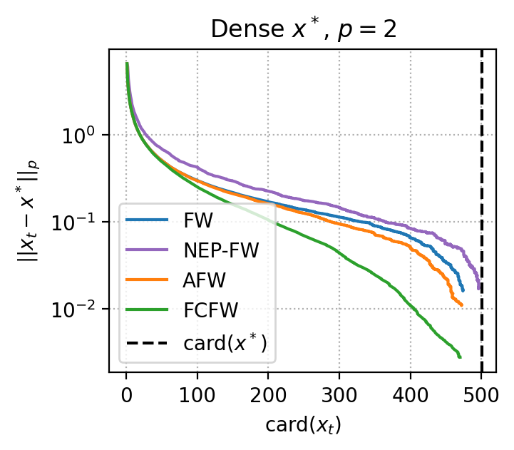
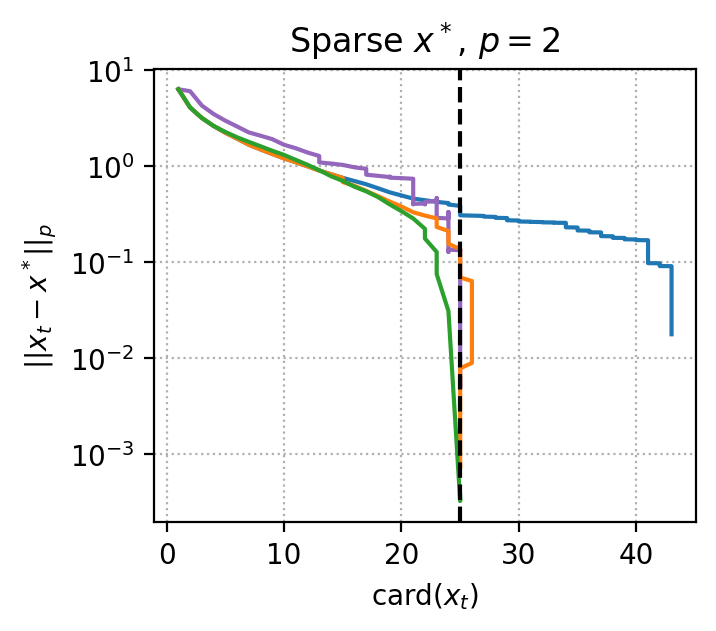
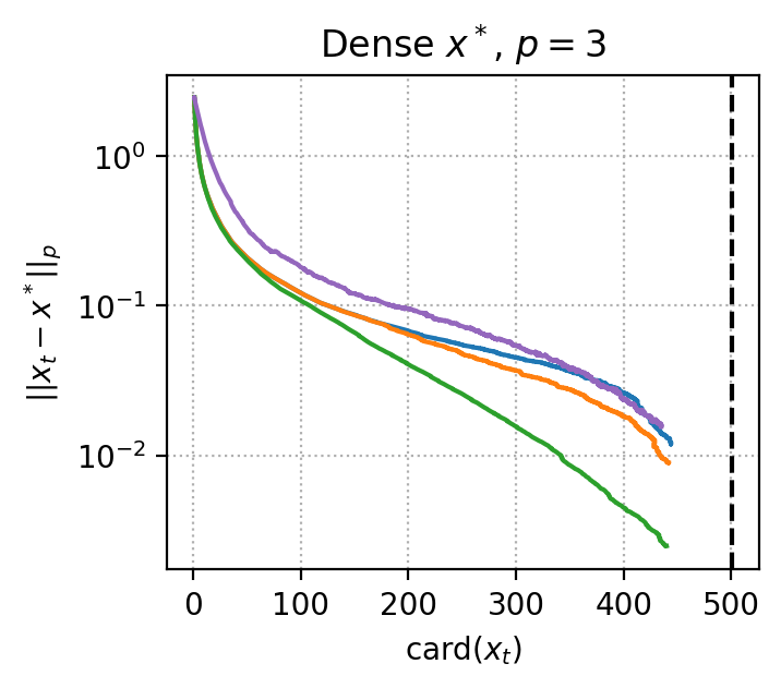
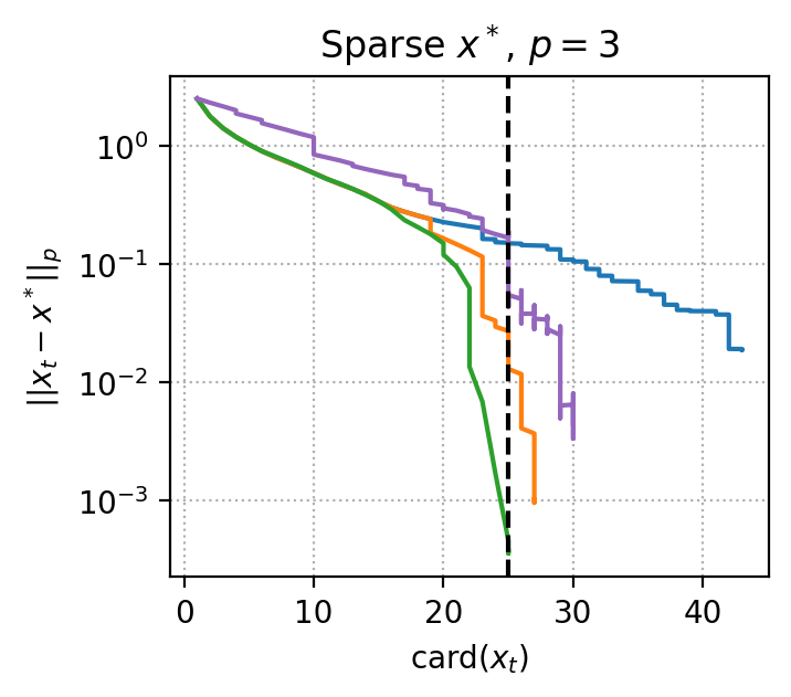
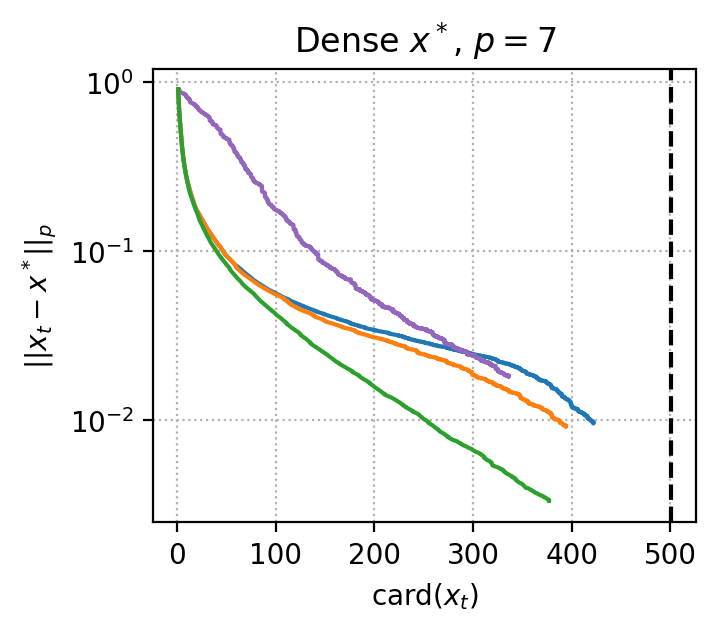
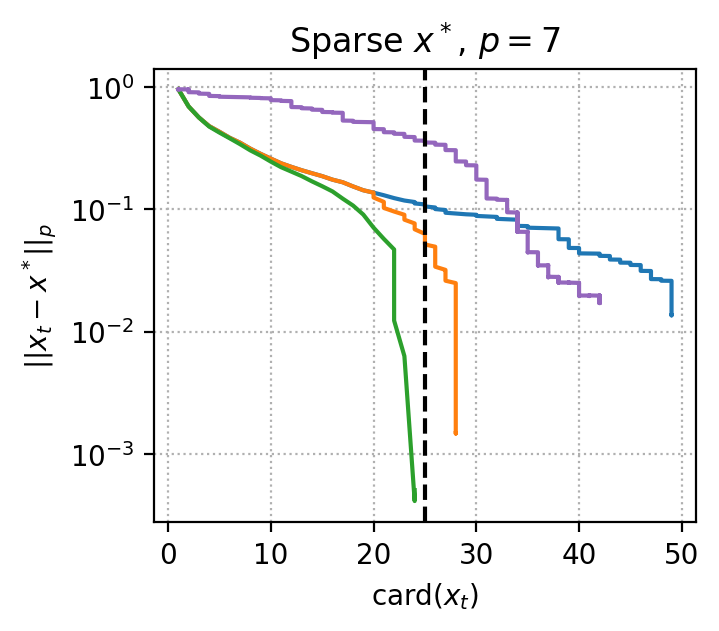
Figure 1: Accuracy vs. cardinality of the iterates generated by FW, NEP-FW, AFW, and FCFW.

As expected, FCFW is the best performing algorithm, followed by AFW. In the instance ‘‘Sparse $x^{*}$, $p=2$’’, we can see that AFW took a full away step, which decreased the cardinality of the iterate by $1$. In the limit, NEP-FW improves on FW particularly when the target $x^{*}$ is sparse; note that we chose $x_{0}\in\mathcal{V}$ randomly and did not use a warm start. Only FCFW is able to recover an optimal convex decomposition on each instance, i.e., to find a solution with arbitrary accuracy and cardinality no greater than $\operatorname{card}(x^{*})$. Table 3 reports the cardinality of the solution obtained by each algorithm to reach accuracy $\varepsilon=0.02$.

Table 3: Cardinality of the first iterate $x_{t}$ satisfying $\|x_{t}-x^{*}\|_{p}<0.02$.

$\operatorname{card}(x^{*})$	$p$	FW	NEP-FW	AFW	FCFW
$501$	$2$	$470$	$496$	$453$	$368$
$25$	$2$	$43$	$25$	$26$	$25$
$501$	$3$	$417$	$413$	$388$	$275$
$25$	$3$	$42$	$29$	$25$	$22$
$501$	$7$	$349$	$325$	$294$	$175$
$25$	$7$	$49$	$40$	$28$	$22$

8.2 Lower bound

We compare FW, AFW, and FCFW to the lower bound in [30, Sec. 5.1]. Let $\mathcal{C}$ be the convex hull of the $\ell_{p}$-normalized columns of the Hadamard matrix $H_{n}$ of dimension $n$ from Sylvester’s construction, i.e., $\mathcal{C}=\operatorname{conv}(H_{n}/n^{1/p})$, and let $x^{*}=(H_{n}/n^{1/p})1/n=e_{1}/n^{1/p}$ be the uniform convex combination of the columns, where $e_{1}\in\mathbb{R}^{n}$ denotes the first canonical vector. In this setting, [30, Thm. 5.3] claims that for any $x\in\operatorname{conv}(H_{n}/n^{1/p})$ satisfying $\|x-x^{*}\|_{p}\leqslant\varepsilon$, then $x$ has cardinality $s\geqslant\min\{1/\varepsilon^{2},n\}$. However, in their proof they use the inequality

$$\frac{1}{\varepsilon^{2}+1/n}\geqslant\frac{1}{\max\{\varepsilon^{2},1/n\}},$$

which does not hold. Hence, for completeness, we present a minor correction to their lower bound in Theorem 8.1.

Theorem 8.1.

Let $p\in\left[2,+\infty\right[$, $n\in\{2^{k}\mid k\in\mathbb{N}\}$, $H_{n}$ be the Hadamard matrix of dimension $n$ from Sylvester’s construction, $\mathcal{C}=\operatorname{conv}(H_{n}/n^{1/p})$ be the convex hull of the $\ell_{p}$-normalized columns of $H_{n}$, and $x^{*}=e_{1}/n^{1/p}\in\mathcal{C}$. Let $\varepsilon>0$ and $x\in\mathcal{C}$ such that $\|x-x^{*}\|_{p}\leqslant\varepsilon$. Then $x$ is the convex combination of at least $1/(\varepsilon^{2}+1/n)$ vertices.

Figure 2 compares FW, AFW, FCFW, and the corrected lower bound $s\in\llbracket 1,n\rrbracket\mapsto\varepsilon=\sqrt{1/s-1/n}$, for $n=64$ and two arbitrary values $p=4$ and $p=13$.

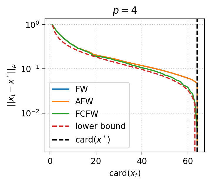
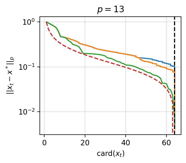
Figure 2: Cardinality of the iterates produced by FW, AFW, and FCFW, and the lower bound from Theorem 8.1.

FCFW again demonstrates its performance and almost matches the lower bound. This highlights its significance for the approximate Carathéodory problem. However, it remains an open problem to derive a precise convergence rate for FCFW, as the current analysis is transferred from the analyses of FW and AFW [25].

9 Final remarks

We have demonstrated that the Frank-Wolfe algorithm provides a simple implementation of a solution with cardinality $\mathcal{O}(pD_{p}^{2}/\varepsilon^{2})$ to the approximate Carathéodory problem in the $\ell_{p}$-norm, where $p\in\left[2,+\infty\right[$. When $x^{*}$ is in the interior of $\mathcal{C}$, which may be likely in practice, the algorithm naturally adapts and generates a solution with cardinality $\mathcal{O}(p(D_{p}/r_{p})^{2}\ln(1/\varepsilon))$, where $r_{p}$ is the radius of an ball centered at $x^{*}$ and included in $\mathcal{C}$. This is in contrast with the method in [30] which requires knowledge of $r_{p}$. The Frank-Wolfe algorithm also adapts to the geometry of $\mathcal{C}$, and generates a solution with an improved cardinality bound when $\mathcal{C}$ is uniformly convex. When $x^{*}$ is the convex combination of a subset of vertices with small diameter, better cardinality bounds are obtained via a variant of the Frank-Wolfe algorithm with an enhanced oracle. When $p\in\left[1,2\right[\cup\{+\infty\}$, new bounds are proposed via a nonsmooth variant of the algorithm. Lastly, we addressed the problem of finding sparse approximate projections in the $\ell_{p}$-norm. In practice, when $p\in\left[2,+\infty\right[$, the Fully-Corrective Frank-Wolfe algorithm is very efficient and can generate a solution with near-optimal cardinality. However, a precise estimation has yet to be derived.

Acknowledgments

Research reported in this paper was partially supported by NSF CAREER Award CMMI-1452463 and the Deutsche Forschungsgemeinschaft (DFG) through the DFG Cluster of Excellence MATH+. We thank Grigory Ivanov for providing the cardinality bound from [10, Lem. D] in the case $p\in\left]1,2\right[$ and for bringing up interesting pointers to related problems.

Appendix A Additional proofs

Lemma A.1 (Lemma 4.2).

Let Assumption 4.1 hold and consider FW (Algorithm 1) with the open-loop strategy (6) or the closed-loop strategy (4). Then

$$f(x_{1})-\min_{\mathcal{C}}f\leqslant\frac{LD^{2}}{2}.$$

Proof.

Let $x^{*}\in\operatorname*{\mathrm{arg\,min}}_{\mathcal{C}}f$ be a solution. If the open-loop strategy is used, then $\gamma_{0}=1$ so by smoothness of $f$, optimality of $v_{0}$ (Line 2), and convexity of $f$,

$$f(x_{1}) \leqslant f(x_{0})+\gamma_{0}\langle v_{0}-x_{0},\nabla f(x_{0})\rangle+\frac{L}{2}\gamma_{0}^{2}\|v_{0}-x_{0}\|^{2}$$

$$=f(x_{0})+\langle v_{0}-x_{0},\nabla f(x_{0})\rangle+\frac{L}{2}\|v_{0}-x_{0}\|^{2}$$

$$\leqslant f(x_{0})+\langle x^{*}-x_{0},\nabla f(x_{0})\rangle+\frac{LD^{2}}{2}$$

$$\leqslant f(x^{*})+\frac{LD^{2}}{2}.$$

If the closed-loop strategy is used, then by smoothness of $f$ and by optimality of the strategy (5),

$$f(x_{1}) \leqslant f(x_{0})+\gamma_{0}\langle v_{0}-x_{0},\nabla f(x_{0})\rangle+\frac{L}{2}\gamma_{0}^{2}\|v_{0}-x_{0}\|^{2}$$

$$=\min_{\gamma\in\left[0,1\right]}f(x_{0})+\gamma\langle v_{0}-x_{0},\nabla f(x_{0})\rangle+\frac{L}{2}\gamma^{2}\|v_{0}-x_{0}\|^{2}$$

$$\leqslant f(x_{0})+\langle v_{0}-x_{0},\nabla f(x_{0})\rangle+\frac{L}{2}\|v_{0}-x_{0}\|^{2},$$

and we conclude as before. ∎

Theorem A.2 (Theorem 6.4).

Let Assumption 6.1 hold and consider HCGS (Algorithm 4) with $\beta_{t}\leftarrow 2(D_{2}/G_{2})/\sqrt{t+2}$ for all $t\in\mathbb{N}$ and the open-loop strategy (6). Then for all $t\geqslant 2$,

$$f(x_{t})-\min_{\mathcal{C}}f\leqslant\frac{4G_{2}D_{2}}{\sqrt{t+1}}.$$

Proof.

Let $x^{*}\in\operatorname*{\mathrm{arg\,min}}_{\mathcal{C}}f$ and $t\in\mathbb{N}$. By Lemma 6.2, $f_{\beta_{t}}$ is convex and $1/\beta_{t}$-smooth with respect to the $\ell_{2}$-norm. By optimality of $v_{t}$ (Line 2), we have

$$f_{\beta_{t}}(x_{t+1}) \leqslant f_{\beta_{t}}(x_{t})+\gamma_{t}\langle v_{t}-x_{t},\nabla f_{\beta_{t}}(x_{t})\rangle+\frac{\gamma_{t}^{2}}{2\beta_{t}}\|v_{t}-x_{t}\|_{2}^{2}$$

$$\leqslant f_{\beta_{t}}(x_{t})+\gamma_{t}\langle x^{*}-x_{t},\nabla f_{\beta_{t}}(x_{t})\rangle+\frac{\gamma_{t}^{2}}{2\beta_{t}}\|v_{t}-x_{t}\|_{2}^{2}$$

$$\leqslant f_{\beta_{t}}(x_{t})+\gamma_{t}(f_{\beta_{t}}(x^{*})-f_{\beta_{t}}(x_{t}))+\frac{\gamma_{t}^{2}}{2\beta_{t}}\|v_{t}-x_{t}\|_{2}^{2}.$$

By [1, Lem. 4.2], $f_{\beta_{t}}(x^{*})\leqslant f(x^{*})$ and $f_{\beta_{t+1}}(x_{t+1})\leqslant f_{\beta_{t}}(x_{t+1})+(\beta_{t}-\beta_{t+1})G_{2}^{2}/2$, so

$$f_{\beta_{t+1}}(x_{t+1})-f(x^{*}) \leqslant(1-\gamma_{t})(f_{\beta_{t}}(x_{t})-f(x^{*}))+\frac{\gamma_{t}^{2}D_{2}^{2}}{2\beta_{t}}+\frac{(\beta_{t}-\beta_{t+1})G_{2}^{2}}{2}$$

$$=\frac{t}{t+2}(f_{\beta_{t}}(x_{t})-f(x^{*}))+G_{2}D_{2}\frac{\sqrt{t+2}}{(t+2)^{2}}+G_{2}D_{2}\frac{\sqrt{t+3}-\sqrt{t+2}}{\sqrt{(t+3)(t+2)}}.$$

Let $\varepsilon_{s}=f_{\beta_{s}}(x_{s})-f(x^{*})$ for all $s\in\mathbb{N}$. Then

$$(t+1)(t+2)\varepsilon_{t+1} =t(t+1)\varepsilon_{t}+G_{2}D_{2}\frac{t+1}{\sqrt{t+2}}+G_{2}D_{2}\frac{(t+1)\sqrt{t+2}}{\sqrt{t+3}}(\sqrt{t+3}-\sqrt{t+2})$$

$$\leqslant t(t+1)\varepsilon_{t}+G_{2}D_{2}\sqrt{t+2}+G_{2}D_{2}\frac{(t+1)\sqrt{t+2}}{\sqrt{t+3}}(\sqrt{t+3}-\sqrt{t+2}).$$

By telescoping for $s\in\llbracket 0,t\rrbracket$, we obtain

$$(t+1)(t+2)\varepsilon_{t+1} =G_{2}D_{2}\sum_{s=0}^{t}\sqrt{s+2}+G_{2}D_{2}\sum_{s=0}^{t}\frac{(s+1)\sqrt{s+2}}{\sqrt{s+3}}(\sqrt{s+3}-\sqrt{s+2})$$

$$\leqslant G_{2}D_{2}\sum_{s=0}^{t}\int_{s}^{s+1}\sqrt{u+2}\,\mathrm{d}u+G_{2}D_{2}\sum_{s=0}^{t}\frac{(s+1)\sqrt{s+2}}{\sqrt{s+3}}\sqrt{s+3}$$

$$\quad-G_{2}D_{2}\sum_{s=0}^{t}\frac{s\sqrt{s+1}}{\sqrt{s+2}}\sqrt{s+2}$$

$$=G_{2}D_{2}\left[\frac{2}{3}(u+2)^{3/2}\right]_{0}^{t+1}+G_{2}D_{2}\sum_{s=0}^{t}\frac{(s+1)\sqrt{s+2}}{\sqrt{s+3}}\sqrt{s+3}$$

$$\quad-G_{2}D_{2}\sum_{s=-1}^{t-1}\frac{(s+1)\sqrt{s+2}}{\sqrt{s+3}}\sqrt{s+3}$$

$$\leqslant\frac{2}{3}G_{2}D_{2}(t+3)^{3/2}+G_{2}D_{2}(t+1)\sqrt{t+2}.$$

Thus,

$$f_{\beta_{t+1}}(x_{t+1})-f(x^{*}) \leqslant\frac{2}{3}G_{2}D_{2}\frac{(t+3)^{3/2}}{(t+1)(t+2)}+\frac{G_{2}D_{2}}{\sqrt{t+2}}$$

$$\leqslant\frac{3G_{2}D_{2}}{\sqrt{t+2}},$$

where the last inequality holds for all $t\geqslant 1$. By [1, Lem. 4.2], $f(x_{t+1})\leqslant f_{\beta_{t+1}}(x_{t+1})+\beta_{t+1}G_{2}^{2}/2$. Therefore, for all $t\geqslant 1$,

$$f(x_{t+1})-f(x^{*}) \leqslant\frac{3G_{2}D_{2}}{\sqrt{t+2}}+\frac{G_{2}D_{2}}{\sqrt{t+3}}$$

$$\leqslant\frac{4G_{2}D_{2}}{\sqrt{t+2}}.$$

∎

References

- [1] A. Argyriou, M. Signoretto, and J. A. K. Suykens. Hybrid conditional gradient-smoothing algorithms with applications to sparse and low rank regularization. In Regularization, Optimization, Kernels, and Support Vector Machines, pages 53--82. Chapman & Hall/CRC, 2014.
- [2] H. Attouch, J. Bolte, P. Redont, and A. Soubeyran. Proximal alternating minimization and projection methods for nonconvex problems: An approach based on the Kurdyka-Łojasiewicz inequality. Mathematics of Operations Research, 35(2):438--457, 2010.
- [3] H. Attouch, J. Bolte, and B. F. Svaiter. Convergence of descent methods for semi-algebraic and tame problems: proximal algorithms, forward-backward splitting, and regularized Gauss-Seidel methods. Mathematical Programming, 137(1):91--129, 2013.
- [4] F. Bach. Duality between subgradient and conditional gradient methods. SIAM Journal on Optimization, 25(1):115--129, 2015.
- [5] S. Barman. Approximating Nash equilibria and dense bipartite subgraphs via an approximate version of Carathéodory’s theorem. In Proceedings of the 47th Annual ACM Symposium on Theory of Computing, pages 361--369, 2015.
- [6] H. H. Bauschke and P. L. Combettes. Convex Analysis and Monotone Operator Theory in Hilbert Spaces. Springer, 2nd edition, 2017.
- [7] J. Bolte, A. Daniilidis, A. Lewis, and M. Shiota. Clarke subgradients of stratifiable functions. SIAM Journal on Optimization, 18(2):556--572, 2007.
- [8] J. Bolte, T.-P. Nguyen, J. Peypouquet, and B. W. Suter. From error bounds to the complexity of first-order descent methods for convex functions. Mathematical Programming, 165(2):471--507, 2017.
- [9] J. Bolte, S. Sabach, and M. Teboulle. Proximal alternating linearized minimization for nonconvex and nonsmooth problems. Mathematical Programming, 146(1--2):459--494, 2014.
- [10] J. Bourgain, A. Pajor, S. J. Szarek, and N. Tomczak-Jaegermann. On the duality problem for entropy numbers of operators. In Geometric Aspects of Functional Analysis, pages 50--63. Springer, 1989.
- [11] M. D. Canon and C. D. Cullum. A tight upper bound on the rate of convergence of Frank-Wolfe algorithm. SIAM Journal on Control, 6(4):509--516, 1968.
- [12] C. Carathéodory. Über den Variabilitätsbereich der Koeffizienten von Potenzreihen, die gegebene Werte nicht annehmen. Mathematische Annalen, 64(1):95--115, 1907.
- [13] V. F. Demyanov and A. M. Rubinov. Approximate Methods in Optimization Problems. American Elsevier, 1970.
- [14] J. C. Dunn and S. Harshbarger. Conditional gradient algorithms with open loop step size rules. Journal of Mathematical Analysis and Applications, 62(2):432--444, 1978.
- [15] I. Ekeland and R. Témam. Convex Analysis and Variational Problems. Society for Industrial and Applied Mathematics, 1999. Originally published in 1976.
- [16] M. Frank and P. Wolfe. An algorithm for quadratic programming. Naval Research Logistics Quarterly, 3(1--2):95--110, 1956.
- [17] D. Garber and E. Hazan. Faster rates for the Frank-Wolfe method over strongly-convex sets. In Proceedings of the 32nd International Conference on Machine Learning, pages 541--549, 2015.
- [18] D. Garber and N. Wolf. Frank-Wolfe with a nearest extreme point oracle. In Proceedings of the 34th Conference on Learning Theory, pages 2103--2132, 2021.
- [19] J. Guélat and P. Marcotte. Some comments on Wolfe’s ‘away step’. Mathematical Programming, 35(1):110--119, 1986.
- [20] C. A. Holloway. An extension of the Frank and Wolfe method of feasible directions. Mathematical Programming, 6(1):14--27, 1974.
- [21] G. Ivanov. Approximate Carathéodory’s theorem in uniformly smooth Banach spaces. Discrete and Computational Geometry, 66(1):273--280, 2021.
- [22] M. Jaggi. Revisiting Frank-Wolfe: Projection-free sparse convex optimization. In Proceedings of the 30th International Conference on Machine Learning, pages 427--435, 2013.
- [23] T. Kerdreux, A. d’Aspremont, and S. Pokutta. Projection-free optimization on uniformly convex sets. In Proceedings of the 24th International Conference on Artificial Intelligence and Statistics, pages 19--27, 2021.
- [24] K. Kurdyka. On gradients of functions definable in o-minimal structures. Annales de l’Institut Fourier, 48(3):769--783, 1998.
- [25] S. Lacoste-Julien and M. Jaggi. On the global linear convergence of Frank-Wolfe optimization variants. In Advances in Neural Information Processing Systems, volume 28, pages 496--504, 2015.
- [26] G. Lan. The complexity of large-scale convex programming under a linear optimization oracle. Technical report, Department of Industrial and Systems Engineering, University of Florida, 2013.
- [27] E. S. Levitin and B. T. Polyak. Constrained minimization methods. USSR Computational Mathematics and Mathematical Physics, 6(5):1--50, 1966.
- [28] S. Łojasiewicz. Une propriété topologique des sous-ensembles analytiques réels. In Les Équations aux Dérivées Partielles, 117, pages 87--89. Colloques Internationaux du CNRS, 1963.
- [29] A. Maalouf, I. Jubran, and D. Feldman. Fast and accurate least-mean-squares solvers. In Advances in Neural Information Processing Systems, volume 32, pages 8307--8318, 2019.
- [30] V. Mirrokni, R. Paes Leme, A. Vladu, and S. C.-W. Wong. Tight bounds for approximate Carathéodory and beyond. In Proceedings of the 34th International Conference on Machine Learning, pages 2440--2448, 2017.
- [31] J. J. Moreau. Fonctions convexes duales et points proximaux dans un espace hilbertien. Comptes Rendus Hebdomadaires des Séances de l’Académie des Sciences, 255:2897--2899, 1962.
- [32] J. J. Moreau. Proximité et dualité dans un espace hilbertien. Bulletin de la Société Mathématique de France, 93:273--279, 1965.
- [33] A. S. Nemirovsky and D. B. Yudin. Problem Complexity and Method Efficiency in Optimization. Wiley, 1983.
- [34] G. Pisier. Remarques sur un résultat non publié de B. Maurey. In Séminaire d’Analyse Fonctionnelle, 5, pages 1--12. École Polytechnique, 1981.
- [35] B. T. Polyak. Gradient methods for the minimisation of functionals. USSR Computational Mathematics and Mathematical Physics, 3(4):864--878, 1963.
- [36] S. Shalev-Shwartz. Online Learning: Theory, Algorithms, and Applications. Ph.D. thesis, Hebrew University, 2007.
- [37] P. Wolfe. Convergence theory in nonlinear programming. In Integer and Nonlinear Programming, pages 1--36. North-Holland, 1970.
- [38] Y. Xu and T. Yang. Frank-Wolfe method is automatically adaptive to error bound condition. arXiv preprint arXiv:1810.04765, 2018.
- [39] C. Zălinescu. Convex Analysis in General Vector Spaces. World Scientific, 2002.