Casimir-Polder interactions with massive photons:
implications for BSM physics

Abstract

We present the derivation of the Casimir-Polder interactions mediated by a massive photon between two neutral systems described in terms of their atomic polarizability tensors. We find a compact expression for the leading term at large distances between the two systems. Our result reduces, in the mass-less photon limit, to the standard Casimir-Polder. We discuss implications of our findings with respect to recent scenarios of physics beyond the standard model such as universal extra dimensions, Randall-Sundrum and scale-invariant models. For each model we compute the correction to the Casimir-Polder interaction in terms of the free parameters.

I Introduction

The Casimir effect is the famous and fascinating quantum field theory phenomenon whereby two parallel plates (perfect conductors) separated a distance $a$ in vacuum attract each other with interaction energy (Casimir energy)

$${\cal E}^{C}=-\frac{\pi^{2}}{720}\frac{\hbar c}{a^{3}}$$ (1)

and it is today widely interpreted as arising from the structure of the quantum vacuum Milton (2001); Jaffe (2005); Graham et al. (2002). The interaction energy (and thus the force) between the plates is due to the difference between the vacuum energy of the electromagnetic field without and with the plates (i.e. without and with geometrical boundary conditions). Such vacuum energies, though infinite by themselves, turn out to differ by a finite amount which originates the measurable Casimir energy. In typical Casimir effect experiments Bordag et al. (2009) it is the Casimir force ${\cal P}^{C}=-\partial{\cal E}^{C}/\partial a$ that is actually measured.

It is interesting to note that historically H. B. Casimir computed initially Casimir and Polder (1948) the interaction energy between two neutral systems (atoms or molecules) at distance $r$ from each other and characterized by static polarizabilities $\alpha_{i}(0),(i=1,2)$:

$$U(r)=-\frac{1}{{{\left(4\pi\right)}}^{3}}\frac{23\,{\alpha}_{1}{\left(0\right)}{\alpha}_{2}{\left(0\right)}}{r^{7}}\,,$$ (2)

by starting with the usual van der Waals-London forces and correcting it for retardation effects. This was a standard second order perturbation theory calculation in quantum mechanics. Afterwards, apparently as a result of a conversation with Bohr Milton (2011), H. B. Casimir was able to show that the same result in Eq. (2) could be derived “studying by means of classical electrodynamics the change of the electromagnetic zero point energy” Casimir (1949). Only later Casimir (1948) he applied the same method of the vacuum fluctuations to derive the interaction energy between two perfectly conducting plates as in Eq. (1) which has become known as the Casimir effect. It is one of the most celebrated mechanical effects of vacuum fluctuations Lamoreaux (1999).

From the experimental point of view, the first convincing measurement of the Casimir effect appeared only in 1997 when it was measured Lamoreaux (1997) in the range 0.6 to 6 $\mu$m for the configuration of a plane and a sphere whose force, when the distance is small compared to the radius of the sphere, can be deduced from that for parallel plates by using the proximity force approximation. Subsequently, exact and reliable numerical calculations triggered more refined observations Mohideen and Roy (1998); Decca et al. (2005, 2007a, 2007b). For a recent review see Lamoreaux (2011). It should be remarked that essentially all previously mentioned measurements refer to the plane-sphere configuration. Indeed the measurement of the Casimir force between conductor plates is plagued with difficulties in maintaining the parallelism and by overwhelming electrostatic forces. The first precise measurement of the Casimir effect carried out in the configuration of the parallel plates was reported in Bressi et al. (2002). The first conclusive measurements of the Casimir-Polder interactions measured the force between an atom and a pair of plates in a wedge configuration Sukenik et al. (1993).

It should also be remarked that the Casimir energy and/or force in the geometry of the parallel conductors plates can be obtained via a pairwise integration of the Casimir-Polder interactions of the atoms and molecules making up the plates Milton (2001); Bordag et al. (2009).

More recently, the Casimir effect has attracted attention even in the field of superconductors. Indeed it is known that many types of superconducting detectors naturally form Casimir cavities (Superconducting Tunnel Junctions, and Transition Edge Sensor geometries) for which Casimir forces could be relevant. In these circumstances Brandt et al. (2008), since gauge invariance is broken in a superconductor, it is clear that the understanding of the Casimir effect with a massive vector field (massive photon) may become relevant. The Casimir force between two conducting lines (condensed vortices) for a massive scalar field has been investigated in de Medeiros Neto et al. (2012). In connection with these aspects, a pioneering work to address the Casimir effect between perfect conductor plates with a massive photon is that of Barton and Dombey Barton and Dombey (1984, 1985) where Proca electromagnetism Belokogne and Folacci (2016); Tu et al. (2005); Goldhaber and Nieto (2010) is used to discuss in detail the mass dependence in the limit of small photon mass. The Casimir effect with a massive vector field was then generalized to other geometries (spherical concentric) Teo (2011) and the case of real metal plates (two parallel dielectric planes) Teo (2010a, 2012) including also a discussion of temperature effects.

In the literature, several beyond the Standard Model (BSM) scenarios have been already investigated in connection with the Casimir effect in recent years. For instance within models with a generalized uncertainty principle (GUP) computing the first order correction in terms of the minimal length ($\hbar\sqrt{\beta}$) Frassino and Panella (2012); Blasone et al. (2019). Other works include investigating the Casimir effect within Randall-Sundrum models Frank et al. (2007, 2008), non commutative Randall-Sundrum models Teo (2010b), compactified universal extra dimensions (UED) Poppenhaeger et al. (2004) and a scale invariant theory (unparticles) Frassino et al. (2017). See also Frassino and Panella (2019) for an alternative approach to the unparticle Casimir effect, based on the extended problem of Caffarelli and Silvestre Caffarelli and Silvestre (2007), of the quantization of the unparticle action of a scalar field with scaling dimension $d_{\cal U}$. The Casimir effect has also been investigated in extended theories of gravity Buoninfante et al. (2019); Lambiase et al. (2017) and Post-Newtonian gravity with Lorentz-violation Blasone et al. (2018). The Casimir force for parallel plates in the spacetime with one extra space-like dimension is computed in terms of the decomposition into a Kaluza-Klein (KK) tower of massive vector fields in Teo (2010c); Edery and Marachevsky (2008).

On the other hand, one of the present authors investigated the effects of theories with a minimal length in Casimir-Polder interactions Panella (2007). To the best of our knowledge, however, the implications of theories characterized by a spectrum of massive particles have not yet been addressed in the realm of Casimir-Polder interactions. This work aims therefore at bridging such a gap by studying the Casimir-Polder interaction with a massive vector field (massive photon) and then applying the results to various BSM scenarios such as universal extra dimensions (UED), Randall-Sundrum models (RS) and scale invariant theories (unparticles).

The organization of the paper is as follows: in Sec. II we shall review the derivation of the Casimir-Polder interactions: after reviewing the Casimir-Polder within ordinary quantum electrodynamics (QED) we provide the computation of the Casimir-Polder interaction mediated by a massive vector field (massive photon). In Sec. III we discuss the Casimir-Polder energy arising within some interesting scenarios of physics beyond the standard model such as universal extra dimensions, Randall-Sundrum models and a model with scale invariance, i.e. when the interaction is mediated by an unparticle vector field. Finally Sec. V is dedicated to our conclusions.

II The Casimir-Polder interaction with a massive photon

In this section, we offer a complete derivation of the Casimir - Polder Force both for the electromagnetic field - i.e. the standard Casimir-Polder Force - and for a massive electromagnetic field.

We provide a unified approach, where the first part of the computation is valid both in the standard QED (massless) and in the massive case while in the second part we consider separately the massless and the massive results and in the end we check that the massless limit of the latter is equal to the former.

We introduce first the free electromagnetic field and then the interaction between the electromagnetic field and two non - polar molecules.

The Lagrangian density of a free vector field $A^{\mu}$ of mass $\mu$ is the Proca Lagrangian density

$$\begin{split}{\cal L}=&-\frac{1}{4}F_{\mu\nu}F^{\mu\nu}+\frac{1}{2}{\mu}^{2}A_{\mu}A^{\mu}=\\ &\frac{1}{2}A_{\mu}{\left[{\left(\Box+{\mu}^{2}\right)}{g^{\mu}}_{\nu}-{\partial}^{\mu}{\partial}_{\nu}\right]}A^{\nu}-\frac{1}{2}{\partial}_{\mu}{\left(F^{\mu\nu}A_{\nu}\right)}\end{split}$$ (3)

where

$$F^{\mu\nu}={\partial}^{\mu}A^{\nu}-{\partial}^{\nu}A^{\mu}\,,$$ (4)

and the conjugate momenta of the field $A^{\mu}(x)$ is:

$$\Pi^{\mu}(x)=F^{\mu 0}(x).$$ (5)

Then quantization of the Proca theory is carried out by imposing canonical equal time commutation relations:

$$\delta(t_{1}-t_{2})\left[A^{\mu}(x_{1}),A^{\nu}(x_{2})\right]\,=\, 0;$$ (6a)

$$\delta(t_{1}-t_{2})\left[A^{\mu}(x_{1}),\Pi^{\nu}(x_{2})\right]\,=\, i\,g^{\mu\nu}\delta^{4}(x_{1}-x_{2}).$$ (6b)

Since the Lagrangian density is defined up to a divergence it can be rewritten as

$${\cal L}=\frac{1}{2}A_{\mu}{\left[{\left(\Box+{\mu}^{2}\right)}{g^{\mu}}_{\nu}-{\partial}^{\mu}{\partial}_{\nu}\right]}A^{\nu}$$ (7)

The presence of the term in the derivatives of the second order in Eq. (7) modifies Riahi (1972) the standard EulerLagrange equations as:

$$\frac{\partial{\cal L}}{\partial A_{\mu}}-{\partial}_{\alpha}\frac{\partial{\cal L}}{\partial{\partial}_{\alpha}A_{\mu}}+{\partial}_{\alpha}{\partial}_{\beta}\frac{\partial{\cal L}}{\partial{\partial}_{\alpha}{\partial}_{\beta}A_{\mu}}=0$$ (8)

By substituting the Lagrangian density into the Euler-Lagrange equation we get the Proca equation

$${\left(\Box+{\mu}^{2}\right)}A^{\mu}-{\partial}^{\mu}{\partial}_{\nu}A^{\nu}=0\,.$$ (9)

In the massless case, the Proca equation becomes the Maxwell equation

$$\Box A^{\mu}-{\partial}^{\mu}{\partial}_{\nu}A^{\nu}=0\,.$$ (10)

In the massive case, by taking its divergence the Proca equation can be rewritten as

$$\begin{cases}{\left(\Box+{\mu}^{2}\right)}A^{\mu}=0\,,\\ {\partial}_{\mu}A^{\mu}=0\,,\end{cases}$$ (11)

where the equations are formally equal to the Klein-Gordon equation and the Lorentz Gauge, respectively. The Feynman propagator in momentum space is obtained by inverting the Fourier-transformed differential operator contained in the Lagrangian density (Greiner et al., 2013, page 188)

$$\begin{split}{{{\left(D^{-1}\right)}}^{\mu}}_{\nu}{\left(k\right)}=&-{\left(k^{2}-{\mu}^{2}\right)}{g^{\mu}}_{\nu}+k^{\mu}k_{\nu}=\\ &-{\left(k^{2}-{\mu}^{2}\right)}{\left({g^{\mu}}_{\nu}-\frac{k^{\mu}k_{\nu}}{k^{2}}\right)}+{\mu}^{2}\frac{k^{\mu}k_{\nu}}{k^{2}}\end{split}$$ (12)

Since the last expression is a spectral representation we get

$${{{\left[f{\left(D^{-1}\right)}\right]}}^{\mu}}_{\nu}{\left(k\right)} = f{\left[-{\left(k^{2}-{\mu}^{2}\right)}\right]}{\left({g^{\mu}}_{\nu}-\frac{k^{\mu}k_{\nu}}{k^{2}}\right)}$$ (13)

$$\phantom{xxxxxxxxxxx}+\,f{\left({\mu}^{2}\right)}\frac{k^{\mu}k_{\nu}}{k^{2}}$$

where $f{\left(x\right)}$ is any function. For $f{\left(x\right)}=x^{-1}$ we get

$${{D}^{\mu}}_{\nu}{\left(k\right)}=-\frac{{g^{\mu}}_{\nu}-\frac{k^{\mu}k_{\nu}}{k^{2}}}{k^{2}-{\mu}^{2}}+\frac{\frac{k^{\mu}k_{\nu}}{k^{2}}}{{\mu}^{2}}=-\frac{{g^{\mu}}_{\nu}-\frac{k^{\mu}k_{\nu}}{{\mu}^{2}}}{k^{2}-{\mu}^{2}}$$ (14)

and the Feynman propagator in momentum space is therefore

$$D^{\mu\nu}{\left(k\right)}=\frac{-g^{\mu\nu}+\frac{k^{\mu}k^{\nu}}{{\mu}^{2}}}{k^{2}-{\mu}^{2}+i0^{{}^{+}}}\,,$$ (15)

where the pole is shifted as usual by adding a small negative imaginary part to the mass in order to satisfy the causality condition (Greiner et al., 2013, page 188). The Feynman propagator in position space is obtained by Fourier anti-transforming:

$$D^{\mu\nu}{\left(x\right)}={\left(-g^{\mu\nu}-\frac{{\partial}^{\mu}{\partial}^{\nu}}{{\mu}^{2}}\right)}\int\frac{d^{4}k}{(2\pi)^{4}}\frac{e^{-ikx}}{k^{2}-{\mu}^{2}+i0^{{}^{+}}}\,.$$ (16)

The appearance of a divergent term as $\mu\to 0$ could lead to the naive conclusion that it is not possible to recover standard quantum electrodynamics, by taking the mass-less limit of the Proca theory. However, gauge invariance will save the day. Computation of physical observables will involve gauge invariant quantities like for instance the correlation functions of the field strength tensor components (electric and/or magnetic fields). These correlations functions will have a finite $\mu\to 0$ limit. Indeed by making use of the equal time commutation relations given in Eqs. (6a,6b) the following identity can be proved:

$$\begin{split}\expectationvalue{T{\left[F^{\alpha\beta}{\left(x_{1}\right)}F^{\gamma 0}{\left(x_{2}\right)}\right]}}{0}&=+{\left({{\partial}_{1}}^{\alpha}{g^{\beta}}_{\mu}-{{\partial}_{1}}^{\beta}{g^{\alpha}}_{\mu}\right)}{\left({{\partial}_{2}}^{\gamma}{g^{0}}_{\nu}-{{\partial}_{2}}^{0}{g^{\gamma}}_{\nu}\right)}\expectationvalue{T{\left[A^{\mu}{\left(x_{1}\right)}A^{\nu}{\left(x_{2}\right)}\right]}}{0}\\ &\phantom{=}-i(g^{\alpha}_{\phantom{\alpha}0}g^{\beta\gamma}-g^{\beta}_{\phantom{\beta}0}g^{\alpha\gamma})\delta^{4}(x_{1}-x_{2})\end{split}$$ (17a)

$$\begin{split}&=+i{\left({{\partial}_{1}}^{\alpha}{g^{\beta}}_{\mu}-{{\partial}_{1}}^{\beta}{g^{\alpha}}_{\mu}\right)}{\left({{\partial}_{2}}^{\gamma}{g^{0}}_{\nu}-{{\partial}_{2}}^{0}{g^{\gamma}}_{\nu}\right)}D^{\mu\nu}{\left(x_{1}-x_{2}\right)}\\ &\phantom{=}-i(g^{\alpha}_{\phantom{\alpha}0}g^{\beta\gamma}-g^{\beta}_{\phantom{\beta}0}g^{\alpha\gamma})\delta^{4}(x_{1}-x_{2})\end{split}$$ (17b)

$$\begin{split}&=+i{\left({\partial}^{\alpha}{g^{\beta}}_{\mu}-{\partial}^{\beta}{g^{\alpha}}_{\mu}\right)}{\left(-{\partial}^{\gamma}{g^{0}}_{\nu}+{\partial}^{0}{g^{\gamma}}_{\nu}\right)}{\left(-g^{\mu\nu}-\frac{{\partial}^{\mu}{\partial}^{\nu}}{{\mu}^{2}}\right)}\int\frac{d^{4}k}{(2\pi)^{4}}\frac{e^{-ik{\left(x_{1}-x_{2}\right)}}}{k^{2}-{\mu}^{2}+i0^{{}^{+}}}\\ &\phantom{=}-i(g^{\alpha}_{\phantom{\alpha}0}g^{\beta\gamma}-g^{\beta}_{\phantom{\beta}0}g^{\alpha\gamma})\delta^{4}(x_{1}-x_{2})\end{split}$$ (17c)

$$\begin{split}&=+i{\left({\partial}^{\alpha}{g^{\beta}}_{\mu}-{\partial}^{\beta}{g^{\alpha}}_{\mu}\right)}{\left({\partial}^{\gamma}g^{0\mu}-{\partial}^{0}g^{\gamma\mu}\right)}\int\frac{d^{4}k}{(2\pi)^{4}}\frac{e^{-ik{\left(x_{1}-x_{2}\right)}}}{k^{2}-{\mu}^{2}+i0^{{}^{+}}}\\ &\phantom{=}-i(g^{\alpha}_{\phantom{\alpha}0}g^{\beta\gamma}-g^{\beta}_{\phantom{\beta}0}g^{\alpha\gamma})\delta^{4}(x_{1}-x_{2})\,.\end{split}$$ (17d)

It can be seen that the divergent terms cancel out each other in Eq. (LABEL:BraketTensorC) and the above correlations admit indeed a well defined massless limit $\mu\to 0$.

The interaction Hamiltonian between the electromagnetic field and the neutral systems (atomes/molecules) placed at the positions $\bm{r}_{1}$ and $\bm{r}_{2}$ (with $\bm{r}_{2}\neq\bm{r}_{1}$) is the dipole interaction:

$$H_{int}{\left(t\right)}=-\bm{E}{\left(t,{\bm{r}}_{1}\right)}\cdot{\bm{d}}_{(1)}{\left(t\right)}-\bm{E}{\left(t,{\bm{r}}_{2}\right)}\cdot{\bm{d}}_{(2)}{\left(t\right)}$$ (18)

where $\bm{E}{\left(t,\bm{r}\right)}$ is the electric field operator, ${\bm{r}}_{k}$ is the position and ${\bm{d}}_{(k)}$ is the electric dipole moment operator of the $k^{th}$ atom/molecule $(k=1,2)$.

Since the neutral atoms/molecules are assumed to be non-polar $\expectationvalue{{\bm{d}_{(k)}}}{{\psi}}=0$ the potential energy from second order perturbation theory (Berestetskii et al., 2012, page 348) vanishes.

The first non vanishing contribution to the potential energy comes then from fourth order perturbation theory (Berestetskii et al., 2012, page 348)

$$U{\left(\mu;{\bm{r}}_{1},{\bm{r}}_{2}\right)} = \frac{i}{2t}\int dt_{1}dt_{2}dt_{3}dt_{4}\,\times$$ (19)

$$\expectationvalue{T{\left[E^{i}{\left(t_{1},{\bm{r}}_{1}\right)}E^{j}{\left(t_{2},{\bm{r}}_{2}\right)}\right]}}{0}\times$$

$$\expectationvalue{T{\left[{d_{2}}^{j}{\left(t_{2}\right)}{d_{2}}^{l}{\left(t_{4}\right)}\right]}}{{\psi}_{2}}\times$$

$$\expectationvalue{T{\left[E^{l}{\left(t_{4},{\bm{r}}_{2}\right)}E^{k}{\left(t_{3},{\bm{r}}_{1}\right)}\right]}}{0}\times$$

$$\expectationvalue{T{\left[{d_{1}}^{k}{\left(t_{3}\right)}{d_{1}}^{i}{\left(t_{1}\right)}\right]}}{{\psi}_{1}}$$

which in the language of Feynman diagrams is represented by a loop diagram with a two photon exchange.

When computing the correlation function $\langle 0|T\left[E^{i}{\left(t_{1},{\bm{r}}_{1}\right)}E^{j}{\left(t_{2},{\bm{r}}_{2}\right)}\right]|0\rangle$ the commutation of the time derivatives which enter the electric fields $E^{i}$ with the chronological $T-$product introduces terms proportional to $\delta^{4}(x_{1}-x_{2})=\delta(t_{1}-t_{2})\,\delta^{3}(\bm{r}_{1}-\bm{r}_{2})$, as can be seen from Eq. (17a). Since we are interested in the interaction energy between the two systems located at $\bm{r}_{1},\bm{r}_{2}$ with $\bm{r}_{1}\neq\bm{r}_{2}$, clearly $\delta^{3}(\bm{r}_{1}-\bm{r}_{2})=0$. Such terms proportional to the Dirac distribution $\delta^{4}(x_{1}-x_{2})$ can be safely ignored and we conclude that time derivatives can be taken out of the $T-$product like the corresponding spatial derivatives. Therefore from Eq. (LABEL:BraketTensorD) we get:

$$\langle 0| T\left[E^{i}{\left(t_{1},{\bm{r}}_{1}\right)}E^{j}{\left(t_{2},{\bm{r}}_{2}\right)}\right]|0\rangle$$

$$=\expectationvalue{T{\left[F^{i0}{\left(t_{1},{\bm{r}}_{1}\right)}F^{j0}{\left(t_{2},{\bm{r}}_{2}\right)}\right]}}{0}$$

$$=i{\left({\partial}^{i}{\partial}^{j}-{\partial}^{0}{\partial}^{0}{\delta}^{ij}\right)}\!\!\int\limits_{-\infty}^{\infty}\!\!\frac{d\omega}{2\pi}D{\left(\omega,{\bm{r}}_{1}\!-\!{\bm{r}}_{2}\right)}e^{-i\omega{\left(t_{1}-t_{2}\right)}}$$

$$=i\int\limits_{-\infty}^{\infty}\frac{d\omega}{2\pi}{\left({\omega}^{2}{\delta}^{ij}+{\partial}^{i}{\partial}^{j}\right)}D{\left(\omega,{\bm{r}}_{1}\!-\!{\bm{r}}_{2}\right)}e^{-i\omega{\left(t_{1}-t_{2}\right)}}$$

where we have defined the scalar function $D{\left(\omega,\bm{r}\right)}$ as:

$$D{\left(\omega,\bm{r}\right)}=\int\frac{d^{3}\bm{k}}{{{\left(2\pi\right)}}^{3}}\,\frac{e^{i\bm{k}\cdot\bm{r}}}{k^{2}-{\mu}^{2}+i0^{{}^{+}}}\,.$$ (21)

It can be shown that (Berestetskii et al., 2012, page 351)

$$\expectationvalue{T{\left[{d_{k}}^{i}{\left(t_{1}\right)}{d_{k}}^{j}{\left(t_{2}\right)}\right]}}{{\psi}_{k}}=i\int\limits_{-\infty}^{\infty}\frac{d\omega}{2\pi}\alpha_{k}^{ij}{\left(\omega\right)}e^{-i\omega{\left(t_{1}-t_{2}\right)}}$$ (22)

where ${{\alpha}_{k}}^{ij}$ is the polarizability tensor of the $k^{th}$ molecule and ${{\alpha}_{k}}^{ij}{\left(-\omega\right)}={{\alpha}_{k}}^{ij}{\left(\omega\right)}$. By substituting Eq. (II) and (22) in Eq. (19) and recognizing the Dirac delta functions we get:

$$U{\left(\mu{;}\,{\bm{r}}_{1}{-}{\bm{r}}_{2}\right)}{=}\frac{1}{4\pi}i{\int_{{-}\infty}^{\infty}}{\left[{\left({\omega}^{2}{\delta}^{ij}{+}{\partial}^{i}{\partial}^{j}\right)}D{\left(\omega{,}{\bm{r}}_{1}{-}{\bm{r}}_{2}\right)}\right]}{{\alpha}_{2}}^{jl}{\left(\omega\right)}{\left[{\left({\omega}^{2}{\delta}^{lk}{+}{\partial}^{l}{\partial}^{k}\right)}D{\left(\omega{,}{\bm{r}}_{2}{-}{\bm{r}}_{1}\right)}\right]}{{\alpha}_{1}}^{ki}{\left(\omega\right)}d\omega$$ (23)

We readily recognize a trace in the expression above

$$U{\left(\mu;\,{\bm{r}}_{1}-{\bm{r}}_{2}\right)}=\frac{1}{4\pi}i\int_{-\infty}^{\infty}\text{Tr}\,{\left[{\left({\omega}^{2}\mathbb{1}+\mathbb{H}\right)}D{\left(\omega,{\bm{r}}_{1}-{\bm{r}}_{2}\right)}\right]}{\mathbb{a}}_{2}{\left(\omega\right)}{\left[{\left({\omega}^{2}\mathbb{1}+\mathbb{H}\right)}D{\left(\omega,{\bm{r}}_{2}-{\bm{r}}_{1}\right)}\right]}{\mathbb{a}}_{1}{\left(\omega\right)}d\omega$$ (24)

where $\mathbb{H}=\partial^{i}\partial^{j}$ is the Hessian matrix, $\mathbb{1}=\delta^{ij}$ is the identity operator and $\mathbb{a}_{k}=\alpha_{k}^{ij}(k=1,2)$ are the polarization tensors of the two neutral systems.

By using the facts that $D{\left(-\omega,\bm{r}\right)}=D{\left(\omega,\bm{r}\right)}$ and ${\mathbb{a}}_{k}{\left(-\omega\right)}={\mathbb{a}}_{k}{\left(\omega\right)}$ we get:

$$U\left(\mu;{\bm{r}}_{1}-{\bm{r}}_{2}\right) = i\int_{0}^{\infty}\frac{d\omega}{2\pi}\,\text{Tr}\left[\left(\omega^{2}\mathbb{1}+\mathbb{H}\right)D\left(\omega,\bm{r}_{1}-\bm{r}_{2}\right)\right.$$

$$\left.\times\mathbb{a}_{2}\left(\omega\right)\left(\omega^{2}\mathbb{1}+\mathbb{H}\right)D{\left(\omega,{\bm{r}}_{2}-{\bm{r}}_{1}\right)}\right]\mathbb{a}_{1}(\omega)$$

By using the fact that $D{\left(\omega,\bm{r}\right)}=D{\left(\omega,{\left|\bm{r}\right|}\right)}$ and considering the case of isotropic molecules $\alpha_{k}^{ij}(\omega)=\alpha_{k}(\omega)\delta^{ij}$  follows

$$U{\left(\mu;r\right)}=i\int_{0}^{\infty}\frac{d\omega}{2\pi}{\alpha}_{1}{\left(\omega\right)}{\alpha}_{2}{\left(\omega\right)}\,\text{Tr}\,{{\left[{\left({\omega}^{2}\mathbb{1}+\mathbb{H}\right)}D{\left(\omega,r\right)}\right]}}^{2}$$ (26)

where $r={\left|{\bm{r}}_{1}-{\bm{r}}_{2}\right|}$. By expanding ${\alpha}_{k}{\left(\omega\right)}$ we can compute ${\alpha}_{1}{\left(\omega\right)}{\alpha}_{2}{\left(\omega\right)}$ as a product of two series (Cauchy product), and by using again ${\alpha}_{k}{\left(-\omega\right)}={\alpha}_{k}{\left(\omega\right)}$ we get the following series

$${\alpha}_{1}{\left(\omega\right)}{\alpha}_{2}{\left(\omega\right)} = \sum_{n=0}^{\infty}\frac{{\omega}^{2n}}{{\left(2n\right)}!}\times$$

$$\sum_{k=0}^{n}\binom{2n}{2k}\frac{d^{2k}{\alpha}_{1}}{d{\omega}^{2k}}{\left(0\right)}\frac{d^{2(n-k)}{\alpha}_{2}}{d{\omega}^{2(n-k)}}{\left(0\right)},$$

and by using the fact that the Laplacian is the trace of the Hessian matrix it follows:

$$\text{Tr}[(\omega^{2}\mathbb{1} + \mathbb{H})D(\omega r)]^{2}=3{\omega}^{4}D^{2}{\left(\omega,r\right)}$$

$$+2{\omega}^{2}D{\left(\omega,r\right)}{\nabla}^{2}D{\left(\omega,r\right)}+\text{Tr}{\left\{{{\left[\mathbb{H}D{\left(\omega,r\right)}\right]}}^{2}\right\}}$$

and in spherical coordinates:

$$\mathbb{H}D{\left(\omega r\right)}=\frac{1}{r}\frac{\partial D}{\partial r}{\left(\omega r\right)}{\left(\mathbb{1}-\frac{xx^{T}}{r^{2}}\right)}+\frac{{\partial}^{2}D}{\partial r^{2}}{\left(\omega,r\right)}\frac{xx^{T}}{r^{2}}$$ (29)

where $\mathbb{1}$ is the identity matrix, $x$ is the position column vector, ${x}^{T}$ denotes the transposed position vector and, of course, we have used only the radial term of the Hessian matrix. Since this is a spectral representation one can write:

$$f{\left[\mathbb{H}D{\left(\omega,r\right)}\right]} = f{\left[\frac{1}{r}\frac{\partial D}{\partial r}{\left(\omega,r\right)}\right]}{\left(\mathbb{1}-\frac{xx^{T}}{r^{2}}\right)}$$ (30)

$$\phantom{xxxx}+f{\left[\frac{{\partial}^{2}D}{\partial r^{2}}{\left(\omega,r\right)}\right]}\frac{xx^{T}}{r^{2}}$$

where $f{\left(x\right)}$ is a function. And, since we need to compute Tr${\left[\mathbb{H}D{\left(\omega,r\right)}\right]^{2}}$ in Eq. (II), for $f{\left(x\right)}=x^{2}$, the previous Eq. (30) is:

$${{\left[\mathbb{H}D{\left(\omega,r\right)}\right]}}^{2} = {{\left[\frac{1}{r}\frac{\partial D}{\partial r}{\left(\omega,r\right)}\right]}}^{2}{\left(\mathbb{1}-\frac{xx^{T}}{r^{2}}\right)}$$ (31)

$$\phantom{xxxx}+{{\left[\frac{{\partial}^{2}D}{\partial r^{2}}{\left(\omega,r\right)}\right]}}^{2}\frac{xx^{T}}{r^{2}}.$$

The computation of the trace

$$\text{Tr}{{\left[\mathbb{H}D{\left(\omega,r\right)}\right]}}^{2}=2{{\left[\frac{1}{r}\frac{\partial D}{\partial r}{\left(\omega,r\right)}\right]}}^{2}+{{\left[\frac{{\partial}^{2}D}{\partial r^{2}}{\left(\omega,r\right)}\right]}}^{2}$$ (32)

finally gives:

$$\text{Tr}{{\left[{\left({\omega}^{2}\mathbb{1}{+}\mathbb{H}\right)}D{\left(\omega{,}r\right)}\right]}}^{2} = \,3\,{\omega}^{4}D^{2}{\left(\omega{,}r\right)}$$

$${+} \,2{\omega}^{2}D{\left(\omega{,}r\right)}\frac{1}{r^{2}}\frac{\partial}{\partial r}r^{2}\frac{\partial D}{\partial r}{\left(\omega{,}r\right)}$$

$${+} \,2{{\left[\frac{1}{r}\frac{\partial D}{\partial r}{\left(\omega{,}r\right)}\right]}}^{2}{+}{{\left[\frac{{\partial}^{2}D}{\partial r^{2}}{\left(\omega{,}r\right)}\right]}}^{2}.$$

By substituting Eq. (II) and Eq. (II) in Eq. (26) we obtain the explicit expression for the potential energy:

$$U\left(\mu;r\right) = \,i\sum_{n=0}^{\infty}\int_{0}^{\infty}\frac{d\omega}{2\pi}\,\frac{{\omega}^{2n}}{{\left(2n\right)}!}\,\left\{3\omega^{4}D^{2}\left(\omega{,}r\right)\phantom{\left[\frac{1}{r}\right]^{2}}\right.$$ (34)

$$\,+2\omega^{2}D\left(\omega{,}r\right)\frac{1}{r^{2}}\frac{\partial}{\partial r}r^{2}\frac{\partial D}{\partial r}\left(\omega{,}r\right)$$

$${+}\left.2{{\left[\frac{1}{r}\frac{\partial D}{\partial r}{\left(\omega{,}r\right)}\right]}}^{2}+{{\left[\frac{{\partial}^{2}D}{\partial r^{2}}{\left(\omega{,}r\right)}\right]}}^{2}\right\}\times$$

$$\sum_{k=0}^{n}\binom{2n}{2k}\frac{d^{2k}{\alpha}_{1}}{d{\omega}^{2k}}{\left(0\right)}\frac{d^{2n-2k}{\alpha}_{2}}{d{\omega}^{2n-2k}}{\left(0\right)}.$$

This will be the starting point for our analysis in the next subsections.

II.1 Casimir-Polder interaction for massless photons

The scalar function $D(\omega,\bm{r})$ defined in Eq. (21) in the massless photon case (when $\mu=0)$ is easily computed by using standard methods as:

$$D{\left(\omega,r\right)}=\int\!\!\frac{d^{3}\bm{k}}{(2\pi)^{3}}\,\frac{e^{i\bm{k}\cdot\bm{r}}}{k^{2}+i0^{{}^{+}}}=-\frac{1}{4\pi}\frac{e^{i{\left|\omega\right|}r}}{r}$$ (35)

By substituting Eq. (35) in Eq. (34) and differentiating

$$U{\left(\mu{=}0{;}r\right)}{=} \frac{4i}{(4\pi)^{3}\,r^{6}}{\sum_{n{=}0}^{\infty}}{\int_{0}^{\infty}}\,d\omega\,{g}_{0}{\left({-}i\omega r\right)}{{\left(2\omega r\right)}}^{2n}\times$$ (36)

$$e^{2i\omega{\left(r{+}i0^{+}\right)}}\,\left(\frac{1}{2r}\right)^{2n}\,\frac{1}{\left(2n\right)!}\times$$

$${\sum_{k{=}0}^{n}}\binom{2n}{2k}\frac{d^{2k}{\alpha}_{1}}{d{\omega}^{2k}}{\left(0\right)}\frac{d^{2n{-}2k}{\alpha}_{2}}{d{\omega}^{2n{-}2k}}{\left(0\right)}$$

where

$${g}_{0}{\left(x\right)}=x^{4}+2x^{3}+5x^{2}+6x+3,$$ (37)

and we have regularized the integral.
Changing the variable $x=2\omega r$ in Eq. (36)

$$U{\left(\mu{=}0{;}r\right)}{=} \frac{1}{{{\left(4\pi\right)}}^{3}}\frac{2i}{r^{7}}\sum_{n{=}0}^{\infty}\int_{0}^{\infty}\,dx\,{g}_{0}{\left({-}i\frac{x}{2}\right)}x^{2n}e^{ix{\left(1{+}i0^{+}\right)}}$$

$$\times\frac{{{\left(\frac{1}{2r}\right)}}^{2n}}{{\left(2n\right)}!}\sum_{k{=}0}^{n}\binom{2n}{2k}\frac{d^{2k}{\alpha}_{1}}{d{\omega}^{2k}}{\left(0\right)}\frac{d^{2n{-}2k}{\alpha}_{2}}{d{\omega}^{2n{-}2k}}{\left(0\right)}$$

and using the formula

$$\int_{0}^{\infty}x^{n}e^{ix{\left(1{+}i0^{+}\right)}}dx=i^{n+1}n!$$ (39)

we get the final result:

$$U{\left(\mu{=}0{;}r\right)}{=} {-}\frac{1}{{{\left(4\pi\right)}}^{3}}\frac{1}{r^{7}}{\sum_{n{=}0}^{\infty}}\frac{{\left(4n^{2}{+}16n{+}23\right)}{\left(n{+}2\right)}{\left(n{+}1\right)}}{2}$$

$$\times{{\left({-}\frac{1}{4r^{2}}\right)}}^{n}{\sum_{k{=}0}^{n}}\binom{2n}{2k}\frac{d^{2k}{\alpha}_{1}}{d{\omega}^{2k}}{\left(0\right)}\frac{d^{2n{-}2k}{\alpha}_{2}}{d{\omega}^{2n{-}2k}}{\left(0\right)}.$$

The leading term of the series is the well known Casimir-Polder potential energy between two neutral atomic systems with static polarizability $\alpha_{1,2}(0)$ given in Eq. (2).

II.2 Casimir - Polder interaction for massive photons

By using standard mathematical procedures (Jordan’s lemma and Cauchy’s residue theorem) we get from Eq. (21) in the case $\mu\neq 0$:

$$D{\left(\omega,r\right)}=-\frac{1}{4\pi r}\begin{cases}e^{-\sqrt{{\mu}^{2}-{\omega}^{2}}r}&{\left({\left|\omega\right|}\leq\mu\right)}\\ e^{i\sqrt{{\omega}^{2}-{\mu}^{2}}r}&{\left({\left|\omega\right|}\geq\mu\right)}\end{cases}$$ (41)

By substituting (41) in (34), differentiating and performing the appropriate change of variables one obtains the following expression:

$$U{\left(\mu;r\right)}=U_{1}{\left(\mu;r\right)}+U_{2}{\left(\mu;r\right)}$$ (42)

$$U_{1}\left(\mu;r\right) = -\frac{1}{{{\left(4\pi\right)}}^{3}}\frac{1}{r^{7}}\sum_{n=0}^{\infty}\int_{0}^{2\mu r}\frac{xdx}{2}{{\left[{{\left(2\mu r\right)}}^{2}-x^{2}\right]}}^{n-\frac{1}{2}}\times$$ (43)

$${g}_{\mu}{\left(\frac{x}{2}\right)}e^{-x}\,\left(\frac{1}{2r}\right)^{2n}\,\frac{1}{\left(2n\right)!}\times$$

$$\sum_{k=0}^{n}\binom{2n}{2k}\frac{d^{2k}{\alpha}_{1}}{d{\omega}^{2k}}{\left(0\right)}\frac{d^{2n-2k}{\alpha}_{2}}{d{\omega}^{2n-2k}}{\left(0\right)}$$

$$U_{2}{\left(\mu;r\right)} = -\frac{1}{{{\left(4\pi\right)}}^{3}}\frac{1}{r^{7}}\sum_{n=0}^{\infty}\int_{0}^{\infty}\frac{xdx}{2}{{\left[{{\left(2\mu r\right)}}^{2}+x^{2}\right]}}^{n-\frac{1}{2}}\times$$ (44)

$${g}_{\mu}{\left(-i\frac{x}{2}\right)}e^{ix{\left(1+i0^{+}\right)}}\,\left(\frac{1}{2r}\right)^{2n}\,\frac{1}{\left(2n\right)!}\times$$

$$\sum_{k=0}^{n}\binom{2n}{2k}\frac{d^{2k}{\alpha}_{1}}{d{\omega}^{2k}}{\left(0\right)}\frac{d^{2n-2k}{\alpha}_{2}}{d{\omega}^{2n-2k}}{\left(0\right)},$$

where in this case (both in Eq. (43) and Eq. (44)):

$${g}_{\mu}{\left(x\right)}=$$

$$\frac{2}{i}{\left[3{{\left(\mu r\right)}}^{4}-4{{\left(\mu r\right)}}^{2}x^{2}+2{\left(x^{4}+2x^{3}+5x^{2}+6x+3\right)}\right]}$$

and we have regularized the integral in Eq. (44). Therefore, for the massive case, the final result reads

$$U{\left(\mu;r\right)}= -\frac{1}{{{\left(4\pi\right)}}^{3}}\frac{1}{r^{7}}\sum_{n=0}^{\infty}\left[2K_{n+1}{\left(2\mu r\right)}{{\left(\mu r\right)}}^{n+5}\right.$$

$${+}8K_{n+2}{\left(2\mu r\right)}{{\left(\mu r\right)}}^{n+4}$$

$$\left.{+}{\left(4n^{2}{+}16n{+}23\right)}K_{n+3}{\left(2\mu r\right)}{{\left(\mu r\right)}}^{n+3}\right]$$

$$\times\frac{{{\left(-\frac{1}{4r^{2}}\right)}}^{n}}{n!}\sum_{k=0}^{n}\binom{2n}{2k}\frac{d^{2k}{\alpha}_{1}}{d{\omega}^{2k}}{\left(0\right)}\frac{d^{2n-2k}{\alpha}_{2}}{d{\omega}^{2n-2k}}{\left(0\right)}$$

where $K_{n}{\left(x\right)}$ is the modified Bessel function of the second kind. Performing the limit $\mu\rightarrow 0$:

$$\lim_{x\to 0^{{}^{+}}}K_{n}{\left(2x\right)}x^{n}=\frac{{\left(n-1\right)}!}{2}$$ (47)

we see that in the massless limit of Eq. (II.2) we recover the series in Eq. (II.1). The first (dominant) term in the above series (II.2) is:

$$U\left(\mu\right. \left.r\right)=-\frac{1}{\left(4\pi\right)^{3}}\frac{\alpha_{1}(0)\,\alpha_{2}(0)}{r^{7}}\left[2\,K_{1}(2\mu r)(\mu r)^{5}\right.$$ ; (48)

$$+\left.8\,K_{2}(2\mu r)(\mu r)^{4}+23\,K_{3}(2\mu r)(\mu r)^{3}\right].$$

And of course in the limit $\mu\to 0$ from Eq. (48) we readily recover the standard QED Casimir-Polder result, i.e. Eq. (2). We emphasize that Eq. (II.2) and Eq. (48) are the central results of the present work. In the following, we will use mainly Eq. (48) (the leading term) to address some beyond the standard model scenarios with respect to the Casimir-Polder interactions.

III Casimir-polder interaction in BSM models

In this section we discuss the Casimir-polder interactions in a number of alternative scenarios of physics beyond the standard model (BSM). Specifically, we consider: (A) universal extra dimensions, (B) Randall Sundrum models and (C) scale-invariant models. For each of the above BSM scenarios, the standard Casimir effect has been already discussed in the literature (see references in the introduction and in the following sections).

III.1 Universal Extra Dimensions (UED)

In the UED scenario Fabiano and Panella (2010), all standard model fields are assumed to propagate in a bulk space-time with extra space-like dimensions compactified to a circle of radius $R$. Upon quantization of the (4+D) dimensional theory the effect of the extra dimension(s) is, for a given standard model field $X$, that there is a tower of Kaluza-Klein states $X_{n}$, $n=1,2,\dots$ with masses:

$$m^{2}_{n}=m^{2}_{0}+\frac{n^{2}}{R^{2}}$$ (49)

where $m_{0}$ is the mass of the lowest lying state $X_{0}$. For the photon $m_{0}=0$ and thus the photon is then accompained by a Kaluza-Klein tower (KK-tower) of massive photons $\gamma_{n}$ of mass $m_{n}=n/R$. Recent bounds on the size of the extra dimensions come from the non observation of Kaluza-Klein excitations at Tevatron and are already quite stringent: $R\leq 300\,\,\text{GeV}^{-1}\approx 10^{-9}\,\,\text{nm}$ Appelquist et al. (2001); Macesanu et al. (2002); Rizzo (2001). Stronger bounds are of course now available from LHC experiments and typical ATLAS Aad et al. (2015) and CMS analyses exclude now values of $R^{-1}$ smaller than $\sim(1\,\text{TeV})^{-1}$ Beuria et al. (2018) (or equivalently the allowed values of $R$ are those such that $R\leq\text{1\ TeV}^{-1}\approx 0.3\times 10^{-9}\text{nm}$). Interestingly, considerations from the relic density in the UED model assuming $\gamma_{1}$ to be the lightest Kaluza-Klein particle (LKP) give a preferred range for the size of the extra dimension: $R^{-1}\sim 1.3-1.5$ TeV Bélanger et al. (2011) thus providing also an upper bound for $R^{-1}$ (or a lower bound for $R$).

The Casimir effect in the geometry of parallel conductor plates within UED has been addressed in Poppenhaeger et al. (2004); Pascoal et al. (2008), and the bounds that can be obtained are quite less stringent: $R<10$ nm Poppenhaeger et al. (2004). Given that typical current state of the art Casimir/Casimir-Polder experiments can probe distances ($r$) down to the nanometer range if we assume the more stringent high energy bound on the compactification size $R$ of the extra dimension ($R\approx 0.3\times 10^{-9}$ nm) the quantity $\xi=r/R$ is a very large quantity $\xi\approx 10^{10}$. Clearly for each one of the Kaluza-Klein massive photons $\gamma_{n}$ we can compute its contribution to the Casimir-Polder interaction of the two neutral systems via the result obtained in the previous section for the massive photon case in Eq. (II.2). In particular let us consider only the dominant term in the series in Eq. (II.2), that is the approximation in Eq. (48). We can then estimate the total KK-tower contribution as summing, for every mass eigen-state, a term given by Eq. (48):

$$U_{\text{KK}} \!\!\!\!\!\!\!(r,R)=\sum_{n=1}^{\infty}U\left(\frac{n}{R},r\right)$$

$$= -\frac{1}{(4\pi)^{3}}\frac{\alpha_{1}(0)\,\alpha_{2}(0)}{r^{7}}\sum_{n=1}^{\infty}\left[2K_{1}\left(2n\xi\right)\left(n\xi\right)^{5}\right.$$

$$+\left.8K_{2}\left(2n\xi\right)\left(n\xi\right)^{4}+23K_{3}\left(2n\xi\right)\left(n\xi\right)^{3}\right]_{\xi={r}/{R}}$$

It turns out that the above series converges very quickly and even a truncation with a limited number of terms yields a stable numerical output. Therefore the expression of $U_{KK}$ in Eq (III.1) can be easily computed numerically. We can nevertheless provide a compact integral representation of Eq (III.1) in terms of the PolyLog special functions which will be also useful for numerical estimates. We recall the following integral representation for the modified bessel functions Abramowitz and Stegun (1964):

$$K_{\nu}(z)=\frac{\sqrt{\pi}(z/2)^{\nu}}{\Gamma\left(\nu+\frac{1}{2}\right)}\int_{0}^{-\infty}e^{-zt}\left(t^{2}-1\right)^{\nu-1/2}dt$$

which allows to rewrite the infinite sums appearing in Eq. (III.1) as:

$$\sum_{n=1}^{\infty}K_{\nu}(2n\xi)(n\xi)^{\alpha} = \frac{\sqrt{\pi}}{\Gamma\left(\nu+\frac{1}{2}\right)}\int_{1}^{\infty}dt\left(t^{2}-1\right)^{\nu-\frac{1}{2}}\times$$ (51)

$$\left[\sum_{n=1}^{\infty}(n\xi)^{\nu+\alpha}e^{-2n\xi t}\right]$$

The series in the above relation can be rewritten in terms of a PolyLog function: $\text{PolyLog}[\alpha,z]=\sum_{n=1}^{\infty}z^{n}/n^{\alpha}$:

$$\sum_{n=1}^{\infty}K_{\nu}(2n\xi)(n\xi)^{\alpha} = \frac{\sqrt{\pi}\xi^{\nu+\alpha}}{\Gamma\left(\nu+\frac{1}{2}\right)}\,\int_{1}^{\infty}dt\left(t^{2}-1\right)^{\nu-\frac{1}{2}}\times$$ (52)

$$\text{PolyLog}[-\nu-\alpha,e^{-2\xi t}]$$

Using the above result in Eq. (III.1) we can finally give an exact integral representation of the ratio of the $U_{KK}$ potential to the QED potential $U$ of massless Casimir-Polder, Eq. (2) in terms of a PolyLog funtion:

$$\frac{U_{KK}}{U} = \frac{\sqrt{\pi}\xi^{6}}{23\,\Gamma(3/2)}\int_{1}^{\infty}\,dx\,\text{PolyLog}\left[-6,e^{-2\xi t}\right]\times$$

$$\sqrt{t^{2}-1}\left[2+\frac{16}{3}\left(t^{2}-1\right)+\frac{92}{15}\left(t^{2}-1\right)^{2}\right]_{\xi=\frac{r}{R}}$$

which may be used for a fast numerical computation of the effect.

Further we discuss an approximation of the above result or Eq. (III.1) given by a finite number of terms.

Given the constraints on the extra-dimension length $R$ we can assume the relevant values of the ratio will be such that $r\gg R$ or $r/R\gg 1$ and we can also give an approximated formula given by a finite number of terms which might be useful for practical purposes. In order to get the approximate formula we note that PolyLog functions of negative order satisfy the following property:

$$\sum_{k=1}^{\infty}k^{n}z^{k} =\text{PolyLog}[-n,z]$$ (54)

$$=\frac{1}{(1-z)^{n+1}}\sum_{i=0}^{n-1}\left\langle\begin{array}[]{c}{n}\\ {i}\end{array}\right\rangle z^{n-i}$$

i.e. they reduce to a finite number of terms where the quantities $\left\langle n\atop i\right\rangle$ are the Eulerian number or the number of permutations of the numbers from 1 to $n$ in which exactly $i$ elements are greater than the previous element (permutations with $i$ ”ascents”) – they are the coefficients of the Eulerian polynomials–. In turn the approximation in Eq. (III.1) consists in assuming that the radial distance $r$ is large enough, so that $\xi=r/R\gg 1$, and the prefactor in right hand side of Eq. (54) can be approximated by 1: $z=e^{-2\xi t}\ll 1$ and $(1-z)^{-7}\approx 1$. Then the integrals in the $t$ variable in Eq. (III.1) can be computed analytically and the final result for $U_{KK}/U$ is:

$$\frac{U_{KK}}{U}=\sum_{k=0}^{5}\left\langle\begin{array}[]{c}{6}\\ {k}\end{array}\right\rangle\Bigg{[} 2\frac{K_{1}\left(2(6-k)\xi\right)}{6-k}\,\xi^{5}+$$ (55)

$$8\ \frac{K_{2}\left(2(6-k)\xi\right)}{(6-k)^{2}}\,\xi^{4}+$$

$$23\frac{K_{3}\left(2(6-k)\xi\right)}{(6-k)^{3}}\,\xi^{3}\Bigg{]}_{\xi=\frac{r}{R}}$$

III.2 Randall-Sundrum models

We recall here that in the Randall-Sundrum (RS) model Randall and Sundrum (1999a, b); Teo (2010d) the underlying spacetime is a 5D anti-deSitter space $\left(\mathrm{AdS}_{5}\right)$ with background metric:

$$ds^{2}=g_{ab}dx^{a}dx^{b}=e^{-2\kappa|y|}\eta_{\mu\nu}dx^{\mu}dx^{\nu}-dy^{2}$$ (56)

where $\eta_{\mu\nu}=\operatorname{diag}(1,-1,-1,-1)$ is the usual four dimensional (4D) Minkowski spacetime metric. In Eq. (56) $\mu,\nu$ stand for the indices of the $4D$ 3-brane and they assume the usual values from 0 to 3, while $(a,b)$ are the indices in the 5D bulk ranging from 0 to 4. The $y$ coordinate describes the space-like extra dimension which is compactified on the orbifold $S^{1}/\mathbb{Z}_{2}$. We see that the ($4D$) Minkowski metric is multiplied by a factor, $e^{-2\kappa|y|}$, which depends on the coordinate of the extra dimension $y$ through the parameter $\kappa$ in terms of which is expressed the curvature tensor of the underlying space (AdS₅). The model is characterized by a visible 3-brane at $y=0$ and an invisible one at $y=\pi R$ with opposite tension, $R$ being the compactification radius of the extra spacelike dimension described by the coordinate $y$. The mass spectrum of the Randall-Sundrum model is characterized by a tower of Kaluza-Klein states which, differently from the UED model, are exponentially suppressed. For the scalar field the KK tower is given by:

$$\frac{m_{N}\,e^{\kappa R}}{\kappa}\approx\pi\left(N+\frac{1}{4}\right)\qquad\qquad N=1,2,3\dots$$ (57)

The standard Casimir effect between conducting parallel plates in Randall-Sundrum models has been considered first in Frank et al. (2007) by adopting the scalar field analogy. However here in order to estimate the Casimir-Polder interaction via Eq. (II.2) we need to consider the KK spectrum of a vector field which is different from that of a scalar field in Eq. (57), and is given by Teo (2010d):

$$m_{N}=\kappa\,z_{N}\qquad\qquad N=1,2,3\dots$$ (58)

where $z_{N}$ are the roots, in the $z$ variable, of the equation:

$$J_{0}\left({z}\right)Y_{0}\left({ze^{\pi\kappa R}}\right)-Y_{0}\left({z}\right)J_{0}\left({ze^{\pi\kappa R}}\right)=0\,.$$ (59)

The approximated roots of Eq. (59) are

$$z_{N}\approx N\frac{\pi}{{e}^{\pi\kappa R}-1}\qquad\qquad N=1,2,3\dots$$ (60)

We can then compute the mass spectrum over which we will have to sum Eq. (II.2) and/or Eq. (48) in order to get the Randall-Sundrum contribution to the Casimir-Polder potential. We have to compute the quantity $\mu r$ into $m_{N}r$ so that using the mass spectrum Eq. (60) we have:

$$m_{N}r \approx N\frac{\pi\kappa}{{e}^{\pi\kappa R}-1}r$$ (61)

$$=N\frac{\pi\kappa R}{{e}^{\pi\kappa R}-1}\frac{r}{R}\qquad N=1,2,3\dots$$

and if we set:

$$a =\frac{\pi\kappa R}{{e}^{\pi\kappa R}-1}$$ (62a)

$$\xi =\frac{r}{R}$$ (62b)

we will have:

$$m_{N}r=Na\xi\qquad\qquad N=1,2,3\dots$$ (63)

We conclude that the Randall-Sundrum Casimir-Polder effect will be given again by the same formulas obtained for the UED model, Eqs. (III.1, III.1, 55), and simply making there the replacement $\xi\to a\xi$, according to Eq. (61) and Eqs. (62).

III.3 Unparticle Casimir-Polder

Based on the conjecture Georgi (2007), we examine now a model that introduces a new massive sector in the SM able to preserve scale invariance properties. However, this is valid only under the condition of exhibiting a non-integer number of particles $d_{\mathcal{U}}$. In particular, for massive fields, scale invariance can be described by the so called Banks-Zacks fields ($\cal{BZ}$)  Banks and Zaks (1982). Then, in the unparticle description, one can say that there is an energy scale $\Lambda_{\mathcal{U}}$ that sets the transition between free particle behaviour at high energies and unparticle behaviour at lower energies. At this energy scale $\Lambda_{\mathcal{U}}$, the $\cal{BZ}$ sector shows scale-invariant properties and the number of particles is controlled by $d_{\mathcal{U}}$. This parameter is generally restricted to be $2\geq d_{\mathcal{U}}\geq 1$. Where the lower bound is given by unitarity constraints from conformal field theory (CFT) Grinstein et al. (2008) while the higher bound $d_{\mathcal{U}}\geq 2$ is introduced because the calculations are less predictive due to the ultraviolet sector.

In a recent work Frassino et al. (2017); Frassino and Panella (2019) some of the present authors derived the Casimir effect for the unparticle field in the geometry of the parallel conductor plates. The central result is that the unparticle Casimir energy is given by a mass integral over the Casimir energy at given mass:

$$\mathcal{E}_{\cal U}^{\mathrm{C}}=\frac{A_{d_{\cal U}}}{\pi\left(\Lambda_{\mathcal{U}}^{2}\right)^{d_{\mathcal{U}}-1}}\int_{0}^{\infty}d\mu\mu^{2d_{\mathcal{U}}-3}\mathcal{E}^{\mathrm{C}}(\mu)$$ (64)

where $A_{d_{\cal U}}$ is a numerical constant:

$$A_{d_{\cal U}}\equiv\frac{16\pi^{5/2}}{(2\pi)^{2d_{\cal U}}}\frac{\Gamma\left(d_{\cal U}+1/2\right)}{\Gamma\left(d_{\cal U}-1\right)\Gamma\left(2d_{U}\right)}\,,$$ (65)

routinely used in the literature of unaprticle phenomenology. But it is well known that the Casimir energy ${\cal E}^{C}$ between two parallel plates (and in general between two given surfaces of arbitrary geometrical shape)  Milton (2001); Farina (2006) can be related to a pairwise integration of the Casimir-Polder interaction $U({\bm{r}_{1}}-{\bm{r}_{2}})$:

$${\cal E}^{C}=\frac{{\cal N}^{2}}{2}\int_{0}^{a}dz_{1}\int_{0}^{a}dz_{2}\int d^{2}{\bm{r}_{1}}_{\perp}\int d^{2}{\bm{r}_{2}}_{\perp}\,U({\bm{r}_{1}}-{\bm{r}_{2}})\,$$ (66)

where ${\cal N}$ is the number of atom/molecules per unit volume (number density) in the conductor plates (surfaces) Milton et al. (1978); Milton and Ng (1998). The above result can be extended straight-forwardly to the massive case. A relation similar to Eq. (66) is also expected to hold between the unparticle casimir energy ${\cal E}^{C}_{\cal U}$ between perfect conductor plates and the unparticle Casimir-Polder interactions $U_{d_{\cal U}}({\bm{r}_{1}}-{\bm{r}_{2}})$ between atomic and/or molecular systems:

$${\cal E}^{C}_{\cal U}= \frac{{\cal N}^{2}}{2}\times$$

$$\int_{0}^{a}dz_{1}\int_{0}^{a}dz_{2}\int d^{2}{\bm{r}_{1}}_{\perp}\int d^{2}{\bm{r}_{2}}_{\perp}\,U_{d_{\cal U}}({\bm{r}_{1}}-{\bm{r}_{2}})$$

Then by inserting Eq. (III.3) and Eq. (66) respectively in the left and right members of Eq. (64) and given the arbitrarity of the geometry considered we can infer that the unparticle Casimir-Polder potential energy, $U_{d_{\cal U}}(r)$ with $r=|{\bm{r}_{1}}-{\bm{r}_{2}}|$, is the superposition of Casimir-Polder interactions at finite mass $\mu$, $U(\mu,r)$, and we have:

$$U_{d_{\cal U}}(r)=\frac{A_{d_{\cal U}}}{\pi({{\Lambda}_{\cal U}^{2}})^{d_{\cal U}-1}}\,\int_{0}^{\infty}\,d\mu\,{\mu}^{2d_{\cal U}-3}\,U{\left(\mu;r\right)}$$ (68)

By substituting Eq. (II.2) into Eq. (68) and using the formula Olver et al. (2010):

$$\int_{0}^{\infty}K_{a}{\left(2x\right)}x^{b}dx=\frac{1}{4}\Gamma{\left(\frac{a+b+1}{2}\right)}\Gamma{\left(\frac{b-a+1}{2}\right)}$$ (69)

we get:

$$\begin{split}U_{d_{\cal U}}(r)&=-\frac{1}{{{\left(4\pi\right)}}^{2d_{\cal U}+1}}\frac{1}{r^{7}{{\left({\Lambda}_{\cal U}r\right)}}^{2d_{\cal U}-2}}\times\\ &\phantom{=}\sum_{n=0}^{\infty}{\left[{2d_{\cal U}}^{2}+6d_{\cal U}+{\left(2n+3\right)}{\left(2n+5\right)}\right]}\frac{\Gamma{\left(n+d_{\cal U}+2\right)}}{2\Gamma{\left(n+1\right)}\Gamma{\left(d_{\cal U}\right)}}{{\left(-\frac{1}{4r^{2}}\right)}}^{n}\sum_{k=0}^{n}\binom{2n}{2k}\frac{d^{2k}{\alpha}^{\scriptscriptstyle\cal U}_{1}}{d{\omega}^{2k}}{\left(0\right)}\frac{d^{2n-2k}{\alpha}^{\scriptscriptstyle\cal U}_{2}}{d{\omega}^{2n-2k}}{\left(0\right)}\end{split}$$ (70)

In the “particle limit” ($d_{\cal U}\to 1$) of Eq. (70) we recover the series in Eq. (II.1). The leading term of the series (70) is the potential energy

$$U_{d_{\cal U}}(r) = -\frac{1}{{{\left(4\pi\right)}}^{2d_{\cal U}+1}}\frac{{\alpha}^{\scriptscriptstyle\cal U}_{1}{\left(0\right)}{\alpha}^{\scriptscriptstyle\cal U}_{2}{\left(0\right)}}{r^{7}{{\left({\Lambda}_{\cal U}r\right)}}^{2d_{\cal U}-2}}\,\times$$ (71)

$$\frac{{\left({2d_{\cal U}}^{2}+6d_{\cal U}+15\right)}{\left(d_{\cal U}+1\right)}d_{\cal U}}{2}$$

If we assume that the unparticle charges of protons and electrons are opposite and equal in absolute value to $\lambda$, atoms and molecules are neutral also with respect to the unparticle charge, and non - polar molecules are non - polar with respect to the Unparticle charge too. Therefore the Unparticle dipole is:

$$d_{\,\scriptstyle\cal U}=\frac{\lambda}{e}\,d$$

and by using (22) the Unparticle polarizability is

$${\alpha}^{\,\scriptstyle\cal U}(\omega)={{\left(\frac{\lambda}{e}\right)}}^{2}\alpha(\omega)$$

Therefore the final result is

$$U_{d_{\cal U}}(r) = -\frac{1}{{{\left(4\pi\right)}}^{2d_{\cal U}+1}}{{\left(\frac{\lambda}{e}\right)}}^{4}\frac{{\alpha}_{1}{\left(0\right)}{\alpha}_{2}{\left(0\right)}}{r^{7}{{\left({\Lambda}_{\cal U}r\right)}}^{2d_{\cal U}-2}}\times$$ (72)

$$\frac{{\left({2d_{\cal U}}^{2}+6d_{\cal U}+15\right)}{\left(d_{\cal U}+1\right)}d_{\cal U}}{2}\,.$$

The ratio of the unparticle contribution $U_{d_{\cal U}}$ to the standard QED result $U$, Eq. (2), is therefore:

$$\frac{U_{d_{\cal U}}}{U}={{\left(\frac{\lambda}{e}\right)}}^{4}\,\frac{{\left({2d_{\cal U}}^{2}+6d_{\cal U}+15\right)}{\left(d_{\cal U}+1\right)}d_{\cal U}}{2\times 23\,{{\left(4\pi\right)}}^{2d_{\cal U}-2}{{{\left({\Lambda}_{\cal U}r\right)}}^{2d_{\cal U}-2}}}\,.$$ (73)

IV Discussion and results

We now discuss the previous analytical results and provide some numerical estimates of the Casimir-Polder contribution of the various BSM models considered in the previous Section III relative to the Casimir-Polder in standard quantum electro-dynamics (QED).

IV.1 Universal Extra Dimensions

In Fig. 1 we show the contribution of the KK tower of massive states both in universal extra dimensions (UED) and in Randall-Sundrum (RS) models $U_{KK}$ relative to the standard QED result (for a massless photon). If one assumes the current bound Choudhury and Ghosh (2016) from direct searches at particle accelerators (LHC) $R\leq(1\,\,\text{TeV})^{-1}\approx 0.3\times 10^{-9}\,\,\text{nm}$ then the deviations to the Casimir-Polder interaction from the Kaluza-Klein tower would be entirely negligible since distances $r$ that can be probed in current state of the art Casimir/Casimir-Polder experiments Klimchitskaya et al. (2009) are at least in the nano-meter range (or larger) then $\xi=r/R>3.3\times 10^{9}$ and from Fig. 1 we see that the ratio ${U_{KK}}/{U}$ is ${\cal O}(10^{-3})$ already for $\xi\approx 10$ and decreases exponentially fast. One can see from Fig. 1 that the approximation in Eq. (55) is quite good for values of the parameter $\xi=r/R\approx 1$ or greater.

However the fact that typical distances in Casimir and Casimir-Polder experiments range from the nanometer up to a few microns ($3.3\times 10^{9}\leq r/R\leq 3.3\times 10^{12})$ leaves little hope that within the UED model the Casimir-Polder interactions might actually be ever measured. From Fig. 1 it is clear that such high values of $r/R$ will provide an extremely small correction to the standard QED Casimir Polder.

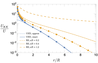
Figure 1: Contribution of the KK-tower in the universal extra dimension model to the Casimir-Polder interaction potential relative to the standard QED (massless photon). The solid (blue) line is the numerical result from Eq. (III.1) obtained truncating the series at $N_{\text{max}}=60$. The full (blue) disks are the results from Eq. (III.1). The dotted (blue) line is the approximated form as given in Eq. (55). The other curves represent the Randall-Sundrum contribution for diffeerent values of the dimensionless parameter $\kappa R$ (with $\xi\to a\xi$ and $a$ given in Eq. 62a) respectivley equal to $0.2$ dashed (orange), $0.4$ dot-dashed (orange) and $1.2$ long-dashed (orange). The full (orange) disks superimposed with the dashed curve represent the result through Eq. III.1 with $\xi\to a\xi$.

IV.2 Randall-Sundrum

In Fig. 1 we also show the contribution of the Randall-Sundrum KK tower relative to the standard Casimir-Polder $U_{KK}/U$ as a function of $\xi=r/R$. As dicussed above the Casimir-Polder interaction in the Randall-Sundrum model is given by the same formulae of the UED case, Eqs. (III.1,III.1,55), with the replacement $\xi\to a\xi$ with $a$ given in Eq. 62a. We show the results for three different values of the dimensionless parameter $\kappa R=0.2,0.4,1.2$. From Fig. 1 we see that the Randall-Sundrum contribution to the Casimir-Polder interaction has a better chance of being non-negligible at values of the distance of experimental interest (nanometers) for larger values of the parameter $\kappa R$. Indeed we find for instance that for a value of $\kappa R=8.2$ and $R\approx 1$ TeV${}^{-1}=3\times 10^{9}\text{nm}^{-1}$ the ratio $U_{KK}/U$ is for $r=10$ nm ($\xi=3.3\times 10^{10}$) about 0.04, or a 4% contribution from the RS model.

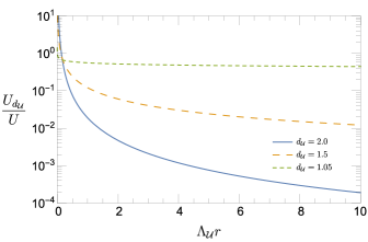
Figure 2: Unparticle Casimir-Polder interaction potential $U_{d_{\cal U}}$ relative to the standard QED (massless photon) Casimir-Polder interaction $U$ as a function of the distance, in units of $\Lambda_{\cal U}^{-1}$, at a fixed value of the coupling $\lambda/e=0.9$. The solid (blue) line is the result for $d_{\cal U}=2$, the long-dashed (orange) line is for $d_{\cal U}=1.5$ result and the short-dashed (green) line is for $d_{\cal U}=1.05$.

IV.3 Unparticles

In Fig. 2 we show the ratio of the Unparticle Casimir-Polder interaction, $U_{d_{\cal U}}$, to the standard massless photon QED Casimir-Polder potential, $U$, versus $\Lambda_{\cal U}r$, or the distance in units of $\Lambda_{\cal U}^{-1}$ for different values of the scaling dimension of the Unparticle field $d_{\cal U}=1.05,1.5,2$.

From Fig. 2 we see that higher values of $d_{\cal U}$ have a better chance of providing a contribution to the Casimir-Polder interaction which has the potential of being measurable. Indeed if we assume a scale of the unparticle model of the order of the TeV, $\Lambda_{\cal U}=1$ TeV ($\approx 3\times 10^{9}$ nm^-1), with $d_{\cal U}=1.05\,\,(\text{and\ }\lambda=0.9)$, we obtain numerically that $U_{d_{\cal U}}/U=0.049$ for typical distances of Casimir experiments in the nano-meter range ($\xi=\Lambda_{\cal U}r\approx 3.3\times 10^{10}$), i.e. a 5% contribution. The fact that the unparticle contribution becomes relevant and possibly detectable only for $d_{\cal U}$ values very close to unity parallels what has been found in the analysis of the Unparticle Casimir effect in ref. Frassino et al. (2017).

V Conclusions

The quite vast current literature of Casimir interactions in relation to a massive photon discusses only the standard Casimir effect in the geometry of two parallel conductor plates. This had been studied in the pioneering work of Barton and Dombey Barton and Dombey (1984, 1985) and subsequently taken up by several authors in other BSM scenarios Frassino and Panella (2012); Blasone et al. (2019); Frank et al. (2007, 2008); Teo (2010b); Poppenhaeger et al. (2004); Frassino et al. (2017); Frassino and Panella (2019); Buoninfante et al. (2019); Lambiase et al. (2017); Blasone et al. (2018); Teo (2010c); Edery and Marachevsky (2008), but always considering the Casimir effect between parallel plates.

In this paper we have studied the intermolecular Casimir-Polder forces between neutral systems at a distance $r$ from each other, mediated by a massive vector field (assuming an electromagnetic-type coupling) thereby filling a gap in the existing literature of Casimir interactions.

Although this might appear at first to be a computation with only a speculative interest it is instead of direct application in deriving the Casimir-Polder interactions between neutral systems in theories beyond the standard model, such as universal extra dimensions (UED), Randall-Sundrum (RS) models and scale invariant theories (Unparticles). Moreover we have discussed the impact of the contributions to the Casimir-Polder interactions in these BSM models relative to the QED contribution and our results could be used to discuss complementary bounds on those BSM theories with future experiments. The above mentioned scenarios are on the other end receiving a lot of attention in other research domains and especially so they are well studied at high energy colliders like the LHC or its future upgrades like the high luminosity or the high energy LHC (HL-LHC or HE-LHC) Cid Vidal et al. (2018), thus highlighting the complementary value of the present work. Specifically we have discussed, within the above BSM scenarios, the deviations of the Casimir-Polder interactions relative to the QED (massless photon) case as a function of the distance $r$ between the neutral systems and in relation to the model free parameters. While the UED contribution to the Casimir-Polder interaction appears to be too small to be measurable in current experiments we have found that both for the RS and the unparticle models there are values of the parameters for which a sizeable contribution would result which could, in principle, be detected.

It is the author’s opinion that even in the absence of observed deviations from the standard QED massless Casimir-Polder one could use the results of the present work to propose bounds on the BSM theories parameter space (at least for the RS and Unparticle cases) that could be compared to those derived from other searches such as the standard Casimir effect and/or even high energy accelerator searches.

References

- Milton (2001) K. A. Milton, The Casimir Effect: Physical Manifestations of Zero-Point Energy (World Scientific, 2001).
- Jaffe (2005) R. L. Jaffe, Phys. Rev. D72, 021301 (2005), arXiv:hep-th/0503158 [hep-th] .
- Graham et al. (2002) N. Graham, R. L. Jaffe, V. Khemani, M. Quandt, M. Scandurra, and H. Weigel, Nucl. Phys. B645, 49 (2002), arXiv:hep-th/0207120 [hep-th] .
- Bordag et al. (2009) M. Bordag, G. L. Klimchitskaya, U. Mohideen, and V. M. Mostepanenko, International Series of Monographs on Physics 145, 1 (2009).
- Casimir and Polder (1948) H. B. G. Casimir and D. Polder, Phys. Rev. 73, 360 (1948).
- Milton (2011) K. A. Milton, American Journal of Physics 79, 697 (2011), https://doi.org/10.1119/1.3573976 .
- Casimir (1949) H. B. G. Casimir, Journal de Chimie Physique 46, 407 (1949).
- Casimir (1948) H. B. G. Casimir, Indag. Math. 10, 261 (1948), [Kon. Ned. Akad. Wetensch. Proc.100N3-4,61(1997)].
- Lamoreaux (1999) S. K. Lamoreaux, Am. J. Phys. 67, 850 (1999).
- Lamoreaux (1997) S. K. Lamoreaux, Phys. Rev. Lett. 78, 5 (1997), [Erratum: Phys. Rev. Lett.81,5475(1998)].
- Mohideen and Roy (1998) U. Mohideen and A. Roy, Phys. Rev. Lett. 81, 4549 (1998).
- Decca et al. (2005) R. Decca, D. López, E. Fischbach, G. Klimchitskaya, D. Krause, and V. Mostepanenko, Annals of Physics 318, 37 (2005), special Issue.
- Decca et al. (2007a) R. S. Decca, D. López, E. Fischbach, G. L. Klimchitskaya, D. E. Krause, and V. M. Mostepanenko, Phys. Rev. D 75, 077101 (2007a).
- Decca et al. (2007b) R. Decca, D. López, E. Fischbach, G. Klimchitskaya, D. Krause, and V. Mostepanenko, The European Physical Journal C 51, 963 (2007b).
- Lamoreaux (2011) S. K. Lamoreaux, in Lecture Notes in Physics, Berlin Springer Verlag, Vol. 834, edited by D. Dalvit, P. Milonni, D. Roberts, and F. da Rosa (2011) p. 219, arXiv:1008.3640 [quant-ph] .
- Bressi et al. (2002) G. Bressi, G. Carugno, R. Onofrio, and G. Ruoso, Phys. Rev. Lett. 88, 041804 (2002).
- Sukenik et al. (1993) C. I. Sukenik, M. G. Boshier, D. Cho, V. Sandoghdar, and E. A. Hinds, Phys. Rev. Lett. 70, 560 (1993).
- Brandt et al. (2008) D. Brandt, G. W. Fraser, D. J. Raine, and C. Binns, J. Low. Temp. Phys. 151, 25 (2008).
- de Medeiros Neto et al. (2012) J. F. de Medeiros Neto, R. O. Ramos, and C. R. Santos, Phys. Rev. D86, 125034 (2012), arXiv:1209.6296 [hep-th] .
- Barton and Dombey (1984) G. Barton and N. Dombey, Nature 311, 336 (1984).
- Barton and Dombey (1985) G. Barton and N. Dombey, Ann. Phys. 162, 231 (1985).
- Belokogne and Folacci (2016) A. Belokogne and A. Folacci, Phys. Rev. D93, 044063 (2016), arXiv:1512.06326 [gr-qc] .
- Tu et al. (2005) L.-C. Tu, J. Luo, and G. T. Gillies, Rept. Prog. Phys. 68, 77 (2005).
- Goldhaber and Nieto (2010) A. S. Goldhaber and M. M. Nieto, Rev. Mod. Phys. 82, 939 (2010), arXiv:0809.1003 [hep-ph] .
- Teo (2011) L. P. Teo, Phys. Lett. B696, 529 (2011), arXiv:1012.2196 [quant-ph] .
- Teo (2010a) L. P. Teo, Phys. Rev. D82, 105002 (2010a), arXiv:1007.4397 [quant-ph] .
- Teo (2012) L. P. Teo, J. Math. Phys. 53, 102302 (2012), arXiv:1206.4378 [quant-ph] .
- Frassino and Panella (2012) A. M. Frassino and O. Panella, Phys.Rev. D85, 045030 (2012).
- Blasone et al. (2019) M. Blasone, G. Lambiase, G. G. Luciano, L. Petruzziello, and F. Scardigli, (2019), arXiv:1902.02414 [hep-th] .
- Frank et al. (2007) M. Frank, I. Turan, and L. Ziegler, Phys. Rev. D 76, 015008 (2007).
- Frank et al. (2008) M. Frank, N. Saad, and I. Turan, Phys. Rev. D 78, 055014 (2008).
- Teo (2010b) L. P. Teo, Phys. Rev. D82, 027902 (2010b), arXiv:1007.1810 [hep-th] .
- Poppenhaeger et al. (2004) K. Poppenhaeger, S. Hossenfelder, S. Hofmann, and M. Bleicher, Phys. Lett. B 582, 1 (2004).
- Frassino et al. (2017) A. M. Frassino, P. Nicolini, and O. Panella, Phys. Lett. B772, 675 (2017), arXiv:1311.7173 [hep-ph] .
- Frassino and Panella (2019) A. M. Frassino and O. Panella, (2019), arXiv:1907.00733 [hep-th] .
- Caffarelli and Silvestre (2007) L. Caffarelli and L. Silvestre, Communications in Partial Differential Equations 32, 1245 (2007).
- Buoninfante et al. (2019) L. Buoninfante, G. Lambiase, L. Petruzziello, and A. Stabile, Eur. Phys. J. C79, 41 (2019), arXiv:1811.12261 [gr-qc] .
- Lambiase et al. (2017) G. Lambiase, A. Stabile, and A. Stabile, Phys. Rev. D95, 084019 (2017), arXiv:1611.06494 [gr-qc] .
- Blasone et al. (2018) M. Blasone, G. Lambiase, L. Petruzziello, and A. Stabile, Eur. Phys. J. C78, 976 (2018), arXiv:1808.04425 [hep-th] .
- Teo (2010c) L. P. Teo, JHEP 10, 019 (2010c), arXiv:1008.2044 [hep-th] .
- Edery and Marachevsky (2008) A. Edery and V. Marachevsky, J. High Energy Phys. 0812, 035 (2008), arXiv:0810.3430 [hep-th] .
- Panella (2007) O. Panella, Phys.Rev. D76, 045012 (2007).
- Riahi (1972) F. Riahi, American Journal of Physics 40, 386 (1972), https://doi.org/10.1119/1.1986557 .
- Greiner et al. (2013) W. Greiner, D. Bromley, and J. Reinhardt, Field Quantization (Springer Berlin Heidelberg, 2013).
- Berestetskii et al. (2012) V. Berestetskii, L. Pitaevskii, and E. Lifshitz, Quantum Electrodynamics (Elsevier Science, 2012).
- Note (1) Or by replacing the polarizabilities with the mean polarizabilities .
- Fabiano and Panella (2010) N. Fabiano and O. Panella, Phys. Rev. D81, 115001 (2010), arXiv:0804.3917 [hep-ph] .
- Appelquist et al. (2001) T. Appelquist, H.-C. Cheng, and B. A. Dobrescu, Phys. Rev. D 64, 035002 (2001).
- Macesanu et al. (2002) C. Macesanu, C. McMullen, and S. Nandi, Physics Letters B 546, 253 (2002).
- Rizzo (2001) T. G. Rizzo, Phys. Rev. D 64, 095010 (2001).
- Aad et al. (2015) G. Aad et al. (ATLAS Collaboration), JHEP 04, 116 (2015), arXiv:1501.03555 [hep-ex] .
- Beuria et al. (2018) J. Beuria, A. Datta, D. Debnath, and K. T. Matchev, Comput. Phys. Commun. 226, 187 (2018), arXiv:1702.00413 [hep-ph] .
- Bélanger et al. (2011) G. Bélanger, M. Kakizaki, and A. Pukhov, Journal of Cosmology and Astroparticle Physics 2011, 009 (2011).
- Pascoal et al. (2008) F. Pascoal, L. F. A. Oliveira, F. S. S. Rosa, and C. Farina, Brazilian Journal of Physics 38, 581 (2008), hep-th/0701181 .
- Abramowitz and Stegun (1964) M. Abramowitz and I. A. Stegun, Handbook of Mathematical Functions with Formulas, Graphs, and Mathematical Tables, ninth dover printing, tenth gpo printing ed. (Dover, New York, 1964).
- Randall and Sundrum (1999a) L. Randall and R. Sundrum, Phys. Rev. Lett. 83, 3370 (1999a).
- Randall and Sundrum (1999b) L. Randall and R. Sundrum, Phys. Rev. Lett. 83, 4690 (1999b).
- Teo (2010d) L. P. Teo, Journal of High Energy Physics 2010, 19 (2010d).
- Georgi (2007) H. Georgi, Phys. Rev. Lett. 98, 221601 (2007).
- Banks and Zaks (1982) T. Banks and A. Zaks, Nucl.Phys. B196, 189 (1982).
- Grinstein et al. (2008) B. Grinstein, K. Intriligator, and I. Z. Rothstein, Phys. Lett. B 662, 367 (2008).
- Farina (2006) C. Farina, 26th Brazilian National Meeting on Particles and Fields (ENFPC 2005) Sao Lourenco, Brazil, October 4-8, 2005, Braz. J. Phys. 36, 1137 (2006), arXiv:hep-th/0612232 [hep-th] .
- Milton et al. (1978) K. A. Milton, L. L. DeRaad, Jr., and J. S. Schwinger, Annals Phys. 115, 388 (1978).
- Milton and Ng (1998) K. A. Milton and Y. J. Ng, Phys. Rev. E57, 5504 (1998), arXiv:hep-th/9707122 [hep-th] .
- Olver et al. (2010) F. W. Olver, D. W. Lozier, R. F. Boisvert, and C. W. Clark, NIST Handbook of Mathematical Functions, 1st ed. (Cambridge University Press, New York, NY, USA, 2010).
- Choudhury and Ghosh (2016) D. Choudhury and K. Ghosh, Phys. Lett. B763, 155 (2016), arXiv:1606.04084 [hep-ph] .
- Klimchitskaya et al. (2009) G. L. Klimchitskaya, U. Mohideen, and V. M. Mostepanenko, Rev. Mod. Phys. 81, 1827 (2009).
- Cid Vidal et al. (2018) X. Cid Vidal et al. (Working Group 3, Cern Yellow Report), (2018), arXiv:1812.07831 [hep-ph] .