Eliashberg equations for an electron-phonon version of the Sachdev-Ye-Kitaev model: Pair Breaking in non-Fermi liquid superconductors

Abstract

We present a theory that is a non-Fermi-liquid counterpart of the Abrikosov-Gor’kov pair-breaking theory due to paramagnetic impurities in superconductors. To this end we analyze a model of interacting electrons and phonons that is a natural generalization of the Sachdev-Ye-Kitaev-model. In the limit of large numbers of degrees of freedom, the Eliashberg equations of superconductivity become exact and emerge as saddle-point equations of a field theory with fluctuating pairing fields. In its normal state the model is governed by two non-Fermi liquid fixed points, characterized by distinct universal exponents. At low temperatures a superconducting state emerges from the critical normal state. We study the role of pair-breaking on $T_{c}$, where we allow for disorder that breaks time-reversal symmetry. For small Bogoliubov quasi-particle weight, relevant for systems with strongly incoherent normal state, $T_{c}$ drops rapidly as function of the pair breaking strength and reaches a small but finite value before it vanishes at a critical pair-breaking strength via an essential singularity. The latter signals a breakdown of the emergent conformal symmetry of the non-Fermi liquid normal state.

1 Introduction

The dynamical theory of phonon-mediated superconductivity was formulated by Gerasim Matveevich Eliashberg in a pioneering tour de force of quantum many-body theory[1, 2]. Considering the regime where phonon frequencies are much smaller than the Fermi energy of the electrons, electrons follow the lattice motion almost instantly. In this limit, Migdal had shown that electron-phonon vertex corrections become small[3]. Then a complicated intermediate-coupling problem suddenly becomes tractable. A closed, self-consistent dynamical theory emerges that is not limited to the regime of weak electron-phonon interactions. The Eliashberg formalism follows the Gor’kov-Nambu description of superconductivity[4, 5], reflecting the broken global $U\left(1\right)$ symmetry, associated with charge conservation. The propagation of particles and the conversion of particles into holes are described by two self energies $\Sigma\left(\omega\right)$ and $\Phi\left(\omega\right)$, respectively. Using the Eliashberg theory, important advances were made in understanding the physical properties of superconductors with a dimensionless electron-phonon coupling of order unity[6, 7, 8, 9, 10, 11, 12].

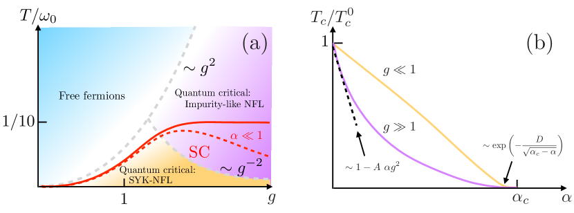
Figure 1: (a) Schematic phase diagram obtained from solving the Eliashberg equations, Eq.(9). Normal state properties are independent of pair breaking parameter $\alpha$. The solid red line is superconducting $T_{c}$ for $\alpha=0$; dashed red line is $T_{c}$ for a small non-zero value of $\alpha\ll 1$. For $\alpha$ small, $T_{c}$ is weakly affected at weak coupling $g\ll 1$. However, for strong coupling $g\gg 1$ even small $\alpha$ dramatically depresses $T_{c}$. (b) Schematic plot of superconducting $T_{c}$ as a function of pair breaking parameter $\alpha$, normalized by $T_{c}^{0}=T_{c}(\alpha=0)$. In the weak coupling regime $T_{c}(\alpha)/T_{c}^{0}$ follows a $g$-independent universal curve. In the strong coupling regime $T_{c}$ drops linearly with $\alpha g^{2}$ for small $\alpha$, so that $T_{c}$ is already significantly reduced for $\alpha\sim 1/g^{2}$. $T_{c}(\alpha)$ extends to a $g$-independent critical value $\alpha_{c}$. Near $\alpha_{c}$ the transition temperature obeys a BKT-scaling $T_{c}\sim\exp(-D/\sqrt{\alpha_{c}-\alpha})$.

The Eliashberg formalism has been applied to study superconductivity in problems that go significantly beyond the original electron-phonon problem[13, 14, 15, 16, 17, 18, 19, 20, 21, 22, 23]. When an electronic system becomes quantum critical, soft degrees of freedom emerge. The retarded nature of the coupling to such soft excitations makes an analysis in the spirit Eliashberg’s approach, with a dynamical pairing field $\Phi\left(\omega\right)$, natural. Since realistic models of quantum critical pairing usually possess no natural small parameter, a controlled approach that leads to an Eliashberg-like formalism is highly desirable.

Recently, two of us introduced and solved a model for the electron-phonon interaction in non-Fermi liquids[24]. It is a natural generalization of the Sachdev-Ye-Kitaev (SYK) model[25, 26, 27, 28, 29] and yields superconductivity due to electron-phonon interactions with quantum critical behavior in the normal state. The model becomes solvable in the limit of infinite number of degrees of freedom. The Eliashberg equations of superconductivity, with self-consistently determined electron and phonon propagators, become exact. The formalism yields rich non-Fermi liquid behavior in the normal state and gives rise to superconductivity at low temperatures. Related interesting descriptions of superconductivity in SYK-like models have also been discussed in Refs.[30, 31, 32]. While SYK models are dominated by random interactions, the belief is that the non-Fermi liquid behavior that occurs is in fact more general and may also offer insights into non-random systems.

In its normal state the model of Ref.[24] is governed by two non-Fermi liquid fixed points, characterized by distinct universal exponents. The weakened ability of such non-Fermi liquid electronic states to form Cooper pairs is offset by an increasingly singular pairing interaction, leading to coherent superconductivity in such incoherent systems. This result is closely related to the generalized Cooper theorem of quantum-critical pairing put forward by Abanov et al. in Ref.[15]. In Ref.[24] the ground state was shown to be characterized by sharp Bogoliubov quasiparticles. However, the incoherent nature of the normal-state leads to a much reduced spectral weight $Z_{B}$ of the Bogoliubov quasiparticles. For small values of $Z_{B}$ a reduction in the condensation energy occurs. At the same time, the transition temperature remains unchanged. This behavior is reminiscent of superconductivity in systems with non-pair-breaking impurities, where Anderson’s theorem guarantees an unchanged transition temperature, while the superconducting state becomes more fragile the larger the disorder strength, with e.g. a strongly reduced superfluid stiffness[33, 34, 35].

An important issue in the investigation of superconducting states is their robustness with respect to pair-breaking disorder. The topic was pioneered by Abrikosov and Gor’kov, who analyzed the role of paramagnetic impurities in conventional superconductors[36] and found a suppression of $T_{c}$ determined by $\log\left(T_{c}^{0}/T_{c}\right)=\psi\left(\frac{1}{2}-\frac{1}{2\pi\tau T_{c}}\right)-\psi\left(\frac{1}{2}\right)$ with scattering rate due to paramagnetic impurities $\tau^{-1}$ and digamma function $\psi$. $T_{c}^{0}$ is the transition temperature without pair breaking. The inclusion of quantum dynamics of the impurities, unconventional pairing states, critical normal states, and strong impurity scattering are topics of ongoing theoretical investigations, see e.g. Refs.[37, 38, 39, 40, 41, 42, 43, 44, 45, 46, 47, 48, 49, 50, 51, 52, 54, 53, 55, 56, 57] for an incomplete list of publications. In this context an interesting question is the nature by which superconductivity vanishes due to pair breaking if the normal state is quantum critical.

In this paper we generalize the electron-phonon SYK model to analyze the robustness of pairing in quantum-critical systems against pair-breaking effects due to time-reversal symmetry violation. We solve the modified Eliashberg equations and find a suppression of the transition temperature as a function of a pair-breaking parameter $\alpha$, with $T_{c}$ vanishing at a critical pair-breaking strength $\alpha_{c}$. While the qualitative trends are similar to the Abrikosov-Gor’kov theory[36], there are key distinctions in the overall dependence of $T_{c}$ on $\alpha$. Near $\alpha_{c}\approx 0.62$, we find a behavior

$$T_{c}\left(\alpha\approx\alpha_{c}\right)=T^{*}\exp\left(-\frac{D}{\sqrt{\alpha_{c}-\alpha}}\right),$$ (1)

where $D$ is a non-universal constant and $T^{*}$ an energy scale that we discuss below. This behavior is similar to the scaling near a Berezinskii-Kosterlitz-Thouless (BKT) transition[58, 59]. Such BKT-scaling was argued to be generic for systems with a transition from a conformal to a non-conformal phase[60]. Given the conformal symmetry of the SYK model[26], which is relevant to our normal state, the result Eq.(1) for the superconducting transition temperature is further confirmation of the expectation put forward in Ref.[60]. Thus, the change of the superconducting transition temperature as function of a pair-breaking impurity concentration may serve as a tool to identify whether a normal state can be effectively thought of as a critical state with an underlying conformal symmetry. A behavior like that of Eq.(1) occurs in the coupling constant dependence of the mass scale near the chiral symmetry breaking point of $2+1$-dimensional quantum electrodynamics[61]. In the context of coherent versus incoherent pairing, such behavior was first seen in an Eliashberg theory near a magnetic instability in Ref.[15]. An interesting renormalization group perspective of Eq.(1) in the context of superconductivity was recently given in Ref.[20]. An appeal of our approach is that the critical coupling $\alpha_{c}$ in Eq.(1) acquires a clear physical and potentially tunable interpretation as a pair-breaking parameter due to time-reversal symmetry breaking disorder.

In addition to the behavior near the critical pair-breaking strength $\alpha_{c}$ we also analyze the interplay between normal-state incoherency and the robustness of superconductivity with respect to pair breaking. In the incoherent, strong coupling regime of the system, we find that $T_{c}$ is already substantially suppressed for $\alpha\approx\alpha^{*}\ll\alpha_{c}$, where the crossover scale $\alpha^{*}\sim Z_{B}$ is proportional to the small Bogoliubov quasiparticle weight for $\alpha=0$, i.e.

$$T_{c}\left(\alpha\sim Z_{B}\right)\ll T_{c}^{0},$$ (2)

with $T_{c}^{0}=T_{c}\left(\alpha=0\right)$. Thus, a pairing state that emerges from an incoherent normal state with small $Z_{B}$ is particularly fragile against pair breaking. These findings are summarized in Fig.1b.

In what follows we introduce our model, show that the solution is given by a set of coupled Eliashberg equations, and present the solution of this set of equations.

2 Eliashberg equations

We start from the Hamiltonian

$$H = -\mu\sum_{i=1}^{N}\sum_{\sigma=\pm}c_{i\sigma}^{\dagger}c_{i\sigma}+\frac{1}{2}\sum_{k=1}^{M}\left(\pi_{k}^{2}+\omega_{0}^{2}\phi_{k}^{2}\right)+\frac{1}{N}\sum_{ij,\sigma}^{N}\sum_{k}^{M}g_{ij,k}c_{i\sigma}^{\dagger}c_{j\sigma}\phi_{k},$$ (3)

with electron annihilation and creation operators $c_{i\sigma}$ and $c_{i\sigma}^{\dagger}$, respectively, that obey $\left[c_{i\sigma},c_{j\sigma^{\prime}}^{\dagger}\right]_{+}=\delta_{ij}$$\delta_{\sigma\sigma^{\prime}}$ and $\left[c_{i\sigma},c_{j\sigma}\right]_{+}=0$ with spin $\sigma=\pm 1$. In addition we have phonons $\phi_{k}$ with canonical momentum $\pi_{k}$, such that $\left[\phi_{k},\pi_{k^{\prime}}\right]_{-}=i\delta_{kk^{\prime}}$. Here $i,j=1\cdots N$ refer to electrons and $k=1\cdots M$ to the phonons. In what follows we mostly consider the limit $N=M$.

The problem becomes solvable because of the fully-connected nature of the electron-phonon interaction. The electron-phonon coupling constants $g_{ij,k}$ are Gaussian-distributed random variables that obey $g_{ij,k}=g_{ji,k}^{*}.$ The coupling constants are in general complex valued $g_{ij,k}=g_{ij,k}^{{}^{\prime}}+ig_{ij,k}^{{}^{\prime\prime}}$ with real part $g_{ij,k}^{{}^{\prime}}$ and imaginary part $g_{ij,k}^{{}^{\prime\prime}}$. In what follows we will use a distribution function with zero mean and second moment given by

$$\overline{g_{ij,k}^{{}^{\prime}}g_{i^{\prime}j^{\prime},k^{\prime}}^{{}^{\prime}}} = \left(1-\frac{\alpha}{2}\right)\bar{g}^{2}\delta_{k,k^{\prime}}\left(\delta_{ii^{\prime}}\delta_{jj^{\prime}}+\delta_{ij^{\prime}}\delta_{ji^{\prime}}\right),$$

$$\overline{g_{ij,k}^{{}^{\prime\prime}}g_{i^{\prime}j^{\prime},k^{\prime}}^{{}^{\prime\prime}}} = \frac{\alpha}{2}\bar{g}^{2}\delta_{k,k^{\prime}}\left(\delta_{ii^{\prime}}\delta_{jj^{\prime}}-\delta_{ij^{\prime}}\delta_{ji^{\prime}}\right),$$

$$\overline{g_{ij,k}^{{}^{\prime}}g_{i^{\prime}j^{\prime},k^{\prime}}^{{}^{\prime\prime}}} = 0.$$ (4)

The over-bar denotes disorder averages. The two limits $\alpha=0$ and $\alpha=1$ were discussed previously in Ref.[24]. In the former case, the coupling constants are all real valued with $g_{ij,k}=g_{ji,k}$. For given $k$, the $g_{ij,k}$ are then chosen from the Gaussian orthogonal ensemble of random matrices[62]. Time-reversal symmetry of the Hamiltonian is not only preserved on average, but also for each individual realization of the $g_{ij,k}$. As a result, the electron-phonon interaction of Eq.(3) induces superconductivity. On the other hand, for $\alpha=1$, each configuration of the coupling constants, distributed according to the Gaussian unitary ensemble, strongly breaks time-reversal symmetry and no superconductivity occurs. Instead, a non-Fermi liquid normal state emerges where the spectral functions of electrons and phonons are governed by universal power laws, a behavior that is qualitatively similar to the usual formulation of the SYK model with random four-fermion interactions[25, 26, 27, 28, 29]. Below we will summarize the main finding of these limits in greater detail.

For $0<\alpha<1$ the breaking of time-reversal symmetry is intermediate. In particular, for small $\alpha$ one expects that superconductivity should survive albeit with a reduced transition temperature. Thus, $\alpha$ plays the role of a dimensionless pair-breaking parameter that characterizes the relative importance of time-reversal symmetry breaking disorder.

To proceed, we use the replica trick[63] to perform the disorder average

$$\overline{e^{-S_{{\rm rdm}}}}=\overline{e^{-\sum_{ijk}g_{ijk}O_{ijk}}},$$ (5)

where $O_{ijk}=\frac{1}{N}\sum_{\sigma a}\int_{0}^{\beta}d\tau c_{i\sigma a}^{\dagger}\left(\tau\right)c_{j\sigma a}\left(\tau\right)\phi_{ka}\left(\tau\right).$ Here, $a=1,\cdots,n$ is the replica index while $\tau$ stands for the imaginary time in the Matsubara formalism with $\beta=\left(k_{B}T\right)^{-1}$ the inverse temperature. Using the Gaussian disorder distribution, characterized by Eq.(4), we obtain for the disorder average

$$\overline{e^{-\sum_{ijk}g_{ijk}O_{ijk}}}=e^{\frac{1}{4}\left(1-\frac{\alpha}{2}\right)\bar{g}^{2}\sum_{ijk}\left(O_{ijk}^{\dagger}+O_{ijk}\right)^{2}-\frac{\alpha}{8}\bar{g}^{2}\sum_{ijk}\left(O_{ijk}^{\dagger}-O_{ijk}\right)^{2}}.$$ (6)

For the Gaussian unitary ensemble with $\alpha=1$ only terms like $O_{ijk}^{\dagger}O_{ijk}$, occur. On the other hand, for $\alpha<1$ we find in addition anomalous terms $O_{ijk}^{\dagger}O_{ijk}^{\dagger}$ and $O_{ijk}O_{ijk}$. These terms give rise to anomalous self energies and propagators and, if the self energies aquire a finite mean value, to superconductivity.

To proceed, we introduce collective variables through the identities

$$1 = \int{\cal D}G{\cal D}\Sigma e^{\sum_{ab,\sigma\sigma^{\prime}}\int d\tau d\tau^{\prime}\left(NG_{ba,\sigma^{\prime}\sigma}\left(\tau^{\prime},\tau\right)-\sum_{i}c_{i\sigma a}^{\dagger}\left(\tau\right)c_{i\sigma^{\prime}b}\left(\tau^{\prime}\right)\right)\Sigma_{ab,\sigma\sigma^{\prime}}\left(\tau,\tau^{\prime}\right)},$$

$$1 = \int{\cal D}F{\cal D}\Phi e^{\sum_{ab,\sigma\sigma^{\prime}}\int d\tau d\tau^{\prime}\left(NF_{ba,\sigma^{\prime}\sigma}\left(\tau^{\prime},\tau\right)-\sum_{i}c_{i\sigma a}\left(\tau\right)c_{i\sigma^{\prime}b}\left(\tau^{\prime}\right)\right)\Phi_{ab,\sigma\sigma^{\prime}}^{+}\left(\tau,\tau^{\prime}\right)},$$

$$1 = \int{\cal D}F^{*}{\cal D}\Phi^{{}^{*}}e^{\sum_{ab,\sigma\sigma^{\prime}}\int d\tau d\tau^{\prime}\left(NF_{ba,\sigma^{\prime}\sigma}\left(\tau^{\prime},\tau\right)-\sum_{i}c_{i\sigma a}^{\dagger}\left(\tau\right)c_{i\sigma^{\prime}b}^{\dagger}\left(\tau^{\prime}\right)\right)\Phi_{ab,\sigma\sigma^{\prime}}^{+}\left(\tau,\tau^{\prime}\right)},$$

$$1 = \int{\cal D}D{\cal D}\Pi e^{\frac{1}{2}\sum_{ab}\int d\tau d\tau^{\prime}\left(ND_{ba}\left(\tau^{\prime},\tau\right)-\sum_{i}\phi_{ia}\left(\tau\right)\phi_{ib}\left(\tau^{\prime}\right)\right)\Pi_{ab}\left(\tau,\tau^{\prime}\right)}.$$

This allows one to integrate out the electron and phonon degrees of freedom, which yields for replica symmetric solutions and singlet pairing the effective action

$$S = -N{\rm tr}\log\left(\hat{G}_{0}^{-1}-\hat{\Sigma}\right)+\frac{N}{2}{\rm tr}\log\left(D_{0}^{-1}-\Pi\right)$$ (7)

$$- 2N\int d\tau d\tau^{\prime}G\left(\tau^{\prime},\tau\right)\Sigma\left(\tau,\tau^{\prime}\right)+\frac{N}{2}\int d\tau d\tau^{\prime}D\left(\tau^{\prime},\tau\right)\Pi\left(\tau,\tau^{\prime}\right)$$

$$- N\int d\tau d\tau^{\prime}\left(F\left(\tau^{\prime},\tau\right)\Phi\left(\tau,\tau^{\prime}\right)+F^{*}\left(\tau^{\prime},\tau\right)\Phi^{*}\left(\tau,\tau^{\prime}\right)\right)$$

$$+ N\overline{g}^{2}\int d\tau d\tau^{\prime}\left(\left|G\left(\tau,\tau^{\prime}\right)\right|^{2}-\left(1-\alpha\right)F^{*}\left(\tau,\tau^{\prime}\right)F\left(\tau^{\prime},\tau\right)\right)D\left(\tau,\tau^{\prime}\right).$$

Here,

$$\hat{\Sigma}\left(\tau,\tau^{\prime}\right)=\left(\begin{array}[]{cc}\Sigma\left(\tau,\tau^{\prime}\right)&\Phi\left(\tau,\tau^{\prime}\right)\\ \Phi^{*}\left(\tau,\tau^{\prime}\right)&-\Sigma\left(\tau^{\prime},\tau\right)\end{array}\right)$$ (8)

is a matrix in Nambu space. In the limit $N\rightarrow\infty$ the integration over the collective variables can be performed through the saddle-point method and we obtain time-translation invariant solutions. After Fourier transformation to Matsubara frequencies the saddle-point equations take the form of the Eliashberg equations:

$$i\epsilon_{n}\left(1-Z\left(\epsilon_{n}\right)\right) = -\bar{g}^{2}T\sum_{n^{\prime}}\frac{D\left(\epsilon_{n}-\epsilon_{n^{\prime}}\right)i\epsilon_{n^{\prime}}Z\left(\epsilon_{n^{\prime}}\right)}{\left(\epsilon_{n^{\prime}}Z\left(\epsilon_{n^{\prime}}\right)\right)^{2}+\Phi\left(\epsilon_{n^{\prime}}\right)^{2}},$$

$$\Phi\left(\epsilon_{n}\right) = \left(1-\alpha\right)\bar{g}^{2}T\sum_{n^{\prime}}\frac{D\left(\epsilon_{n}-\epsilon_{n^{\prime}}\right)\Phi\left(\epsilon_{n^{\prime}}\right)}{\left(\epsilon_{n^{\prime}}Z\left(\epsilon_{n^{\prime}}\right)\right)^{2}+\Phi\left(\epsilon_{n^{\prime}}\right)^{2}},$$

$$\Pi\left(\nu_{n}\right) = -2\bar{g}^{2}T\sum_{n^{\prime}}\left(G\left(\epsilon_{n^{\prime}}+\nu_{n}\right)G\left(\epsilon_{n}\right)-\left(1-\alpha\right)F\left(\epsilon_{n^{\prime}}+\nu_{n}\right)F\left(\epsilon_{n^{\prime}}\right)\right),$$ (9)

where $\Sigma\left(\epsilon_{n}\right)=i\epsilon_{n}\left(1-Z\left(\epsilon_{n}\right)\right)$.

$$D\left(\nu_{n}\right)=\frac{1}{\nu_{n}^{2}+\omega_{0}^{2}-\Pi\left(\nu_{n}\right)}$$ (10)

is the phonon propagator, while the electron propagator in Nambu space is $\hat{G}^{-1}\left(\epsilon_{n}\right)=\hat{G}_{0}^{-1}-\hat{\Sigma}\left(\epsilon_{n}\right)$ with $\hat{G}_{0}^{-1}(\epsilon_{n})=i\epsilon_{n}\hat{1}$. Here $\epsilon_{n}$=$\left(2n+1\right)\pi T$ and $\nu_{n}=2n\pi T$ are fermionic and bosonic Matsubara frequencies, respectively.

One immediately observes that in the normal state, with $\Phi=F=0$, the solution of this set of equations is independent of the pair-breaking parameter $\alpha$. Before we analyze the dependence of superconductivity on $\alpha$ we briefly summarize the regimes $\alpha=1$ and $\alpha=0$ that were discussed already in Ref.[24].

For $\alpha=1$, time reversal symmetry is strongly broken and no superconducting solution exists. In the phase diagram as a function of temperature and dimensionless coupling constant $g=\bar{g}/\omega_{0}^{3/2}$, shown in Fig.1a, we find three distinct regimes: i) for $T\gg T_{f}\sim g^{2}\omega_{0}$ interactions are irrelevant and the systems behaves as free fermions and bosons. ii) for $T<T^{*}$ with $T^{*}\sim\omega_{0}\min\left(g^{2},g^{-2}\right)$ we find a fermionic self energy $\Sigma\left(\epsilon_{n}\right)=-c_{1}i\epsilon_{n}\left|g^{2}\omega_{0}/\epsilon_{n}\right|^{2\Delta}$. For the dynamic part of the bosonic self energy, $\delta\Pi\left(\nu_{n}\right)\equiv\Pi\left(\nu_{n}\right)-\Pi\left(0\right)$, we obtain $\delta\Pi\left(\nu_{n}\right)=c_{3}\left|\nu_{n}/\left(g^{2}\omega_{0}\right)\right|^{4\Delta-1}\omega_{0}^{2}$. The renormalized phonon frequency $\omega_{r}^{2}=\omega_{0}^{2}-\Pi\left(0\right)$ behaves as $\omega_{r}^{2}=c_{2}\left(T/\left(g^{2}\omega_{0}\right)\right)^{4\Delta-1}\omega_{0}^{2}$. The numerical coefficients $c_{1}\approx 1.155$, $c_{2}\approx 0.561$, and $c_{3}\approx 0.710$ were determined in Ref.[24]. The scaling dimension of the fermions was found to be $\Delta\approx 0.4203$. This exponent determines the phonon dynamics via the anomalous Landau damping term $\delta\Pi\left(\nu_{n}\right)$. Notice, for $g<1$ it holds that $T_{f}\sim T^{*}$. In this regime an emergent conformal symmetry characterizes the low energy and low temperature behavior. iii) For $g>1$ there exists an intermediate temperature regime $g^{-2}<T/\omega_{0}<g^{2}$, i.e. $T^{*}<T<T_{f}$, where the phonons are long-lived and have a renormalized frequency $\omega_{r}^{2}=\left(\frac{3\pi}{8}\right)^{2}T\omega_{0}/g^{2}$. At the same time the fermionic self energy is impurity-like, $\Sigma\left(\epsilon_{n}\right)=-i{\rm sign}\left(\epsilon_{n}\right)\frac{8}{3\pi}g^{2}\omega_{0}$, a behavior caused by the coupling of electrons to very soft, i.e. almost classical, phonons.

For $\alpha=0$, superconductivity emerges at a critical temperature $T_{c}^{0}\left(g\ll 1\right)\approx 0.16g^{2}\omega_{0}$, while for large $g$ the transition temperature saturates, $T_{c}^{0}\left(g\gg 1\right)\approx 0.112\omega_{0}$. In the strong coupling regime, the weight of the Bogoliubov quasiparticles behaves as $Z_{B}\sim g^{-2}$ while the ratio $\frac{2\Delta_{0}}{T_{c}}\approx 11.46$ with superconducting gap $\Delta_{0}$ and the transition temperature $T_{c}$ is significantly larger then the BCS value. We summarize the key regimes of the normal state and the transition temperature in Fig.1a. The fact that $T_{c}(g\ll 1,\alpha=0)$ saturates is a consequence of the Anderson theorem where impurities and soft bosons that do not break time reversal symmetry will not cause a suppression of the transition temperature.

3 Pair Breaking

3.1 Numerical analysis and gap equations in the scaling limit

We first present the results obtained from a complete numerical solution of the coupled Eliashberg equations. In Fig.2 we show the superconducting transition temperature as a function of the pair-breaking parameter $\alpha$ for varying dimensionless coupling strength $g$. While $T_{c}\left(\alpha\right)$ is weakly $g$-dependent for small $g$, we find a strong variation of the initial suppression of the transition temperature in the strong coupling limit $g>1$. $T_{c}\left(\alpha\right)$ seems to vanish at a $g$-independent critical value $\alpha_{c}$. While the numerical convergence at large $g$ is poor at lowest temperatures, a behavior consistent with Eq.(1) can clearly be seen for smaller $g$; see in particular the inset of Fig.3.

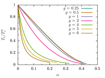
Figure 2: Superconducting transition temperature $T_{c}\left(\alpha\right)$ as function of the dimensionless pair breaking parameter for different dimensionless coupling strength $g$. For small $g$, $T_{c}\left(\alpha\right)$ follows a weakly $g$-dependent universal curve, while the initial drop with the pair breaking strength depends sensitively on the coupling constant for larger $g$. All curves seem to extend to a $g$-independent critical value $\alpha_{c}$. The full numerical solution converges poorly at low $T$ and large $g$, a regime that will be analyzed by solving the linearized gap equation using analytically determined scaling solutions for the normal-state electron and phonon propagators.

In order to obtain a more detailed understanding of these results we analyze the linearized gap equations in the scaling limit. If we linearize with respect to the anomalous self energy and combine the Eliashberg equations for $Z\left(\epsilon_{n}\right)$ and $\Phi\left(\epsilon_{n}\right)$ to determine the gap function $\Delta\left(\epsilon_{n}\right)=\Phi\left(\epsilon_{n}\right)/Z\left(\epsilon_{n}\right)$, we obtain

$$\Delta\left(\epsilon_{n}\right)=\bar{g}^{2}T_{c}\sum_{n^{\prime}}\frac{D\left(\epsilon_{n}-\epsilon_{n^{\prime}}\right)}{Z\left(\epsilon_{n^{\prime}}\right)\epsilon_{n^{\prime}}}\left(\left(1-\alpha\right)\frac{\Delta\left(\epsilon_{n^{\prime}}\right)}{\epsilon_{n^{\prime}}}-\frac{\Delta\left(\epsilon_{n}\right)}{\epsilon_{n}}\right).$$ (11)

Here $D\left(\nu_{n}\right)=\left(\nu_{n}^{2}+\omega_{r}^{2}-\delta\Pi\left(\nu_{n}\right)\right)$ and $Z\left(\epsilon_{n}\right)=1-i\Sigma\left(\epsilon_{n}\right)/\epsilon_{n}$ are the self-consistently determined normal state boson propagator and fermion self energy. For $\alpha=0$ the zeroth bosonic Matsubara frequency, i.e. $n=n^{\prime}$, does not contribute to the gap equation. This ensures that only quantum fluctuations of phonons influence the value of $T_{c}$. Even very soft bosons do not act as pair-breakers, in accordance with Anderson’s theorem [33, 34, 35]. The situation changes for finite $\alpha$. Now the zeroth Matsubara frequency contributes to the gap equation and soft bosons become pair breaking.

For $T<T^{*}$, the normal state boson propagator and fermion self energy are governed by the SYK-like scaling regime. Inserting these results, we obtain the following expression for the linearized gap equation:

$$\Delta\left(\epsilon_{n}\right)=\frac{1}{2\pi C_{\Delta}}\sum_{n^{\prime}}\frac{\left(\frac{T_{f}}{T_{c}}\right)^{2\Delta}}{m_{0}+\left|n-n^{\prime}\right|^{4\Delta-1}}\frac{\left(1-\alpha\right)\frac{\Delta\left(\epsilon_{n^{\prime}}\right)}{n^{\prime}+\frac{1}{2}}-\frac{\Delta\left(\epsilon_{n}\right)}{n+\frac{1}{2}}}{\left(n^{\prime}+\frac{1}{2}\right)\left(\left(\frac{T_{c}}{T_{f}}\right)^{2\Delta}+\left|n^{\prime}+\frac{1}{2}\right|^{-2\Delta}\right)}.$$ (12)

where $m_{0}=\frac{c_{2}}{c_{3}\left(2\pi\right)^{4\Delta-1}}\approx 0.157$ and $C_{\Delta}=-8\cos\left(\pi\Delta\right)\sin^{3}\left(\pi\Delta\right)\Gamma\left(2\Delta\right)^{2}\Gamma\left(1-4\Delta\right)/\pi^{2}$ such that $\frac{1}{2\pi C_{\Delta}}\approx 0.168212$. Here $T_{f}=\frac{1}{2\pi}c_{1}^{\frac{1}{2\Delta}}g^{2}\omega_{0}\approx 0.189g^{2}\omega_{0}$. Because the temperature only appears in the combination $T/T_{f}$, in this regime we must have $T_{c}=T_{f}F(\alpha)$ for some function $F$. Furthermore, in the weak-coupling regime $g\ll 1$ we have $T_{f}\sim T_{c}^{0}\sim g^{2}$, so that $T_{c}/T_{c}^{0}$ is independent of $g$. This explains the $g$-independence of $T_{c}(\alpha)$ in the weak-coupling regime, observed in Fig.2. Gap equations similar to the one of Eq.(12) were recently discussed in Ref.[21, 22, 23], pointing out that superconductivity remains robust despite the incoherent nature of the normal state because the self-energy from dynamic critical fluctuations vanishes for the two lowest fermionic Matsubara frequencies.

In Fig.3 we show the dependence of the transition temperature on $\alpha$, obtained from an analysis of Eq.(12). We also show a fit of $T_{c}\left(\alpha\right)$ to the BKT-scaling behavior of Eq.(1) that yields a critical value $\alpha_{c}\approx 0.623\pm 0.003$, the coefficient $D\approx 4.8\pm 0.1$, and $\log\left(T^{*}/T_{f}\right)=5.3\pm 0.2$. In the next section we present an analytic analysis for $\alpha_{c}$ and $D$ that agrees well with these results.

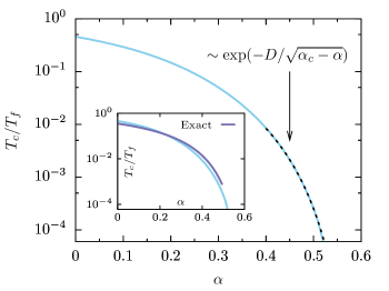
Figure 3: Superconducting transition temperature normalized by $T_{f}$ as function of the pair-breaking strength determined from the solution of the gap equation Eq.(12), in comparison BKT-scaling behavior of Eq.(1) (dashed curve) with $\alpha_{c}\approx 0.62$ and $D\approx 4.8$. Inset shows comparison of $T_{c}$ determined by solving Eq.(12) with the exact solution for $g=1$, obtained by solving the full Eliashberg equations.

In the impurity-like regime $T^{*}<T<T_{f}$ for strong coupling $g>1$, the $\alpha=0$ transition temperature approaches a constant value $T_{c}^{0}\approx 0.112\omega_{0}$. For the crossover temperature $T^{*}$ we find $T^{*}=9\omega_{0}g^{-2}/256$. As long as $T_{c}\left(\alpha\right)>T^{*}$ we can analyze the effects of pair breaking by solving the linearized gap equation and using the normal state results from the impurity-like regime:

$$\Delta\left(\epsilon_{n}\right)=\frac{3\omega_{0}^{2}}{\left(8\pi T_{c}\right)^{2}}\sum_{n^{\prime}}\frac{\left(1-\alpha\right)\frac{\Delta_{n^{\prime}}}{n^{\prime}+\frac{1}{2}}-\frac{\Delta_{n}}{n+\frac{1}{2}}}{\frac{T^{*}}{T_{c}}+\left(n-n^{\prime}\right)^{2}}{\rm sign}\left(n^{\prime}+\frac{1}{2}\right).$$ (13)

The solution of this equation is shown in Fig.4, in comparison with the full numerical solution of Eq.(9). The rapid drop of $T_{c}$ with $\alpha$ is well captured by Eq.(13). Of course, once $T<T^{*}$ Eq.(13) is no longer reliable, which we indicate by the horizontal dashed line in Fig.4. The initial drop can be understood if one performs a perturbation theory of the above matrix equation. Treating the gap equation as an eigenvalue equation and performing first-order perturbation theory in $\alpha$, ones finds that the perturbation is essentially diagonal, being dominated by the zero Matsubara frequency transfer term in $D\left(\epsilon_{n}-\epsilon_{n^{\prime}}\right)$, and hence goes as $\omega_{0}/T^{*}\sim g^{2}$. Denoting the (normalized) $\alpha=0$ solution of the gap equation by $\Delta^{0}\left(\epsilon_{n}\right)$, to first order we have

$$\frac{T_{c}\left(\alpha\right)}{T_{c}^{0}}\approx 1-\frac{4}{3\pi^{2}}\frac{\alpha g^{2}\omega_{0}}{T_{c}^{0}}\frac{\sum_{n}\frac{|\Delta^{0}_{n}|^{2}}{|2n+1|^{2}}}{\sum_{n}\frac{|\Delta^{0}_{n}|^{2}}{|2n+1|}}.$$ (14)

The $\alpha=0$ solution can easily be determined numerically, from which we obtain

$$T_{c}\left(\alpha\right)\approx T_{c}^{0}\left(1-A\leavevmode\nobreak\ \alpha g^{2}\right)+{\cal O}\left(\alpha^{2}\right),$$ (15)

with numerical coefficient $A\approx 1.07422$ close to unity. Thus, the transition temperature is significantly reduced already for $\alpha\approx\alpha^{*}$ with $\alpha^{*}\sim g^{-2}$. The reason for this behavior is the fragility of a superconducting state with reduced weight of the Bogoliubov quasiparticles, $Z_{B}\sim\frac{\omega_{0}}{T^{*}}\sim g^{-2}$. Thus, pair-breaking effects are strong when $\alpha$ becomes comparable to the weight of the Bogoliubov quasi-particles, confirming Eq.(2) given above.

In the limit of large $g$ one can even go beyond the leading contribution for small $\alpha$. To this end we split the sum in Eq.(13) into the terms with $n\neq n^{\prime}$ and $n=n^{\prime}$:

$$\Delta\left(\epsilon_{n}\right) = \frac{3\omega_{0}^{2}}{\left(8\pi T_{c}\right)^{2}}\sum_{n^{\prime}\neq n}\frac{\left(1-\alpha\right)\frac{\Delta\left(\epsilon_{n^{\prime}}\right)}{n^{\prime}+\frac{1}{2}}-\frac{\Delta\left(\epsilon_{n}\right)}{n+\frac{1}{2}}}{\frac{T^{*}}{T_{c}}+\left(n-n^{\prime}\right)^{2}}{\rm sign}\left(n^{\prime}+\frac{1}{2}\right).$$ (16)

$$- \alpha g^{2}\frac{2\omega_{0}}{\pi^{2}T_{c}}\frac{\Delta\left(\epsilon_{n}\right)}{\left|n+\frac{1}{2}\right|}$$

Both terms contain the pair-breaking strength $\alpha$. However, in the diagonal term $\alpha$ always enters in the combination $\alpha g^{2}$. As this term dominates for large $g$, one expects that $T_{c}\left(\alpha,g\right)\approx T_{c}\left(\alpha g^{2}\right)$ even beyond the leading order term in $\alpha$. This behavior is verified in Fig.4.

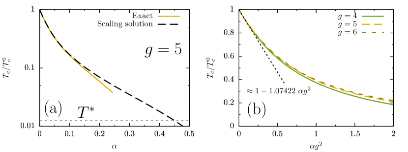
Figure 4: (a) Comparison of the transition temperature obtained using the scaling solution in the strong coupling regime, Eq.(13), with the full numerical solution for $g=5$. Dashed horizontal line is the crossover temperature $T^{*}$ below which the system enters the SYK-like regime. (b) The collapse of the transition temperature for large coupling constant $g$ is a function of $\alpha g^{2}$, with a linear slope of order unity. The data shown were obtained using the full numerical solution of the Eliashberg equation.

3.2 Analysis near $T=0$

Finally we give qualitative arguments for the behavior near the quantum critical point, including the BKT-scaling of the transition temperature near $\alpha_{c}$, Eq.(1). For $T\rightarrow 0$ the SYK power-law behavior for the bosonic and fermionic propagators properly describes the low-frequency dynamics regardless of the value of the coupling constant $g$. This allows us to use the following linearized gap equation

$$\Phi\left(\omega\right)=\frac{1-\alpha}{C_{\Delta}}\int\frac{d\omega^{\prime}}{2\pi}\frac{\Phi\left(\omega^{\prime}\right)}{\left|\omega-\omega^{\prime}\right|^{4\Delta-1}\left|\omega^{\prime}\right|^{2-4\Delta}}.$$ (17)

The constant $C_{\Delta}$ was given above.

On the one hand we need to keep in mind that the power-law behavior of this gap equation is only valid below the upper cutoff $T^{*}\approx\omega_{0}{\rm min}\left(g^{2},g^{-2}\right)$. In addition, we assume that we can use this $T=0$ gap equation to determine the transition temperature at very low $T$ if we introduce $T_{c}$ as lower cutoff. This yields:

$$\Phi\left(\omega\right)=\frac{1-\alpha}{2\pi C_{\Delta}}\int_{T_{c}}^{T^{*}}d\omega^{\prime}\left(\frac{1}{\left|\omega-\omega^{\prime}\right|^{4\Delta-1}}+\frac{1}{\left|\omega+\omega^{\prime}\right|^{4\Delta-1}}\right)\frac{\Phi\left(\omega^{\prime}\right)}{\omega^{\prime 2-4\Delta}}.$$ (18)

In our subsequent analysis of Eq.(18) we follow Ref.[15, 18, 21]. Without the upper and lower cutoffs the scale invariance of the problem suggests to look for power-law solutions $\Phi\left(\omega\right)\sim\left|\omega\right|^{-b}$. As shown in Ref.[15], the natural solutions are of the form $b=\frac{4\Delta-1}{2}\pm i\beta$, i.e. with finite imaginary part of the exponent, which yields

$$\Phi\left(\omega\right)\sim\left|\omega\right|^{-\frac{4\Delta-1}{2}}\frac{\sin\left(\beta\log\frac{T^{*}}{\left|\omega\right|}+\varphi\right)}{\sin\varphi}.$$ (19)

The phase $\varphi$ is so far arbitrary and the $\sin\varphi$ in the denominator was included for convenience. The imaginary part $\beta$ of the exponent is determined by the implicit equation $1=\frac{1-\alpha}{2\pi C_{\Delta}}J_{\Delta}(\beta)$ with

$$J_{\Delta}\left(\beta\right)=\int_{-\infty}^{\infty}dx\frac{1}{\left|1-x\right|^{4\Delta-1}\left|x\right|^{\frac{3-4\Delta}{2}+i\beta}}.$$ (20)

The integral can be evaluated explicitly, but leads to somewhat lengthy expressions. For small $\beta$ the implicit equation simplifies to $\alpha\approx\alpha_{c}-h\beta^{2}$, where $\alpha_{c}$ and $h$ depend on the exponent $\Delta$. Inserting the value $\Delta\approx 0.4203$ we find $\alpha_{c}\approx 0.626531$ and $h\approx 2.37709$. Thus, solutions with real $\beta$ exists for $\alpha<\alpha_{c}$. We will now see that this is the critical pair-breaking strength where superconductivity disappears.

The effects of the infrared and ultraviolet cutoffs can be incorporated via appropriate boundary conditions. Below $\omega=T_{c}$ the solution should be flat $\left.\frac{d\Phi\left(\omega\right)}{d\omega}\right|_{\omega=T_{c}}=0$. At the upper cut off, the natural condition for a power-law decay is that $\left.\frac{d\Phi\left(\omega\right)}{d\omega}\right|_{\omega=T^{*}}=-(4\Delta-1)\Phi\left(T^{*}\right)/T^{*}$. We will give a more detailed motivation of these conditions below. The ultraviolet boundary condition fixes the phase $\varphi$ via $\cot\varphi=\frac{4\Delta-1}{2\beta}$. The infrared boundary condition then gives the condition for the transition temperature:

$$\beta\log\left(\frac{T^{*}}{T_{c}}\right)=\pi-2\varphi.$$ (21)

One sees that $T_{c}$ vanishes when $\beta$ vanishes. Using our above result near the critical pair-breaking strength $\beta\approx h^{-1/2}\sqrt{\alpha_{c}-\alpha}$, we obtain the BKT-scaling behavior of Eq.(1) with $D=\pi\sqrt{h}\approx 4.843$. The analytic results for the critical pair-breaking strength $\alpha_{c}$ and for $D$ are in excellent agreement with our numerical results of Fig.3. The gap function right at the critical point can be obtained by taking the $\beta\rightarrow 0$ limit:

$$\Phi\left(\omega\right)\sim\left|\omega\right|^{-\frac{4\Delta-1}{2}}\left(1+\frac{4\Delta-1}{2}\log\frac{T^{*}}{\left|\omega\right|}\right).$$ (22)

The second, logarithmic term is a consequence of the boundary conditions at the upper cutoff. Right at the critical point, the overall amplitude of the gap is of course infinitesimal. The unusual frequency dependence can however be probed, at least in principle, if one measures the dynamic order-parameter susceptibility.

In order to get a better understanding of the above boundary conditions, we briefly summarize an alternative analysis that is controlled for $\Delta=1/4+\epsilon$, with small $\epsilon$. This value for the exponent does indeed occur in our model if we take the limit where the number of phonon modes $M$ is much larger than the number of fermion modes[24], in which case $\Delta=\frac{1}{4}+\sqrt{\frac{N}{8\pi M}}+\cdots$. Let us consider without loss of generality $\omega>0$. We split the integration in Eq.(18) into regimes $\omega^{\prime}<\omega$ and $\omega^{\prime}>\omega$, which we approximate as $\omega^{\prime}\ll\omega$ and $\omega^{\prime}\gg\omega$, respectively. Then it follows that

$$\Phi\left(\omega\right) \approx \frac{1-\alpha}{C_{\Delta}\omega^{4\Delta-1}}\int_{T_{c}}^{\omega}\frac{d\omega^{\prime}}{\pi}\frac{\Phi\left(\omega^{\prime}\right)}{\omega^{\prime 2-4\Delta}}+\frac{1-\alpha}{C_{\Delta}}\int_{\omega}^{\omega_{c}}\frac{d\omega^{\prime}}{\pi}\frac{\Phi\left(\omega^{\prime}\right)}{\omega^{\prime}}.$$ (23)

For $\Delta\rightarrow\frac{1}{4}$ this approximation is exact, which makes the expansion controlled for small $\epsilon$. This simplified version of the integral equation can be rewritten as a differential equation. To this end we multiply Eq.(23) with $\omega^{4\Delta-1}$, take the derivative with respect to $\omega$, multiply the result with $\omega^{2-4\Delta}$ and take once more a derivative. It follows:

$$\frac{d}{d\omega}\omega^{2-4\Delta}\frac{d}{d\omega}\omega^{4\Delta-1}\Phi\left(\omega\right)=-(1-\alpha)\frac{4\Delta-1}{\pi C_{\Delta}\omega}\Phi\left(\omega\right).$$ (24)

From the integral equation one furthermore obtains the conditions $T_{c}^{4\Delta-1}\Phi\left(T_{c}\right)=\frac{T_{c}}{4\Delta-1}\left.\frac{d\omega^{4\Delta-1}\Phi\left(\omega\right)}{d\omega}\right|_{\omega=T_{c}}$ and $\left.\frac{d\omega^{\gamma}\Phi\left(\omega\right)}{d\omega}\right|_{\omega=\omega_{c}}=0$. These are identical to the boundary conditions imposed in our above analysis. In addition, the solution of Eq.(19) solves the differential equations Eq.(24) with $\beta=\sqrt{\left(\frac{1-\alpha}{\pi C_{\Delta}}-\frac{1}{4}(4\Delta-1)\right)\left(4\Delta-1\right)}$. This yields for the critical pair-breaking strength $\alpha_{c}=\frac{1}{2}+\left(2\log 4-\pi\right)\epsilon\cdots$. We checked that this result also follows from the leading order expansion of the more general solution summarized above.

The analysis of the preceding paragraphs clearly demonstrates that the conformal symmetry of the critical normal state is lost with an energy scale that behaves according to the BKT-scaling of Eq.(1), in agreement with the general expectation of Ref.[60].

4 Summary

We introduced and solved a model of electrons that interact with phonons via a random electron-phonon coupling. The theory is a natural generalization of the Sachdev-Ye-Kitaev model to the problem of interacting electrons and phonons and gives rise to a superconductivity. Typical for fully connected models, an exact solution becomes possible in the limit $N\rightarrow\infty$. In our case this exact solution corresponds to the coupled Eliashberg equations of superconductivity. Since the normal state of the model is characterized by two non-Fermi liquid fixed points, depending on the value of the dimensionless coupling constant and temperature, the approach is an ideal toy model to study superconductivity as it emerges from a quantum critical non-Fermi liquid. In particular, a superconductor that results from a strongly incoherent normal state is characterized by a reduced weight $Z_{B}$ of the Bogoliubov quasi-particles.

The special focus of the present paper was the investigation of pair-breaking phenomena. On the one hand, we found that superconductivity disappears at a critical pair-breaking strength $\alpha_{c}$ according to BKT-scaling. This reflects the fact that the critical normal state possesses at low temperatures an emergent conformal symmetry, which is broken in the superconducting state. Thus, the way superconductivity is suppressed by pair-breaking disorder may reveal important information about the symmetry of the normal state. In addition we showed that for superconductors with small weight $Z_{B}\ll 1$ of the Bogoliubov quasiparticle, pair breaking substantially suppresses $T_{c}$ already for $\alpha\approx Z_{B}\ll\alpha_{c}$.

These results demonstrate that the formalism initially devised by Eliashberg to treat dynamical pairing phenomena in Fermi liquids with intermediate electron-phonon coupling is, in fact, general enough to address Cooper pairing in a broader class of systems, such as strongly correlated, quantum critical systems.

References

- [1] G. M. Eliashberg, Interactions between electrons and lattice vibrations in a superconductor, Sov. Phys. JETP 11, 696 (1960).
- [2] G. M. Eliashberg, Temperature Green’s functions for electrons in a superconductor, Sov. Phys. JETP 12, 1000 (1961).
- [3] A. B. Migdal, Interaction between electrons and lattice vibrations in a normal metal, Sov. Phys. JETP 7, 996 (1958).
- [4] L. P. Gorkov, On the energy spectrum of superconductors, Sov. Phys. JETP 34, 505 (1958).
- [5] Y. Nambu, Quasi-Particles and Gauge Invariance in the Theory of Superconductivity, Phys. Rev. 117, 648 (1960).
- [6] J. R. Schrieffer, D.J. Scalapino, and J.W. Wilkins, Effective tunneling density of states in superconductors, Phys. Rev. Lett. 10, 336 (1963)
- [7] D. J. Scalapino, J. R. Schrieffer, J. W. Wilkins, Strong-coupling superconductivity, Phys. Rev. 148, 263 (1966).
- [8] W. L. McMillan, Transition Temperature of Strong-Coupled Superconductors, Phys. Rev. 167, 331(1968).
- [9] D. J. Scalapino R.D. Parks (Ed.), Superconductivity, The Electron–Phonon Interaction and Strong Coupling Superconductors, Vol. 1, Dekker Inc, New York (1969), p. 449
- [10] W. L. McMillan, J. M. Rowell, M. Parks (Ed.), Superconductivity, Tunneling and Strong Coupling Superconductivity, Vol. 1, Dekker Inc, New York, p. 561 (1969).
- [11] P. B. Allen and R. C. Dynes, Transition temperature of strong-coupled superconductors reanalyzed, Phys. Rev. B 12, 905 (1975).
- [12] J. P. Carbotte, Properties of boson-exchange superconductors, Rev. Mod. Phys. 62, 1027 (1990).
- [13] N. E. Bonesteel, I. A. McDonald, and C. Nayak, Gauge Fields and Pairing in Double-Layer Composite Fermion Metals, Phys. Rev. Lett. 77, 3009 (1996).
- [14] D.T. Son, Superconductivity by long-range color magnetic interaction in high-density quark matter, Phys. Rev. D 59, 094019 (1999).
- [15] Ar. Abanov, A. Chubukov, and A. Finkel’stein, Coherent vs. incoherent pairing in 2D systems near magnetic instability, Europhys. Lett. 54, 488 (2001).
- [16] Ar. Abanov, A. V. Chubukov, and J. Schmalian, Quantum-critical superconductivity in underdoped cuprates, Europhys. Lett. 55, 369 (2001).
- [17] R. Roussev and A. J. Millis, Quantum critical effects on transition temperature of magnetically mediated p-wave superconductivity, Phys. Rev. B 63, 140504R (2001).
- [18] A. V. Chubukov and J. Schmalian, Superconductivity due to massless boson exchange in the strong-coupling limit, Phys. Rev. B 72, 174520 (2005).
- [19] M. A. Metlitski, D. F. Mross, S. Sachdev, and T. Senthil, Cooper pairing in non-Fermi liquids, Phys. Rev. B 91, 115111 (2015).
- [20] S. Raghu, G. Torroba, and H. Wang, Metallic quantum critical points with finite BCS couplings, Phys. Rev. B 92, 205104 (2015).
- [21] Y. Wang, A. Abanov, B. L. Altshuler, E. A. Yuzbashyan, and A. V. Chubukov, Superconductivity near a Quantum-Critical Point: The Special Role of the First Matsubara Frequency, Phys. Rev. Lett. 117, 157001 (2016).
- [22] A. Abanov, Y.-M. Wu, Y. Wang, and A. V. Chubukov, Superconductivity above a quantum critical point in a metal: Gap closing versus gap filling, Fermi arcs, and pseudogap behavior, Phys. Rev. B 99, 180506(R) (2019).
- [23] Y.-M. Wu, A. Abanov, Y. Wang, and A. V. Chubukov, Special role of the first Matsubara frequency for superconductivity near a quantum critical point: Nonlinear gap equation below and spectral properties in real frequencies, Phys. Rev. B 99, 144512 (2019).
- [24] I. Esterlis and J. Schmalian, Cooper pairing of incoherent electrons: An electron-phonon version of the Sachdev-Ye-Kitaev model, Phys. Rev. B 100, 115132 (2019).
- [25] S. Sachdev and J. Ye, Gapless spin liquid ground state in a random, quantum Heisenberg magnet, Phys. Rev. Lett. 70, 3339, (1993).
- [26] A. Georges, O. Parcollet, and S. Sachdev, Mean Field Theory of a Quantum Heisenberg Spin Glass, Phys. Rev. Lett. 85, 840 (2000).
- [27] S. Sachdev, Holographic Metals and the Fractionalized Fermi Liquid, Phys. Rev. Lett. 105, 151602 (2010).
- [28] A. Kitaev, Hidden correlations in the Hawking radiation and thermal noise, Talk at KITP http://online.kitp.ucsb.edu/online/joint98/kitaev/, February, 2015.
- [29] A. Kitaev, A simple model of quantum holography. Talks at KITP http://online.kitp.ucsb.edu/online/entangled15/kitaev/ and http://online.kitp.ucsb.edu/online/entangled15/kitaev2/, April and May, 2015.
- [30] A. A. Patel, M. J. Lawler, and E.-A. Kim, Coherent Superconductivity with a Large Gap Ratio from Incoherent Metals, Phys. Rev. Lett. 121, 187001 (2018).
- [31] Y. Wang, A Solvable Random Model with Quantum-critical Points for non-Fermi-liquid Pairing, arXiv:1904.07240.
- [32] D. Chowdhury and E. Berg, Intrinsic superconducting instabilities of a solvable model for an incoherent metal, arXiv:1908.02757
- [33] P. W. Anderson, Theory of dirty superconductors, J. Phys. Chem Solids 11, 26 (1959).
- [34] A. A. Abrikosov and L. P. Gor’kov, On the theory of superconducting alloys. 1. The electrodynamics of alloys at absolute zero, Zh. Eksp. Teor. Fiz. 35, 1558 (1958) ,[Sov. Phys. JETP 8, 1090 (1959)].
- [35] A. A. Abrikosov and L. P. Gor’kov, Superconducting alloys at finite temperatures, Zh. Eksp. Teor. Fiz. 36, 319 (1959) ,[Sov. Phys. JETP 9, 220 (1959)].
- [36] A. Abrikosov and L. P. Gor’kov, Contribution to the theory of superconducting alloys with paramagnetic impurities, Zh. Eksp. Teor. Fiz. 39, 1781 (1961) ,[Sov. Phys. JETP 12, 1243 (1961)].
- [37] E. Müller-Hartmann and J. Zittartz, Kondo effect in superconductors, Phys. Rev. Lett. 26, 428 (1971).
- [38] S. Yoksan and A. D. S. Nagi, Shiba-Rusinov theory of magnetic impurities in anisotropic superconductors: Eliashberg formalism, Phys. Rev. B 30, 2659 (1984).
- [39] P. Monthoux and D. Pines, Spin-fluctuation-induced superconductivity and normal-state properties of YBa2Cu3O7, Phys. Rev. B 49, 4261 (1994).
- [40] G. Preosti and P. Muzikar, Superconducting order parameters with sign changes: The density of states and impurity scattering, Phys. Rev. B 54, 3489 (1996).
- [41] A. A. Golubov and I. I. Mazin, Effect of magnetic and nonmagnetic impurities on highly anisotropic superconductivity, Phys. Rev. B 55, 15146 (1997).
- [42] M. Franz, C. Kallin, A. J. Berlinsky, and M. I. Salkola, Critical temperature and superfluid density suppression in disordered high- cuprate superconductors, Phys. Rev. B 56, 7882 (1997).
- [43] G. Harań and A. D. S. Nagi, Effect of anisotropic impurity scattering in superconductors, Phys. Rev. B 58, 12441 (1998).
- [44] M. L. Kulić and O. V. Dolgov, Anisotropic impurities in anisotropic superconductors, Phys. Rev. B 60, 13062 (1999).
- [45] M. Dzero and J. Schmalian, Superconductivity in Charge Kondo Systems, Phys. Rev. Lett. 94, 157003 (2005).
- [46] A. V. Balatsky, I. Vekhter, and J.-X. Zhu, Impurity-induced states in conventional and unconventional superconductors, Rev. Mod. Phys. 78, 373 (2006).
- [47] S. Graser, P. J. Hirschfeld, L. Y. Zhu, and T. Dahm, Tc suppression and resistivity in cuprates with out of plane defects, Phys. Rev. B 76, 054516 (2007).
- [48] H. Alloul, J. Bobroff, M. Gabay, and P. J. Hirschfeld, Defects in correlated metals and superconductors, Rev. Mod. Phys. 81, 45 (2009).
- [49] A. Kemper, D. G. S. P. Doluweera, T. A. Maier, M. Jarrell, P. J. Hirschfeld, and H. P. Cheng, Insensitivity of -wave pairing to disorder in the high-temperature cuprate superconductors, Phys. Rev. B 79, 104502 (2009).
- [50] V. G. Kogan, Pair breaking in iron pnictides, Phys. Rev. B 80, 214532 (2009).
- [51] A. B. Vorontsov, M. G. Vavilov, and A. V. Chubukov, Superfluid density and penetration depth in the iron pnictides, Phys. Rev. B 79, 140507R (2009).
- [52] A. B. Vorontsov, Ar. Abanov, M. G. Vavilov, and A. V. Chubukov, Reduced effect of impurities on the universal pairing scale in the cuprates, Phys. Rev B 81, 012508 (2010).
- [53] K. Michaeli and L. Fu, Spin-Orbit Locking as a Protection Mechanism of the Odd-Parity Superconducting State against Disorder, Phys. Rev. Lett. 109, 187003 (2012).
- [54] M. Hoyer, M. S. Scheurer, S. V. Syzranov, and J. Schmalian, Pair breaking due to orbital magnetism in iron-based superconductors, Phys. Rev. B 91, 054501 (2015).
- [55] M. S. Scheurer, M. Hoyer, and J. Schmalian, Pair breaking in multiorbital superconductors: An application to oxide interfaces, Phys. Rev. B 92, 014518, (2015).
- [56] J. Kang and R. M. Fernandes, Robustness of quantum critical pairing against disorder, Phys. Rev. B 93, 224514 (2016).
- [57] T. V. Trevisan, M. Schütt, and R. M. Fernandes, Impact of disorder on the superconducting transition temperature near a Lifshitz transition, Phys. Rev. B 98, 094514 (2018).
- [58] V. L. Berezinskii, Destruction of long range order in one-dimensional and two-dimensional systems having a continuous symmetry group. I. Classical systems, Sov. Phys. JETP, 32, 493 (1971); Sov. Phys. JETP, 34, 610 (1972).
- [59] J. M. Kosterlitz and J. D. Thouless, Ordering, metastability and phase transitions in two-dimensional systems, Journal of Physics C: Solid State Physics, 6, 1181 (1973).
- [60] D. B. Kaplan, J.-W. Lee, D. T. Son, and M. A. Stephanov, Conformality lost, Phys. Rev. D 80, 125005 (2009).
- [61] T. Appelquist, D. Nash, and L. C. R. Wijewardhana, Critical Behavior in (2+1)-Dimensional QED, Phys. Rev. Lett. 60, 2575 (1988).
- [62] M.L. Mehta, Random matrices, 3rd edition, Elsevier (2004).
- [63] S. F. Edwards and P. W. Anderson, Theory of spin glasses, J. Phys. F 5, 965 (1975).