Far-field asymptotics for multiple-pole solitons in the large-order limit

Abstract.

The integrable focusing nonlinear Schrödinger equation admits soliton solutions whose associated spectral data consist of a single pair of conjugate poles of arbitrary order. We study families of such multiple-pole solitons generated by Darboux transformations as the pole order tends to infinity. We show that in an appropriate scaling, there are four regions in the space-time plane where solutions display qualitatively distinct behaviors: an exponential-decay region, an algebraic-decay region, a non-oscillatory region, and an oscillatory region. Using the nonlinear steepest-descent method for analyzing Riemann-Hilbert problems, we compute the leading-order asymptotic behavior in the algebraic-decay, non-oscillatory, and oscillatory regions.

1. Introduction

The one-dimensional focusing cubic nonlinear Schrödinger (NLS) equation

(1.1) $$i\psi_{t}+\frac{1}{2}\psi_{xx}+|\psi|^{2}\psi=0,\quad x,t\in\mathbb{R},$$

is well known to be a completely integrable equation admitting solitons, i.e. localized traveling-wave solutions. Each initial datum from an appropriate function space (Schwartz space is sufficient for our needs) is associated with a set of scattering data, consisting of poles and norming constants encoding solitons, as well as a reflection coefficient encoding radiation. The scattering data for a standard soliton consist of a complex-conjugate pair of first-order poles (and an associated norming constant) and an identically zero reflection coefficient. However, for any $n\in\mathbb{Z}_{+}$, the NLS equation also has solutions whose scattering data consist of a complex-conjugate pair of poles order $n$ (plus $n$ auxiliary parameters that are higher-order analogues of norming constants) and no reflection. These mulitple-pole solitons ($n\geq 2$) have very different qualitative behavior than standard solitons. At sufficiently large time scales, the $n$th-order pole soliton resembles $n$ solitons approaching each other, interacting, and then separating again. This complicated interaction displays a remarkable degree of structure at different scales as $n$ increases. These distinguished scales include:

The near-field limit. The scaling $X:=nx$, $T:=n^{2}t$ is appropriate for studying the rogue-wave-type behavior near the origin. Here the key feature is a single peak with amplitude of order $n$. Locally the solution satisfies for each fixed $T$ a certain differential equation in the Painlevé-III hierarchy. This regime was analyzed by two of the authors in [1], the first large-$n$ analysis of $n$th-order pole solitons. The asymptotic solution seems to be a type of universal behavior, also appearing in the study of high-order Peregrine breathers for the NLS equation with constant, non-zero boundary conditions [2].

The far-field limit. Define

(1.2) $$\chi:=\frac{x}{n},\quad\tau:=\frac{t}{n}.$$

As the pole order $n\to\infty$, then the ($\chi$,$\tau$)-plane can be partitioned into $n$-independent regions in which the multiple-pole soliton has distinct behaviors, such as rapid oscillations of frequency $n$ or decay to zero. This scaling was previously studied in [1] and is the focus of the current work.

The long-time limit. If $x$ and $t$ are unscaled, then as $t\to{\pm}\infty$ the $n$th-order pole soliton asymptotically resembles a train of $n$ distinct one-solitons. Asymptotics as $t\to\pm\infty$ were obtained by Olmedilla in [14] for $n$th-order pole solitons for fixed order $n=2$ and $n=3$ by solving Gel’fand-Levitan-Marchenko equations with an appropriate kernel and arriving at a representation for the $n$th-order pole soliton that involves determinants of size $n$ via Cramer’s rule. Large-$t$ asymptotics for multiple-pole solutions of arbitrary but finite and fixed order $n$ were obtained by Schiebold in [18] using the earlier algebraic results [16] by the same author.

$n=2$                                     $n=4$                                     $n=8$

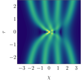
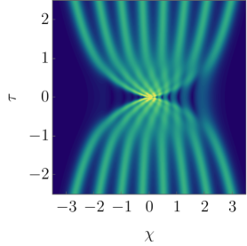
Figure 1. The far-field scaling. Plots of $|\psi^{[2n]}(n\chi,n\tau;(1,3),i)|$ for $-3.5\leq\chi\leq 3.5$ and $-2.5\leq\tau\leq 2.5$, where $\psi^{[2n]}(n\chi,n\tau;(1,3),i)$ is a multiple-pole soliton solution of the nonlinear Schrödinger equation (1.1). In each plot $c_{1}=1$, $c_{2}=3$, and $\xi=i$. Left: $n=2$, Center: $n=4$. Right: $n=8$.

The generic $n$th-order pole soliton depends on a complex parameter $\xi$ (the spectral pole in the upper half-plane) and $n$ constant nonzero row vectors $(d_{1,j},d_{2,j})\in\mathbb{C}^{2}$, $j=1,...,n$ (higher-order analogues of the norming constants). This function can be constructed via $n$ iterated Darboux transformations as described in [1, §2]. Working directly with a Riemann-Hilbert problem characterization in the context of the robust inverse-scattering transform framework provides fundamental eigenfunction matrices that are analytic at $\xi$ after each iteration by encoding the effect of the Darboux transformation in the form of a jump condition instead of a singularity in the spectral plane. In order to obtain well-defined limits as $n\to\infty$, we first fix nonzero complex numbers $c_{1}$ and $c_{2}$ and set ${\bf c}:=(c_{1},c_{2})\in(\mathbb{C}^{*})^{2}$ (here $\mathbb{C}^{*}:=\mathbb{C}\setminus\{0\}$). We then take $(d_{1,j},d_{2,j}):=(\epsilon^{-1}c_{1},\epsilon^{-1}c_{2})$ for $j=1,...,n$ and take the limit $\epsilon\to 0^{+}$. See Figure 1 for plots of representative multiple-pole solitons in the far-field scaling. This construction procedure is given in Appendix A for completeness of our work, and it yields a representation of these multiple-pole solitons $\psi^{[2n]}(x,t;{\bf c},\xi)$ given in Riemann-Hilbert Problem 1 below, which is convenient for our purposes of asymptotic analysis.

A related avenue of research pioneered by the work of Gesztesy, Karwowski, and Zhao in [10] is the so-called countable superposition of solitons. The authors considered a sequence of distinct eigenvalues $\{-\kappa_{j}^{2}\}_{j=1}^{\infty}$ along with associated norming constants $\{c_{j}\}_{j=1}^{\infty}$ and zero reflection coefficient for the Schrödinger operator. For each finite $N\in\mathbb{N}$, the scattering data $\{\kappa_{j},c_{j}\}_{j=1}^{N}$ defines a reflectionless $N$-soliton solution $V_{N}(x,t)$ of the Korteweg-de Vries equation. Under certain summability and growth conditions on $\{\kappa_{j},c_{j}\}$ as $N\to+\infty$, the authors established a limiting solution $V_{\infty}(x,t)$ of the Korteweg-de Vries equation that is reflectionless, global, and smooth. The study of countable superposition of solitons was extended to the focusing NLS equation (1.1) later by Schiebold in [15] and [17] for a sequence of distinct eigenvalues $\{\lambda_{j}\}_{j=1}^{\infty}$ of the Zakharov-Shabat problem in the upper half-plane along with the associated norming constants again subject to appropriate growth conditions. Drawing a comparison, the solutions we study can be thought of as a countable superposition as $n\to+\infty$ over $\mathbb{N}$, albeit with $\lambda_{j}\equiv\xi$ for all $j\in\mathbb{N}$. Due to the repeated choice of the exceptional points $\lambda_{j}$, however, the family of solutions we study fall outside of the classes studied in these works. Indeed, following the proof of [1, Lemma 1], it is easy to see that $\psi^{[2n]}(0,0;\mathbf{c},\xi)=8\Im(\xi)c_{1}c_{2}^{*}|\mathbf{c}|^{-2}n$, and hence the amplitudes of the solutions $\psi^{[2n]}(x,t;\mathbf{c},\xi)$ explode as $n\to+\infty$. Therefore, there is not a limiting profile in the unscaled $(x,t)$-plane as $n\to+\infty$, contrary to the case in [10, 15, 17]. On the other hand, for each $n\in\mathbb{N}$, $\psi^{[2n]}(x,t;\mathbf{c},\xi)$ defines a global classical solution (in fact, real-analytic in $(x,t)$) of the focusing NLS equation (1.1). This is a consequence of analytic Fredholm theory applied to the Riemann-Hilbert Problem 1, which has analytic dependence on $(x,t)$ with a compact jump contour (see [2, Proposition 3] for details). Regularity properties of these solutions for fixed $n\in\mathbb{N}$ were also recently established using determinant representations [19].

In the present work we show that in the far-field scaling $\psi^{[2n]}(n\chi,n\tau;{\bf c},\xi)$ has four qualitatively different behaviors depending on the values of $\chi$ and $\tau$, and we give the leading-order large-$n$ asymptotic behavior for all $\chi$ and $\tau$ off the boundary curves. As $n\to\infty$, $\psi^{[2n]}(n\chi,n\tau;{\bf c},\xi)$ exhibits the following four behaviors:

The exponential-decay region. In this region the solution decays exponentially fast to zero as $n\to\infty$. This was proven in [1]. In the Riemann-Hilbert analysis the model problem has no bands (indicating no order-one contributions) and no parametrices (indicating no algebraically decaying contributions).

The algebraic-decay region. Here the leading-order solution decays as $n^{-1/2}$ and is given explicitly in terms of elementary functions. The Riemann-Hilbert model problem consists of no bands and two parabolic-cylinder parametrices giving the leading-order contribution to the solution.

The non-oscillatory region. In this region the leading-order solution is independent of $n$ and can be written explicitly up to the solution of a septic equation. The model Riemann-Hilbert problem has a single band.

The oscillatory region. In the final region the solution exhibits rapid oscillations with frequency of order $n$ within an amplitude envelope of order one. The leading-order behavior is written in terms of genus-one Riemann-theta functions. The corresponding Riemann-Hilbert model problem has two bands.

The four far-field regions depend on $\xi$ but are independent of ${\bf c}$. The regions are illustrated for $\xi=i$ in Figure 2.

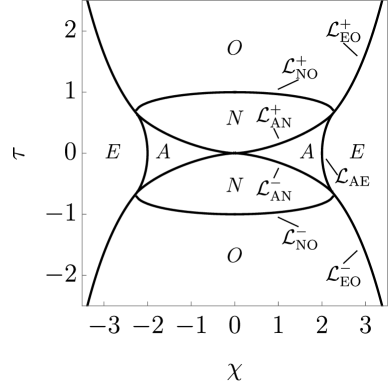
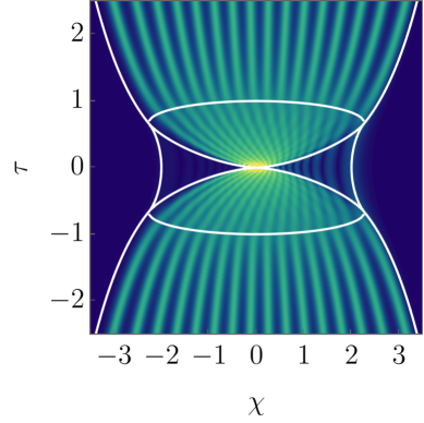
Figure 2. The boundaries of the far-field regions. Left: The algebraic-decay, exponential-decay, non-oscillatory, and oscillatory regions (denoted by A, E, N, and O, respectively), along with the various boundary curves for $\xi=i$. Right: The boundary curves superimposed on $|\psi^{[2n]}(n\chi,n\tau;(1,3),i)|$ with $c_{1}=1$, $c_{2}=3$, and $\xi=i$ for $-3.5\leq\chi\leq 3.5$ and $-2.5\leq\tau\leq 2.5$.

1.1. The far-field regions.

In order to give our exact results we start by defining the region boundaries. We write $\xi=\alpha+i\beta$, $\alpha\in\mathbb{R}$, $\beta>0$.

Definition of the boundaries of the algebraic-decay region. Define

(1.3) $$\varphi(\lambda;\chi,\tau;\xi):=i(\lambda\chi+\lambda^{2}\tau)+\log\left(\frac{\lambda-\xi^{*}}{\lambda-\xi}\right).$$

This is the controlling phase function in the exponential-decay and algebraic-decay regions. The critical points of $\varphi(\lambda)$ satisfy

(1.4) $$2\tau(\lambda-\alpha)^{3}+(\chi+2\alpha\tau)(\lambda-\alpha)^{2}+2\beta^{2}\tau(\lambda-\alpha)+(\beta^{2}\chi-2\beta+2\alpha\beta^{2}\tau)=0.$$

First, set $\tau=0$ and $0<\chi<\frac{2}{\beta}$. Then $\varphi(\lambda)$ has two real distinct critical points $\lambda^{(1)}$ and $\lambda^{(2)}$, where we choose $\lambda^{(1)}<\lambda^{(2)}$ (the third critical point is at infinity). See Figure 7. The algebraic-decay region (with $\chi>0$) consists of those $\chi$ and $\tau$ values that can be reached by continuously varying $\chi$ and $\tau$ with no two critical points coinciding. In this region if $\tau\neq 0$ then $\varphi(\lambda)$ has three distinct real critical points, which we label $\lambda^{(0)}<\lambda^{(1)}<\lambda^{(2)}$ if $\tau>0$ and $\lambda^{(1)}<\lambda^{(2)}<\lambda^{(0)}$ if $\tau<0$. The region is bounded by the locus of points in the ($\chi$,$\tau$)-plane satisfying

(1.5) $$\begin{split}&(16\alpha^{4}\beta+32\alpha^{2}\beta^{3}+16\beta^{5})\tau^{4}+(32\alpha^{3}\beta\chi-16\alpha^{3}+32\alpha\beta^{3}\chi-144\alpha\beta^{2})\tau^{3}\\ &+(24\alpha^{2}\beta\chi^{2}-24\alpha^{2}\chi+8\beta^{3}\chi^{2}-72\beta^{2}\chi+108\beta)\tau^{2}+(8\alpha\beta\chi^{3}-12\alpha\chi^{2})\tau+(\beta\chi^{4}-2\chi^{3})=0.\end{split}$$

For real $\alpha$ and positive $\beta$, this algebraic curve consists of three arcs in the ($\chi$,$\tau$)-plane that intersect pairwise at the three points

(1.6) $$P^{0}:=(0,0),\quad P^{+}:=\left(\frac{-3\sqrt{3}\alpha+9\beta}{4\beta^{2}},\frac{3\sqrt{3}}{8\beta^{2}}\right),\quad P^{-}:=\left(\frac{3\sqrt{3}\alpha+9\beta}{4\beta^{2}},\frac{-3\sqrt{3}}{8\beta^{2}}\right)$$

(each of these three points corresponds to $\lambda^{(1)}=\lambda^{(2)}=\lambda^{(0)}$). The arc with endpoints $P^{-}$ and $P^{+}$ passes through the point $\left(\frac{2}{\beta},0\right)$ on the $\chi$-axis and is denoted by $\mathcal{L}_{\text{AE}}$. This arc is a boundary between the algebraic-decay and the exponential-decay regions and corresponds to $\lambda^{(1)}=\lambda^{(2)}$. The arc from $P^{0}$ to $P^{+}$ is denoted by $\mathcal{L}_{\text{AN}}^{+}$ (and corresponds to $\lambda^{(1)}=\lambda^{(0)}$), while that from $P^{0}$ to $P^{-}$ is denoted by $\mathcal{L}_{\text{AN}}^{-}$ (and corresponds to $\lambda^{(2)}=\lambda^{(0)}$). Both of these arcs form boundaries between the algebraic-decay region and the non-oscillatory region. Note that if $\xi=i$, the defining condition (1.5) for the boundary of the algebraic-decay region simplifies to

(1.7) $$16\tau^{4}+(8\chi^{2}-72\chi+108)\tau^{2}+(\chi^{4}-2\chi^{3})=0.$$

Definition of the exponential-decay / oscillatory boundary. We now define $\mathcal{L}_{\text{EO}}^{\pm}$, the boundaries between the exponential-decay and oscillatory regions when $\chi>0$. Set $\tau=0$ and choose $\chi>\frac{2}{\beta}$. Then $\varphi(\lambda)$ has a complex-conjugate pair of critical points $\lambda^{+}$ and $\lambda^{-}$, where we choose $\lambda^{+}$ to be in the upper half-plane. See Figure 6. Here we have that $\Re(\varphi(\lambda^{\pm}))\neq 0$. The exponential-decay region consists of those $(\chi,\tau)$ pairs we can reach by continuously varying $\chi$ and $\tau$ such that no two critical points coincide and such that the level lines $\Re(\varphi(\lambda))=0$ never intersect either of the two critical points with nonzero imaginary part (which we continue to label as $\lambda^{\pm}$). In this region if $\tau\neq 0$ then there is a third finite critical point which is real and that we label as $\lambda^{(0)}$. The curve $\mathcal{L}_{\text{AE}}$ corresponds to $\lambda^{+}=\lambda^{-}$. The curve $\mathcal{L}_{\text{EO}}^{+}$ (respectively, $\mathcal{L}_{\text{EO}}^{-}$) is defined as those points with $\tau>0$ (respectively, $\tau<0$) such that $\Re(\varphi(\lambda^{+}))=\Re(\varphi(\lambda^{-}))=0$. Both $\mathcal{L}_{\text{EO}}^{+}$ and $\mathcal{L}_{\text{EO}}^{-}$ are simple, semi-infinite curves with endpoints $P^{+}$ and $P^{-}$, respectively.

Definition of the oscillatory / non-oscillatory boundary. Finally, we define $\mathcal{L}_{\text{NO}}^{+}$, the boundary between the oscillatory and non-oscillatory regions when $\tau>0$. Given a complex number $a=a(\chi,\tau)$, define

(1.8) $$R(\lambda)\equiv R(\lambda;\chi,\tau):=((\lambda-a(\chi,\tau))(\lambda-a(\chi,\tau)^{*}))^{1/2}$$

with asymptotic behavior $R(\lambda)=\lambda+\mathcal{O}(1)$ as $\lambda\to\infty$ and branch cut from $a^{*}$ to $a$ (we will completely specify the branch cut momentarily). Set

(1.9) $$g^{\prime}(\lambda):=\frac{R(\lambda)}{R(\xi^{*})(\xi^{*}-\lambda)}-\frac{R(\lambda)}{R(\xi)(\xi-\lambda)}-2i\tau R(\lambda)+i\chi+2i\tau\lambda+\frac{1}{\lambda-\xi^{*}}-\frac{1}{\lambda-\xi}.$$

Then $a(\chi,\tau)$ is chosen so that $g^{\prime}(\lambda)=\mathcal{O}(\lambda^{-2})$ as $\lambda\to\infty$. The function $\varphi^{\prime}(\lambda)-g^{\prime}(\varphi)$ (which will turn out to be the derivative of the controlling phase function in the non-oscillatory region) has two real zeros if $(\chi,\tau)\in\mathcal{L}_{\text{AN}}^{+}$. One zero is simple (corresponding to $\lambda^{(2)}$ from the algebraic-decay region) and one zero is double (corresponding to $\lambda^{(0)}=\lambda^{(1)}$ from the algebraic-decay region). See Figure 9. Keeping $\chi$ fixed and increasing $\tau$, the double zero splits into one real zero (denoted by $\lambda^{(1)}$) and two square-root branch points at $a$ and $a^{*}$. The simple real zero persists and is again denoted by $\lambda^{(2)}$. See Figure 11. We now choose the branch cut for $R(\lambda)$ (and thus the cut for $g^{\prime}(\lambda)$ as well) to run from $a^{*}$ to $\lambda^{(1)}$ to $a$. As $\chi$ increases, the non-oscillatory region continues until the two real zeros coincide: $\lambda^{(1)}=\lambda^{(2)}$. This is the condition for the contour $\mathcal{L}_{\text{NO}}$ separating the non-oscillatory and oscillatory regions.

The exponential-decay, algebraic-decay, non-oscillatory, and oscillatory regions are now defined by these boundary curves as illustrated in Figure 2.

1.2. Results.

We now give our main results, the leading-order asymptotic behavior in each of the four regions. The symmetry properties of $\psi^{[2n]}(x,t)$ stated in Proposition 1 allow us to restrict our analysis to the first quadrant of the $(\chi,\tau)$ plane without loss of generality.

Theorem 1.

(The exponential-decay region). Fix $\chi>0$ and $\tau\geq 0$ so that $(\chi,\tau)$ is in the exponential-decay region. Then

(1.10) $$\psi^{[2n]}(n\chi,n\tau)=\mathcal{O}(e^{-\delta n}),\quad{n\to+\infty},$$

for some constant $\delta>0$.

Theorem 1 was proven in [1, §3].

Theorem 2.

(The algebraic-decay region). Fix $\chi>0$ and $\tau\geq 0$ so that $(\chi,\tau)$ is in the algebraic-decay region. Let $\lambda^{(1)}$, $\lambda^{(2)}$, and $\lambda^{(0)}$ be the real critical points of $\varphi(\lambda)$ as defined in §1.1 with $\lambda^{(0)}<\lambda^{(1)}<\lambda^{(2)}$ if $\tau>0$ and $\lambda^{(1)}<\lambda^{(2)}$ (and $\lambda^{(0)}=\infty$) if $\tau=0$. Define

(1.11) $$p:=\frac{1}{2\pi}\log\left(1+\left|\frac{c_{2}}{c_{1}}\right|^{2}\right)\quad\text{and}\quad\nu:=\arg\left(\frac{c_{2}}{c_{1}}\right),$$

where $\log(\cdot)$ and $\arg(\cdot)$ each have the principal branch. Also introduce

(1.12) $$\theta(\lambda;\chi,\tau):=-i\varphi(\lambda;\chi,\tau)$$

and

(1.13) $$\phi^{[n]}(\chi,\tau):=p\log(n)+2p\log\left(\lambda^{(2)}(\chi,\tau)-\lambda^{(1)}(\chi,\tau)\right)+\frac{\pi}{4}+p\log(2)-\arg(\Gamma(ip)),$$

where $\Gamma(\cdot)$ is the standard gamma function. Then

(1.14) $$\begin{split}\psi^{[2n]}(n\chi,n\tau)=\frac{\sqrt{2p}\,e^{-i\nu}}{n^{1/2}}&\left(\frac{e^{-2i{n}\theta(\lambda^{(1)};\chi,\tau)}(-\theta^{\prime\prime}(\lambda^{(1)};\chi,\tau))^{-ip}}{\sqrt{-\theta^{\prime\prime}(\lambda^{(1)};\chi,\tau)}}e^{-i\phi^{[n]}(\chi,\tau)}\right.\\ &\hskip 14.45377pt\left.+\frac{e^{-2i{n}\theta(\lambda^{(2)};\chi,\tau)}\theta^{\prime\prime}(\lambda^{(2)};\chi,\tau)^{ip}}{\sqrt{\theta^{\prime\prime}(\lambda^{(2)};\chi,\tau)}}e^{i\phi^{[n]}(\chi,\tau)}\right)+\mathcal{O}(n^{-1}),\quad{n\to+\infty}.\end{split}$$

Theorem 2 is proven in §2. Figure 3 compares the exact solution to the leading-order behavior for various values of $n$.

$n=2$                                 $n=4$                                     $n=8$

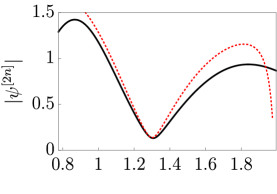
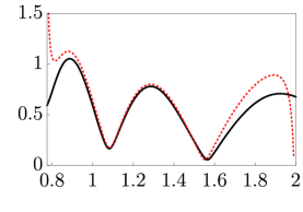
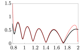
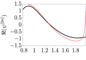
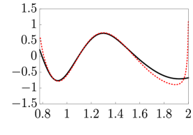
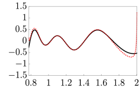
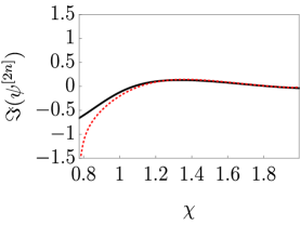
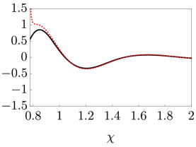
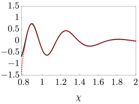
Figure 3. Convergence of the leading-order asymptotic approximation in the algebraic-decay region for $\xi=i$ and ${\bf c}=(1,3)$ at $\tau=\frac{1}{10}$. Solid black curves are for the exact solution $\psi^{[2n]}(n\chi,n\frac{1}{10};(1,3),i)$ while dashed red curves are for the leading-order approximation given by Theorem 2. For this time slice the algebraic-decay region (with $\chi\geq 0$) is approximately $0.7756<\chi<2.0050$. Left-to-right: $n=2$, $n=4$, $n=8$. Top-to-bottom: The absolute value, real part, and imaginary part.

Theorem 3.

(The non-oscillatory region). Fix $\chi\geq 0$ and $\tau>0$ so that $(\chi,\tau)$ is in the non-oscillatory region. Recall that in this region $R(\lambda)$ and $g^{\prime}(\lambda)$ are defined in (1.8) and (1.9), respectively. Let $a(\chi,\tau)$ be defined as before so that $g^{\prime}(\lambda)=\mathcal{O}(\lambda^{-2})$ as $\lambda\to\infty$, and define $K(\chi,\tau)$ by (3.28) and $f(\infty;\chi,\tau)$ by (3.40). Then

(1.15) $$\psi^{[2n]}(n\chi,n\tau)=-i\Im(a(\chi,\tau))e^{-2f(\infty;\chi,\tau)}{e^{-2inK(\chi,\tau)}}+\mathcal{O}\left(\frac{1}{n^{1/2}}\right),\quad{n\to+\infty}.$$

Theorem 3 is proven in §3. Figure 4 compares the exact solution to the leading-order behavior for various values of $n$.

$n=2$                                 $n=4$                                     $n=8$

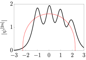
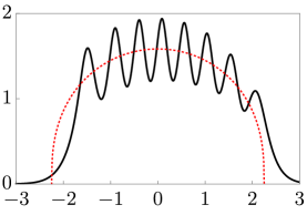
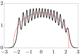
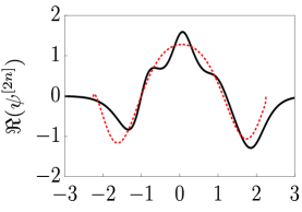
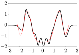
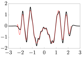
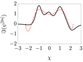
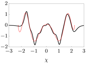
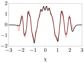
Figure 4. Convergence of the leading-order asymptotic approximation in the non-oscillatory region for $\xi=i$ and ${\bf c}=(1,3)$ at $\tau=\frac{3\sqrt{3}}{8}$. Solid black curves are for the exact solution $\psi^{[2n]}(n\chi,n\frac{3\sqrt{3}}{8};(1,3),i)$ while dashed red curves are for the leading-order approximation given by Theorem 3. For this time slice the non-oscillatory region is exactly $-\frac{9}{4}\leq\chi\leq\frac{9}{4}$. Left-to-right: $n=2$, $n=4$, $n=8$. Top-to-bottom: The absolute value, real part, and imaginary part.

Theorem 4.

(The oscillatory region). Fix $\chi\geq 0$ and $\tau>0$ so that $(\chi,\tau)$ is in the oscillatory region. Define $a\equiv a(\chi,\tau)$ and $b\equiv b(\chi,\tau)$ by (4.5), $F_{1}\equiv F_{1}(\chi,\tau)$ by (4.31), $F_{0}\equiv F_{0}(\chi,\tau)$ by (4.32), $A(\lambda)\equiv A(\lambda;\chi,\tau)$ by (4.36), $B\equiv B(\chi,\tau)$ by (4.37), $J\equiv J(\chi,\tau)$ by (4.42), $U\equiv U(\chi,\tau)$ by (4.43), and $Q\equiv Q(\chi,\tau)$ by (4.52). Introduce the genus-one Riemann-theta function

(1.16) $$\Theta(\lambda)\equiv\Theta(\lambda;B):=\sum_{k\in\mathbb{Z}}e^{k\lambda+\frac{1}{2}Bk^{2}}.$$

Then

(1.17) $$\begin{split}\psi^{[2n]}(n\chi,n\tau)=\frac{\Theta(A(\infty)-A(Q)-i\pi-\frac{B}{2}+F_{1}U)\Theta(A(\infty)+A(Q)+i\pi+\frac{B}{2})}{\Theta(A(\infty)-A(Q)-i\pi-\frac{B}{2})\Theta(A(\infty)+A(Q)+i\pi+\frac{B}{2}-F_{1}U)}\hskip 28.90755pt&\\ \times i\Im(b-a)e^{-2F_{1}J-2F_{0}}+\mathcal{O}\left(\frac{1}{n}\right),\quad{n\to+\infty}.&\end{split}$$

Theorem 4 is proven in §4. Figure 5 compares the exact solution to the leading-order behavior for various values of $n$.

$n=2$                                 $n=4$                                     $n=8$

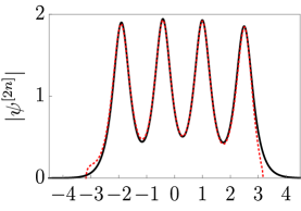
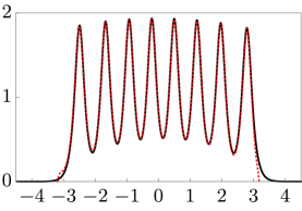
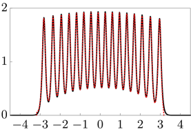
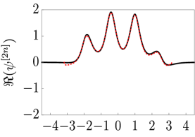
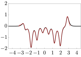
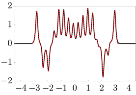
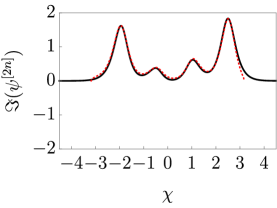
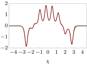
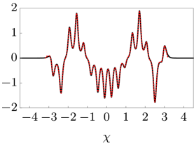
Figure 5. Convergence of the leading-order asymptotic approximation in the oscillatory region for $\xi=i$ and ${\bf c}=(1,3)$ at $\tau=2$. Solid black curves are for the exact solution $\psi^{[2n]}(n\chi,n{2};(1,3),i)$ while dashed red curves are for the leading-order approximation given by Theorem 4. For this time slice the oscillatory region is approximately $-3.178<\chi<3.178$. Left-to-right: $n=2$, $n=4$, $n=8$. Top-to-bottom: The absolute value, real part, and imaginary part.

1.3. The far-field Riemann-Hilbert problem

We now introduce the basic Riemann-Hilbert problem used to define the multiple-pole solitons we study. This representation was derived in [1] using the recently introduced robust inverse-scattering transform [3].

Riemann-Hilbert Problem 1.

(The unscaled Riemann-Hilbert problem). Fix a pole location $\xi=\alpha+i\beta\in\mathbb{C}^{+}$, a vector of connection coefficients ${\bf c}\equiv(c_{1},c_{2})\in(\mathbb{C}^{*})^{2}$, and a non-negative integer $n$. Define $D_{0}\subset\mathbb{C}$ to be a circular disk centered at the origin containing $\xi$ in its interior. Let $(x,t)\in\mathbb{R}^{2}$ be arbitrary parameters. Find the unique $2\times 2$ matrix-valued function $\mathbf{M}^{[n]}(\lambda;x,t)$ with the following properties:

• Analyticity: $\mathbf{M}^{[n]}(\lambda;x,t)$ is analytic for $\lambda\in\mathbb{C}\setminus\partial D_{0}$, and it takes continuous boundary values from the interior and exterior of $\partial D_{0}$.

• Jump condition: The boundary values on the jump contour $\partial D_{0}$ (oriented clockwise) are related as

  (1.18) $$\mathbf{M}_{+}^{[n]}(\lambda;x,t)=\mathbf{M}_{-}^{[n]}(\lambda;x,t)e^{-i(\lambda x+\lambda^{2}t)\sigma_{3}}\mathcal{S}\left(\frac{\lambda-\xi}{\lambda-\xi^{*}}\right)^{n\sigma_{3}}\mathcal{S}^{-1}e^{i(\lambda x+\lambda^{2}t)\sigma_{3}},\quad\lambda\in\partial D_{0},$$

  where

  (1.19) $$\mathcal{S}\equiv\mathcal{S}(c_{1},c_{2}):=\frac{1}{|{\bf c}|}\begin{bmatrix}c_{1}&-c_{2}^{*}\\ c_{2}&c_{1}^{*}\end{bmatrix}$$

  and $\sigma_{3}$ is the third Pauli matrix

  (1.20) $$\sigma_{3}:=\begin{bmatrix}1&0\\ 0&-1\end{bmatrix}.$$

• Normalization: $\mathbf{M}^{[n]}(\lambda;x,t)=\mathbb{I}+\mathcal{O}(\lambda^{-1})$ as $\lambda\to\infty$.

Given the solution $\mathbf{M}^{[n]}(\lambda;x,t)$, the function

(1.21) $$\psi^{[2n]}(x,t;{\bf c},\xi):=2i\lim_{\lambda\to\infty}\lambda[{\bf M}^{[n]}(\lambda;x,t;{\bf c},\xi)]_{12}$$

is a $2n^{\text{th}}$-order pole soliton solution of (1.1). We first present the following elementary symmetry properties of multiple-pole solitons of order $2n$.

Proposition 1.

Let $\mathbf{c}=(c_{1},c_{2})\in\mathbb{C}^{*}$ and $\xi=\alpha+i\beta$ with $\alpha\in\mathbb{R}$ and $\beta>0$ be given. The multiple-pole solitons $\psi^{[2n]}(x,t;(c_{1},c_{2}),\xi)$ enjoy the following symmetry properties:

(1.22) $$\psi^{[2n]}(-x,t;(c_{1},c_{2}),\xi) =\psi^{[2n]}(x,t;(-c_{2}^{*},-c_{1}^{*}),-\xi^{*}),$$

(1.23) $$\psi^{[2n]}(x,-t;(c_{1},c_{2}),\xi) =\psi^{[2n]}(x,t;(c_{1}^{*},c_{2}^{*}),-\xi^{*})^{*}.$$

A proof of based on the uniqueness of solutions of Riemann-Hilbert Problem 1 is given in Appendix B.

We analyze Riemann-Hilbert Problem 1 in the large-$n$ regime using the Deift-Zhou nonlinear steepest-descent method [9], which consists of making a series of invertible transformations in order to arrive at a problem that can be approximated in the large-$n$ limit. The first transformation introduces the far-field scaling while simplifying the form of the jump matrix. This Riemann-Hilbert problem for ${\bf N}^{[n]}(\lambda)$ will be our starting point for analysis in each of the far-field regions. Define

(1.24) $${\bf N}^{[n]}(\lambda;\chi,\tau):=\begin{cases}{\bf M}^{[n]}(\lambda;n\chi,n\tau)e^{-in(\lambda\chi+\lambda^{2}\tau)}\mathcal{S}e^{in(\lambda\chi+\lambda^{2}\tau)},&\lambda\in D_{0},\\ {\bf M}^{[n]}(\lambda;n\chi,n\tau)\left(\frac{\lambda-\xi^{*}}{\lambda-\xi}\right)^{n\sigma_{3}},&\lambda\notin D_{0}.\end{cases}$$

As $\mathbf{N}^{[n]}(\lambda;\chi,\tau)$ is related to $\mathbf{M}^{[n]}(\lambda;n\chi,n\tau)$ outside $D_{0}$ via multiplication on the right by a diagonal matrix that tends to the identity matrix as $\lambda\to\infty$, the recovery formula remains unchanged:

(1.25) $$\psi^{[2n]}(n\chi,n\tau;\mathbf{c},\xi)=2i\lim_{\lambda\rightarrow\infty}\lambda\left[\mathbf{N}^{[n]}(\lambda;\chi,\tau;\mathbf{c},\xi)\right]_{12}.$$

Riemann-Hilbert Problem 2.

(The far-field Riemann-Hilbert problem). Fix a pole location $\xi=\alpha+i\beta\in\mathbb{C}^{+}$, a vector of connection coefficients ${\bf c}\equiv(c_{1},c_{2})\in(\mathbb{C}^{*})^{2}$, and a non-negative integer $n$. Define $D_{0}\subset\mathbb{C}$ to be a circular disk centered at the origin containing $\xi$ in its interior. Let $(\chi,\tau)\in\mathbb{R}^{2}$ be arbitrary parameters. Find the unique $2\times 2$ matrix-valued function $\mathbf{N}^{[n]}(\lambda;\chi,\tau)$ with the following properties:

• Analyticity: $\mathbf{N}^{[n]}(\lambda;\chi,\tau)$ is analytic for $\lambda\in\mathbb{C}\setminus\partial D_{0}$, and it takes continuous boundary values from the interior and exterior of $\partial D_{0}$.

• Jump condition: The boundary values on the jump contour $\partial D_{0}$ (oriented clockwise) are related as ${\bf N}_{+}^{[n]}(\lambda;\chi,\tau)={\bf N}_{-}^{[n]}(\lambda;\chi,\tau){\bf V}_{\bf N}^{[n]}(\lambda;\chi,\tau)$, where

  (1.26) $${\bf V}_{\bf N}^{[n]}(\lambda;\chi,\tau):=e^{-n\varphi(\lambda;\chi,\tau)\sigma_{3}}\mathcal{S}^{-1}e^{n\varphi(\lambda;\chi,\tau)\sigma_{3}}.$$

• Normalization: $\mathbf{N}^{[n]}(\lambda;\chi,\tau)=\mathbb{I}+\mathcal{O}(\lambda^{-1})$ as $\lambda\to\infty$.

With Proposition 1 at hand, we restrict our attention to the first quadrant of the $(x,t)$-plane, hence that of the $(\chi,\tau)$-plane, for the remainder of this paper.

2. The algebraic-decay region

Pick $(\chi,\tau)$ in the algebraic-decay region. Our first objective is to understand the signature chart of $\Re(\varphi(\lambda;\chi,\tau))$.

Lemma 1.

In the algebraic-decay region, there is a domain $D_{\rm up}$ in the upper half-plane with the following properties:

• $D_{\rm up}$ contains $\xi$, is bounded by curves along which $\Re(\varphi(\lambda))=0$, and abuts the real axis along a single interval (denoted $(\lambda^{(1)},\lambda^{(2)})$).

• $\Re(\varphi(\lambda))>0$ for all $\lambda\in D_{\rm up}$.

• $\Re(\varphi(\lambda))<0$ for all $\lambda$ in the upper half-plane in the complement of $\overline{D_{\rm up}}$ but sufficiently close to $D_{\rm up}$.

Similarly, there is a domain $D_{\rm down}$ in the lower half-plane such that:

• $D_{\rm down}$ contains $\xi^{*}$, is bounded by curves along which $\Re(\varphi(\lambda))=0$, and abuts the real axis along the same interval as $D$.

• $\Re(\varphi(\lambda))<0$ for all $\lambda\in D_{\rm down}$.

• $\Re(\varphi(\lambda))>0$ for all $\lambda$ in the lower half-plane in the complement of $\overline{D_{\rm down}}$ but sufficiently close to $D_{\rm down}$.

Proof.

It is instructive to compare with the signature chart in the exponential-decay region. In [1] it was proven that in the exponential-decay region there is a closed loop in the $\lambda$-plane surrounding $\xi$ on which $\Re(\varphi(\lambda))=0$. Inside this curve $\Re(\varphi(\lambda))>0$, while outside the curve for $\lambda$ sufficiently close to the curve $\Re(\varphi(\lambda))<0$. In the lower half-plane the signature chart is symmetric with the signs flipped. If $\tau=0$ there are two critical points $\lambda^{+}$ and $\lambda^{-}$ that are complex conjugates; if $\tau\neq 0$ there is an additional real critical point $\lambda^{(0)}$. See Figure 6.

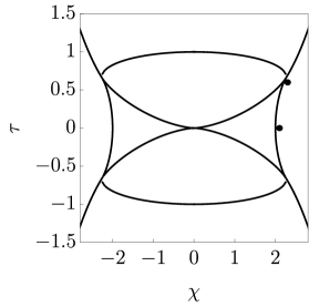
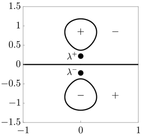
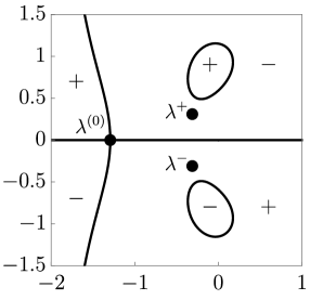
Figure 6. Signature charts of $\Re(\varphi(\lambda;\chi,\tau))$ for $\xi=i$ in the exponential-decay region, along with the critical points $\lambda^{+}$ and $\lambda^{-}$ (and, when it exists, $\lambda^{(0)}$). Left: Positions in the ($\chi$,$\tau$)-plane relative to the boundary curves. Center: $\chi=2.1$, $\tau=0$. Right: $\chi=2.3$, $\tau=0.6$.

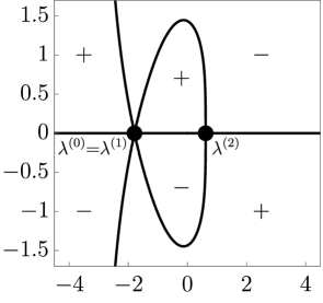
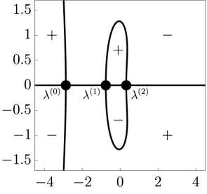
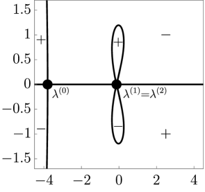
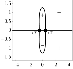
Figure 7. Signature charts of $\Re(\varphi(\lambda;\chi,\tau))$ for $\xi=i$ in the algebraic-decay region, along with the critical points $\lambda^{(1)}$ and $\lambda^{(2)}$ (and, when it exists, $\lambda^{(0)}$). Top left: $\chi=1.2$, $\tau\approx 0.2023$. Top middle: $\chi=1.65$, $\tau=0.25$. Top right: $\chi\approx 2.03$, $\tau=0.25$. Bottom left: Positions in the ($\chi$,$\tau$)-plane relative to the boundary curves. Bottom middle: $\chi=1.65$, $\tau=0$. Bottom right: $\chi=2$, $\tau=0$.

Passing from the exponential-decay region to the algebraic-decay region, the boundary curve $\mathcal{L}_{\text{AE}}$ is marked by the condition $\lambda^{+}=\lambda^{-}$. When these two critical points coincide they are real, and thus lie on a zero-level curve of $\Re(\varphi(\lambda))$. This means that the two closed curves surrounding $\xi$ and $\xi^{*}$ along which $\Re(\varphi(\lambda))=0$ must intersect at $\lambda^{+}=\lambda^{-}$ for $(\chi,\tau)$ on $\mathcal{L}_{\text{AE}}$. In the notation used in the algebraic-decay region the double critical point is $\lambda^{(1)}=\lambda^{(2)}$. See the top right and bottom right panels in Figure 7.

Now, as $(\chi,\tau)$ moves into the algebraic-decay region from $\mathcal{L}_{\text{AE}}$, the double critical point splits into the two real critical points $\lambda^{(1)}$ and $\lambda^{(2)}$. By definition, no critical points coincide inside the algebraic-decay region. In particular, this means that in the algebraic-decay region there is a domain $D_{\rm up}$ in the upper half-plane that contains $\xi$, abuts the real axis along the interval $(\lambda^{(1)},\lambda^{(2)})$, and is bounded by curves along which $\Re(\varphi(\lambda))=0$. Furthermore, $\Re(\varphi(\lambda))>0$ for all $\lambda\in D_{\rm up}$, and $\Re(\varphi(\lambda))<0$ for all $\lambda$ in the upper half-plane sufficiently close to $D_{\rm up}$. There is an analogous domain $D_{\rm down}$ in the lower half-plane containing $\xi^{*}$ such that $\Re(\varphi(\lambda))<0$ for all $\lambda\in D_{\rm down}$, and $\Re(\varphi(\lambda))>0$ for all $\lambda$ in the lower half-plane sufficiently close to $D_{\rm down}$. See the top middle and bottom middle panels in Figure 7. ∎

Define the domain $D$ to be the union of $D_{\rm up}$, $D_{\rm down}$, and the interval $(\lambda^{(1)},\lambda^{(2)})$, so that $\partial D$ is a simple Jordan curve passing through $\lambda^{(1)}$ and $\lambda^{(2)}$ along which $\Re(\varphi(\lambda))=0$. We write $\Gamma_{\text{up}}$ for the portion of $\partial D$ in the upper half-plane and $\Gamma_{\text{down}}$ for the portion of $\partial D$ in the lower half-plane. See Figure 8. We are now ready to carry out our first Riemann-Hilbert transformation, which will deform the jump contour from $\partial D_{0}$ to $\Gamma_{\text{up}}\cup\Gamma_{\text{down}}$. Set

(2.1) $${\bf O}^{[n]}(\lambda;\chi,\tau):=\begin{cases}{\bf N}^{[n]}(\lambda;\chi,\tau){\bf V}_{\bf N}^{[n]}(\lambda;\chi,\tau),&\lambda\in D_{0}\cap D^{\mathsf{c}},\\ {\bf N}^{[n]}(\lambda;\chi,\tau){\bf V}_{\bf N}^{[n]}(\lambda;\chi,\tau)^{-1},&\lambda\in D_{0}^{\mathsf{c}}\cap D,\\ {\bf N}^{[n]}(\lambda;\chi,\tau),&\text{otherwise}.\end{cases}$$

Then, orienting $\Gamma_{\text{up}}\cup\Gamma_{\text{down}}$ clockwise, the function ${\bf O}^{[n]}(\lambda)$ satisfies exactly the same Riemann-Hilbert problem as ${\bf N}^{[n]}(\lambda)$ with $\partial D_{0}$ replaced by $\Gamma_{\text{up}}\cup\Gamma_{\text{down}}$. Note that the matrix $\mathcal{S}^{-1}$ has the following two factorizations:

(2.2) $$\begin{split}\mathcal{S}^{-1}&=\begin{bmatrix}1&\frac{c_{2}^{*}}{c_{1}}\\ 0&1\end{bmatrix}\begin{bmatrix}\frac{|{\bf c}|}{c_{1}}&0\\ 0&\frac{c_{1}}{|{\bf c}|}\end{bmatrix}\begin{bmatrix}1&0\\ -\frac{c_{2}}{c_{1}}&1\end{bmatrix}\quad\quad(\text{use for }\lambda\in\Gamma_{\text{up}}),\\ \mathcal{S}^{-1}&=\begin{bmatrix}1&0\\ -\frac{c_{2}}{c_{1}^{*}}&1\end{bmatrix}\begin{bmatrix}\frac{c_{1}^{*}}{|{\bf c}|}&0\\ 0&\frac{|{\bf c}|}{c_{1}^{*}}\end{bmatrix}\begin{bmatrix}1&\frac{c_{2}^{*}}{c_{1}^{*}}\\ 0&1\end{bmatrix}\quad\quad(\text{use for }\lambda\in\Gamma_{\text{down}}).\end{split}$$

Following the exponential-decay region analysis in [1], we define the following four contours:

• $\Gamma_{\text{up}}^{\text{out}}$ runs from $\lambda^{(1)}$ to $\lambda^{(2)}$ in the upper half-plane entirely in the region where $\Re(\varphi(\lambda))<0$.

• $\Gamma_{\text{up}}^{\text{in}}$ runs from $\lambda^{(1)}$ to $\lambda^{(2)}$ entirely in $D_{\rm up}$ (so $\Re(\varphi(\lambda))>0$), and can be deformed to $\Gamma_{\text{up}}$ without passing through $\xi$.

• $\Gamma_{\text{down}}^{\text{out}}$ runs from $\lambda^{(2)}$ to $\lambda^{(1)}$ in the lower half-plane entirely in the region where $\Re(\varphi(\lambda))>0$.

• $\Gamma_{\text{down}}^{\text{in}}$ runs from $\lambda^{(1)}$ to $\lambda^{(2)}$ entirely in $D_{\rm down}$ (so $\Re(\varphi(\lambda))<0$), and can be deformed to $\Gamma_{\text{down}}$ without passing through $\xi^{*}$.

We also write

(2.3) $$\Gamma_{\text{lens}}:=\Gamma_{\text{up}}^{\text{out}}\cup\Gamma_{\text{up}}^{\text{in}}\cup\Gamma_{\text{down}}^{\text{out}}\cup\Gamma_{\text{down}}^{\text{in}}\quad\text{and}\quad\Gamma:=\Gamma_{\text{up}}\cup\Gamma_{\text{down}}\cup\Gamma_{\text{lens}}.$$

We next define the following four domains:

• $L_{\text{up}}^{\text{out}}$ is the domain in the upper half-plane bounded by $\Gamma_{\text{up}}^{\text{out}}$ and $\partial D$.

• $L_{\text{up}}^{\text{in}}$ is the domain in the upper half-plane bounded by $\Gamma_{\text{up}}^{\text{in}}$ and $\partial D$.

• $L_{\text{down}}^{\text{out}}$ is the domain in the lower half-plane bounded by $\Gamma_{\text{down}}^{\text{out}}$ and $\partial D$.

• $L_{\text{down}}^{\text{in}}$ is the domain in the lower half-plane bounded by $\Gamma_{\text{down}}^{\text{in}}$ and $\partial D$.

See Figure 8.

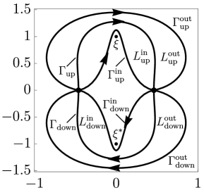
Figure 8. The lenses and lens boundaries in the algebraic-decay region.

Using these lenses, we make the change of variables

(2.4) $${\bf Q}^{[n]}(\lambda;\chi,\tau):=\begin{cases}{\bf O}^{[n]}(\lambda;\chi,\tau)\begin{bmatrix}1&\frac{c_{2}^{*}}{c_{1}}e^{-2n\varphi(\lambda;\chi,\tau)}\\ 0&1\end{bmatrix},&\lambda\in L_{\text{up}}^{\text{in}},\\ {\bf O}^{[n]}(\lambda;\chi,\tau)\begin{bmatrix}1&0\\ -\frac{c_{2}}{c_{1}}e^{2n\varphi(\lambda;\chi,\tau)}&1\end{bmatrix}^{-1},&\lambda\in L_{\text{up}}^{\text{out}},\vspace{.025in}\\ {\bf O}^{[n]}(\lambda;\chi,\tau)\begin{bmatrix}1&0\\ -\frac{c_{2}}{c_{1}^{*}}e^{2n\varphi(\lambda;\chi,\tau)}&1\end{bmatrix},&\lambda\in L_{\text{down}}^{\text{in}},\\ {\bf O}^{[n]}(\lambda;\chi,\tau)\begin{bmatrix}1&\frac{c_{2}^{*}}{c_{1}^{*}}e^{-2n\varphi(\lambda;\chi,\tau)}\\ 0&1\end{bmatrix}^{-1},&\lambda\in L_{\text{down}}^{\text{out}},\\ {\bf O}^{[n]}(\lambda;\chi,\tau),&\text{otherwise}.\end{cases}$$

Then $\mathbf{Q}^{[n]}(\lambda;\chi,\tau)$ is analytic for $\lambda\notin\Gamma$, has the normalization $\mathbf{Q}^{[n]}(\lambda;\chi,\tau)=\mathbb{I}+\mathcal{O}\left(\lambda^{-1}\right)$ as $\lambda\rightarrow\infty$, and satisfies the jump condition $\mathbf{Q}_{+}^{[n]}(\lambda;\chi,\tau)=\mathbf{Q}_{-}^{[n]}(\lambda;\chi,\tau)\mathbf{V}_{\mathbf{Q}}^{[n]}(\lambda;\chi,\tau)$ for $\lambda\in\Gamma$, where

(2.5) $$\mathbf{V}_{\mathbf{Q}}^{[n]}(\lambda;\chi,\tau):=\begin{cases}\begin{bmatrix}1&\frac{c_{2}^{*}}{c_{1}}e^{-2n\varphi(\lambda;\chi,\tau)}\\ 0&1\end{bmatrix},&\lambda\in\Gamma_{\text{up}}^{\text{in}}\,,\vspace{.025in}\\ \begin{bmatrix}\frac{|\mathbf{c}|}{c_{1}}&0\\ 0&\frac{c_{1}}{|\mathbf{c}|}\end{bmatrix},&\lambda\in\Gamma_{\text{up}}\,,\vspace{.025in}\\ \begin{bmatrix}1&0\\ -\frac{c_{2}}{c_{1}}e^{2n\varphi(\lambda;\chi,\tau)}&1\end{bmatrix},&\lambda\in\Gamma_{\text{up}}^{\text{out}}\,,\vspace{.025in}\\ \begin{bmatrix}1&0\\ -\frac{c_{2}}{c_{1}^{*}}e^{2n\varphi(\lambda;\chi,\tau)}&1\end{bmatrix},&\lambda\in\Gamma_{\text{down}}^{\text{in}}\,,\\ \begin{bmatrix}\frac{c_{1}^{*}}{|\mathbf{c}|}&0\\ 0&\frac{|\mathbf{c}|}{c_{1}^{*}}\end{bmatrix},&\lambda\in\Gamma_{\text{down}}\,,\\ \begin{bmatrix}1&\frac{c_{2}^{*}}{c_{1}^{*}}e^{-2n\varphi(\lambda;\chi,\tau)}\\ 0&1\end{bmatrix},&\lambda\in\Gamma_{\text{down}}^{\text{out}}\,.\\ \end{cases}$$

We perform the following sectionally analytic substitutions to eliminate the jump matrices supported on $\Gamma_{\text{up}}$ and $\Gamma_{\text{down}}$ at the expense of introducing a jump discontinuity across the interval

(2.6) $$I:=[\lambda^{(1)},\lambda^{(2)}]\subset\mathbb{R}$$

separating the regions $D_{\xi}$ and $D_{\xi^{*}}$:

(2.7) $$\mathbf{R}^{[n]}(\lambda;\chi,\tau):=\begin{cases}\mathbf{Q}^{[n]}(\lambda;\chi,\tau)\begin{bmatrix}\frac{|\mathbf{c}|}{c_{1}}&0\\ 0&\frac{c_{1}}{|\mathbf{c}|}\end{bmatrix},&\lambda\in D_{\text{up}}\setminus\Gamma_{\text{up}}^{\text{in}}\,,\\ \mathbf{Q}^{[n]}(\lambda;\chi,\tau)\begin{bmatrix}\frac{c_{1}^{*}}{|\mathbf{c}|}&0\\ 0&\frac{|\mathbf{c}|}{c_{1}^{*}}\end{bmatrix},&\lambda\in D_{\text{down}}\setminus\Gamma_{\text{down}}^{\text{in}}\,,\\ \mathbf{Q}^{[n]}(\lambda;\chi,\tau),&\text{otherwise}.\end{cases}$$

This substitution preserves the normalization $\mathbf{R}^{[n]}(\lambda)=\mathbb{I}+\mathcal{O}\left(\lambda^{-1}\right)$ as $\lambda\rightarrow\infty$ and $\mathbf{R}^{[n]}(\lambda)$ is analytic for $\lambda\notin\Gamma\cup I$. We orient $I$ from $\lambda^{(1)}$ to $\lambda^{(2)}$. Then $\mathbf{R}^{[n]}(\lambda)$ satisfies the jump condition $\mathbf{R}_{+}^{[n]}(\lambda;\chi,\tau)=\mathbf{R}_{-}^{[n]}(\lambda;\chi,\tau)\mathbf{V}_{\mathbf{R}}^{[n]}(\lambda;\chi,\tau)$ for $\lambda\in\Gamma\cup I$, where

(2.8) $$\mathbf{V}_{\mathbf{R}}^{[n]}(\lambda;\chi,\tau):=\begin{cases}\begin{bmatrix}1&\frac{c_{1}c_{2}^{*}}{|\mathbf{c}|^{2}}e^{-2n\varphi(\lambda;\chi,\tau)}\\ 0&1\end{bmatrix},&\lambda\in\Gamma_{\text{up}}^{\text{in}}\,,\vspace{.025in}\\ \begin{bmatrix}1&0\\ -\frac{c_{2}}{c_{1}}e^{2n\varphi(\lambda;\chi,\tau)}&1\end{bmatrix},&\lambda\in\Gamma_{\text{up}}^{\text{out}}\,,\vspace{.025in}\\ \begin{bmatrix}1&0\\ -\frac{c_{1}^{*}c_{2}}{|\mathbf{c}|^{2}}e^{2n\varphi(\lambda;\chi,\tau)}&1\end{bmatrix},&\lambda\in\Gamma_{\text{down}}^{\text{in}}\,,\vspace{.025in}\\ \begin{bmatrix}1&\frac{c_{2}^{*}}{c_{1}^{*}}e^{-2n\varphi(\lambda;\chi,\tau)}\\ 0&1\end{bmatrix},&\lambda\in\Gamma_{\text{down}}^{\text{out}}\,,\\ \begin{bmatrix}\frac{|\mathbf{c}|^{2}}{|c_{1}|^{2}}&0\\ 0&\frac{|c_{1}|^{2}}{|\mathbf{c}|^{2}}\end{bmatrix},&\lambda\in I.\end{cases}$$

This piecewise analytic transformation also preserves the recovery formula

(2.9) $$\psi^{[2n]}(n\chi,n\tau)=2i\lim_{\lambda\to\infty}\lambda[{\bf R}^{[n]}(\lambda;\chi,\tau)]_{12}.$$

Some algebraic manipulations of the jump matrix are now in order. First, we recall $\theta(\lambda;\chi,\tau):=-i\varphi(\lambda;\chi,\tau)$ from (1.12) and then note that the elements of the diagonal jump matrix supported on $I$ satisfy

(2.10) $$\frac{|\mathbf{c}|^{2}}{|c_{1}|^{2}}=1+\left\lvert\frac{c_{2}}{c_{1}}\right\rvert^{2}=e^{2\pi p},\quad p:=\frac{1}{2\pi}\log\left(1+\left\lvert\frac{c_{2}}{c_{1}}\right\rvert^{2}\right)>0.$$

Now, set

(2.11) $$\kappa:=\left\lvert\frac{c_{2}}{c_{1}}\right\rvert>0,\quad\nu:=\arg\left(\frac{c_{2}}{c_{1}}\right),$$

where $\arg(\cdot)$ denotes the principal branch, and observe that

(2.12) $$\frac{c_{1}c_{2}^{*}}{|\mathbf{c}|^{2}}=\frac{c_{2}^{*}}{c_{1}^{*}}\frac{|c_{1}|^{2}}{|\mathbf{c}|^{2}}=\kappa e^{-i\nu}e^{-2\pi p}.$$

Thus, we can rewrite the jump matrix (2.8) as

(2.13) $$\mathbf{V}_{\mathbf{R}}^{[n]}(\lambda;\chi,\tau)=\begin{cases}\begin{bmatrix}1&\kappa e^{-i\nu}e^{-2\pi p}e^{-2in\theta(\lambda;\chi,\tau)}\\ 0&1\end{bmatrix},&\lambda\in\Gamma_{\text{up}}^{\text{in}}\,,\vspace{.025in}\\ \begin{bmatrix}1&0\\ -\kappa e^{i\nu}e^{2in\theta(\lambda;\chi,\tau)}&1\end{bmatrix},&\lambda\in\Gamma_{\text{up}}^{\text{out}}\,,\vspace{.025in}\\ \begin{bmatrix}1&0\\ -\kappa e^{i\nu}e^{-2\pi p}e^{2in\theta(\lambda;\chi,\tau)}&1\end{bmatrix},&\lambda\in\Gamma_{\text{down}}^{\text{in}}\,,\vspace{.025in}\\ \begin{bmatrix}1&\kappa e^{-i\nu}e^{-2in\theta(\lambda;\chi,\tau)}\\ 0&1\end{bmatrix},&\lambda\in\Gamma_{\text{down}}^{\text{out}}\,,\\ e^{2\pi p\sigma_{3}},&\lambda\in I.\end{cases}$$

By Lemma 1, all of the jump matrices except for the diagonal jump matrix $e^{2\pi p\sigma_{3}}$ supported on $I$ decay exponentially fast to the identity matrix as $n\to\infty$ away from the critical points $\lambda^{(1)}$ and $\lambda^{(2)}$. The asymptotic analysis now closely follows [2, §4.1].

Parametrix Construction

We eliminate the constant jump condition on $I$ and deal with the non-uniform decay near the points $\lambda^{(1)}$ and $\lambda^{(2)}$ with the aid of a global parametrix $\mathbf{T}^{[n]}(\lambda)$. First, define an outer parametrix by

(2.14) $$\mathbf{T}^{(\infty)}(\lambda;\chi,\tau):=\left(\frac{\lambda-\lambda^{(1)}(\chi,\tau)}{\lambda-\lambda^{(2)}(\chi,\tau)}\right)^{ip\sigma_{3}},$$

where the powers $\pm ip$ are taken as the principal branch so that the locus where $(\lambda-\lambda^{(1)})(\lambda-\lambda^{(2)})^{-1}$ is negative coincides with the interval $I$. It is clear that $\mathbf{T}^{(\infty)}(\lambda;\chi,\tau)=\mathbb{I}+\mathcal{O}(\lambda^{-1})$ as $\lambda\to\infty$ and it can be easily verified that $\mathbf{T}^{(\infty)}(\lambda;\chi,\tau)$ is analytic for $\lambda$ in $\mathbb{C}\setminus I$, satisfying the jump condition

(2.15) $$\mathbf{T}^{(\infty)}_{+}(\lambda;\chi,\tau)=\mathbf{T}^{(\infty)}_{-}(\lambda;\chi,\tau)e^{2\pi p\sigma_{3}},\quad\lambda\in I.$$

We now move onto constructing inner parametrices that will satisfy the jump conditions exactly in small, $n$-independent disks $\mathbb{D}^{(1)}$ and $\mathbb{D}^{(2)}$ centered at $\lambda^{(1)}$ and $\lambda^{(2)}$, respectively. Before proceeding, we note that

(2.16) $$\theta^{\prime\prime}(\lambda^{(1)};\chi,\tau)<0\quad\text{and}\quad\theta^{\prime\prime}(\lambda^{(2)};\chi,\tau)>0$$

for $(\chi,\tau)$ in the algebraic-decay region. To see this, recall from §1.1 that the interval $0<\chi<\frac{2}{\beta}$ with $\tau=0$ is always contained in the algebraic-decay region. Direct calculation shows that

(2.17) $$\theta^{\prime}(\lambda;\chi,0)=\frac{\chi(\lambda-\alpha)^{2}+\beta^{2}\chi-2\beta}{(\lambda-\alpha)^{2}+\beta^{2}},\quad\theta^{\prime\prime}(\lambda;\chi,0)=\frac{4\beta(\lambda-\alpha)}{(\alpha^{2}+\beta^{2}-2\alpha\lambda+\lambda^{2})^{2}}$$

(recall $\xi=\alpha+i\beta$). From the first equation it is immediate that $\lambda^{(1)}<0<\lambda^{(2)}$ for $\tau=0$ since $0<\chi<\frac{2}{\beta}$. Then the second equation shows that $\theta^{\prime\prime}(\lambda)<0$ whenever $\lambda<\alpha$ (and so, in particular, $\theta^{\prime\prime}(\lambda^{(1)})<0$) and that $\theta^{\prime\prime}(\lambda)>0$ whenever $\lambda>\alpha$ (and so, in particular, $\theta^{\prime\prime}(\lambda^{(2)})>0$). Now $\theta(\lambda;\chi,\tau)$ is continuous for real $\lambda$, $\chi$, and $\tau$ (with the exception of an additive jump of $2\pi i$ across the logarithmic branch cut), and thus the only way the concavity at the critical points can change is if two critical points coincide. However, this condition is exactly the boundary of the algebraic-decay region, and thus (2.16) holds true everywhere in the algebraic-decay region.

Now, recalling that $\theta^{\prime}(\lambda^{(1)};\chi,\tau)=0$ and $\theta^{\prime}(\lambda^{(2)};\chi,\tau)=0$, we define the conformal mappings $f_{1}(\lambda;\chi,\tau)$ and $f_{2}(\lambda;\chi,\tau)$ locally near $\lambda=\lambda^{(1)}$ and $\lambda=\lambda^{(2)}$, respectively, by

(2.18) $$f_{1}(\lambda;\chi,\tau)^{2}:=2(\theta(\lambda^{(1)};\chi,\tau)-\theta(\lambda;\chi,\tau))\quad\text{and}\quad f_{2}(\lambda;\chi,\tau)^{2}:=2(\theta(\lambda;\chi,\tau)-\theta(\lambda^{(2)};\chi,\tau)),$$

where we choose the solutions satisfying $f_{1}^{\prime}(\lambda^{(1)};\chi,\tau)<0$ and $f_{2}^{\prime}(\lambda^{(2)};\chi,\tau)>0$. Now introducing the rescaled conformal coordinates

(2.19) $$\zeta_{1}:=n^{1/2}f_{1}(\lambda;\chi,\tau),\quad\zeta_{2}:=n^{1/2}f_{2}(\lambda;\chi,\tau)$$

and taking the rotation by $\pi$ performed by $f_{1}$ into account, the jump conditions satisfied by

(2.20) $$\mathbf{U}^{(1)}(\lambda;\chi,\tau):=\mathbf{R}^{[n]}(\lambda;\chi,\tau)e^{-in\theta(\lambda^{(1)};\chi,\tau)\sigma_{3}}e^{-i\nu\sigma_{3}/2}\begin{bmatrix}0&1\\ -1&0\end{bmatrix},\quad\lambda\in\mathbb{D}^{(1)}$$

and by

(2.21) $$\mathbf{U}^{(2)}(\lambda;\chi,\tau):=\mathbf{R}^{[n]}(\lambda;\chi,\tau)e^{-in\theta(\lambda^{(2)};\chi,\tau)\sigma_{3}}e^{-i\nu\sigma_{3}/2},\quad\lambda\in\mathbb{D}^{(2)}$$

have the same form when expressed in terms of the respective conformal coordinates $\zeta=\zeta_{1}$ and $\zeta=\zeta_{2}$ and when the jump contours are locally taken to be the rays $\arg(\zeta)=\pm\pi/4$, $\arg(\zeta)=\pm 3\pi/4$, and $\arg(-\zeta)=0$. Moreover, the resulting jump conditions coincide precisely with those in Riemann-Hilbert Problem A.1 for a parabolic cylinder parametrix in [12, Appendix A]. See Figure 9 in [12] for the relevant jump contours and matrices. Note that the condition $\kappa^{2}=e^{2\pi p}-1$ for consistency of jump conditions at $\zeta=0$ holds. We now let $\mathbf{U}(\zeta)$ denote the unique solution of the Riemann-Hilbert Problem A.1 in [12, Appendix A]. Here $\mathbf{U}(\zeta)$ is analytic for $\zeta$ in the five sectors $|\arg(\zeta)|<\frac{1}{4}\pi$, $\frac{1}{4}\pi<\arg(\zeta)<\frac{3}{4}\pi$, $-\frac{3}{4}\pi<\arg(\zeta)<-\frac{1}{4}\pi$, $\frac{3}{4}\pi<\arg(\zeta)<\pi$, and $-\pi<\arg(\zeta)<-\frac{3}{4}\pi$. It takes continuous boundary values on the excluded rays and at the origin from each sector. Furthermore, $\mathbf{U}(\zeta)\zeta^{ip\sigma_{3}}=\mathbb{I}+\mathcal{O}(\zeta^{-1})$ as $\zeta\rightarrow\infty$ uniformly in all directions and from each sector. We also have that $\mathbf{U}(\zeta)\zeta^{ip\sigma_{3}}$ has a complete asymptotic series expansion in descending integer powers of $\zeta$ as $\zeta\to\infty$, with all coefficients being independent of the sector in which $\zeta\to\infty$ [12, Appendix A.1]. In more detail, as given in (A.9) in [12], we have

(2.22) $$\mathbf{U}(\zeta)\zeta^{ip\sigma_{3}}=\mathbb{I}+\frac{1}{2i\zeta}\begin{bmatrix}0&r(p,\kappa)\\ -q(p,\kappa)&0\end{bmatrix}+\begin{bmatrix}\mathcal{O}(\zeta^{-2})&\mathcal{O}(\zeta^{-3})\\ \mathcal{O}(\zeta^{-3})&\mathcal{O}(\zeta^{-2})\end{bmatrix},\quad\zeta\to\infty,$$

where

(2.23) $$r(p,\kappa):=2e^{i\pi/4}\sqrt{\pi}\frac{e^{\pi p/2}e^{ip\ln(2)}}{\kappa\Gamma(ip)},\quad q(p,\kappa):=-\frac{2p}{r(p,\kappa)}.$$

We introduce the inner parametrices $\mathbf{T}^{(1)}(\lambda)$ and $\mathbf{T}^{(2)}(\lambda)$ by

(2.24) $$\mathbf{T}^{(1)}(\lambda;\chi,\tau):=\mathbf{Y}^{(1)}(\lambda;\chi,\tau)\mathbf{U}(n^{1/2}f_{1}(\lambda;\chi,\tau))\begin{bmatrix}0&-1\\ 1&0\end{bmatrix}e^{i\nu\sigma_{3}/2}e^{in\theta(\lambda^{(1)};\chi,\tau)\sigma_{3}},\quad\lambda\in\mathbb{D}^{(1)}$$

and

(2.25) $$\mathbf{T}^{(2)}(\lambda;\chi,\tau):=\mathbf{Y}^{(2)}(\lambda;\chi,\tau)\mathbf{U}(n^{1/2}f_{2}(\lambda;\chi,\tau))e^{i\nu\sigma_{3}/2}e^{in\theta(\lambda^{(2)};\chi,\tau)\sigma_{3}},\quad\lambda\in\mathbb{D}^{(2)},$$

where the holomorphic prefactor matrices $\mathbf{Y}^{(1)}(\lambda)$ and $\mathbf{Y}^{(2)}(\lambda)$ will now be chosen to match well with the outer parametrix $\mathbf{T}^{(\infty)}$ on the disk boundaries $\partial\mathbb{D}^{(j)}$, $j=1,2$. Define

(2.26) $$\begin{split}\mathbf{H}^{(1)}(\lambda;\chi,\tau)&:=(\lambda^{(2)}-\lambda)^{-ip\sigma_{3}}\left(\frac{\lambda^{(1)}-\lambda}{f_{1}(\lambda;\chi,\tau)}\right)^{ip\sigma_{3}}\begin{bmatrix}0&1\\ -1&0\end{bmatrix},\quad\lambda\in\mathbb{D}^{(1)},\\ \mathbf{H}^{(2)}(\lambda;\chi,\tau)&:=(\lambda-\lambda^{(1)})^{ip\sigma_{3}}\left(\frac{f_{2}(\lambda;\chi,\tau)}{\lambda-\lambda^{(2)}}\right)^{ip\sigma_{3}},\quad\lambda\in\mathbb{D}^{(2)}.\end{split}$$

Here all the power functions are taken as the principal branch, and hence $\mathbf{H}^{(1)}(\lambda)$ and $\mathbf{H}^{(2)}(\lambda)$ are holomorphic as matrix-valued functions of $\lambda$ in their domain of definition. Recalling the transformations (2.20) and (2.21), note that the outer parametrix $\mathbf{T}^{(\infty)}(\lambda)$ can be expressed locally as

(2.27) $$\mathbf{T}^{(\infty)}(\lambda)e^{-in\theta(\lambda^{(1)})\sigma_{3}}e^{-i\nu\sigma_{3}/2}\begin{bmatrix}0&1\\ -1&0\end{bmatrix}=n^{-ip\sigma_{3}/2}e^{-i\nu\sigma_{3}/2}e^{-in\theta(\lambda^{(1)})\sigma_{3}}\mathbf{H}^{(1)}(\lambda)\zeta_{1}^{-ip\sigma_{3}},\quad\lambda\in\mathbb{D}^{(1)}$$

and

(2.28) $$\mathbf{T}^{(\infty)}(\lambda)e^{-in\theta(\lambda^{(2)})\sigma_{3}}e^{-i\nu\sigma_{3}/2}=n^{ip\sigma_{3}/2}e^{-i\nu\sigma_{3}/2}e^{-in\theta(\lambda^{(2)})\sigma_{3}}\mathbf{H}^{(2)}(\lambda)\zeta_{2}^{-ip\sigma_{3}},\quad\lambda\in\mathbb{D}^{(2)}.$$

In light of these formulæ, we choose

(2.29) $$\mathbf{Y}^{(1)}(\lambda)=\mathbf{Y}^{(1)}(\lambda;\chi,\tau,n):=n^{-ip\sigma_{3}/2}e^{-i\nu\sigma_{3}/2}e^{-in\theta(\lambda^{(1)};\chi,\tau)\sigma_{3}}\mathbf{H}^{(1)}(\lambda;\chi,\tau)$$

and

(2.30) $$\mathbf{Y}^{(2)}(\lambda)=\mathbf{Y}^{(2)}(\lambda;\chi,\tau,n):=n^{ip\sigma_{3}/2}e^{-i\nu\sigma_{3}/2}e^{-in\theta(\lambda^{(2)};\chi,\tau)\sigma_{3}}\mathbf{H}^{(2)}(\lambda;\chi,\tau),$$

noting that both of these matrix-valued functions remain bounded as $n\to\infty$ and $\mathbf{Y}^{(j)}(\lambda;\chi,\tau)$ is a holomorphic function for $\lambda\in\mathbb{D}^{(j)}$, $j=1,2$. Then from (2.24) and (2.27) it follows that

(2.31) $$\begin{split}\mathbf{T}^{(1)}&(\lambda)\mathbf{T}^{(\infty)}(\lambda)^{-1}\\ &=n^{-ip\sigma_{3}/2}e^{-i\nu\sigma_{3}/2}e^{-in\theta(\lambda^{(1)})\sigma_{3}}\mathbf{H}^{(1)}(\lambda)\mathbf{U}(\zeta_{1})\zeta_{1}^{ip\sigma_{3}}\mathbf{H}^{(1)}(\lambda)^{-1}e^{in\theta(\lambda^{(1)})\sigma_{3}}e^{i\nu\sigma_{3}/2}n^{ip\sigma_{3}/2}\end{split}$$

for $\lambda\in\partial\mathbb{D}^{(1)}$, and from (2.25) and (2.28) it follows that

(2.32) $$\begin{split}\mathbf{T}^{(2)}&(\lambda)\mathbf{T}^{(\infty)}(\lambda)^{-1}\\ &=n^{ip\sigma_{3}/2}e^{-i\nu\sigma_{3}/2}e^{-in\theta(\lambda^{(2)})\sigma_{3}}\mathbf{H}^{(2)}(\lambda)\mathbf{U}(\zeta_{2})\zeta_{2}^{ip\sigma_{3}}\mathbf{H}^{(2)}(\lambda)^{-1}e^{in\theta(\lambda^{(2)})\sigma_{3}}e^{i\nu\sigma_{3}/2}n^{-ip\sigma_{3}/2}\end{split}$$

for $\lambda\in\partial\mathbb{D}^{(2)}$.

Finally, we define the global parametrix $\mathbf{T}^{[n]}(\lambda;\chi,\tau)$ by

(2.33) $$\mathbf{T}^{[n]}(\lambda;\chi,\tau):=\begin{cases}\mathbf{T}^{(1)}(\lambda;\chi,\tau),&\lambda\in\mathbb{D}^{(1)},\\ \mathbf{T}^{(2)}(\lambda;\chi,\tau),&\lambda\in\mathbb{D}^{(2)},\\ \mathbf{T}^{(\infty)}(\lambda;\chi,\tau),&\text{otherwise}.\end{cases}$$

Note that $\mathbf{T}^{[n]}(\lambda;\chi,\tau)$ is a sectionally analytic function of $\lambda$, the determinant of $\mathbf{T}^{[n]}(\lambda;\chi,\tau))$ is identically 1, and $\mathbf{T}^{[n]}(\lambda;\chi,\tau)=\mathbb{I}+\mathcal{O}(\lambda^{-1})$ as $\lambda\to\infty$.

Error Analysis and Asymptotics

We proceed by quantifying the error made in approximating $\mathbf{R}^{[n]}(\lambda;\chi,\tau)$ by the global parametrix $\mathbf{T}^{[n]}(\lambda;\chi,\tau)$. Consider the ratio

(2.34) $$\mathbf{W}^{[n]}(\lambda;\chi,\tau):=\mathbf{R}^{[n]}(\lambda;\chi,\tau)\mathbf{T}^{[n]}(\lambda;\chi,\tau)^{-1}.$$

Now $\mathbf{W}^{[n]}$ extends as a sectionally analytic function of $\lambda$ to $\mathbb{C}\setminus(\partial\mathbb{D}^{(1)}\cup\partial\mathbb{D}^{(2)}\cup\Gamma_{\mathbf{W}})$, where

(2.35) $$\Gamma_{\mathbf{W}}:=\Gamma\setminus\left(\overline{\mathbb{D}^{(1)}}\cup\overline{\mathbb{D}^{(2)}}\right)=(\Gamma_{\text{up}}^{\text{in}}\cup\Gamma_{\text{up}}^{\text{out}}\cup\Gamma_{\text{down}}^{\text{in}}\cup\Gamma_{\text{down}}^{\text{out}})\setminus\left(\overline{\mathbb{D}^{(1)}}\cup\overline{\mathbb{D}^{(2)}}\right)$$

denotes the portion of $\Gamma$ across which $\mathbf{W}^{[n]}$ has a jump discontinuity. Take $\partial\mathbb{D}^{(1)}$ and $\partial\mathbb{D}^{(2)}$ to have clockwise orientations. Thus, $\mathbf{W}^{[n]}$ satisfies a jump condition of the form

(2.36) $$\mathbf{W}_{+}^{[n]}(\lambda;\chi,\tau)=\mathbf{W}_{-}^{[n]}(\lambda;\chi,\tau)\mathbf{V}_{\mathbf{W}}^{[n]}(\lambda;\chi,\tau),\quad\lambda\in\partial\mathbb{D}^{(1)}\cup\partial\mathbb{D}^{(2)}\cup\Gamma_{\mathbf{W}}.$$

Since $\mathbf{T}^{(\infty)}(\lambda)$ defined in (2.14) is analytic across any arc of $\Gamma_{\mathbf{W}}$, we have

(2.37) $$\mathbf{V}_{\mathbf{W}}^{[n]}(\lambda;\chi,\tau) =\mathbf{W}_{-}(\lambda;\chi,\tau)^{-1}\mathbf{W}_{+}(\lambda;\chi,\tau)$$

$$=\mathbf{T}^{(\infty)}(\lambda;\chi,\tau)\mathbf{R}^{[n]}_{-}(\lambda;\chi,\tau)^{-1}\mathbf{R}^{[n]}_{+}(\lambda;\chi,\tau)\mathbf{T}^{(\infty)}(\lambda;\chi,\tau)^{-1},\quad\lambda\in\Gamma_{\mathbf{W}},$$

where the product $\mathbf{R}^{[n]}_{-}(\lambda;\chi,\tau)^{-1}\mathbf{R}^{[n]}_{+}(\lambda;\chi,\tau)$ coincides with $\mathbf{V}_{\mathbf{R}}^{[n]}(\lambda;\chi,\tau)$ given in (2.13). Since the exponential factors $e^{\pm 2in\theta(\lambda;\chi,\tau)}$ in (2.13) are restricted to the exterior of the disks $\mathbb{D}^{(1)}$ and $\mathbb{D}^{(2)}$ in (2.37), and $\mathbf{T}^{(\infty)}(\lambda;\chi,\tau)$ is independent of $n$, there exists a constant $d\equiv d(\chi,\tau)>0$ such that

(2.38) $$\sup_{\lambda\in\Gamma_{\mathbf{W}}}\|\mathbf{V}_{\mathbf{W}}^{[n]}(\lambda;\chi,\tau)-\mathbb{I}\|=\mathcal{O}(e^{-nd(\chi,\tau)}),\quad n\to\infty,$$

where $\|\cdot\|$ denotes the matrix norm induced from an arbitrary vector norm on $\mathbb{C}^{2}$. On the remaining jump contours $\partial\mathbb{D}^{(1)}\cup\partial\mathbb{D}^{(2)}$ for $\mathbf{W}^{[n]}(\lambda)$ (see (2.36)), we have

(2.39) $$\mathbf{V}^{[n]}_{\mathbf{W}}(\lambda;\chi,\tau)=\mathbf{T}^{(j)}(\lambda;\chi,\tau)\mathbf{T}^{(\infty)}(\lambda;\chi,\tau)^{-1},\quad\lambda\in\partial\mathbb{D}^{(j)},~{}j=1,2.$$

Now, observe that the factors conjugating $\mathbf{U}(\zeta_{j})\zeta_{j}^{ip\sigma_{3}}$, $j=1,2$ in (2.31) and (2.32) all remain bounded as $n\to\infty$. Recalling that $\zeta_{j}$ is proportional to $n^{-1/2}$ for $z\in\mathbb{D}^{(j)}$, from (2.22) we obtain

(2.40) $$\sup_{\lambda\in\partial\mathbb{D}^{(1)}\cup\partial\mathbb{D}^{(2)}}\|\mathbf{V}_{\mathbf{W}}^{[n]}(\lambda;\chi,\tau)-\mathbb{I}\|=\mathcal{O}(n^{-1/2}),\quad n\to\infty.$$

The jump condition (2.36) implies that

(2.41) $$\mathbf{W}^{[n]}_{+}(\lambda)-\mathbf{W}^{[n]}_{-}(\lambda)=\mathbf{W}^{[n]}_{-}(\lambda)(\mathbf{V}^{[n]}_{\mathbf{W}}(\lambda)-\mathbb{I}),$$

and $\mathbf{W}^{[n]}(\lambda;\chi,\tau)=\mathbb{I}+\mathcal{O}(\lambda^{-1})$ as $\lambda\to\infty$ since both $\mathbf{R}^{[n]}(\lambda;\chi,\tau)$ and $\mathbf{T}^{[n]}(\lambda;\chi,\tau)^{-1}$ are normalized to the identity as $\lambda\to\infty$. Therefore, it follows from the Plemelj formula that

(2.42) $$\begin{split}\mathbf{W}^{[n]}(\lambda;\chi,\tau)=\mathbb{I}+\frac{1}{2\pi i}\int_{\partial\mathbb{D}^{(1)}\cup\partial\mathbb{D}^{(2)}\cup\Gamma_{\mathbf{W}}}\frac{\mathbf{W}^{[n]}_{-}(s;\chi,\tau)(\mathbf{V}^{[n]}_{\mathbf{W}}(s;\chi,\tau)-\mathbb{I})}{s-\lambda}\,ds,&\\ \lambda\in\mathbb{C}\setminus\big{(}\partial\mathbb{D}^{(1)}\cup\partial\mathbb{D}^{(2)}\cup&\Gamma_{\mathbf{W}}\big{)}.\end{split}$$

Precisely as in [2, §4.1], one can let $\lambda$ tend to a point on the contour $\partial\mathbb{D}^{(1)}\cup\partial\mathbb{D}^{(2)}\cup\Gamma_{\mathbf{W}}$ from the right side with respect to the orientation to obtain a closed integral equation for $\mathbf{W}_{-}(\lambda;\chi,\tau)$ defined on $\partial\mathbb{D}^{(1)}\cup\partial\mathbb{D}^{(2)}\cup\Gamma_{\mathbf{W}}$ away from the self-intersection points. The resulting integral equation is uniquely solvable by a Neumann series on $L^{2}(\partial\mathbb{D}^{(1)}\cup\partial\mathbb{D}^{(2)}\cup\Gamma_{\mathbf{W}})$ for sufficiently large $n$, and its solutions satisfy the estimate

(2.43) $$\mathbf{W}^{[n]}_{-}(\lambda;\chi,\tau)-\mathbb{I}=\mathcal{O}(n^{-1/2}),\quad n\to\infty$$

in the $L^{2}(\partial\mathbb{D}^{(1)}\cup\partial\mathbb{D}^{(2)}\cup\Gamma_{\mathbf{W}})$ sense. We refer the reader to [2, §4.1] for the details regarding this argument. From the integral equation (2.42) we now extract the Laurent series expansion of $\mathbf{W}^{[n]}(\lambda;\chi,\tau)$ convergent for sufficiently large $\lambda$:

(2.44) $$\mathbf{W}^{[n]}(\lambda;\chi,\tau)=\mathbb{I}-\frac{1}{2\pi i}\sum_{k=1}^{\infty}\lambda^{-k}\int_{\partial\mathbb{D}^{(1)}\cup\partial\mathbb{D}^{(2)}\cup\Gamma_{\mathbf{W}}}\mathbf{W}^{[n]}_{-}(s;\chi,\tau)(\mathbf{V}^{[n]}_{\mathbf{W}}(s;\chi,\tau)-\mathbb{I})s^{k-1}\,ds,$$

for $|\lambda|>\sup\{|s|\colon s\in\partial\mathbb{D}^{(1)}\cup\partial\mathbb{D}^{(2)}\cup\Gamma_{\mathbf{W}}\}$.

On the other hand, $\mathbf{T}^{(\infty)}(\lambda;\chi,\tau)$ is a diagonal matrix tending to the identity as $\lambda\to\infty$. From (2.9) and (2.34) it follows that

(2.45) $$\psi^{[2n]}(n\chi,n\tau)=2i\lim_{n\to\infty}\lambda[{\bf W}^{[n]}(\lambda;\chi,\tau)]_{12}.$$

This, together with the Laurent series expansion (2.44), yields the expression

(2.46) $$\psi^{[2n]}(n\chi,n\tau)=-\frac{1}{\pi} \left(\int_{\partial\mathbb{D}^{(1)}\cup\partial\mathbb{D}^{(2)}\cup\Gamma_{\mathbf{W}}}[\mathbf{W}^{[n]}_{-}(s;\chi,\tau)]_{11}[\mathbf{V}^{[n]}_{\mathbf{W}}(s;\chi,\tau)]_{12}\,ds\right.$$

$$\quad+\left.\int_{\partial\mathbb{D}^{(1)}\cup\partial\mathbb{D}^{(2)}\cup\Gamma_{\mathbf{W}}}[\mathbf{W}^{[n]}_{-}(s;\chi,\tau)]_{12}([\mathbf{V}^{[n]}_{\mathbf{W}}(s;\chi,\tau)]_{22}-1)\,ds\right).$$

Now, because the domain of integration in the integrals above is a compact contour, the $L^{1}$-norm on $\partial\mathbb{D}^{(1)}\cup\partial\mathbb{D}^{(2)}\cup\Gamma_{\mathbf{W}}$ is subordinate to the $L^{2}$-norm. Therefore, combining the $L^{\infty}$-type estimates (2.38) and (2.40) with the $L^{2}$-type estimate (2.43), we arrive at

(2.47) $$\psi^{[2n]}(n\chi,n\tau)=-\frac{1}{\pi}\int_{\partial\mathbb{D}^{(1)}\cup\partial\mathbb{D}^{(2)}\cup\Gamma_{\mathbf{W}}}[\mathbf{V}^{[n]}_{\mathbf{W}}(s;\chi,\tau)]_{12}\,ds+\mathcal{O}(n^{-1}),\quad n\to\infty.$$

Here the error term is uniform for $(\chi,\tau)$ chosen from any compacta inside the interior of the algebraic-decay region. Moreover, the same formula holds with a different error term, of the same order, if we replace the integration contour $\partial\mathbb{D}^{(1)}\cup\partial\mathbb{D}^{(2)}\cup\Gamma_{\mathbf{W}}$ with $\partial\mathbb{D}^{(1)}\cup\partial\mathbb{D}^{(2)}$ due to the exponential decay in the estimate (2.38):

(2.48) $$\psi^{[2n]}(n\chi,n\tau)=-\frac{1}{\pi}\int_{\partial\mathbb{D}^{(1)}\cup\partial\mathbb{D}^{(2)}}[\mathbf{V}^{[n]}_{\mathbf{W}}(s;\chi,\tau)]_{12}\,ds+\mathcal{O}(n^{-1}),\quad n\to\infty.$$

Using (2.31) and (2.32) together with the normalization (2.22) in (2.39) lets us write, as $n\to\infty$,

(2.49) $$[\mathbf{V}_{\mathbf{W}}^{[n]}(\lambda)]_{12}=\frac{n^{-ip}e^{-i\nu}e^{-2in\theta(\lambda^{(1)})}}{2in^{1/2}f_{1}(\lambda)}q([\mathbf{H}^{(1)}(\lambda)]_{12})^{2}+\mathcal{O}(n^{-1}),\quad\lambda\in\partial\mathbb{D}^{(1)}$$

and

(2.50) $$[\mathbf{V}_{\mathbf{W}}^{[n]}(\lambda)]_{12}=\frac{n^{ip}e^{-i\nu}e^{-2in\theta(\lambda^{(2)})}}{2in^{1/2}f_{2}(\lambda)}r([\mathbf{H}^{(2)}(\lambda)]_{11})^{2}+\mathcal{O}(n^{-1}),\quad\lambda\in\partial\mathbb{D}^{(2)}\,,$$

where $r\equiv r(p,k)$ and $q\equiv q(p,k)$ are given in (2.23), and both of the error estimates are uniform on the relevant circles. As $f_{j}(\lambda)$ has a simple zero at $\lambda^{(j)}$, and the matrix elements of $\mathbf{H}^{(j)}(\lambda)$ are analytic in $\mathbb{D}^{(j)}$, $j=1,2$, the integrals of the explicit leading terms in (2.31) and (2.32) can be evaluated by a residue calculation at $\lambda=\lambda^{(1)}$ and at $\lambda=\lambda^{(2)}$, respectively. Doing so gives

(2.51) $$\begin{split}\psi^{[2n]}(n\chi,n\tau)=\frac{e^{-i\nu}}{n^{1/2}}&\left[\frac{n^{-ip}e^{-2in\theta(\lambda^{(1)};\chi,\tau)}}{f_{1}^{\prime}(\lambda^{(1)};\chi,\tau)}q([\mathbf{H}^{(1)}(\lambda^{(1)};\chi,\tau)]_{12})^{2}\right.\\ &\left.\quad+\frac{n^{ip}e^{-2in\theta(\lambda^{(2)};\chi,\tau)}}{f_{2}^{\prime}(\lambda^{(2)};\chi,\tau)}r([\mathbf{H}^{(2)}(\lambda^{(2)};\chi,\tau)]_{11})^{2}\right]+\mathcal{O}(n^{-1}),\quad n\to+\infty.\end{split}$$

To get a more explicit formula, note first that by the definitions (2.18) we have

(2.52) $$f^{\prime}_{1}(\lambda^{(1)};\chi,\tau)=-\sqrt{-\theta^{\prime\prime}(\lambda^{(1)};\chi,\tau)}\quad\text{and}\quad f^{\prime}_{2}(\lambda^{(2)};\chi,\tau)=\sqrt{\theta^{\prime\prime}(\lambda^{(2)};\chi,\tau)}.$$

Next, we calculate the terms $[\mathbf{H}^{(1)}(\lambda^{(1)})]_{12}$ and $[\mathbf{H}^{(2)}(\lambda^{(2)})]_{11}$ in (2.51) explicitly. Applying l’Hôpital’s rule in the definitions (2.27) and (2.28) gives

(2.53) $$\mathbf{H}^{(1)}(\lambda^{(1)})=(\lambda^{(2)}-\lambda^{(1)})^{-ip\sigma_{3}}\left(\frac{-1}{f_{1}^{\prime}(\lambda^{(1)})}\right)^{ip\sigma_{3}}\begin{bmatrix}0&1\\ -1&0\end{bmatrix}$$

and

(2.54) $$\mathbf{H}^{(2)}(\lambda^{(2)})=(\lambda^{(2)}-\lambda^{(1)})^{ip\sigma_{3}}\left(f_{2}^{\prime}(\lambda^{(2)})\right)^{ip\sigma_{3}}.$$

Thus, we have obtained

(2.55) $$\frac{q([\mathbf{H}^{(1)}(\lambda^{(1)})]_{12})^{2}}{f_{1}^{\prime}(\lambda^{(1)})} =-(\lambda^{(2)}-\lambda^{(1)})^{-2ip}(-\theta^{\prime\prime}(\lambda^{(1)}))^{-ip}\frac{q}{\sqrt{-\theta^{\prime\prime}(\lambda^{(1)})}}\,,$$

$$\frac{r([\mathbf{H}^{(2)}(\lambda^{(2)})]_{11})^{2}}{f_{2}^{\prime}(\lambda^{(2)})} =(\lambda^{(2)}-\lambda^{(1)})^{2ip}\theta^{\prime\prime}(\lambda^{(2)})^{ip}\frac{r}{\sqrt{\theta^{\prime\prime}(\lambda^{(2)})}}.$$

Finally, since $p>0$ and $\kappa>0$, it can be deduced that $q(p,\kappa)=-r(p,\kappa)^{*}$ using the identity given in [13, Equation (5.4.3)] for the modulus of the gamma function on the imaginary axis. With these at hand, one can check that $|r|=|r(p,\kappa)|=\sqrt{2p}$, and consequently Equation (2.51) can be rewritten as Equation (1.14). This completes the proof of Theorem 2.

Since the completion of the first draft of this work, one of the authors and Miller showed [4] that Theorem 2 holds for a more general, continuum family of solutions $\{q(x,t;\mathbf{G},M)\}_{M>0}$ (in the notation of [4]) of the focusing NLS equation (1.1), which includes fundamental rogue wave solutions studied in [2, 4] as well as a special case of multiple-pole solitons considered in this work with the choices

(2.56) $$\mathbf{G}:=\mathcal{S}^{-1}=\frac{1}{\sqrt{2}}\begin{bmatrix}1&1\\ -1&1\end{bmatrix}\quad\text{and}\quad\mathbf{G}:=\mathcal{S}^{-1}=\frac{1}{\sqrt{2}}\begin{bmatrix}1&-1\\ 1&1\end{bmatrix},$$

which corresponds to setting $c_{1}=c_{2}=1$ and $c_{1}=-c_{2}=1$, respectively, along with $\xi=i$.

3. The non-oscillatory region

We now study the non-oscillatory region. In this region the leading-order solution arises from a single band in the model Riemann-Hilbert problem. To see this it is necessary to introduce a so-called $g$-function, a standard technique in the asymptotic analysis of Riemann-Hilbert problems (see, for instance, [8, 11]). Define $g(\lambda;\chi,\tau)$ as the unique solution of the following Riemann-Hilbert problem. Recalling the definitions of the real numbers $\lambda^{(1)}<\lambda^{(2)}$ from Theorem 3, we take the branch cut of the function

(3.1) $$\lambda\mapsto\log\left(\frac{\lambda-\xi^{*}}{\lambda-\xi}\right)$$

appearing in the phase $\varphi(\lambda;\chi,\tau)$ (cf. (1.3)) to be a Schwarz-symmetric arc $\Sigma_{\mathrm{c}}$ which connects $\lambda=\xi$ and $\lambda=\xi^{*}$ while passing through the midpoint of $\lambda^{(1)}$ and $\lambda^{(2)}$, which will be derived in more detail later on.

Riemann-Hilbert Problem 3 (The $g$-function in the non-oscillatory region).

Fix a pole location $\xi\in\mathbb{C}^{+}$, a pair of nonzero complex numbers $(c_{1},c_{2})$, and a pair of real numbers $(\chi,\tau)$ in the non-oscillatory region. Determine the unique contour $\Sigma(\chi,\tau)$ and the unique function $g(\lambda;\chi,\tau)$ satisfying the following conditions.

• Analyticity: $g(\lambda)$ is analytic for $\lambda\in\mathbb{C}$ except on $\Sigma$, where it achieves continuous boundary values. The contour $\Sigma$ is simple, bounded, and symmetric across the real axis.

• Jump condition: The boundary values taken by $g(\lambda)$ are related by the jump condition

  (3.2) $$g_{+}(\lambda)+g_{-}(\lambda)-2\varphi(\lambda)={-2iK},\quad\lambda\in\Sigma,$$

  where $K=K(\chi,\tau)$ is a real-valued constant to be determined. Furthermore,

  (3.3) $$\Re(\varphi(\lambda)-g_{+}(\lambda))=\Re(\varphi(\lambda)-g_{-}(\lambda))=0,\quad\lambda\in\Sigma.$$

• Normalization: As $\lambda\to\infty$, $g(\lambda)$ satisfies the condition

  (3.4) $$g(\lambda)=\mathcal{O}\left(\lambda^{-1}\right)$$

  with the limit being uniform with respect to direction.

• Symmetry: $g(\lambda)$ satisfies the symmetry condition

  (3.5) $$g(\lambda)=-g(\lambda^{*})^{*}.\\$$

We now solve Riemann-Hilbert Problem 3 by first solving for $g^{\prime}(\lambda)$. Note that the function $g^{\prime}(\lambda)$ satisfies the jump condition

(3.6) $$g^{\prime}_{+}(\lambda)+g^{\prime}_{-}(\lambda)=2i\chi+4i\lambda\tau+\frac{2}{\lambda-\xi^{*}}-\frac{2}{\lambda-\xi},\quad\lambda\in\Sigma$$

and the normalization

(3.7) $$g^{\prime}(\lambda)=\mathcal{O}\left(\lambda^{-2}\right),\quad\lambda\to\infty.$$

Momentarily suppose that the contour $\Sigma$ is known and has endpoints $a\equiv a(\chi,\tau)$ and $a^{*}\equiv a(\chi,\tau)^{*}$. We orient $\Sigma$ from $a^{*}$ to $a$. Define

(3.8) $$R(\lambda):=((\lambda-a)(\lambda-a^{*}))^{1/2}$$

chosen with branch cut $\Sigma$ and asymptotic behavior $R(\lambda)=\lambda+\mathcal{O}(1)$ as $\lambda\to\infty$. Then, by the Plemelj formula we have

(3.9) $$g^{\prime}(\lambda)=\frac{R(\lambda)}{2\pi i}\int_{\Sigma}\frac{2i\chi+4is\tau+\frac{2}{s-\xi^{*}}-\frac{2}{s-\xi}}{R_{+}(s)(s-\lambda)}ds.$$

These integrals can be calculated explicitly via residues by turning the path integral along $\Sigma$ into an integral along a large closed loop, yielding

(3.10) $$g^{\prime}(\lambda)=\frac{R(\lambda)}{R(\xi^{*})(\xi^{*}-\lambda)}-\frac{R(\lambda)}{R(\xi)(\xi-\lambda)}-2i\tau R(\lambda)+i\chi+2i\tau\lambda+\frac{1}{\lambda-\xi^{*}}-\frac{1}{\lambda-\xi}.$$

Imposing the normalization condition (3.7), we require the terms propotional to $\lambda^{0}$ and $\lambda^{-1}$ in the large-$\lambda$ expansion of (3.10) to be zero:

(3.11) $$\mathcal{O}(1):\,\chi+\tau(a+a^{*})+\frac{i}{R(\xi^{*})}-\frac{i}{R(\xi)}=0,$$

(3.12) $$\mathcal{O}(\lambda^{-1}):\,\frac{\chi}{2}(a+a^{*})+\tau\left(\frac{3}{4}(a+a^{*})^{2}-aa^{*}\right)+\frac{i\xi^{*}}{R(\xi^{*})}-\frac{i\xi}{R(\xi)}=0.$$

Multiplying (3.11) by $\xi^{*}$ and using it to eliminate $\frac{i\xi^{*}}{R(\xi^{*})}$ in (3.12), we have

(3.13) $$\chi\left(\frac{S}{2}-\alpha+i\beta\right)+\tau\left(\frac{3}{4}S^{2}-P-(\alpha-i\beta)S\right)=\frac{-2\beta}{(P-(\alpha+i\beta)S+(\alpha+i\beta)^{2})^{1/2}},$$

where we have written $\xi=\alpha+i\beta$ and defined

(3.14) $$S:=a+a^{*},\quad P:=aa^{*}.$$

Square both sides of equation (3.13) and clear the denominator. Noting that the quantities $\chi$, $\tau$, $S$, $P$, $\alpha$, and $\beta$ are all real, we see that the imaginary part is zero if

(3.15) $$P=\frac{8(\alpha^{2}+\beta^{2})\tau(S\tau+\chi)+(S-2\alpha)(3St+2\chi)^{2}}{4\tau(3S\tau+2\chi-2\alpha\tau)}.$$

Plugging this value for $P$ into the real part gives a septic equation for $S$, which we do not record here. This septic equation has three complex-conjugate pairs of roots and one real root, which is $S$. We can then compute $P$ from (3.15), and finally compute $a$ from the known values of $P$ and $S$. Since $g^{\prime}(\lambda)$ is integrable at $\lambda=\infty$, the function $g(\lambda)$ is now defined by

(3.16) $$g(\lambda):=\int_{\infty}^{\lambda}g^{\prime}(s)ds,$$

where the path of integration does not pass through $\Sigma$. Although this determines $g$ as the unique antiderivative that satisfies $g(\lambda)=\mathcal{O}(\lambda^{-1})$, it is more convenient to determine the value of the (integration) constant $K$ that appears in the jump condition (3.2) by a different calculation. The very same $g$-function and its different variations recently played a central role in the asymptotic analysis of high-order rogue waves in a work [4] by one of the authors with Miller, and we will use the approach taken there. Before doing this, we proceed with finalizing the choice of $\Sigma$.

From (3.9) we see that redefining $\Sigma$ changes the branch cut of $R(\lambda)$ but only changes $g^{\prime}(\lambda)$ (and thus $g(\lambda)$) by an overall sign. Therefore, the choice of $\Sigma$ does not change the contours on which $\Re(\varphi(\lambda)-g(\lambda))=0$. We thus redefine $\Sigma$ to be the unique simple contour from $a^{*}$ to $a$ on which $\Re(\varphi(\lambda)-g(\lambda))=0$ and for which $\Re(\varphi(\lambda)-g(\lambda))$ is positive to either side in the upper half-plane and negative to both sides in the lower half-plane. The following lemma shows that such a choice is possible and furthermore gives the necessary facts about $\varphi(\lambda)-g(\lambda)$ we will need to carry out the steepest-descent analysis.

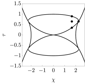
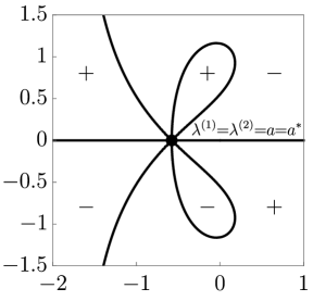
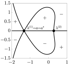
Figure 9. Signature charts of $\Re(\varphi(\lambda;\chi,\tau)-g(\lambda;\chi,\tau))$ for $\xi=i$ in the non-oscillatory region, along with the critical points $\lambda^{(1)}$ and $\lambda^{(2)}$ and the band endpoints $a$ and $a^{*}$. Top: $\chi=1.65$, $\tau\approx 0.8983$. Center left: Positions in the ($\chi$,$\tau$)-plane relative to the boundary curves. Center: $\chi=1.65$, $\tau=0.65$. Center right: $\chi=\frac{9}{4}$, $\tau=\frac{3\sqrt{3}}{8}$. Bottom: $\chi=1.65$, $\tau\approx 0.3488$.

Lemma 2.

In the non-oscillatory region, there is a domain $D_{\rm up}$ in the upper half-plane with the following properties:

• $D_{\rm up}$ contains $\xi$, is bounded by curves along which $\Re(\varphi(\lambda)-g(\lambda))=0$, and abuts the real axis along a single interval denoted by $(\lambda^{(1)},\lambda^{(2)})$.

• $\Re(\varphi(\lambda)-g(\lambda))>0$ for all $\lambda\in D_{\rm up}$.

• One arc of the boundary of $D_{\rm up}$ is the contour $\Sigma_{\rm up}:=\Sigma\cap\mathbb{C}^{+}$ from $\lambda^{(1)}$ to $a$, along which $\Re(\varphi(\lambda)-g(\lambda))>0$ for any $\lambda$ sufficiently close to either side of $\Sigma_{\rm up}$.

• The remaining boundary of $D_{\rm up}$ in the upper half-plane is a contour from $a$ to $\lambda^{(2)}$ (denoted $\Gamma_{\rm up}$) along which $\Re(\varphi(\lambda)-g(\lambda))<0$ for any $\lambda$ in the exterior of $\overline{D_{\rm up}}$ but sufficiently close to $D_{\rm up}$.

The domain $D_{\rm down}$ in the lower half-plane, defined as the reflection through the real axis of $D_{\rm up}$, has the following properties:

• $D_{\rm down}$ contains $\xi^{*}$, is bounded by curves along which $\Re(\varphi(\lambda)-g(\lambda))=0$, and abuts the real axis along the same interval as $D_{\rm up}$.

• $\Re(\varphi(\lambda)-g(\lambda))<0$ for all $\lambda\in D_{\rm down}$.

• One arc of the boundary of $D_{\rm down}$ is the contour $\Sigma_{\rm down}:=\Sigma\cap\mathbb{C}^{-}$ from $a^{*}$ to $\lambda^{(1)}$, along which $\Re(\varphi(\lambda)-g(\lambda))<0$ for any $\lambda$ sufficiently close to either side of $\Sigma_{\rm down}$.

• The remaining boundary of $D_{\rm down}$ in the lower half-plane is a contour from $\lambda^{(2)}$ to $a^{*}$ (denoted $\Gamma_{\rm down}$) along which $\Re(\varphi(\lambda)-g(\lambda))>0$ for any $\lambda$ in the exterior of $\overline{D_{\rm down}}$ but sufficiently close to $D_{\rm down}$.

Proof.

From (1.3) and (3.10) we see that

(3.17) $$\varphi^{\prime}(\lambda)-g^{\prime}(\lambda)=R(\lambda)\left(2i\tau-\frac{1}{R(\xi^{*})(\xi^{*}-\lambda)}+\frac{1}{R(\xi)(\xi-\lambda)}\right).$$

From here we see that $\phi^{\prime}(\lambda)-g^{\prime}(\lambda)$ has two square-root branch points at $a$ and $a^{*}$. Setting the term in parentheses equal to zero and rewriting as a quadratic expression in $\lambda$, we see $\phi^{\prime}(\lambda)-g^{\prime}(\lambda)$ also has two other zeros that we label as $\lambda^{(1)}$ and $\lambda^{(2)}$. The fact that $\lambda^{(1)}$ and $\lambda^{(2)}$ must be real, as well as the topological structure of the signature chart of $\Re(\varphi(\lambda)-g(\lambda))$, follows from analytic continuation from the boundary curve $\mathcal{L}_{\text{AN}}$ (at which $g(\lambda)\equiv 0$). See Figure 9. ∎

We now revisit the jump condition (3.2) and proceed with the determination of the constant $K$. Note that the endpoints $\lambda=a$ and $\lambda=a^{*}$ of $\Sigma$ have already been determined in the earlier construction. Recall that $g(\lambda)$ is analytic for $\lambda\in\mathbb{C}\setminus\Sigma$ with $g(\lambda)=\mathcal{O}(\lambda^{-1})$ as $\lambda\to\infty$. The fact that $\xi$ is contained in the region $D_{\mathrm{up}}$ and that $\Sigma_{\mathrm{up}}$ is a subset of the boundary of $D_{\mathrm{up}}$ ensures that $\Sigma\cap\Sigma_{\mathrm{c}}=\varnothing$. Thus, we may proceed as in [4] and express $g(\lambda)$ in the form $g(\lambda)=R(\lambda)k(\lambda)$, where $k(\lambda)$ is necessarily analytic for $\lambda\in\mathbb{C}\setminus\Sigma$ with continuous boundary values except at the endpoints $\lambda=a,a^{*}$ where $g(\lambda)$ is required to be bounded. Then, requiring $k(\lambda)=\mathcal{O}(\lambda^{-2})$ as $\lambda\to\infty$, (3.2) implies that

(3.18) $$k_{+}(\lambda)-k_{-}(\lambda)=\frac{2\varphi(\lambda)-2iK}{R_{+}(\lambda)},\quad\lambda\in\Sigma,$$

hence the Plemelj formula gives

(3.19) $$k(\lambda)=\frac{1}{i\pi}\int_{\Sigma}\frac{\varphi(s)-iK}{R_{+}(s)(s-\lambda)}\,ds.$$

Enforcing the condition $k(\lambda)=\mathcal{O}(\lambda^{-2})$ as $\lambda\to\infty$ in the representation (3.19) results in the condition

(3.20) $$\int_{\Sigma}\frac{\varphi(\lambda)-iK}{R_{+}(\lambda)}\,d\lambda=0.$$

First, recall that $R(\lambda)=\lambda+\mathcal{O}(1)$ as $\lambda\to\infty$. Thus, for an arbitrary clockwise-oriented loop $C$ surrounding the branch cut $\Sigma$ of $R(\lambda)$ we can obtain by a residue calculation at $\lambda=\infty$:

(3.21) $$\int_{\Sigma}\frac{d\lambda}{R_{+}(\lambda)}=\frac{1}{2}\oint_{C}\frac{d\lambda}{R(\lambda)}=-i\pi.$$

As the integral above is nonzero, the condition (3.20) successfully determines the constant $K$. The remaining integral

(3.22) $$\int_{\Sigma}\frac{\varphi(\lambda)}{R_{+}(\lambda)}\,d\lambda=\int_{\Sigma}\frac{i(\chi\lambda+\tau\lambda^{2})}{R_{+}(\lambda)}\,d\lambda+\int_{\Sigma}\frac{\log\left(\frac{\lambda-\xi^{*}}{\lambda-\xi}\right)}{R_{+}(\lambda)}\,d\lambda$$

in (3.20) can also be computed similarly. Using the expansion

(3.23) $$R(\lambda)^{-1}=\lambda^{-1}+\frac{1}{2}(a+a^{*})\lambda^{-2}+\frac{1}{4}\left((a+a^{*})^{2}+\frac{1}{2}(a-a^{*})^{2}\right)\lambda^{-3}+\mathcal{O}(\lambda^{-4}),\quad\lambda\to\infty,$$

we find that

(3.24) $$\int_{\Sigma}\frac{i(\chi\lambda+\tau\lambda^{2})}{R_{+}(\lambda)}\,d\lambda=\pi\left[\frac{1}{2}\chi(a+a^{*})+\frac{1}{4}\tau\left((a+a^{*})^{2}+\frac{1}{2}(a-a^{*})^{2}\right)\right].$$

Next, to evaluate the second integral on the right-hand side of (3.22) we again let $C$ be a clockwise-oriented loop surrounding the branch cut $\Sigma$ of $R(\lambda)$ but excluding the branch cut $\Sigma_{\mathrm{c}}$ of the logarithm in the integrand. Then, since the integrand is integrable at $\lambda=\infty$, letting $C^{\prime}$ be a counter-clockwise oriented contour that surrounds $\Sigma_{\mathrm{c}}$ but that excludes $\Sigma$ yields

(3.25) $$\int_{\Sigma}\frac{\log\left(\frac{\lambda-\xi^{*}}{\lambda-\xi}\right)}{R_{+}(\lambda)}\,d\lambda=\frac{1}{2}\oint_{C}\frac{\log\left(\frac{\lambda-\xi^{*}}{\lambda-\xi}\right)}{R(\lambda)}\,d\lambda=\frac{1}{2}\oint_{C^{\prime}}\frac{\log\left(\frac{\lambda-\xi^{*}}{\lambda-\xi}\right)}{R(\lambda)}\,d\lambda.$$

Now, recalling that $R(\lambda)$ is analytic on $\Sigma_{\mathrm{c}}$, we may collapse the contour $C^{\prime}$ to both sides of $\Sigma_{\mathrm{c}}$ and use the fact that the boundary values of the logarithm differ by $2\pi i$ on $\Sigma_{\mathrm{c}}$ to obtain

(3.26) $$\int_{\Sigma}\frac{\log\left(\frac{\lambda-\xi^{*}}{\lambda-\xi}\right)}{R_{+}(\lambda)}\,d\lambda=i\pi\int_{\Sigma_{\mathrm{c}}}\frac{1}{R(\lambda)}\,d\lambda.$$

Combining (3.24) and (3.26) gives

(3.27) $$\int_{\Sigma}\frac{\varphi(\lambda)}{R_{+}(\lambda)}\,d\lambda=\pi\left[\frac{1}{2}\chi(a+a^{*})+\frac{1}{4}\tau\left((a+a^{*})^{2}+\frac{1}{2}(a-a^{*})^{2}\right)\right]+i\pi\int_{\Sigma_{\mathrm{c}}}\frac{1}{R(\lambda)}\,d\lambda,$$

which, together with (3.22) results in

(3.28) $$K(\chi,\tau)=\left[\frac{1}{2}\chi(a+a^{*})+\frac{1}{4}\tau\left((a+a^{*})^{2}+\frac{1}{2}(a-a^{*})^{2}\right)\right]+i\int_{\Sigma_{\mathrm{c}}}\frac{1}{R(\lambda)}\,d\lambda,$$

which is real-valued.

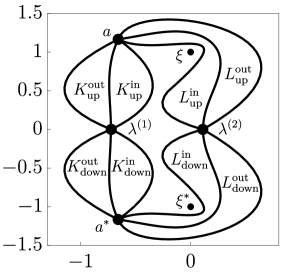
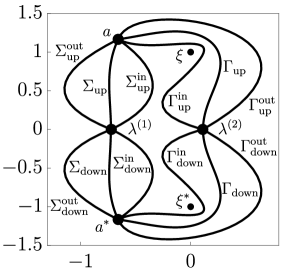
Figure 10. The domains (left) and contours (right) used in the definition of ${\bf Q}^{[n]}(\lambda)$ in the non-oscillatory region.

We are now ready to carry out the first Riemann-Hilbert transformation. Let the domain $D$ be the union of $D_{\rm up}$, $D_{\rm down}$, and the interval $(\lambda^{(1)},\lambda^{(2)})$. Note $D$ is bounded by $\Sigma_{\text{up}}\cup\Gamma_{\text{up}}\cup\Gamma_{\text{down}}\cup\Sigma_{\text{down}}$. Recall the function ${\bf N}^{[n]}(\lambda)$ satisfying Riemann-Hilbert Problem 2 and make the change of variables

(3.29) $${\bf O}^{[n]}(\lambda;\chi,\tau):=\begin{cases}{\bf N}^{[n]}(\lambda;\chi,\tau){\bf V}_{\bf N}^{[n]}(\lambda;\chi,\tau),&\lambda\in D_{0}\cap D^{\mathsf{c}},\\ {\bf N}^{[n]}(\lambda;\chi,\tau){\bf V}_{\bf N}^{[n]}(\lambda;\chi,\tau)^{-1},&\lambda\in D_{0}^{\mathsf{c}}\cap D,\\ {\bf N}^{[n]}(\lambda;\chi,\tau),&\text{otherwise}.\end{cases}$$

Now ${\bf O}^{[n]}(\lambda)$ satisfies the same Riemann-Hilbert problem as ${\bf N}^{[n]}(\lambda)$ with the jump contour $\partial D_{0}$ replaced by $\partial D$. Next, we introduce the $g$-function via

(3.30) $${\bf P}^{[n]}(\lambda;\chi,\tau):={\bf O}^{[n]}(\lambda;\chi,\tau)e^{-ng(\lambda;\chi,\tau)\sigma_{3}}.$$

The jump condition for ${\bf P}^{[n]}(\lambda)$ is now

(3.31) $${\bf P}_{+}^{[n]}(\lambda)={\bf P}_{-}^{[n]}(\lambda)e^{-n(\varphi(\lambda)-g_{-}(\lambda))\sigma_{3}}\mathcal{S}^{-1}e^{n(\varphi(\lambda)-g_{+}(\lambda))\sigma_{3}},\quad\lambda\in\partial D.$$

We define the following contours:

• $\Sigma_{\text{up}}^{\text{out}}$ runs from $\lambda^{(1)}$ to $a$ in the upper half-plane entirely in the region exterior to $D$ in which $\Re(\varphi(\lambda)-g(\lambda))>0$.

• $\Sigma_{\text{up}}^{\text{in}}$ runs from $\lambda^{(1)}$ to $a$ entirely in $D_{\rm up}$ (so $\Re(\varphi(\lambda)-g(\lambda))>0$), and can be deformed to $\Sigma_{\text{up}}$ without passing through $\xi$.

• $\Gamma_{\text{up}}^{\text{out}}$ runs from $a$ to $\lambda^{(2)}$ in the upper half-plane entirely in the region where $\Re(\varphi(\lambda)-g(\lambda))<0$.

• $\Gamma_{\text{up}}^{\text{in}}$ runs from $a$ to $\lambda^{(2)}$ entirely in $D_{\rm up}$ (so $\Re(\varphi(\lambda)-g(\lambda))>0$), and can be deformed to $\Gamma_{\text{up}}$ without passing through $\xi$.

• $\Sigma_{\text{down}}^{\text{out}}$ (oriented from $a^{*}$ to $\lambda^{(1)}$), $\Sigma_{\text{down}}^{\text{in}}$ (oriented from $a^{*}$ to $\lambda^{(1)}$), $\Gamma_{\text{down}}^{\text{out}}$ (oriented from $\lambda^{(2)}$ to $a^{*}$), and $\Gamma_{\text{down}}^{\text{in}}$ (oriented from $\lambda^{(2)}$ to $a^{*}$) are the reflections through the real axis of $\Sigma_{\text{up}}^{\text{out}}$, $\Sigma_{\text{up}}^{\text{in}}$, $\Gamma_{\text{up}}^{\text{out}}$, and $\Gamma_{\text{up}}^{\text{in}}$, respectively.

Define the following eight domains:

• $K_{\text{up}}^{\text{out}}$ (respectively, $K_{\text{up}}^{\text{in}}$) is the domain in the upper half-plane bounded by $\Sigma_{\text{up}}^{\text{out}}$ (respectively, $\Sigma_{\text{up}}^{\text{in}}$) and $\Sigma_{\text{up}}$.

• $L_{\text{up}}^{\text{out}}$ (respectively, $L_{\text{up}}^{\text{in}}$) is the domain in the upper half-plane bounded by $\Gamma_{\text{up}}^{\text{out}}$ (respectively, $\Gamma_{\text{up}}^{\text{in}}$) and $\Gamma_{\text{up}}$.

• $K_{\text{down}}^{\text{out}}$, $K_{\text{down}}^{\text{in}}$, $L_{\text{down}}^{\text{out}}$, and $L_{\text{down}}^{\text{in}}$ are the reflections through the real axis of $K_{\text{up}}^{\text{out}}$, $K_{\text{up}}^{\text{in}}$, $L_{\text{up}}^{\text{out}}$, and $L_{\text{up}}^{\text{in}}$, respectively.

See Figure 10. On $\Sigma$ we will use the following alternative factorizations of $\mathcal{S}^{-1}$:

(3.32) $$\begin{split}\mathcal{S}^{-1}&=\begin{bmatrix}1&-\frac{c_{1}^{*}}{c_{2}}\\ 0&1\end{bmatrix}\begin{bmatrix}0&\frac{|{\bf c}|}{c_{2}}\\ -\frac{c_{2}}{|{\bf c}|}&0\end{bmatrix}\begin{bmatrix}1&-\frac{c_{1}}{c_{2}}\\ 0&1\end{bmatrix}\quad\quad(\text{use for }\lambda\in\Sigma_{\text{up}}),\\ \mathcal{S}^{-1}&=\begin{bmatrix}1&0\\ \frac{c_{1}}{c_{2}^{*}}&1\end{bmatrix}\begin{bmatrix}0&\frac{c_{2}^{*}}{|{\bf c}|}\\ -\frac{|{\bf c}|}{c_{2}^{*}}&0\end{bmatrix}\begin{bmatrix}1&0\\ \frac{c_{1}^{*}}{c_{2}^{*}}&1\end{bmatrix}\quad\quad(\text{use for }\lambda\in\Sigma_{\text{down}}).\end{split}$$

We open lenses by defining

(3.33) $${\bf Q}^{[n]}(\lambda;\chi,\tau):=\begin{cases}{\bf P}^{[n]}(\lambda;\chi,\tau)\begin{bmatrix}1&-\frac{c_{1}^{*}}{c_{2}}e^{-2n(\varphi(\lambda;\chi,\tau)-g(\lambda;\chi,\tau))}\\ 0&1\end{bmatrix},&\lambda\in K_{\text{up}}^{\text{in}},\\ {\bf P}^{[n]}(\lambda;\chi,\tau)\begin{bmatrix}1&-\frac{c_{1}}{c_{2}}e^{-2n(\varphi(\lambda;\chi,\tau)-g(\lambda;\chi,\tau))}\\ 0&1\end{bmatrix}^{-1},&\lambda\in K_{\text{up}}^{\text{out}},\vspace{.025in}\\ {\bf P}^{[n]}(\lambda;\chi,\tau)\begin{bmatrix}1&0\\ \frac{c_{1}}{c_{2}^{*}}e^{2n(\varphi(\lambda;\chi,\tau)-g(\lambda;\chi,\tau))}&1\end{bmatrix},&\lambda\in K_{\text{down}}^{\text{in}},\\ {\bf P}^{[n]}(\lambda;\chi,\tau)\begin{bmatrix}1&0\\ \frac{c_{1}^{*}}{c_{2}^{*}}e^{2n(\varphi(\lambda;\chi,\tau)-g(\lambda;\chi,\tau))}&1\end{bmatrix}^{-1},&\lambda\in K_{\text{down}}^{\text{out}},\vspace{.025in}\\ {\bf P}^{[n]}(\lambda;\chi,\tau)\begin{bmatrix}1&\frac{c_{2}^{*}}{c_{1}}e^{-2n(\varphi(\lambda;\chi,\tau)-g(\lambda;\chi,\tau))}\\ 0&1\end{bmatrix},&\lambda\in L_{\text{up}}^{\text{in}},\\ {\bf P}^{[n]}(\lambda;\chi,\tau)\begin{bmatrix}1&0\\ -\frac{c_{2}}{c_{1}}e^{2n(\varphi(\lambda;\chi,\tau)-g(\lambda;\chi,\tau))}&1\end{bmatrix}^{-1},&\lambda\in L_{\text{up}}^{\text{out}},\vspace{.025in}\\ {\bf P}^{[n]}(\lambda;\chi,\tau)\begin{bmatrix}1&0\\ -\frac{c_{2}}{c_{1}^{*}}e^{2n(\varphi(\lambda;\chi,\tau)-g(\lambda;\chi,\tau))}&1\end{bmatrix},&\lambda\in L_{\text{down}}^{\text{in}},\\ {\bf P}^{[n]}(\lambda;\chi,\tau)\begin{bmatrix}1&\frac{c_{2}^{*}}{c_{1}^{*}}e^{-2n(\varphi(\lambda;\chi,\tau)-g(\lambda;\chi,\tau))}\\ 0&1\end{bmatrix}^{-1},&\lambda\in L_{\text{down}}^{\text{out}},\\ {\bf P}^{[n]}(\lambda;\chi,\tau),&\text{otherwise}.\end{cases}$$

Using (3.31), (3.32), and (2.2), we see that ${\bf Q}^{[n]}(\lambda)$ satisfies the jumps ${\bf Q}_{+}^{[n]}(\lambda)={\bf Q}_{-}^{[n]}(\lambda){\bf V}_{\bf Q}^{[n]}(\lambda)$, where the jumps on the various contours are given by

(3.34) $$\begin{aligned} &\Sigma_{\text{up}}:\,\,\begin{bmatrix}0&\frac{|{\bf c}|}{c_{2}}{e^{-2inK}}\\ -\frac{c_{2}}{|{\bf c}|}{e^{2inK}}&0\end{bmatrix},\quad&&\Sigma_{\text{down}}:\,\,\begin{bmatrix}0&\frac{c_{2}^{*}}{|{\bf c}|}{e^{-2inK}}\\ -\frac{|{\bf c}|}{c_{2}^{*}}{e^{2inK}}&0\end{bmatrix},\quad&&\Gamma_{\text{up}}:\,\,\begin{bmatrix}\frac{|{\bf c}|}{c_{1}}&0\\ 0&\frac{c_{1}}{|{\bf c}|}\end{bmatrix},\\ &\Gamma_{\text{down}}:\,\,\begin{bmatrix}\frac{c_{1}^{*}}{|{\bf c}|}&0\\ 0&\frac{|{\bf c}|}{c_{1}^{*}}\end{bmatrix},\quad&&\Sigma_{\text{up}}^{\text{in}}:\,\,\begin{bmatrix}1&-\frac{c_{1}^{*}}{c_{2}}e^{-2n(\varphi-g)}\\ 0&1\end{bmatrix},\quad&&\Sigma_{\text{up}}^{\text{out}}:\,\,\begin{bmatrix}1&-\frac{c_{1}}{c_{2}}e^{-2n(\varphi-g)}\\ 0&1\end{bmatrix},\\ &\Sigma_{\text{down}}^{\text{in}}:\begin{bmatrix}1&0\\ \frac{c_{1}}{c_{2}^{*}}e^{2n(\varphi-g)}&0\end{bmatrix},\quad&&\Sigma_{\text{down}}^{\text{out}}:\,\,\begin{bmatrix}1&0\\ \frac{c_{1}^{*}}{c_{2}^{*}}e^{2n(\varphi-g)}&0\end{bmatrix},\quad&&\Gamma_{\text{up}}^{\text{in}}:\,\,\begin{bmatrix}1&\frac{c_{2}^{*}}{c_{1}}e^{-2n(\varphi-g)}\\ 0&1\end{bmatrix},\\ \hskip 14.45377pt&\Gamma_{\text{up}}^{\text{out}}:\,\,\begin{bmatrix}1&0\\ -\frac{c_{2}}{c_{1}}e^{2n(\varphi-g)}&0\end{bmatrix},\quad&&\Gamma_{\text{down}}^{\text{in}}:\,\,\begin{bmatrix}1&0\\ -\frac{c_{2}}{c_{1}^{*}}e^{2n(\varphi-g)}&0\end{bmatrix},\quad&&\Gamma_{\text{down}}^{\text{out}}:\,\,\begin{bmatrix}1&\frac{c_{2}^{*}}{c_{1}^{*}}e^{-2n(\varphi-g)}\\ 0&1\end{bmatrix}.\hskip 72.26999pt\end{aligned}{3}$$

Lemma 2 shows that, except for the four constant jumps, all of the jumps decay exponentially to the identity for $\lambda$ bounded away from $a$, $a^{*}$, $\lambda^{(1)}$, and $\lambda^{(2)}$. We are thus ready to define the outer model Riemann-Hilbert problem.

Riemann-Hilbert Problem 4 (The outer model problem in the non-oscillatory region).

Fix a pole location $\xi\in\mathbb{C}^{+}$, a pair of nonzero complex numbers $(c_{1},c_{2})$, and a pair of real numbers $(\chi,\tau)$ in the non-oscillatory region. Determine the $2\times 2$ matrix ${\bf R}^{(\infty)}(\lambda;\chi,\tau)$ with the following properties:

• Analyticity: ${\bf R}^{(\infty)}(\lambda;\chi,\tau)$ is analytic for $\lambda\in\mathbb{C}$ except on $\Sigma_{\rm up}\cup\Sigma_{\rm down}\cup\Gamma_{\rm up}\cup\Gamma_{\rm down}$, where it achieves continuous boundary values on the interior of each arc.

• Jump condition: The boundary values taken by ${\bf R}^{(\infty)}(\lambda;\chi,\tau)$ are related by the jump conditions ${\bf R}^{(\infty)}_{+}(\lambda;\chi,\tau)={\bf R}^{(\infty)}_{-}(\lambda;\chi,\tau){\bf V}_{\bf R}^{(\infty)}(\lambda;\chi,\tau)$, where

  (3.35) $${\bf V}_{\bf R}^{(\infty)}(\lambda;\chi,\tau):=\begin{cases}\begin{bmatrix}0&\frac{|{\bf c}|}{c_{2}}{e^{-2inK}}\\ -\frac{c_{2}}{|{\bf c}|}{e^{2inK}}&0\end{bmatrix},&\lambda\in\Sigma_{\rm up},\vspace{.025in}\\ \begin{bmatrix}0&\frac{c_{2}^{*}}{|{\bf c}|}{e^{-2inK}}\\ -\frac{|{\bf c}|}{c_{2}^{*}}{e^{2inK}}&0\end{bmatrix},&\lambda\in\Sigma_{\rm down},\vspace{.025in}\\ \begin{bmatrix}\frac{|{\bf c}|}{c_{1}}&0\\ 0&\frac{c_{1}}{|{\bf c}|}\end{bmatrix},&\lambda\in\Gamma_{\rm up},\vspace{.025in}\\ \begin{bmatrix}\frac{c_{1}^{*}}{|{\bf c}|}&0\\ 0&\frac{|{\bf c}|}{c_{1}^{*}}\end{bmatrix},&\lambda\in\Gamma_{\rm down}.\end{cases}$$

• Normalization: As $\lambda\to\infty$, the matrix ${\bf R}^{(\infty)}(\lambda;\chi,\tau)$ satisfies the condition

  (3.36) $${\bf R}^{(\infty)}(\lambda;\chi,\tau)=\mathbb{I}+\mathcal{O}(\lambda^{-1})$$

  with the limit being uniform with respect to direction.

The first step in solving for ${\bf R}^{(\infty)}(\lambda)$ is to remove the dependence on $c_{1}$ and $c_{2}$. Define the function

(3.37) $$\begin{split}f(\lambda):=\frac{R(\lambda)}{2\pi i}&\left[\int_{\Sigma_{\rm up}}\frac{\log\left(\frac{c_{2}}{|{\bf c}|}\right)}{R_{+}(s)(s-\lambda)}ds+\int_{\Sigma_{\rm down}}\frac{\log\left(\frac{|{\bf c}|}{c_{2}^{*}}\right)}{R_{+}(s)(s-\lambda)}ds\right.\\ &\hskip 14.45377pt+\left.\int_{\Gamma_{\rm up}}\frac{\log\left(\frac{|{\bf c}|}{c_{1}}\right)}{R(s)(s-\lambda)}ds+\int_{\Gamma_{\rm down}}\frac{\log\left(\frac{c_{1}^{*}}{|{\bf c}|}\right)}{R(s)(s-\lambda)}ds\right].\end{split}$$

Then $f(\lambda)$ satisfies the jump conditions

(3.38) $$\begin{split}f_{+}(\lambda)+f_{-}(\lambda)&=-\log\left(\frac{|{\bf c}|}{c_{2}}\right),\quad\quad\lambda\in\Sigma_{\rm up},\\ f_{+}(\lambda)+f_{-}(\lambda)&=-\log\left(\frac{c_{2}^{*}}{|{\bf c}|}\right),\quad\quad\lambda\in\Sigma_{\rm down},\\ f_{+}(\lambda)-f_{-}(\lambda)&=-\log\left(\frac{c_{1}}{|{\bf c}|}\right),\quad\quad\lambda\in\Gamma_{\rm up},\\ f_{+}(\lambda)-f_{-}(\lambda)&=-\log\left(\frac{|{\bf c}|}{c_{1}^{*}}\right),\quad\quad\lambda\in\Gamma_{\rm down},\\ \end{split}$$

and the symmetry

(3.39) $$f(\lambda)=-(f(\lambda^{*}))^{*}.$$

We also have that $f(\lambda)$ is bounded as $\lambda\to\infty$, and

(3.40) $$\begin{split}f(\infty):=\lim_{\lambda\to\infty}f(\lambda)=-\frac{1}{2\pi i}&\left[\int_{\Sigma_{\rm up}}\frac{\log\left(\frac{c_{2}}{|{\bf c}|}\right)}{R_{+}(s)}ds+\int_{\Sigma_{\rm down}}\frac{\log\left(\frac{|{\bf c}|}{c_{2}^{*}}\right)}{R_{+}(s)}ds\right.\\ &\hskip 14.45377pt+\left.\int_{\Gamma_{\rm up}}\frac{\log\left(\frac{|{\bf c}|}{c_{1}}\right)}{R(s)}ds+\int_{\Gamma_{\rm down}}\frac{\log\left(\frac{c_{1}^{*}}{|{\bf c}|}\right)}{R(s)}ds\right].\end{split}$$

We note $f(\infty)$ is a purely imaginary number. Introduce

(3.41) $${\bf S}(\lambda):=e^{f(\infty)\sigma_{3}}{\bf R}^{(\infty)}(\lambda)e^{-f(\lambda)\sigma_{3}}.$$

Thus, we have ${\bf S}_{+}(\lambda)={\bf S}_{-}(\lambda){\bf V}_{\bf S}(\lambda)$, where

(3.42) $${\bf V}_{\bf S}(\lambda):=\begin{cases}\begin{bmatrix}0&\frac{|{\bf c}|}{c_{2}}e^{f_{+}(\lambda)+f_{-}(\lambda)}{e^{-2inK}}\\ -\frac{c_{2}}{|{\bf c}|}e^{-(f_{+}(\lambda)+f_{-}(\lambda))}{e^{2inK}}&0\end{bmatrix},&\lambda\in\Sigma_{\rm up},\vspace{.025in}\\ \begin{bmatrix}0&\frac{c_{2}^{*}}{|{\bf c}|}e^{f_{+}(\lambda)+f_{-}(\lambda)}{e^{-2inK}}\\ -\frac{|{\bf c}|}{c_{2}^{*}}e^{-(f_{+}(\lambda)+f_{-}(\lambda))}{e^{2inK}}&0\end{bmatrix},&\lambda\in\Sigma_{\rm down},\vspace{.025in}\\ \begin{bmatrix}\frac{|{\bf c}|}{c_{1}}e^{-(f_{+}(\lambda)-f_{-}(\lambda))}&0\\ 0&\frac{c_{1}}{|{\bf c}|}e^{f_{+}(\lambda)-f_{-}(\lambda)}\end{bmatrix},&\lambda\in\Gamma_{\rm up},\vspace{.025in}\\ \begin{bmatrix}\frac{c_{1}^{*}}{|{\bf c}|}e^{-(f_{+}(\lambda)-f_{-}(\lambda))}&0\\ 0&\frac{|{\bf c}|}{c_{1}^{*}}e^{f_{+}(\lambda)-f_{-}(\lambda)}\end{bmatrix},&\lambda\in\Gamma_{\rm down}.\end{cases}$$

From the conditions (3.38) for $f(\lambda)$ we see the jump simplifies to

(3.43) $${\bf S}_{+}(\lambda)={\bf S}_{-}(\lambda){e^{-inK\sigma_{3}}}\begin{bmatrix}0&1\\ -1&0\end{bmatrix}{e^{inK\sigma_{3}}},\quad\lambda\in\Sigma.$$

Along with the normalization condition ${\bf S}(\lambda)=\mathbb{I}+\mathcal{O}(\lambda^{-1})$, this specifies that ${\bf S}(\lambda)$ must be

(3.44) $${\bf S}(\lambda)={e^{-inK\sigma_{3}}}\begin{bmatrix}\displaystyle\frac{\gamma{{(\lambda)}}+\gamma{{(\lambda)}}^{-1}}{2}&\displaystyle\frac{-i\gamma{{(\lambda)}}+i\gamma{{(\lambda)}}^{-1}}{2}\\ \displaystyle\frac{i\gamma{{(\lambda)}}-i\gamma{{(\lambda)}}^{-1}}{2}&\displaystyle\frac{\gamma{{(\lambda)}}+\gamma{{(\lambda)}}^{-1}}{2}\end{bmatrix}{e^{inK\sigma_{3}}},$$

where

(3.45) $$\gamma(\lambda):=\left(\frac{\lambda-a}{\lambda-a^{*}}\right)^{1/4}$$

is cut on $\Sigma$ and has asymptotic behavior $\gamma(\lambda)=1+\mathcal{O}(\lambda^{-1})$ as $\lambda\to\infty$. Thus, we have

(3.46) $${\bf R}^{(\infty)}(\lambda)={e^{-inK\sigma_{3}}}\begin{bmatrix}\displaystyle\frac{\gamma{{(\lambda)}}+\gamma{{(\lambda)}}^{-1}}{2}e^{f(\lambda)-f(\infty)}&\displaystyle\frac{\gamma{{(\lambda)}}-\gamma{{(\lambda)}}^{-1}}{2i}e^{-f(\lambda)-f(\infty)}\\ \displaystyle-\frac{\gamma{{(\lambda)}}-\gamma{{(\lambda)}}^{-1}}{2i}e^{f(\lambda)+f(\infty)}&\displaystyle\frac{\gamma{{(\lambda)}}+\gamma{{(\lambda)}}^{-1}}{2}e^{-f(\lambda)+f(\infty)}\end{bmatrix}{e^{inK\sigma_{3}}}.$$

To complete the definition of the global model solution ${\bf R}(\lambda)$, we need to define local parametrices ${\bf R}^{(1)}(\lambda)$, ${\bf R}^{(2)}(\lambda)$, ${\bf R}^{(a)}(\lambda)$, and ${\bf R}^{(a^{*})}(\lambda)$ in small, fixed disks $\mathbb{D}^{(1)}$, $\mathbb{D}^{(2)}$, $\mathbb{D}^{(a)}$, and $\mathbb{D}^{(a^{*})}$ centered at $\lambda^{(1)}$, $\lambda^{(2)}$, $a$, and $a^{*}$, respectively. These local parametrices satisfy two conditions:

• ${\bf R}^{(\bullet)}(\lambda)$ satisfies the same jump conditions as ${\bf Q}^{[n]}(\lambda)$ for $\lambda\in\mathbb{D}^{(\bullet)}$, where $\bullet\in\{1,2,a,a^{*}\}$.

• ${\bf R}^{(\bullet)}(\lambda)=\begin{cases}{\bf R}^{(\infty)}(\lambda)(\mathbb{I}+\mathcal{O}(n^{-1/2})),&\lambda\in\partial\mathbb{D}^{(\bullet)},\text{ where }\bullet\in\{1,2\},\\ {\bf R}^{(\infty)}(\lambda)(\mathbb{I}+\mathcal{O}(n^{-1})),&\lambda\in\partial\mathbb{D}^{(\bullet)}\text{ where }\bullet\in\{a,a^{*}\}.\end{cases}$

While we will not need their explicit form, the parametrices ${\bf R}^{(1)}(\lambda)$ and ${\bf R}^{(2)}(\lambda)$ can be constructed explicitly using parabolic cylinder functions (see, for example, §2), while the parametrices ${\bf R}^{(1)}(\lambda)$ and ${\bf R}^{(2)}(\lambda)$ can be constructed explicitly using Airy functions (see, for example, [7]). Then the function

(3.47) $${\bf R}(\lambda):=\begin{cases}{\bf R}^{(1)}(\lambda),&\lambda\in\mathbb{D}^{(1)},\\ {\bf R}^{(2)}(\lambda),&\lambda\in\mathbb{D}^{(2)},\\ {\bf R}^{(a)}(\lambda),&\lambda\in\mathbb{D}^{(a)},\\ {\bf R}^{(a^{*})}(\lambda),&\lambda\in\mathbb{D}^{(a^{*})},\\ {\bf R}^{(\infty)}(\lambda),&\text{otherwise}\end{cases}$$

is a valid approximation to ${\bf Q}^{[n]}(\lambda)$ everywhere in the complex $\lambda$-plane as $n\to\infty$. In particular, we have

(3.48) $${\bf Q}^{[n]}(\lambda)=\left(\mathbb{I}+\mathcal{O}(n^{-1/2})\right){\bf R}(\lambda).$$

Working our way through the various transformations, we see that, for $|\lambda|$ sufficiently large,

(3.49) $$\begin{split}[{\bf M}^{[n]}&(\lambda;n\chi,n\tau)]_{12}=\left(\frac{\lambda-\xi^{*}}{\lambda-\xi}\right)^{n}[{\bf N}^{[n]}(\lambda;\chi,\tau)]_{12}=\left(\frac{\lambda-\xi^{*}}{\lambda-\xi}\right)^{n}[{\bf O}^{[n]}(\lambda;\chi,\tau)]_{12}\\ &=\left(\frac{\lambda-\xi^{*}}{\lambda-\xi}\right)^{n}e^{-ng(\lambda;\chi,\tau)}[{\bf P}^{[n]}(\lambda;\chi,\tau)]_{12}=\left(\frac{\lambda-\xi^{*}}{\lambda-\xi}\right)^{n}e^{-ng(\lambda;\chi,\tau)}[{\bf Q}^{[n]}(\lambda;\chi,\tau)]_{12}\\ &=\left(\frac{\lambda-\xi^{*}}{\lambda-\xi}\right)^{n}e^{-ng(\lambda;\chi,\tau)}\left([{\bf R}^{(\infty)}(\lambda;\chi,\tau)]_{12}+\mathcal{O}(n^{-1/2})\right)\\ &=\left(\frac{\lambda-\xi^{*}}{\lambda-\xi}\right)^{n}e^{-ng(\lambda;\chi,\tau)-f(\lambda;\chi,\tau)-f(\infty;\chi,\tau)}\left(\frac{\gamma(\lambda;\chi,\tau)-\gamma(\lambda;\chi,\tau)^{-1}}{2i}{e^{-2inK(\chi,\tau)}}+\mathcal{O}(n^{-1/2})\right).\end{split}$$

From

(3.50) $$\gamma(\lambda)-\gamma(\lambda)^{-1}=\frac{a^{*}-a}{2\lambda}+\mathcal{O}(\lambda^{-2}),$$

(3.51) $$\left(\frac{\lambda-\xi^{*}}{\lambda-\xi}\right)^{n}=1+\mathcal{O}(\lambda^{-1}),$$

and

(3.52) $$e^{-ng(\lambda)-f(\lambda)-f({\infty})}=e^{-2f(\infty)}+\mathcal{O}(\lambda^{-1}),$$

we see

(3.53) $$\lim_{\lambda\to\infty}\lambda[{\bf M}^{[n]}(\lambda;n\chi,n\tau)]_{12}=\frac{a^{*}(\chi,\tau)-a(\chi,\tau)}{4i}e^{-2f(\infty;\chi,\tau)}{e^{-2inK(\chi,\tau)}}+\mathcal{O}(n^{-1/2}).$$

Along with (1.21), this establishes Theorem 3.

4. The oscillatory region

Finally, we consider the oscillatory region. From the Riemann-Hilbert point of view, this region is distinguished by a two-band model problem. We begin by solving the following Riemann-Hilbert problem for $G(\lambda;\chi,\tau)$.

Riemann-Hilbert Problem 5 (The $G$-function in the oscillatory region).

Fix a pole location $\xi\in\mathbb{C}^{+}$, a pair of nonzero complex numbers $(c_{1},c_{2})$, and a pair of real numbers $(\chi,\tau)$ in the oscillatory region. Determine the unique contours $\Sigma_{\rm up}(\chi,\tau)$, $\Sigma_{\rm down}(\chi,\tau)$, and $\Gamma_{\rm mid}(\chi,\tau)$, the unique constants $\Omega(\chi,\tau)$ and $d(\chi,\tau)$, and the unique function $G(\lambda;\chi,\tau)$ satisfying the following conditions.

• Analyticity: $G(\lambda)$ is analytic for $\lambda\in\mathbb{C}$ except on $\Sigma_{\rm up}\cup\Sigma_{\rm down}\cup\Gamma_{\rm mid}$, where it achieves continuous boundary values. All three contours are simple and bounded. $\Sigma_{\rm down}$ is the reflection of $\Sigma_{\rm up}$ through the real axis. $\Gamma_{\rm mid}$ is symmetric across the real axis and connects $\Sigma_{\rm down}$ to $\Sigma_{\rm up}$.

• Jump condition: The boundary values taken by $G(\lambda)$ are related by the jump conditions

  (4.1) $$\begin{split}G_{+}(\lambda)+G_{-}(\lambda)&=2\varphi(\lambda)+\Omega,\quad\lambda\in\Sigma_{\rm up},\\ G_{+}(\lambda)+G_{-}(\lambda)&=2\varphi(\lambda)-\Omega^{*}=2\varphi(\lambda)+\Omega,\quad\lambda\in\Sigma_{\rm down},\\ G_{+}(\lambda)-G_{-}(\lambda)&=d,\quad\lambda\in\Gamma_{\rm mid}.\end{split}$$

  Here $\Omega$ and $d$ are purely imaginary constants. Furthermore,

  (4.2) $$\Re(\varphi(\lambda)-G_{+}(\lambda))=\Re(\varphi(\lambda)-G_{-}(\lambda))=0,\quad\lambda\in\Sigma_{\rm up}\cup\Sigma_{\rm down}\cup\Gamma_{\rm mid}.$$

• Normalization: As $\lambda\to\infty$, $G(\lambda)$ satisfies

  (4.3) $$G(\lambda)=\mathcal{O}\left(\lambda^{-1}\right)$$

  with the limit being uniform with respect to direction.

• Symmetry: $G(\lambda)$ satisfies the symmetry condition

  (4.4) $$G(\lambda)=-G(\lambda^{*})^{*}.\\$$

The symmetry condition immediately implies that $d$ is purely imaginary. However, the fact that $\Omega$ is purely imaginary is a condition on $\Sigma_{\text{up}}$ and $\Sigma_{\text{down}}$.

Assume that $\Sigma_{\text{up}}$ and $\Sigma_{\text{down}}$ are known. Suppose $\Sigma_{\text{up}}$ is oriented from $b\equiv b(\chi,\tau)$ to $a\equiv a(\chi,\tau)$ with $\Im(a)>\Im(b)$ and $\Sigma_{\text{down}}$ is oriented from $a^{*}$ to $b^{*}$. The band endpoints $a$ and $b$ are uniquely determined by the conditions

(4.5) $$G(\lambda)=\mathcal{O}(\lambda^{-1}),\quad\Re(\Omega)=0.$$

We now differentiate and solve for $G^{\prime}(\lambda)$. Observe that $G^{\prime}(\lambda)$ has jumps

(4.6) $$G^{\prime}_{+}(\lambda)+G^{\prime}_{-}(\lambda)=2i\chi+4i\lambda\tau+\frac{2}{\lambda-\xi^{*}}-\frac{2}{\lambda-\xi},\quad\quad\lambda\in\Sigma_{\text{up}}\cup\Sigma_{\text{down}}$$

and normalization

(4.7) $$G^{\prime}(\lambda)=\mathcal{O}(\lambda^{-2}),\quad\lambda\to\infty.$$

Define

(4.8) $$\mathfrak{R}(\lambda):=((\lambda-a)(\lambda-a^{*})(\lambda-b)(\lambda-b^{*}))^{1/2}$$

to be the function cut on $\Sigma_{\text{up}}\cup\Sigma_{\text{down}}$ with asymptotic behavior $\mathfrak{R}(\lambda)=\lambda^{2}+\mathcal{O}(\lambda)$ as $\lambda\to\infty.$ Note that if we define the symmetric functions

(4.9) $$\begin{split}\mathfrak{s}_{1}:=a+a^{*}+b+b^{*},\quad\mathfrak{s}_{2}:=aa^{*}+ab+ab^{*}+a^{*}b+a^{*}b^{*}+bb^{*},\\ \mathfrak{s}_{3}:=aa^{*}b+aa^{*}b^{*}+abb^{*}+a^{*}bb^{*},\quad\mathfrak{s}_{4}:=aa^{*}bb^{*},\hskip 39.74872pt\end{split}$$

then we can write

(4.10) $$\mathfrak{R}(\lambda)=(\lambda^{4}-\mathfrak{s}_{1}\lambda^{3}+\mathfrak{s}_{2}\lambda^{2}-\mathfrak{s}_{3}\lambda+\mathfrak{s}_{4})^{1/2}.$$

By the Plemelj formula, we have

(4.11) $$G^{\prime}(\lambda)=\frac{\mathfrak{R}(\lambda)}{2\pi i}\int_{\Sigma_{\text{up}}\cup\Sigma_{\text{down}}}\frac{2i\chi+4is\tau+\frac{2}{s-\xi^{*}}-\frac{2}{s-\xi}}{\mathfrak{R}_{+}(s)(s-\lambda)}ds.$$

Similar to the calculation for $g^{\prime}(\lambda)$ in §3, an explicit residue computation gives

(4.12) $$G^{\prime}(\lambda)=i\chi+2i\tau\lambda+\frac{1}{\lambda-\xi^{*}}-\frac{1}{\lambda-\xi}+\frac{\mathfrak{R}(\lambda)}{\mathfrak{R}(\xi^{*})(\xi^{*}-\lambda)}-\frac{\mathfrak{R}(\lambda)}{\mathfrak{R}(\xi)(\xi-\lambda)}.$$

We now present a computationally effective method of determining $a$ and $b$. Imposing the growth condition $G^{\prime}(\lambda)=\mathcal{O}(\lambda^{-2})$ leads to the following three conditions arising from requiring the terms proportional to $\lambda^{1}$, $\lambda^{0}$, and $\lambda^{-1}$ in the large-$\lambda$ expansion of (4.12) to be zero:

(4.13) $$\mathcal{O}(\lambda):\,2\tau+\frac{i}{\mathfrak{R}(\xi^{*})}-\frac{i}{\mathfrak{R}(\xi)}=0,$$

(4.14) $$\mathcal{O}(1):\,\chi+\tau\mathfrak{s}_{1}+\frac{i\xi^{*}}{\mathfrak{R}(\xi^{*})}-\frac{i\xi}{\mathfrak{R}(\xi)}=0,$$

(4.15) $$\mathcal{O}(\lambda^{-1}):\,\frac{\chi}{2}\mathfrak{s}_{1}+\tau\left(\frac{3}{4}\mathfrak{s}_{1}^{2}-\mathfrak{s}_{2}\right)+\frac{i(\xi^{*})^{2}}{\mathfrak{R}(\xi^{*})}-\frac{i\xi^{2}}{\mathfrak{R}(\xi)}=0.$$

These are three real conditions on the two complex unknowns $a$ and $b$ (the fourth condition will be $\Re(\Omega)=0$). Multiplying equation (4.13) by $\xi^{*}$ and plugging it into (4.14), we have

(4.16) $$\chi+\tau\mathfrak{s}_{1}-2\tau\xi^{*}=-i\frac{\xi^{*}-\xi}{\mathfrak{R}(\xi)}.$$

Next, multiplying equation (4.13) by $(\xi^{*})^{2}$ and plugging it into (4.15), we have

(4.17) $$\frac{\chi}{2}\mathfrak{s}_{1}+\tau\left(\frac{3}{4}\mathfrak{s}_{1}^{2}-\mathfrak{s}_{2}\right)-2\tau(\xi^{*})^{2}=-i\frac{(\xi^{*}-\xi)(\xi^{*}+\xi)}{\mathfrak{R}(\xi)}.$$

Then, multiplying equation (4.16) by $(\xi^{*}+\xi)$ and equating it with (4.17), we have

(4.18) $$\mathfrak{s}_{2}=\frac{3}{4}\mathfrak{s}_{1}^{2}+\left(\frac{1}{2}\frac{\chi}{\tau}-\xi^{*}-\xi\right)\mathfrak{s}_{1}+2\xi\xi^{*}-(\xi^{*}+\xi)\frac{\chi}{\tau},$$

which indicates that if $\mathfrak{s}_{1}$ is real then $\mathfrak{s}_{2}$ is real. Now use (4.18) to eliminate $\mathfrak{s}_{2}$ in (4.16) (here $\mathfrak{s}_{2}$ appears in $\mathfrak{R}(\xi)$). Take the real and imaginary parts to get two real equations on the three real variables $\mathfrak{s}_{1},\mathfrak{s}_{3}$, and $\mathfrak{s}_{4}$. These equations are both linear in $\mathfrak{s}_{3}$ and $\mathfrak{s}_{4}$, so $\mathfrak{s}_{3}$ and $\mathfrak{s}_{4}$ can be solved exactly in terms of $\mathfrak{s}_{1}$. Thus, given $\mathfrak{s}_{1}$, we can determine $\mathfrak{s}_{2}$, $\mathfrak{s}_{3}$, and $\mathfrak{s}_{4}$, from which the system (4.9) can be inverted to obtain $a$ and $b$. At this point we can define $G(\lambda)$ by

(4.19) $$G(\lambda):=\int_{\infty}^{\lambda}G^{\prime}(s)ds,$$

where the path of integration is chosen to avoid $\Sigma_{\text{up}}\cup\Sigma_{\text{down}}\cup\Gamma_{\text{mid}}$. Finally, we choose $\mathfrak{s}_{1}$ so that, once $a$ and $b$ and thus $G(\lambda)$ have been computed, $d:=G_{+}(\lambda)-G_{-}(\lambda)$ is purely imaginary (here $d$ is independent of $\lambda$ as long as $\lambda\in\Gamma_{\text{mid}}$).

The final step in the definition of $G(\lambda)$ is the choice of cuts. Similar to the non-oscillatory case, we note from (4.11) that shifting $\Sigma_{\text{up}}$ or $\Sigma_{\text{down}}$ only changes $G(\lambda)$ by at most a sign, and so has no effect on the placement of the contours along which $\Re(\varphi(\lambda)-G(\lambda))=0$. Therefore, we redefine $\Sigma_{\text{up}}$ to be the simple contour from $b$ to $a$ along which $\Re(\varphi(\lambda)-G(\lambda))=0$ and $\Re(\varphi(\lambda)-G(\lambda))$ is positive to either side. The symmetry condition (4.4) then forces $\Sigma_{\text{down}}$ to be the reflection of $\Sigma_{\text{up}}$ through the real axis. We also choose $\Gamma_{\text{mid}}$ (whose main role is to restrict the integration path in (4.19)) to be the contour from $b^{*}$ to $b$ along which $\Re(\varphi(\lambda)-G(\lambda))=0$. The fact that such contours exist along which $\Re(\varphi(\lambda)-G(\lambda))=0$ is proven next in Lemma 3.

Lemma 3.

In the oscillatory region, there is a domain $D_{\rm up}$ in the upper half-plane with the following properties:

• $D_{\rm up}$ contains $\xi$ and is bounded by a simple Jordan curve along which $\Re(\varphi(\lambda)-G(\lambda))=0$. This curve contains the points $a$ and $b$.

• $\Re(\varphi(\lambda)-G(\lambda))>0$ for all $\lambda\in D_{\rm up}$.

• One arc of the boundary of $D_{\rm up}$ is the contour $\Sigma_{\rm up}$ from $b$ to $a$, along which $\Re(\varphi(\lambda)-G(\lambda))>0$ for any $\lambda$ sufficiently close to either side of $\Sigma_{\rm up}$.

• The remaining boundary of $D_{\rm up}$ is a contour from $a$ to $b$ (denoted $\Gamma_{\rm up}$) along which $\Re(\varphi(\lambda)-G(\lambda))<0$ for any $\lambda$ in the exterior of $\overline{D_{\rm up}}$ but sufficiently close to $D_{\rm up}$.

The domain $D_{\rm down}$ in the lower half-plane, defined as the reflection of $D_{\rm up}$ through the real axis, has the following properties:

• $D_{\rm down}$ contains $\xi^{*}$ and is bounded by a simple Jordan curve along which $\Re(\varphi(\lambda)-G(\lambda))=0$.

• $\Re(\varphi(\lambda)-G(\lambda))<0$ for all $\lambda\in D_{\rm down}$.

• One arc of the boundary of $D_{\rm down}$ is a contour (denoted $\Sigma_{\rm down}$) from $a^{*}$ to $b^{*}$, along which $\Re(\varphi(\lambda)-G(\lambda))<0$ for any $\lambda$ sufficiently close to either side of $\Sigma_{\rm down}$.

• The remaining boundary of $D_{\rm down}$ is a contour from $b^{*}$ to $a^{*}$ (denoted $\Gamma_{\rm down}$) along which $\Re(\varphi(\lambda)-G(\lambda))>0$ for any $\lambda$ in the exterior of $\overline{D_{\rm down}}$ but sufficiently close to $D_{\rm down}$.

Proof.

The proof is similar to that of Lemma 2. From (1.3) and (4.12), we see

(4.20) $$\varphi^{\prime}(\lambda)-G^{\prime}(\lambda)=\mathfrak{R}(\lambda)\left(\frac{1}{\mathfrak{R}(\xi)(\xi-\lambda)}-\frac{1}{\mathfrak{R}(\xi^{*})(\xi^{*}-\lambda)}\right).$$

From the first factor $\mathfrak{R}(\lambda)$, we see $\varphi^{\prime}(\lambda)-G^{\prime}(\lambda)$ has four square-root branch points and the same branch cut as $\mathfrak{R}(\lambda)$. From the second factor we can clear denominators and see that $\varphi(\lambda)-G(\lambda)$ has exactly one critical point. By symmetry this critical point must lie on the real axis, and thus on a curve on which $\varphi(\lambda)-G(\lambda)=0$. The topology of the level curves and the structure of the signature chart of $\Re(\varphi(\lambda)-G(\lambda))$ is deduced from analytic continuation from either $\mathcal{L}_{\text{NO}}$ (the shared boundary with the non-oscillatory region) or from $\mathcal{L}_{\text{EO}}$ (the shared boundary with the exponential-decay region). ∎

The signature chart of $\Re(\varphi(\lambda)-G(\lambda))$ is illustrated in Figure 11. We now begin our transformations of Riemann-Hilbert Problem 2. Define

(4.21) $${\bf O}^{[n]}(\lambda;\chi,\tau):=\begin{cases}{\bf N}^{[n]}(\lambda;\chi,\tau){\bf V}_{\bf N}^{[n]}(\lambda;\chi,\tau),&\lambda\in D_{0}\cap(D_{\rm up}\cup D_{\rm down})^{\mathsf{c}},\\ {\bf N}^{[n]}(\lambda;\chi,\tau){\bf V}_{\bf N}^{[n]}(\lambda;\chi,\tau)^{-1},&\lambda\in D_{0}^{\mathsf{c}}\cap(D_{\rm up}\cup D_{\rm down}),\\ {\bf N}^{[n]}(\lambda;\chi,\tau),&\text{otherwise}.\end{cases}$$

The jump for ${\bf O}^{[n]}(\lambda)$ lies on $\Sigma_{\text{up}}\cup\Sigma_{\text{down}}\cup\Gamma_{\text{up}}\cup\Gamma_{\text{down}}$. Next, define

(4.22) $${\bf P}^{[n]}(\lambda;\chi,\tau):={\bf O}^{[n]}(\lambda;\chi,\tau)e^{-nG(\lambda)\sigma_{3}}.$$

The matrix ${\bf P}^{[n]}(\lambda)$ has an additional jump on $\Gamma_{\text{mid}}$, namely

(4.23) $${\bf P}_{+}^{[n]}(\lambda)={\bf P}_{-}^{[n]}(\lambda)\begin{bmatrix}e^{-n(G_{+}(\lambda)-G_{-}(\lambda))}&0\\ 0&e^{n(G_{+}(\lambda)-G_{-}(\lambda))}\end{bmatrix}={\bf P}_{-}^{[n]}(\lambda)\begin{bmatrix}e^{-nd}&0\\ 0&e^{nd}\end{bmatrix},\quad\lambda\in\Gamma_{\text{mid}}.$$

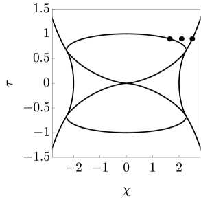
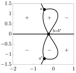
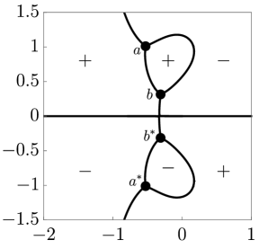
Figure 11. Signature charts of $\Re(\varphi(\lambda;\chi,\tau)-G(\lambda;\chi,\tau))$ for $\xi=i$ in the oscillatory region, along with the band endpoints $a$, $a^{*}$, $b$, and $b^{*}$. Top: Positions in the ($\chi$,$\tau$)-plane relative to the boundary curves. Bottom right: $\chi=1.65$, $\tau\approx 0.8983$. Bottom middle: $\chi=2.1$, $\tau=0.9$. Bottom right: $\chi\approx 2.502$, $\tau=0.9$.

Analogously to the non-oscillatory region, we define the contours

• $\Sigma_{\text{up}}^{\text{out}}$ runs from $b$ to $a$ in the upper half-plane entirely in the region exterior to $D_{\rm up}$ in which $\Re(\varphi(\lambda)-G(\lambda))>0$.

• $\Sigma_{\text{up}}^{\text{in}}$ runs from $b$ to $a$ entirely in $D_{\rm up}$ (so $\Re(\varphi(\lambda)-G(\lambda))>0$), and can be deformed to $\Sigma_{\text{up}}$ without passing through $\xi$.

• $\Gamma_{\text{up}}^{\text{out}}$ runs from $a$ to $b$ in the upper half-plane entirely in the region where $\Re(\varphi(\lambda)-G(\lambda))<0$.

• $\Gamma_{\text{up}}^{\text{in}}$ runs from $a$ to $b$ entirely in $D_{\rm up}$ (so $\Re(\varphi(\lambda)-G(\lambda))>0$), and can be deformed to $\Gamma_{\text{up}}$ without passing through $\xi$.

• $\Sigma_{\text{down}}^{\text{out}}$ (oriented from $a^{*}$ to $b^{*}$), $\Sigma_{\text{down}}^{\text{in}}$ (oriented from $a^{*}$ to $b^{*}$), $\Gamma_{\text{down}}^{\text{out}}$ (oriented from $b^{*}$ to $a^{*}$), and $\Gamma_{\text{down}}^{\text{in}}$ (oriented from $b^{*}$ to $a^{*}$) are the reflections through the real axis of $\Sigma_{\text{up}}^{\text{out}}$, $\Sigma_{\text{up}}^{\text{in}}$, $\Gamma_{\text{up}}^{\text{out}}$, and $\Gamma_{\text{up}}^{\text{in}}$, respectively.

Also define the domains

• $K_{\text{up}}^{\text{out}}$ (respectively, $K_{\text{up}}^{\text{in}}$) is the domain in the upper half-plane bounded by $\Sigma_{\text{up}}^{\text{out}}$ (respectively, $\Sigma_{\text{up}}^{\text{in}}$) and $\Sigma_{\text{up}}$.

• $L_{\text{up}}^{\text{out}}$ (respectively, $L_{\text{up}}^{\text{in}}$) is the domain in the upper half-plane bounded by $\Gamma_{\text{up}}^{\text{out}}$ (respectively, $\Gamma_{\text{up}}^{\text{in}}$) and $\Gamma_{\text{up}}$.

• $K_{\text{down}}^{\text{out}}$, $K_{\text{down}}^{\text{in}}$, $L_{\text{down}}^{\text{out}}$, and $L_{\text{down}}^{\text{in}}$ are the reflections through the real axis of $K_{\text{up}}^{\text{out}}$, $K_{\text{up}}^{\text{in}}$, $L_{\text{up}}^{\text{out}}$, and $L_{\text{up}}^{\text{in}}$, respectively.

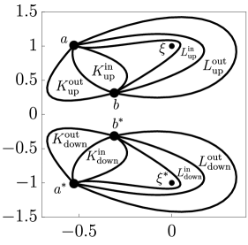
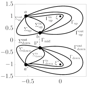
Figure 12. The domains (left) and contours (right) used in the definition of ${\bf Q}^{[n]}(\lambda)$ in the oscillatory region. The contour $\Gamma_{\text{mid}}$ is denoted by a dotted line.

See Figure 12. Then we define ${\bf Q}^{[n]}(\lambda)$ by opening lenses as in (3.33) (except with $g(\lambda)$ replaced by $G(\lambda)$). The jump matrices for ${\bf Q}^{[n]}(\lambda)$ are as follows:

(4.24) $$\begin{split}\Sigma_{\text{up}}:\,\,\begin{bmatrix}0&\frac{|{\bf c}|}{c_{2}}e^{n\Omega}\\ -\frac{c_{2}}{|{\bf c}|}e^{-n\Omega}&0\end{bmatrix},\quad\Sigma_{\text{down}}:\,\,\begin{bmatrix}0&\frac{c_{2}^{*}}{|{\bf c}|}e^{n\Omega}\\ -\frac{|{\bf c}|}{c_{2}^{*}}e^{-n\Omega}&0\end{bmatrix},\hskip 67.21056pt\\ \Gamma_{\text{up}}:\,\,\begin{bmatrix}\frac{|{\bf c}|}{c_{1}}&0\\ 0&\frac{c_{1}}{|{\bf c}|}\end{bmatrix},\quad\Gamma_{\text{down}}:\,\,\begin{bmatrix}\frac{c_{1}^{*}}{|{\bf c}|}&0\\ 0&\frac{|{\bf c}|}{c_{1}^{*}}\end{bmatrix},\quad\Gamma_{\text{mid}}:\,\,\begin{bmatrix}e^{-nd}&0\\ 0&e^{nd}\end{bmatrix},\hskip 61.42993pt\\ \Sigma_{\text{up}}^{\text{in}}:\,\,\begin{bmatrix}1&-\frac{c_{1}^{*}}{c_{2}}e^{-2n(\varphi-G)}\\ 0&1\end{bmatrix},\quad\Sigma_{\text{up}}^{\text{out}}:\,\,\begin{bmatrix}1&-\frac{c_{1}}{c_{2}}e^{-2n(\varphi-G)}\\ 0&1\end{bmatrix},\quad\Sigma_{\text{down}}^{\text{in}}:\,\,\begin{bmatrix}1&0\\ \frac{c_{1}}{c_{2}^{*}}e^{2n(\varphi-G)}&0\end{bmatrix},\\ \Sigma_{\text{down}}^{\text{out}}:\,\,\begin{bmatrix}1&0\\ \frac{c_{1}^{*}}{c_{2}^{*}}e^{2n(\varphi-G)}&0\end{bmatrix},\quad\Gamma_{\text{up}}^{\text{in}}:\,\,\begin{bmatrix}1&\frac{c_{2}^{*}}{c_{1}}e^{-2n(\varphi-G)}\\ 0&1\end{bmatrix},\quad\Gamma_{\text{up}}^{\text{out}}:\,\,\begin{bmatrix}1&0\\ -\frac{c_{2}}{c_{1}}e^{2n(\varphi-G)}&0\end{bmatrix},\hskip 14.45377pt\\ \Gamma_{\text{down}}^{\text{in}}:\,\,\begin{bmatrix}1&0\\ -\frac{c_{2}}{c_{1}^{*}}e^{2n(\varphi-G)}&0\end{bmatrix},\quad\Gamma_{\text{down}}^{\text{out}}:\,\,\begin{bmatrix}1&\frac{c_{2}^{*}}{c_{1}^{*}}e^{-2n(\varphi-G)}\\ 0&1\end{bmatrix}.\hskip 72.26999pt\end{split}$$

Lemma 3 shows that all of the non-constant jump matrices decay exponentially fast to the identity matrix outside of small fixed neighborhoods $\mathbb{D}^{(a)}$, $\mathbb{D}^{(b)}$, $\mathbb{D}^{(a^{*})}$, and $\mathbb{D}^{(b^{*})}$ of $a$, $b$, $a^{*}$, and $b^{*}$, respectively. We therefore arrive at the outer model problem.

Riemann-Hilbert Problem 6 (The outer model problem in the oscillatory region).

Fix a pole location $\xi\in\mathbb{C}^{+}$, a pair of nonzero complex numbers $(c_{1},c_{2})$, and a pair of real numbers $(\chi,\tau)$ in the oscillatory region. Determine the $2\times 2$ matrix ${\bf R}^{(\infty)}(\lambda;\chi,\tau)$ with the following properties:

• Analyticity: ${\bf R}^{(\infty)}(\lambda;\chi,\tau)$ is analytic for $\lambda\in\mathbb{C}$ except on $\Sigma_{\rm up}\cup\Sigma_{\rm down}\cup\Gamma_{\rm up}\cup\Gamma_{\rm down}\cup\Gamma_{\rm mid}$, where it achieves continuous boundary values on the interior of each arc.

• Jump condition: The boundary values taken by ${\bf R}^{(\infty)}(\lambda;\chi,\tau)$ are related by the jump conditions ${\bf R}^{(\infty)}_{+}(\lambda;\chi,\tau)={\bf R}^{(\infty)}_{-}(\lambda;\chi,\tau){\bf V}_{\bf R}^{(\infty)}(\lambda;\chi,\tau)$, where

  (4.25) $${\bf V}_{\bf R}^{(\infty)}(\lambda;\chi,\tau):=\begin{cases}\begin{bmatrix}0&\frac{|{\bf c}|}{c_{2}}e^{n\Omega}\\ -\frac{c_{2}}{|{\bf c}|}e^{-n\Omega}&0\end{bmatrix},&\lambda\in\Sigma_{\rm up},\vspace{.025in}\\ \begin{bmatrix}0&\frac{c_{2}^{*}}{|{\bf c}|}e^{n\Omega}\\ -\frac{|{\bf c}|}{c_{2}^{*}}e^{-n\Omega}&0\end{bmatrix},&\lambda\in\Sigma_{\rm down},\vspace{.025in}\\ \begin{bmatrix}\frac{|{\bf c}|}{c_{1}}&0\\ 0&\frac{c_{1}}{|{\bf c}|}\end{bmatrix},&\lambda\in\Gamma_{\rm up},\vspace{.025in}\\ \begin{bmatrix}\frac{c_{1}^{*}}{|{\bf c}|}&0\\ 0&\frac{|{\bf c}|}{c_{1}^{*}}\end{bmatrix},&\lambda\in\Gamma_{\rm down},\vspace{.025in}\\ \begin{bmatrix}e^{-nd}&0\\ 0&e^{nd}\end{bmatrix},&\lambda\in\Gamma_{\rm mid}.\end{cases}$$

• Normalization: As $\lambda\to\infty$, the matrix ${\bf R}^{(\infty)}(\lambda;\chi,\tau)$ satisfies the condition

  (4.26) $${\bf R}^{(\infty)}(\lambda;\chi,\tau)=\mathbb{I}+\mathcal{O}(\lambda^{-1})$$

  with the limit being uniform with respect to direction.

To remove the dependence on $c_{1}$, $c_{2}$, $\Omega$, and $d$, we define

(4.27) $$\begin{split}F(\lambda):=\frac{\mathfrak{R}(\lambda)}{2\pi i}\left(\int_{\Sigma_{\text{up}}}\frac{-n\Omega-\log\left(\frac{|{\bf c}|}{c_{2}}\right)}{\mathfrak{R}_{+}(s)(s-\lambda)}ds+\int_{\Sigma_{\text{down}}}\frac{-n\Omega-\log\left(\frac{c_{2}^{*}}{|{\bf c}|}\right)}{\mathfrak{R}_{+}(s)(s-\lambda)}ds\right.\hskip 86.72377pt\\ \left.+\int_{\Gamma_{\rm up}}\frac{\log\left(\frac{|{\bf c}|}{c_{1}}\right)}{\mathfrak{R}(s)(s-\lambda)}ds+\int_{\Gamma_{\rm down}}\frac{\log\left(\frac{c_{1}^{*}}{|{\bf c}|}\right)}{\mathfrak{R}(s)(s-\lambda)}ds+\int_{\Gamma_{\text{mid}}}\frac{-nd}{\mathfrak{R}(s)(s-\lambda)}ds\right).\end{split}$$

Here $F(\lambda)$ satisfies the jump conditions

(4.28) $$\begin{split}F_{+}+F_{-}&=-n\Omega-\log\left(\frac{|{\bf c}|}{c_{2}}\right),\quad\lambda\in\Sigma_{\text{up}},\\ F_{+}+F_{-}&=-n\Omega-\log\left(\frac{c_{2}^{*}}{|{\bf c}|}\right),\quad\lambda\in\Sigma_{\text{down}},\\ F_{+}-F_{-}&=\log\left(\frac{|{\bf c}|}{c_{1}}\right),\quad\lambda\in\Gamma_{\rm up},\\ F_{+}-F_{-}&=\log\left(\frac{c_{1}^{*}}{|{\bf c}|}\right),\quad\lambda\in\Gamma_{\rm down},\\ F_{+}-F_{-}&=-nd,\quad\lambda\in\Gamma_{\text{mid}}\end{split}$$

and the symmetry

(4.29) $$F(\lambda)=-(F(\lambda^{*}))^{*}.$$

As $\lambda\to\infty$ we have

(4.30) $$F(\lambda)=F_{1}\lambda+F_{0}+\mathcal{O}(\lambda^{-1}),$$

where

(4.31) $$\begin{split}F_{1}:=\frac{-1}{2\pi i}\left(\int_{\Sigma_{\text{up}}}\frac{-n\Omega-\log\left(\frac{|{\bf c}|}{c_{2}}\right)}{\mathfrak{R}_{+}(s)}ds+\int_{\Sigma_{\text{down}}}\frac{-n\Omega-\log\left(\frac{c_{2}^{*}}{|{\bf c}|}\right)}{\mathfrak{R}_{+}(s)}ds\right.\hskip 57.81621pt\\ \left.+\int_{\Gamma_{\rm up}}\frac{\log\left(\frac{|{\bf c}|}{c_{1}}\right)}{\mathfrak{R}(s)}ds+\int_{\Gamma_{\rm down}}\frac{\log\left(\frac{c_{1}^{*}}{|{\bf c}|}\right)}{\mathfrak{R}(s)}ds+\int_{\Gamma_{\text{mid}}}\frac{-nd}{\mathfrak{R}(s)(s-\lambda)}ds\right)\end{split}$$

and

(4.32) $$\begin{split}F_{0}:=-\frac{\mathfrak{s}_{1}}{2}F_{1}-\frac{1}{2\pi i}\left(\int_{\Sigma_{\text{up}}}\frac{-n\Omega-\log\left(\frac{|{\bf c}|}{c_{2}}\right)}{\mathfrak{R}_{+}(s)}sds+\int_{\Sigma_{\text{down}}}\frac{-n\Omega-\log\left(\frac{c_{2}^{*}}{|{\bf c}|}\right)}{\mathfrak{R}_{+}(s)}sds\right.\hskip 43.36243pt\\ \left.+\int_{\Gamma_{\rm up}}\frac{\log\left(\frac{|{\bf c}|}{c_{1}}\right)}{\mathfrak{R}(s)}sds+\int_{\Gamma_{\rm down}}\frac{\log\left(\frac{c_{1}^{*}}{|{\bf c}|}\right)}{\mathfrak{R}(s)}sds+\int_{\Gamma_{\text{mid}}}\frac{-nd}{\mathfrak{R}(s)(s-\lambda)}sds\right).\end{split}$$

Define

(4.33) $${\bf S}(\lambda):=e^{F_{0}\sigma_{3}}{\bf R}^{(\infty)}(\lambda)e^{-F(\lambda)\sigma_{3}}.$$

Then ${\bf S}(\lambda)$ is analytic for $\lambda\notin\Sigma_{\text{up}}\cup\Sigma_{\text{down}}$, has jumps

(4.34) $${\bf S}_{+}(\lambda)={\bf S}_{-}(\lambda)\begin{bmatrix}0&1\\ -1&0\end{bmatrix},\quad\lambda\in\Sigma_{\text{up}}\cup\Sigma_{\text{down}},$$

and has large-$\lambda$ behavior

(4.35) $${\bf S}(\lambda)e^{F_{1}\lambda\sigma_{3}}=\mathbb{I}+\mathcal{O}(\lambda^{-1}),\quad\lambda\to\infty.$$

We now build ${\bf S}(\lambda)$ explicitly out of Riemann-theta functions. See [5, 6], for example, for similar constructions. The function $\mathfrak{R}(\lambda)$ defines a genus-one Riemann surface constructed from two copies of the complex plane cut on $\Sigma_{\text{up}}$ and $\Sigma_{\text{down}}$. We introduce a basis of homology cycles $\{\mathfrak{a},\mathfrak{b}\}$ as shown in Figure 13. Here integration on the second sheet is accomplished by replacing $\mathfrak{R}(\lambda)$ by $-\mathfrak{R}(\lambda)$.

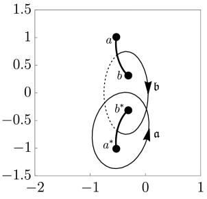
Figure 13. The homology cycles $\mathfrak{a}$ and $\mathfrak{b}$ in relation to the branch cuts of $\mathfrak{R}(\lambda)$. Thin solid lines lie on the first sheet while the dotted line lies on the second sheet.

Define the Abel map as

(4.36) $$A(\lambda):=\frac{2\pi i}{\oint_{\mathfrak{a}}\frac{ds}{\mathfrak{R}(s)}}\int_{a^{*}}^{\lambda}\frac{ds}{\mathfrak{R}(s)}.$$

We think of the integration as being on the Riemann surface (i.e. if the integration path passes through a branch cut then $\mathfrak{R}(\lambda)$ flips to $-\mathfrak{R}(\lambda)$). The Abel map depends on the integration contour and changes value if an extra $\mathfrak{a}$ cycle or $\mathfrak{b}$ cycle is added. In particular, adding an extra $\mathfrak{a}$ cycle to the integration contour adds $2\pi i$ to the Abel map, while an extra $\mathfrak{b}$ cycle adds the quantity

(4.37) $$B:=\frac{2\pi i}{\oint_{\mathfrak{a}}\frac{ds}{\mathfrak{R}(s)}}\oint_{\mathfrak{b}}\frac{ds}{\mathfrak{R}(s)}.$$

We define the lattice

(4.38) $$\Lambda:=2\pi ij+Bk,\quad j,k\in\mathbb{Z}.$$

Then the Abel map is well-defined modulo $\Lambda$. We compute

(4.39) $$\begin{split}A_{+}(\lambda)+A_{-}(\lambda)&=-B\text{ mod }\Lambda,\quad\lambda\in\Sigma_{\text{up}},\\ A_{+}(\lambda)-A_{-}(\lambda)&=-2\pi i\text{ mod }\Lambda,\quad\lambda\in\Gamma_{\text{mid}},\\ A_{+}(\lambda)+A_{-}(\lambda)&=0\text{ mod }\Lambda,\quad\lambda\in\Sigma_{\text{down}}.\end{split}$$

We now define two differentials $\omega$ and $\Delta$. Let

(4.40) $$\omega:=\frac{2\pi i}{\oint_{\mathfrak{a}}\frac{ds}{\mathfrak{R}(s)}}\frac{ds}{\mathfrak{R}(s)}$$

be the holomorphic differential normalized so $\oint_{\mathfrak{a}}\omega=2\pi i$. We also define

(4.41) $$\Delta_{0}:=\frac{s^{2}-\frac{1}{2}\mathfrak{s}_{1}s}{\mathfrak{R}(s)}ds,\quad\Delta=\Delta_{0}-\left(\frac{1}{2\pi i}\oint_{\mathfrak{a}}\Delta_{0}\right)\omega$$

so that $\oint_{\mathfrak{a}}\Delta=0$. Here $\Delta_{0}$ is chosen to ensure that

(4.42) $$J:=\lim_{\lambda\to\infty}\left(\lambda-\int_{a^{*}}^{\lambda}\Delta\right)$$

exists. We also set

(4.43) $$U:=\oint_{\mathfrak{b}}\Delta.$$

Now $\int_{a^{*}}^{\lambda}\Delta$ satisfies the jump conditions

(4.44) $$\begin{split}\int_{a^{*}}^{\lambda_{+}}\Delta&=-U-\int_{a^{*}}^{\lambda_{-}}\Delta,\quad\lambda\in\Sigma_{\text{up}},\\ \int_{a^{*}}^{\lambda_{+}}\Delta&=-\int_{a^{*}}^{\lambda_{-}}\Delta,\quad\lambda\in\Sigma_{\text{down}}\end{split}$$

(here we restrict the integration path to be on the first sheet). The Riemann-theta function defined by (1.16) has the properties [13]

(4.45) $$\Theta(-\lambda)=\Theta(\lambda),\quad\Theta(\lambda+2\pi i)=\Theta(\lambda),\quad\Theta(\lambda+B)=e^{-\frac{1}{2}B}e^{-\lambda}\Theta(\lambda).$$

Also $\Theta(\lambda)=0$ if and only if $\lambda=\left(i\pi+\frac{1}{2}B\right)$ mod $\Lambda$. Then for any $Q\in\mathbb{C}$, the function

(4.46) $$q(\lambda):=\frac{\Theta(A(\lambda)-A(Q)-i\pi-\frac{B}{2}-F_{1}U)}{\Theta(A(\lambda)-A(Q)-i\pi-\frac{B}{2})}e^{-F_{1}\int_{a^{*}}^{\lambda}\Delta},$$

is well-defined, independent of the integration path (assuming the paths in $A(\lambda)$ and $\int_{a^{*}}^{\lambda}$ are the same). The function $q(\lambda)$ has a simple zero at $\lambda=Q$ (to be determined). Consider the matrix

(4.47) $$\begin{split}&{\bf T}(\lambda):=\\ &\begin{bmatrix}\displaystyle\frac{\Theta(A(\lambda)+A(Q)+i\pi+\frac{B}{2}-F_{1}U)}{\Theta(A(\lambda)+A(Q)+i\pi+\frac{B}{2})}e^{-F_{1}\int_{a^{*}}^{\lambda}\Delta}&\displaystyle\frac{\Theta(A(\lambda)-A(Q)-i\pi-\frac{B}{2}+F_{1}U)}{\Theta(A(\lambda)-A(Q)-i\pi-\frac{B}{2})}e^{F_{1}\int_{a^{*}}^{\lambda}\Delta}\\ \displaystyle\frac{\Theta(A(\lambda)-A(Q)-i\pi-\frac{B}{2}-F_{1}U)}{\Theta(A(\lambda)-A(Q)-i\pi-\frac{B}{2})}e^{-F_{1}\int_{a^{*}}^{\lambda}\Delta}&\displaystyle\frac{\Theta(A(\lambda)+A(Q)+i\pi+\frac{B}{2}+F_{1}U)}{\Theta(A(\lambda)+A(Q)+i\pi+\frac{B}{2})}e^{F_{1}\int_{a^{*}}^{\lambda}\Delta}\end{bmatrix}.\end{split}$$

From (4.39) and (4.44), ${\bf T}(\lambda)$ has the jump relations

(4.48) $${\bf T}_{+}(\lambda)={\bf T}_{-}(\lambda)\begin{bmatrix}0&1\\ 1&0\end{bmatrix},\quad\lambda\in\Sigma_{\text{up}}\cup\Sigma_{\text{down}}.$$

We need to slightly adjust the jump condition to that in (4.34) while at the same time removing the simple poles in the off-diagonal entries of ${\bf T}(\lambda)$. Analogously to (3.45), we define

(4.49) $$\gamma(\lambda):=\left(\frac{(\lambda-b)(\lambda-a^{*})}{(\lambda-a)(\lambda-b^{*})}\right)^{1/4}$$

to be the function cut on $\Sigma_{\text{up}}\cup\Sigma_{\text{down}}$ with asymptotic behavior $\gamma(\lambda)=1+\mathcal{O}(\lambda^{-1})$ as $\lambda\to\infty.$ This function satisfies $\gamma_{+}(\lambda)=-i\gamma_{-}(\lambda)$ for $\lambda\in\Sigma_{\text{up}}\cup\Sigma_{\text{down}}$. Define

(4.50) $$f^{\text{D}}(\lambda):=\frac{\gamma(\lambda)+\gamma(\lambda)^{-1}}{2},\quad f^{\text{OD}}(\lambda):=\frac{\gamma(\lambda)-\gamma(\lambda)^{-1}}{2i},$$

so that

(4.51) $$f_{+}^{\text{D}}(\lambda)=f_{-}^{\text{OD}}(\lambda),\quad f_{+}^{\text{OD}}(\lambda)=-f_{-}^{\text{D}}(\lambda),\quad\lambda\in\Sigma_{\text{up}}\cup\Sigma_{\text{down}}.$$

Define $Q\equiv Q(\chi,\tau)$ to be the unique complex number such that

(4.52) $$f^{\text{D}}(Q)f^{\text{OD}}(Q)=0.$$

We proceed under the assumption that $Q$ is a simple zero of $f^{OD}(\lambda)$ and $f^{D}(\lambda)$ has no zeros. This is the case we observe numerically for the parameter values in Figure 5. The alternate case when $f^{\text{D}}(Q)=0$ does not change the final answer and can be handled by a slight modification as described in [5]. If we choose ${\bf S}(\lambda)$ in the form

(4.53) $${\bf S}(\lambda)=\begin{bmatrix}C_{11}&0\\ 0&C_{22}\end{bmatrix}\begin{bmatrix}f^{\text{D}}(\lambda)[{\bf T}(\lambda)]_{11}&-f^{\text{OD}}(\lambda)[{\bf T}(\lambda)]_{12}\\ f^{\text{OD}}(\lambda)[{\bf T}(\lambda)]_{21}&f^{\text{D}}(\lambda)[{\bf T}(\lambda)]_{22}\end{bmatrix},$$

where $C_{11}$ and $C_{22}$ are any constants, then the jump condition (4.34) is satisfied, and ${\bf S}(\lambda)$ is analytic for $\lambda\notin\Sigma_{\text{up}}\cup\Sigma_{\text{down}}$. Noting that $f^{\text{OD}}(\lambda)=\mathcal{O}(\lambda^{-1})$ and $f^{\text{D}}(\lambda)=1+\mathcal{O}(\lambda^{-1})$, we see the normalization (4.35) is satisfied if we choose

(4.54) $$\begin{split}C_{11}&:=\frac{\Theta(A(\infty)+A(Q)+i\pi+\frac{B}{2})}{\Theta(A(\infty)+A(Q)+i\pi+\frac{B}{2}-F_{1}U)}e^{-F_{1}J},\\ C_{22}&:=\frac{\Theta(A(\infty)+A(Q)+i\pi+\frac{B}{2})}{\Theta(A(\infty)+A(Q)+i\pi+\frac{B}{2}+F_{1}U)}e^{F_{1}J}.\end{split}$$

This completes the construction of ${\bf S}(\lambda)$, and thus of ${\bf R}^{(\infty)}(\lambda)$ via (4.33).

Define ${\bf R}^{(a)}(\lambda)$, ${\bf R}^{(b)}(\lambda)$, ${\bf R}^{(a^{*})}(\lambda)$, and ${\bf R}^{(b^{*})}(\lambda)$ as the local parametrices in small, fixed disks $\mathbb{D}^{(a)}$, $\mathbb{D}^{(b)}$, $\mathbb{D}^{(a^{*})}$, and $\mathbb{D}^{(b^{*})}$ centered at $a$, $b$, $a^{*}$, and $b^{*}$, respectively. Each of these parametrices can be constructed using Airy functions (see, for example, [7]). Then the global parametrix

(4.55) $${\bf R}(\lambda):=\begin{cases}{\bf R}^{(a)}(\lambda),&\lambda\in\mathbb{D}^{(a)},\\ {\bf R}^{(b)}(\lambda),&\lambda\in\mathbb{D}^{(b)},\\ {\bf R}^{(a^{*})}(\lambda),&\lambda\in\mathbb{D}^{(a^{*})},\\ {\bf R}^{(b^{*})}(\lambda),&\lambda\in\mathbb{D}^{(b^{*})},\\ {\bf R}^{(\infty)}(\lambda),&\text{otherwise}\end{cases}$$

satisfies

(4.56) $${\bf Q}^{[n]}(\lambda)=\left(\mathbb{I}+\mathcal{O}(n^{-1})\right){\bf R}(\lambda).$$

Undoing the different Riemann-Hilbert transformations, we find that, for $|\lambda|$ sufficiently large,

(4.57) $$\begin{split}&[{\bf M}^{[n]}(\lambda;n\chi,n\tau)]_{12}=\left(\frac{\lambda-\xi^{*}}{\lambda-\xi}\right)^{n}[{\bf N}^{[n]}(\lambda;\chi,\tau)]_{12}=\left(\frac{\lambda-\xi^{*}}{\lambda-\xi}\right)^{n}[{\bf O}^{[n]}(\lambda;\chi,\tau)]_{12}\\ &=\left(\frac{\lambda-\xi^{*}}{\lambda-\xi}\right)^{n}e^{-nG(\lambda;\chi,\tau)}[{\bf P}^{[n]}(\lambda;\chi,\tau)]_{12}=\left(\frac{\lambda-\xi^{*}}{\lambda-\xi}\right)^{n}e^{-nG(\lambda;\chi,\tau)}[{\bf Q}^{[n]}(\lambda;\chi,\tau)]_{12}\\ &=\left(\frac{\lambda-\xi^{*}}{\lambda-\xi}\right)^{n}e^{-nG(\lambda;\chi,\tau)}\left([{\bf R}^{(\infty)}(\lambda;\chi,\tau)]_{12}+\mathcal{O}(n^{-1})\right)\\ &=\left(\frac{\lambda-\xi^{*}}{\lambda-\xi}\right)^{n}e^{-nG(\lambda;\chi,\tau)}\left(e^{-F(\lambda;\chi,\tau)-F_{0}(\chi,\tau)}[{\bf S}(\lambda;\chi,\tau)]_{12}+\mathcal{O}(n^{-1})\right)\\ &=\left(\frac{\lambda-\xi^{*}}{\lambda-\xi}\right)^{n}e^{-nG(\lambda;\chi,\tau)}\left(-C_{11}(\chi,\tau)f^{\text{OD}}(\chi,\tau)e^{-F(\lambda;\chi,\tau)-F_{0}(\chi,\tau)}[{\bf T}(\lambda;\chi,\tau)]_{12}+\mathcal{O}(n^{-1})\right).\end{split}$$

We now apply

(4.58) $$f^{\text{OD}}(\lambda)=\frac{a-a^{*}-b+b^{*}}{4i\lambda}+\mathcal{O}(\lambda^{-2}),$$

(4.59) $$\left(\frac{\lambda-\xi^{*}}{\lambda-\xi}\right)^{n}=1+\mathcal{O}(\lambda^{-1}),$$

and

(4.60) $$e^{-F(\lambda)-F_{0}-nG(\lambda)}=e^{-F_{1}\lambda-2F_{0}}(1+\mathcal{O}(\lambda^{-1}))$$

to find

(4.61) $$\lim_{\lambda\to\infty}\lambda[{\bf M}^{[n]}(\lambda;n\chi,n\tau)]_{12}=\frac{\Theta(A(\infty)-A(Q)-i\pi-\frac{B}{2}+F_{1}U)\Theta(A(\infty)+A(Q)+i\pi+\frac{B}{2})}{\Theta(A(\infty)-A(Q)-i\pi-\frac{B}{2})\Theta(A(\infty)+A(Q)+i\pi+\frac{B}{2}-F_{1}U)}\\ \times\frac{a^{*}-a-b^{*}+b}{4i}e^{-2F_{1}J-2F_{0}}+\mathcal{O}(n^{-1}),$$

where the right-hand side is a function of $\chi$ and $\tau$. We then recover $\psi^{[2n]}(n\chi,n\tau)$ from (1.21), thereby proving Theorem 4.

Appendix A Construction of the multiple-pole solitons via Darboux transformations

We summarize the construction via Darboux transformations of the multiple-pole solitons that we study. Fix $\xi=\alpha+i\beta$ with $\beta>0$ and ${\bf c}=(c_{1},c_{2})\in(\mathbb{C}^{*})^{2}$. We start with the trivial initial condition $\psi^{[0]}(x,t)\equiv 0$ and repeatedly apply the same Darboux transformation $n$ times to obtain a solution $\psi^{[2n]}(x,t)$ with order $2n$ poles at $\xi$ and $\xi^{*}$. See [1] for full details.

We construct the associated eigenvector matrix ${\bf U}^{[n]}(\lambda;x,t)$ iteratively. Define

(A.1) $${\bf U}^{[0]}(\lambda;x,t):=e^{-i(\lambda x+\lambda^{2}t)\sigma_{3}}.$$

This is the background eigenvector matrix corresponding to $\psi^{[n]}(x,t)\equiv 0$. Recall the circular disk $D_{0}$ from Riemann-Hilbert Problem 1 that is centered at the origin and contains $\xi$. Given ${\bf U}^{[n]}(\lambda;x,t)$, define

(A.2) $$\begin{split}{\bf s}^{[n]}(x,t):={\bf U}^{[n]}(\xi;x,t){\bf c}^{\mathsf{T}},\quad N^{[n]}(x,t):={\bf s}^{[n]}(x,t)^{\dagger}{\bf s}^{[n]}(x,t),\\ w^{[n]}(x,t):={\bf c}{\bf U}^{[n]}(\xi;x,t)^{\mathsf{T}}\begin{bmatrix}0&-i\\ i&0\end{bmatrix}{\bf U}^{[n]\prime}(\xi;x,t){\bf c}^{\mathsf{T}}.\phantom{nnnnnn}\end{split}$$

Here $\dagger$ denotes the conjugate-transpose. From here, introduce

(A.3) $$\begin{split}{\bf Y}^{[n]}(x,t):=&\frac{-4\beta^{2}w^{[n]}(x,t)^{*}}{4\beta^{2}|w^{[n]}(x,t)|^{2}+N^{[n]}(x,t)^{2}}{\bf s}^{[n]}(x,t){\bf s}^{[n]}(x,t)^{\mathsf{T}}\begin{bmatrix}0&-i\\ i&0\end{bmatrix}\\ &+\frac{2i\beta N^{[n]}(x,t)}{4\beta^{2}|w^{[n]}(x,t)|^{2}+N^{[n]}(x,t)^{2}}\begin{bmatrix}0&-i\\ i&0\end{bmatrix}{\bf s}^{[n]}(x,t)^{*}{\bf s}^{[n]}(x,t)^{\mathsf{T}}\begin{bmatrix}0&-i\\ i&0\end{bmatrix},\\ {\bf Z}^{[n]}(x,t):=&\begin{bmatrix}0&-i\\ i&0\end{bmatrix}{\bf Y}^{[n]}(x,t)^{*}\begin{bmatrix}0&-i\\ i&0\end{bmatrix}\end{split}$$

and define

(A.4) $${\bf G}^{[n]}(\lambda;x,t):=\mathbb{I}+\frac{{\bf Y}^{[n]}(x,t)}{\lambda-\xi}+\frac{{\bf Z}^{[n]}(x,t)}{\lambda-\xi^{*}}.$$

Then we set

(A.5) $${\bf U}^{[n+1]}(\lambda;x,t):=\begin{cases}{\bf G}^{[n]}(\lambda;x,t){\bf U}^{[n]}(\lambda;x,t),&\lambda\notin D_{0},\\ {\bf G}^{[n]}(\lambda;x,t){\bf U}^{[n]}(\lambda;x,t){\bf G}^{[n]}(\lambda;0,0)^{-1},&\lambda\in D_{0}\end{cases}$$

and obtain the desired multiple-pole soliton solution of (1.1) by

(A.6) $$\psi^{[2n+2]}(x,t)=\psi^{[2n]}(x,t)+2i([{\bf Y}^{[n]}(x,t)]_{12}-[{\bf Y}^{[n]}(x,t)^{*}]_{21}).$$

Appendix B Elementary symmetry properties of the multiple-pole solitons

Fix $\xi=\alpha+i\beta$, $\alpha\in\mathbb{R}$, $\beta>0$, and let

(B.1) $$B(\lambda;\zeta):=\frac{\lambda-\zeta}{\lambda-\zeta^{*}}$$

for convenience. First note that

(B.2) $$B(-\lambda;\xi)=B\big{(}\lambda;-\xi^{*}\big{)}^{-1}.$$

Next, from the definition (1.19) of $\mathcal{S}\equiv\mathcal{S}(c_{1},c_{2})$, it is easy to verify that

(B.3) $$\sigma_{3}\mathcal{S}(c_{1},c_{2})\sigma_{1}=\mathcal{S}(-c_{2}^{*},-c_{1}^{*}),\quad\sigma_{1}:=\begin{bmatrix}0&1\\ 1&0\end{bmatrix}.$$

Let $\theta$ denote the phase $\theta(\lambda;x,t):=\lambda x+\lambda^{2}t$ in (1.18). Define $\mathbf{O}\big{(}\lambda;x,t;(c_{1},c_{2}),\xi\big{)}$ in terms of the solution $\mathbf{M}\big{(}\lambda;x,t;(c_{1},c_{2}),\xi\big{)}$ of Riemann-Hilbert Problem 1 by

(B.4) $$\mathbf{O}\big{(}\lambda;x,t;(c_{1},c_{2}),\xi\big{)}=\sigma_{3}\mathbf{M}\big{(}\lambda;x,t;(-c_{2}^{*},-c_{1}^{*}),-\xi^{*}\big{)}\sigma_{3},$$

and recalling the jump condition (1.18) observe that

(B.5) $$\begin{split}\mathbf{O}_{+}\big{(}\lambda;x,t;(c_{1},c_{2}),\xi\big{)}&=\sigma_{3}\mathbf{M}_{+}\big{(}\lambda;x,t;(-c_{2}^{*},-c_{1}^{*}),-\xi^{*}\big{)}\sigma_{3}\\ &=\sigma_{3}\mathbf{M}_{-}\big{(}\lambda;x,t;(-c_{2}^{*},-c_{1}^{*}),-\xi^{*}\big{)}\\ &\qquad\times e^{-i\theta(\lambda;x,t)\sigma_{3}}\mathcal{S}(-c_{2}^{*},-c_{1}^{*})B\big{(}\lambda;-\xi^{*}\big{)}^{n\sigma_{3}}\mathcal{S}(-c_{2}^{*},-c_{1}^{*})^{-1}e^{i\theta(\lambda;x,t)\sigma_{3}}\sigma_{3}\\ &=\mathbf{O}_{-}\big{(}\lambda;x,t;(c_{1},c_{2}),\xi\big{)}\\ &\qquad\times\sigma_{3}e^{-i\theta(\lambda;x,t)\sigma_{3}}\mathcal{S}(-c_{2}^{*},-c_{1}^{*})B\big{(}\lambda;-\xi^{*}\big{)}^{n\sigma_{3}}\mathcal{S}(-c_{2}^{*},-c_{1}^{*})^{-1}e^{i\theta(\lambda;x,t)\sigma_{3}}\sigma_{3}\\ &=\mathbf{O}_{-}\big{(}\lambda;x,t;(c_{1},c_{2}),\xi\big{)}\\ &\qquad\times e^{-i\theta(\lambda;x,t)\sigma_{3}}\left[\sigma_{3}\mathcal{S}(-c_{2}^{*},-c_{1}^{*})\sigma_{1}\right]B\big{(}\lambda;-\xi^{*}\big{)}^{-n\sigma_{3}}[\sigma_{1}\mathcal{S}(-c_{2}^{*},-c_{1}^{*})^{-1}\sigma_{3}]e^{i\theta(\lambda;x,t)\sigma_{3}}\\ &=\mathbf{O}_{-}\big{(}\lambda;x,t;(c_{1},c_{2}),\xi\big{)}\\ &\qquad\times e^{-i\theta(\lambda;x,t)\sigma_{3}}\mathcal{S}(c_{1},c_{2})B\big{(}\lambda;-\xi^{*}\big{)}^{-n\sigma_{3}}\mathcal{S}(c_{1},c_{2})^{-1}e^{i\theta(\lambda;x,t)\sigma_{3}},\\ \end{split}$$

where we have used (B.3) in the last equality. It now follows from (B.2) and $\theta(-\lambda;x,t)=\theta(\lambda;-x,t)$ that $\mathbf{M}(\lambda;-x,t;(c_{1},c_{2}),\xi)$ and $\mathbf{O}(-\lambda;x,t;(c_{1},c_{2}),\xi)$ satisfy the same jump condition. Moreover, they satisfy the same analyticity and normalization condition as $\lambda\to\infty$. Therefore, by uniqueness of the solutions of Riemann-Hilbert Problem 1, $\mathbf{O}(-\lambda;x,t;(c_{1},c_{2}),\xi)=\mathbf{M}(\lambda;-x,t;(c_{1},c_{2}),\xi)$. Then

(B.6) $$\begin{split}\psi^{[2n]}(-x,t;(c_{1},c_{2}),\xi)&=2i\lim_{\lambda\to\infty}\lambda[\mathbf{M}(\lambda;-x,t;(c_{1},c_{2}),\xi)]_{12}\\ &=2i\lim_{\lambda\to\infty}\lambda[\mathbf{O}(-\lambda;x,t;(c_{1},c_{2}),\xi)]_{12}\\ &=2i\lim_{\lambda\to\infty}\lambda[\sigma_{3}\mathbf{M}(-\lambda;x,t;(-c_{2}^{*},-c_{1}^{*}),-\xi^{*})\sigma_{3}]_{12}\\ &=-2i\lim_{\lambda\to\infty}\lambda[\sigma_{3}\mathbf{M}(\lambda;x,t;(-c_{2}^{*},-c_{1}^{*}),-\xi^{*})\sigma_{3}]_{12}\\ &=2i\lim_{\lambda\to\infty}\lambda[\mathbf{M}(\lambda;x,t;(-c_{2}^{*},-c_{1}^{*}),-\xi^{*})]_{12}\\ &=\psi^{[2n]}(x,t;(-c_{2}^{*},-c_{1}^{*}),-\xi^{*}),\end{split}$$

which proves (1.22). To prove (1.23), observe that $B(\lambda^{*};\xi)^{*}=B(\lambda;\xi)^{-1}$, hence from (B.2) we have $B(-\lambda^{*};\xi)^{*}=B(\lambda;-\xi^{*})$. From this, together with $[i\theta(-\lambda^{*};x,-t)]^{*}=i\theta(\lambda;x,t)$, it similarly follows that $\mathbf{M}(\lambda;x,-t;(c_{1},c_{2}),\xi)$ and $\mathbf{M}(-\lambda^{*};x,t;(c_{1}^{*},c_{2}^{*}),-\xi^{*})^{*}$ solve the same Riemann-Hilbert Problem. Then, again by uniqueness,

(B.7) $$\begin{split}\psi^{[2n]}(x,-t;(c_{1},c_{2}),\xi)&=2i\lim_{\lambda\to\infty}\lambda[\mathbf{M}(\lambda;x,-t;(c_{1},c_{2}),\xi)]_{12}\\ &=2i\lim_{\lambda\to\infty}\lambda[\mathbf{M}(-\lambda^{*};x,t;(c_{1}^{*},c_{2}^{*}),-\xi^{*})^{*}]_{12}\\ &=-2i\lim_{\lambda\to\infty}\left(\lambda^{*}[\mathbf{M}(\lambda^{*};x,t;(c_{1}^{*},c_{2}^{*}),-\xi^{*})]_{12}\right)^{*}\\ &=\left(2i\lim_{\lambda\to\infty}[\lambda\mathbf{M}(\lambda;x,t;(c_{1}^{*},c_{2}^{*}),-\xi^{*})]_{12}\right)^{*}\\ &=\psi^{[2n]}(x,t;(c_{1}^{*},c_{2}^{*}),-\xi^{*})^{*},\end{split}$$

which finishes the proof of Proposition 1.