Communication-Efficient Jaccard similarity for
High-Performance Distributed Genome Comparisons

Abstract

The Jaccard similarity index is an important measure of the overlap of two sets, widely used in machine learning, computational genomics, information retrieval, and many other areas. We design and implement SimilarityAtScale, the first communication-efficient distributed algorithm for computing the Jaccard similarity among pairs of large datasets. Our algorithm provides an efficient encoding of this problem into a multiplication of sparse matrices. Both the encoding and sparse matrix product are performed in a way that minimizes data movement in terms of communication and synchronization costs. We apply our algorithm to obtain similarity among all pairs of a set of large samples of genomes. This task is a key part of modern metagenomics analysis and an evergrowing need due to the increasing availability of high-throughput DNA sequencing data. The resulting scheme is the first to enable accurate Jaccard distance derivations for massive datasets, using large-scale distributed-memory systems. We package our routines in a tool, called GenomeAtScale, that combines the proposed algorithm with tools for processing input sequences. Our evaluation on real data illustrates that one can use GenomeAtScale to effectively employ tens of thousands of processors to reach new frontiers in large-scale genomic and metagenomic analysis. While GenomeAtScale can be used to foster DNA research, the more general underlying SimilarityAtScale algorithm may be used for high-performance distributed similarity computations in other data analytics application domains.

Code and data: https://github.com/cyclops-community/jaccard-ctf

I Introduction

The concept of similarity has gained much attention in different areas of data analytics [81]. A popular method of assessing a similarity of two entities is based on computing their Jaccard similarity index $J(A,B)$ [49, 59]. $J(A,B)$ is a statistic that assesses the overlap of two sets $A$ and $B$. It is defined as the ratio between the size of the intersection of $A$ and $B$ and the size of the union of $A$ and $B$: $J(A,B)=|A\cap B|/|A\cup B|$. A closely related notion, the Jaccard distance $d_{J}=1-J$, measures the dissimilarity of sets. The general nature and simplicity of the Jaccard similarity and distance has allowed for their wide use in numerous domains, for example computational genomics (comparing DNA sequencing data sets), machine learning (clustering, object recognition) [8], information retrieval (plagiarism detection), and many others [82, 33, 65, 68, 70, 92, 80].

We focus on the application of the Jaccard similarity index and distance to genetic distances between high-throughput DNA sequencing samples, a problem of high importance for different areas of computational biology [71, 92, 29]. Genetic distances are frequently used to approximate the evolutionary distances between the species or populations represented in sequence sets in a computationally intractable manner [71, 63, 92, 29]. This enables or facilitates analyzing the evolutionary history of populations and species [63], the investigation of the biodiversity of a sample, as well as other applications [92, 64]. However, the enormous sizes of today’s high-throughput sequencing datasets often make it infeasible to compute the exact values of $J$ or $d_{J}$ [79]. Recent works (such as Mash [63]) propose approximations, for example using the MinHash representation of $J(A,B)$, which is the primary locality-sensitive hashing (LSH) scheme used for genetic comparisons [57]. Yet, these approximations often lead to inaccurate approximations of $d_{J}$ for highly similar pairs of sequence sets, and tend to be ineffective for computation of a distance between highly dissimilar sets unless very large sketch sizes are used [63], as noted by the Mash authors [63]. Thus, developing a scalable, high-performance, and accurate scheme for computing the Jaccard similarity index is an open problem of considerable relevance for genomics computations and numerous other applications in general data analytics.

Yet, there is little research on high-performance distributed derivations of either $J$ or $d_{J}$. Existing works target very small datasets (e.g., 16MB of raw input text [31]), only provide simulated evaluation for experimental hardware [56], focus on inefficient MapReduce solutions [26, 6, 86] that need asymptotically more communication due to using the allreduce collective communication pattern over reducers [47], are limited to a single server [36, 66, 69], use an approach based on deriving the Cartesian product, which may require quadratic space (infeasible for the large input datasets considered in this work) [48], or do not target parallelism or distribution at all [7]. Most works target novel use cases of $J$ and $d_{J}$ [20, 22, 83, 53], or mathematical foundations of these measures [54, 62]. We attribute this to two factors. First, many domains (for example genomics) only recently discovered the usefulness of Jaccard measures [92]. Second, the rapid growth of the availability of high-throughput sequencing data and its increasing relevance to genetic analysis have meant that previous complex genetic analysis methods are falling out of favor due to their poor scaling properties [92]. To the best of our knowledge, no work provides a scalable high-performance solution for computing $J$ or $d_{J}$.

In this work, we design and implement SimilarityAtScale: the first algorithm for distributed, fast, and scalable derivation of the Jaccard Similarity index and Jaccard distance. We follow [44], devising an algorithm based on an algebraic formulation of Jaccard similarity matrix computation as sparse matrix multiplication. Our main contribution is a communication-avoiding algorithm for both preprocessing the sparse matrices as well as computing Jaccard similarity in parallel via sparse matrix multiplication. We use our algorithm as a core element of GenomeAtScale, a tool that we develop to facilitate high-performance genetic distance computation. GenomeAtScale enables the first massively-parallel and provably accurate calculations of Jaccard distances between genomes. By maintaining compatibility with standard bioinformatics data formats, we allow for GenomeAtScale to be seamlessly integrated into existing analysis pipelines. Our performance analysis illustrates the scalability of our solutions. In addition, we benchmark GenomeAtScale on both large (2,580 human RNASeq experiments) and massive (almost all public bacterial and viral whole-genome sequencing experiments) scales, and we make this data publicly available to foster high-performance distributed genomics research. Despite our focus on genomics data, the algebraic formulation and the implementation of our routines for deriving Jaccard measures are generic and can be directly used in other settings.

Specifically, our work makes the following contributions.

• We design SimilarityAtScale, the first communication-efficient distributed algorithm to compute the Jaccard similarity index and distance.

• We use our algorithm as a backend to GenomeAtScale, the first tool that enables fast, scalable, accurate, and large-scale derivations of Jaccard distances between high-throughput whole-genome sequencing samples.

• We ensure that SimilarityAtScale is generic and can be reused in any other related problem. We overview the relevance of Jaccard measures in data mining applications.

• We support our algorithm with a theoretical analysis of the communication costs and parallel scaling efficiency.

• We evaluate GenomeAtScale on real genomic datasets, showing that it enables large-scale genomic analysis. We scale our runs to up to 1024 compute nodes, which is the largest scale that we know of for genetic distance computations [63, 29].

The whole implementation of GenomeAtScale, as well as the analysis outcomes for established real genome datasets, are publicly available in order to enable interpretability and reproducibility, and to facilitate its integration into current and future genomics analysis pipelines.

II Jaccard Measures: Definitions and Importance

We start with defining the Jaccard measures and with discussing their applications in different domains. The most important symbols used in this work are listed in Table I. While we focus on high-performance computations of distances between genome sequences, our design and implementation are generic and applicable to any other use case.

General Jaccard measures:
$J(X,Y)$	The Jaccard similarity index of sets $X$ and $Y$.
$d_{J}(X,Y)$	The Jaccard distance between sets $X$ and $Y$; $d_{J}=1-J$.
Algebraic Jaccard measures (SimilarityAtScale), details in III-A:
$m,n$	The number of possible data values (attributes) and data samples, one sample contains zero, one, or more values (attributes).
$\otimes,\odot$	Matrix-vector (MV) and vector dot products.
$\bm{A}$	The indicator matrix (it determines the presence of data values in data samples), $\bm{A}\in\mathbb{B}^{m\times n},\mathbb{B}=\{0,1\}$.
$\bm{S},\bm{D}$	The similarity and distance matrices with the values of Jaccard measures between all pairs of data samples; $\bm{S},\bm{D}\in\mathbb{R}^{n\times n}$.
$\bm{B},\bm{C}$	Intermediate matrices used to compute $\bm{S}$, $\bm{B},\bm{C}\in\mathbb{N}^{n\times n}$.
Genomics and metagenomics computations (GenomeAtScale):
$k$	The number of single nucleotides in a genome subsequence.
$m,n$	The number of analyzed $k$-mers and genome data samples.

TABLE I: The most important symbols used in the paper.

II-A Fundamental Definitions

The Jaccard similarity index [59] is a statistic used to assess the similarity of sets. It is defined as the ratio of the set intersection cardinality and the set union cardinality,

$$J(X,Y)=\frac{|X\cap Y|}{|X\cup Y|}=\frac{|X\cap Y|}{|X|+|Y|-|X\cap Y|},$$

where $X$ and $Y$ are sample sets. If both $X$ and $Y$ are empty, the index is defined as $J(X,Y)=1$. One can then use $J(X,Y)$ to define the Jaccard distance $d_{J}(X,Y)=1-J(X,Y)$, which assesses the dissimilarity of sets and which is a proper metric (on the collection of all finite sets).

We are interested in the computation of similarity between all pairs of a collection of sets (in the context of genomics, this collection contains samples from one or multiple genomes). Let $\mathcal{X}=\{X_{1},\ldots,X_{n}\}$ be the set of data samples. Each data sample consists of a set of positive integers up to $m$, so $X_{i}\subseteq\{1,\ldots,m\}$. We seek to compute the Jaccard similarity for each pair of data samples:

$$J(X_{i},X_{j})=\frac{|X_{i}\cap X_{j}|}{|X_{i}\cup X_{j}|},\quad i,j\in\{1,\ldots,n\}.$$ (1)

II-B Computing Genetic Distances

Due to gaps in knowledge and the general complexity of computing evolutionary distances between samples of genetic sequences, much effort has been dedicated to efficiently computing accurate proxies for genetic distance [92]. The majority of these works fall into one of two categories: alignment-based and alignment-free methods. When comparing two (or more) sequences, alignment-based methods explicitly take into account the ordering of the characters when determining the similarity. More specifically, such methods assume a certain mutation/evolutionary model between the sequences and compute a minimal-cost sequence of edits until all compared sequences converge. This family of methods forms a mature area of research. An established alignment-based tool for deriving genome distances is BLAST [1]. While highly accurate, these methods are computationally intractable when comparing sets of high-throughput sequencing data. Contrarily, alignment-free methods do not consider the order of individual bases or amino acids while computing the distances between analyzed sequences. These methods have been recently proposed and are in general much faster than alignment-based designs [92]. Both exact and approximate variants were investigated, including the mapping of $k$-mers to common ancestors on a taxonomic tree [88], and the approximation of the Jaccard similarity index using minwise hashing [63]. To the best of our knowledge, there is no previous work that enables distributed computation of a genetic distance that is fast, accurate, and scales to massive sets of sequencing samples.

Tool	# compute nodes	# samples	Raw input data size	Preprocessed data size	Similarity
DSM [71]	$1$	$435$	$3.3$TB	N/A‡	Jaccard
Mash [63]	$1$	$54,118$	N/A†	$674$GB	Jaccard (MinHash)
Libra [29]	$10$	$40$	$372$GB	N/A‡	Cosine
GenomeAtScale	$1024$	$446,506$	$170$TB	$1.8$TB	Jaccard

TABLE II: Comparison of scales of different alignment-free tools for deriving genetic distances. Raw input data refers to high-throughput sequencing data, while preprocessed data refers to cleaned and assembled long sequences. All sizes given refer to uncompressed FASTA files. $\dagger$ Mash is constructed from assembled and curated reference genomes, where in some cases the corresponding raw sequencing data files may not be available. ${\ddagger}$ DSM and Libra directly query raw sequencing data with no assembly step. GenomeAtScale was computed from cleaned and assembled sequences (see Section V-A2 for details). GenomeAtScale is shown to achieve larges problem size and parallelism scales than past approaches.

A genome is a collection of sequences defined on the alphabet of the nucleotides adenine (A), thymine (T), guanine (G), and cytosine (C) (each individual sequence is referred to as a chromosome). A $k$-mer is a subsequence of length $k$ of a given sequence. For example, in a sequence AATGTC, there are four 3-mers (AAT, ATG, TGT, GTC) and three 4-mers (AATG, ATGT, TGTC). A common task in genomics is to reconstruct the assembly of chromosomes from one or more species given high-throughput sequencing samples. These assembled sequences allow for accurate, alignment-based methods to be used when assessing the similarity between samples. Yet, the high computational cost of assembly has meant that the vast majority of available sequencing data has remained unassembled [79]. Thus, there has been a growing interest in methods that enable such comparisons to be made on representations of sequencing data without requiring prior assembly. Alignment-free methods typically represent a sequencing sample $i$ as a set $X_{i}$ of its respective $k$-mers. From this, one may compute the genetic distance to another sample $X_{j}$ via the Jaccard similarity of $X_{i}$ and $X_{j}$ [63], or map each $k$-mer in $X_{i}$ to a database of labels for classification [88]. The distance matrix $1-J(i,j)$ may then be used for subsequent downstream tasks, including the clustering of samples for the construction of phylogenetic trees [67], to aid the selection of related samples for joint metagenomic analysis [64], or to aid the construction of guide trees for large-scale multiple sequence alignment [2] (see Figure 1).

We briefly discuss the scalability of different alignment-free tools for deriving genetic distances, and compare them to the proposed GenomeAtScale. The considered aspects are (1) the size of processed genome data (both the input size and the number of samples in this input), (2) the amount of used compute resources, and (3) the used measure of similarity and its accuracy. A comparison is presented in Table II. GenomeAtScale delivers the largest scale of genome distance computations in the all considered aspects. We will describe the evaluation in detail in Section V.

II-C General Data Science: Clustering

As the Jaccard distance $d_{J}$ is formally a metric, it can be used with many clustering routines. For example, one can use it with centroid-based clustering such as the popular $k$-means algorithm when deriving distances between data points and centroids of clusters [37, 89]. It can also be used with hierarchical clustering and other methods [82, 33]. The advantage of using $d_{J}$ is that it is straightforwardly applicable to categorical data that does not consist of numbers but rather attributes that may be present or absent [61, 68].

II-D General Data Science: Anomaly Detection

Another use case for the Jaccard distance is anomaly detection through proximity-based outlier detection [55]. This application is particularly useful when the analyzed data contains binary or categorical values.

II-E Machine Learning: Object Detection

In object detection, the Jaccard similarity is referred to as Intersection over Union and it is described as the most popular evaluation metric [65]. Here, sets $X$ and $Y$ model two bounding boxes: a ground-truth bounding box around an object to be localized in a picture and a predicted bounding box. $|X\cap Y|$ is the overlap area of these two boxes; $|X\cup Y|$ constitutes the union area. The ratio of these two values assesses how well a predicted box matches the ideal box.

II-F Graph Analytics and Graph Mining

The Jaccard similarity is also used in graph analytics and mining [10, 18, 43, 74, 17, 15, 12, 13, 19, 16, 14, 9], to compute the similarity of any two vertices $v,u$ using only the graph adjacency information. This similarity can be defined as $|N(v)\cap N(u)|/|N(v)\cup N(u)|$, where $N(v)$ and $N(u)$ are sets with neighboring vertices of $v$ and $u$, respectively [68]. Vertex similarity is often used as a building block of more complex algorithms. One example is Jarvis-Patrick graph clustering [50], where the similarity value determines whether $v$ and $u$ are in the same cluster. Other examples include discovering missing links [28] or predicting which links will appear in dynamic graphs [91, 11].

II-G Information Retrieval

In the information retrieval context, $J(X,Y)$ can be defined as the ratio of the counts of common and unique words in sets $X$ and $Y$ that model two documents. Here, $J(X,Y)$ assesses the similarity of two such documents. For example, text2vec, an R package for text analysis and natural language processing [70], uses the Jaccard distance for this purpose.

III Communication-Efficient Jaccard Measures

We now describe SimilarityAtScale, a distributed algorithm for deriving Jaccard measures based on sparse linear algebra. In Section IV, we apply our algorithm to genomics.

III-A Algebraic Formulation of Jaccard Measures

We first provide an algebraic formulation of the Jaccard measures (the following description uses definitions from II-A). We define an indicator matrix $\bm{A}\in\mathbb{B}^{m\times n}$, where $\mathbb{B}=\{0,1\}$. We have

$${a}_{ij}=\begin{cases}1&:i\in X_{j}\\ 0&:\text{otherwise}\end{cases}.$$

The matrix $\bm{A}$ determines the presence of data values in data samples. We seek to obtain the similarity matrix, $\bm{S}\in\mathbb{R}^{n\times n}$ defined to obtain the similarities described in (1),

$$s_{ij}=J(X_{i},X_{j})=\frac{|X_{i}\cap X_{j}|}{|X_{i}\cup X_{j}|}.$$

To compute $\bm{S}$, it suffices to form matrices $\bm{B},\bm{C}\in\mathbb{N}^{n\times n}$, which describe the cardinalities of the intersections and unions of each pair of data samples, respectively. The computation of $\bm{B}$ is most critical, and can be described as a sparse matrix–matrix product,

$$b_{ij}=|X_{i}\cap X_{j}|=\sum_{k}a_{ki}a_{kj},\text{ so }\bm{B}=\bm{A}^{T}\bm{A}.$$

The matrix $\bm{C}$ can subsequently be obtained via $\bm{B}$ (we use $\bm{\hat{a}}=(\hat{a}_{1},...,\hat{a}_{n})^{T}$ to simplify notation):

$$c_{ij} =|X_{i}\cup X_{j}|=|X_{i}|+|X_{j}|-|X_{i}\cap X_{j}|$$

$$=\hat{a}_{i}+\hat{a}_{j}-b_{ij},\text{ where }\hat{a}_{i}=\sum_{k}a_{ki}.$$

The similarity and the distance matrices $\bm{S}$, $\bm{D}$ are given by

$$s_{ij}=b_{ij}/c_{ij},d_{ij}=1-s_{ij},\quad i,j\in\{1,...,n\},$$ (2)

The formulation and the algorithm are generic and can be used in any setting where compared data samples are categorical (i.e., they consist of attributes that may or may not be present in a given sample). For example, a given genome data sample usually contains some number of $k$-mers that form a subset of all possible $k$-mers. Still, most numerical data can be transformed into the categorical form. For example, the neighborhood $N(v)$ of a given graph vertex $v$ usually contains integer vertex IDs ($N(v)\subset\mathbb{N}$). Hence, one can model all neighborhoods with the adjacency matrix [15].

III-B Algorithm Description

The formulation of Jaccard similarity computation via sparse linear algebra derived in Section III-A is succinct, but retains some algorithmic challenges. First, the data samples (nonzeros contained in indicator matrix $\bm{A}$) may not simultaneously fit in the combined memory of all nodes on a distributed-memory system. Second, the similarity matrix $\bm{S}$ may not fit in the memory of a single node, but should generally fit in the combined memory of the parallel system. Further, the most significant computational challenge is that the indicator matrix $\bm{A}$ is incredibly sparse for genomic similarity problems. The range of $k$-mers generally extends to $m=4^{30}$. This means that $\bm{A}$ is very hypersparse [23], i.e., the overwhelming majority of its rows are entirely zero. To resolve this challenge, the SimilarityAtScale algorithm makes use of three techniques:

1. subdividing $\bm{A}$’s rows into batches, each with $\tilde{m}$ rows,

2. filtering zero rows within each batch using a distributed sparse vector,

3. masking row segments into bit vectors.

We now describe in detail how these techniques are deployed. A high-level pseudocode can be found in Listing 1 while more details are provided in Listing 2.

⬇

1//For any details of specific structures or operations, see Listing 2

2//Below, we refer to respective equations in the text

3

4for each batch of the input matrix $\bm{A}$ { //Batches are defined in Eq.(3).

5 Read the next $l$-th batch $\bm{A}^{(l)}$ of $\bm{A}$

6 Remove zero rows from $\bm{A}^{(l)}$ using a filter $\bm{f}^{(l)}$, the result is $\bm{\bar{A}}^{(l)}$

7 //The filter $\bm{f}^{(l)}$ and the matrix $\bm{\bar{A}}^{(l)}$ are defined in Eq.(5) and (6).

8 Compress $\bm{\bar{A}}^{(l)}$ with bitmasking, the result is $\bm{\hat{A}}^{(l)}$

9 //The matrix $\bm{\hat{A}}^{(l)}$ and bitmasking are defined between Eq.(5) and (6).

10 Compute the partial scores $\bm{S}^{(l)}=\bm{A}^{(l)T}\bm{A}^{(l)}$ and $\bm{\hat{a}}^{(l)}$

11 //The partial scores are defined implicitly in Eq.(4) and (7).

12 Accumulate the partial scores into intermediate matrices $\bm{B}$ and $\bm{\hat{a}}$

13 //Intermediate matrices $\bm{B}$ and $\bm{\hat{a}}$ are defined in Eq.(4).

14 //Recall that $\bm{B}$ describes the cardinalities of intersections of

15 //pairs of data samples, and - together with $\bm{\hat{a}}$ - can be used

16 //to describe the cardinalities of unions of pairs of data samples.

17Derive the final similarity scores $\bm{S}$ based on $\bm{B}$ and $\bm{\hat{a}}$

18//Batches $\bm{S}^{(l)}$ of $\bm{S}$ are defined in Eq.(7), $\bm{S}$ is defined in Eq.(2).

Listing 1: High-level pseudocode of the SimilarityAtScale algorithm. All mathematical symbols are defined in Section III-A and listed in Table I.

⬇

1[set fill color=grayblack, set border color=white, above offset=0.25, below offset=-0.1]bl1 /*        Notation remarks, description of input and output        */ bl1

2/* For simplicity, we use the same symbols for the variables that

3 * correspond to the introduced mathematical objects: matrices A, B,

4 * C, S; a number of all data samples $n$ and attributes $m$.

5 * Input: ‘‘files’’: an array of pointers to $n$ files, where one file

6 * contains data values from one data sample $X_{i}\ (i\in\{1,...,n\})$.

7 * ‘‘batch_cnt’’: the number of batches into which we partition

8 * the derivation and processing of matrices A, B, and C.

9 * ‘‘max_val’’: the maximum value across all samples $X_{i}$.

10 * ‘‘bitmask’’: a bitmask used to compress the (boolean) input data

11 * and reduce the memory footprint in A. ‘‘comm’’ is an object with

12 * details of the distributed execution (e.g., process count).

13 * ‘‘Value’’ is an opaque object that represents an arbitrary value

14 * possibly contained in input data (e.g., a number, a letter).

15 * Output: The Jaccard similarity matrix S (it can be trivially

16 * transformed into the Jaccard distance matrix D). */

17

18[set fill color=grayblack, set border color=white, above offset=0.25, below offset=-0.1]bl2 /* A part that combines all elements used to derive the Jaccard measures  */ bl2

19typedef vector<pair<index, data>> Vector;

20

21// Derive and return the Jaccard similarity matrix.

22Matrix* SimilarityAtScale(File* files, int $n$, int $m$,

23 int bitmask, Comm* comm, int batch_cnt) {

24 int batch_cnt_tot = batch_cnt + ($m$ % batch_cnt) > 0;

25 //"DMatrix"/"DVector" indicate a distributed matrix/vector

26 DMatrix A, B, C; // Declare opaque matrix objects.

27 DVector f; // Declare a temporary data structure for input.

28

29 for(int i = 0; i < batch_cnt_tot; i++) {

30 readFiles(files, $n$, comm, &f); // Read input in batches.

31 // Compress each input batch and remove zero rows.

32 preprocessInput($n$, $m$, batch_cnt, bitmask, &f, &A);

33 jaccardAccumulate(&A, &B, &C); // Construct matrices A, B, C.

34 }

35 C["ij"] -= B["ij"];

36 S["ij"] += B["ij"] / C["ij"]; // Derive the similarity matrix.

37 return &S; // Return the Jaccard similarity matrix.

38}

39

40[set fill color=grayblack, set border color=white, above offset=0.25, below offset=-0.1]bl3 /*               Loading input files              */ bl3

41void readFiles(File* files, int $n$, Comm* comm, DVector* f) {

42 // This function is executed by each process in parallel.

43 Vector data_sample;

44 for(int i = comm->my_rank; i < $n$; i += comm->num_procs) {

45 // One file line contains one data value.

46 Value val = files[i]->read_file_line();

47 // Store the value in a tuple; <index=val,data=1>.

48 data_sample.push(val, 1);

49 }

50 // Bulk update a structure with loaded data (f[data_value.index]=1).

51 // We use a write function on the vector in which

52 // all processes update the loaded data in parallel.

53 f.write(data_sample);

54}

55

56[set fill color=grayblack, set border color=white, above offset=0.25, below offset=-0.1]bl4 /*    Preprocessing (removing zero rows, compression using the bitmask)   */ bl4

57void preprocessInput(int $n$, int $m$, int batch_cnt, int bitmask,

58 Vector* R, Matrix* A) {

59 int len_bm = length(bitmask); // Get the bitmask length.

60 // This function is executed by each process in parallel.

61 // Get the non-zero data indices.

62 Vector* nonzero_data = get_all_nonzero_pairs(R);

63 // ‘‘nonzero_data’’ effectively represents the non-zero rows.

64 for(int i = comm->my_rank; i < $n$; i += comm->num_procs) {

65 int j = 0; int mask = 0;

66 Vector masked_data_sample;

67 while (j < $m$) {

68 Value val = data_sample[j++].first;

69 int l = 0;

70 while (j < nonzero_data.size && l++ < len_bm) {

71 if (nonzero_data.index == (val % ($m$ / batch_cnt))) {

72 // The iteration follows the column-major order

73 // (this reflects our implementation).

74 mask $|$= ((bitmask)1) << ((j % ($m$ / batch_cnt))) % len_bm);

75 } }

76 if (mask) masked_data_sample.push(mask_index, mask);

77 } }

78 write(A, masked_data_sample); // Bulk update A.

79}

80

81[set fill color=grayblack, set border color=white, above offset=0.25, below offset=-0.1]bl5 /*       Deriving intermediate matrices B and C in batches      */ bl5

82void jaccardAccumulate(Matrix* A, Matrix* B, Matrix* C) {

83 // ‘‘popcount’’ counts the number of ‘‘ones’’ in a given row/column.

84 // The operations below follow the specification in III-A.

85 B["ij"] = popcount(A["ki"] & A["kj"]);

86 v["i"] += popcount(A["ki"]);

87 C["ij"] += v["i"] + v["j"];

88}

Listing 2: The details of the SimilarityAtScale algorithm. All mathematical symbols are defined in Section III-A and listed in Table I.

We subdivide the indicator into batches $r=m/\tilde{m}$ (to simplify the presentation we assume $m$ divides into $\tilde{m}$) batches:

$$\bm{A}=\begin{bmatrix}\bm{A}^{(1)}\\ \vdots\\ \bm{A}^{(r)}\end{bmatrix},\text{ where }\bm{A}^{(l)}\in\mathbb{B}^{\tilde{m}\times n},\forall l\in\{1,\ldots,r\}.$$ (3)

To obtain the similarity matrix $\mathbf{S}$, we need to obtain $\bm{\hat{a}}$ and $\bm{B}$, which can be combined by accumulation of contributions from each batch,

$$\bm{B}=\sum_{l=1}^{r}\bm{A}^{(l)}{}^{T}\bm{A}^{(l)},\quad\bm{\hat{a}}=\sum_{l=1}^{r}\bm{\hat{a}}^{(l)},\text{ where }\hat{a}^{(l)}_{i}=\sum_{k}a^{(l)}_{ki}.$$ (4)

To filter out nonzero rows in a batch, we construct a sparse vector $\bm{f}^{(l)}\in\mathbb{B}^{\tilde{m}}$ that acts as a filter,

$$f_{k}^{(l)}=\begin{cases}1&:\exists i\in\{1,\ldots,n\},a^{(l)}_{ki}\neq 0\\ 0&:\text{otherwise}\end{cases}.$$ (5)

Given the prefix sum $\bm{p}^{(l)}$ of $\bm{f}^{(l)}$, the batch of the indicator matrix $\bm{A}^{(l)}$ can be reduced to a matrix $\bm{\bar{A}}^{(l)}$ that contains only nonzero rows,

$$\bar{a}^{(l)}_{p^{(l)}_{k}i}=a^{(l)}_{ki}.$$ (6)

Subsequently, it suffices to work with $\bm{\bar{A}}^{(l)}$ since

$$\bm{A}^{(l)}{}^{T}\bm{A}^{(l)}=\bm{\bar{A}}^{(l)}{}^{T}\bm{\bar{A}}^{(l)}.$$

Even after removal of nonzero rows in each batch of the indicator matrix, it helps to further reduce the number of rows in each $\bm{\bar{A}}^{(l)}$. The meta-data in both COO and CSR formats necessary to store each nonzero corresponds to a 32-bit or 64-bit integer. In the CSR layout, the same amount of meta-data is necessary to store each “row start” count. We reduce the latter overhead by leveraging the fact that each binary value only requires one bit of data. In particular, we encode segments of $b$ elements of each column of $\bm{\bar{A}}^{(l)}$ in a $b$-bit bitmask. A natural choice is $b=32$ or $b=64$, which increases the storage necessary for each nonzero by no more than $2{-}3\times$, while reducing the number of rows (and consequently row-start counts in the CSR representation) by $b$, as well as potentially reducing the number of actual nonzeros stored. The resulting matrix $\bm{\hat{A}}^{(l)}\in\mathbb{S}^{(\tilde{m}/b)\times n}$ where $\mathbb{S}=\{0,\ldots,2^{b}-1\}$, can be used effectively to compute the similarity matrix. In particular, for $\bm{S}^{(l)}=\bm{A}^{(l)}{}^{T}\bm{A}^{(l)}$, we have

$$s^{(l)}_{ij}=\sum_{k}\text{popcount}(\hat{a}^{(l)}_{ki}\wedge\hat{a}^{(l)}_{kj}),$$ (7)

where $\text{popcount}(x)$ counts the number of set bits in $x$.

III-C Parallelization and Analysis

We assume without loss of generality that the rows and columns of $\bm{A}$ are randomly ordered, which can be enforced via a random reordering. Thus, the cost of computing each batch is roughly the same. Let $h=\tilde{m}/b$ so that $\bm{R}=\bm{\hat{A}}^{(l)}\in\mathbb{S}^{h\times n}$, and let $z$ be the number of nonzeros in $\bm{R}$. We assume $b=O(1)$ so that the cost of popcount is $O(1)$ arithmetic operations. We first analyze the cost of the sparse matrix–matrix product, then quantify the overheads of the initial compression steps. We consider a $p$ processor Bulk Synchronous Parallel (BSP) model [84, 72], where each processor can store $M$ words of data, the cost of a superstep (global synchronization) is $\alpha$, the per byte bandwidth cost is $\beta$, and each arithmetic operation costs $\gamma$. We assume $\alpha\geq\beta\geq\gamma$.

Our parallelization and analysis of the sparse matrix–matrix product follows known communication-avoiding techniques for (sparse) matrix–matrix multiplication [76, 75, 3, 52, 4, 45, 25, 58]. Given enough memory to store $1\leq c\leq p$ copies of $\bm{B}$, i.e., $M=\Omega(cn^{2}/p)$, we define a $\sqrt{p/c}\times\sqrt{p/c}\times c$ processor grid. On each $\sqrt{p/c}\times\sqrt{p/c}$ subgrid, we compute $1/c$th of the contributions to $\bm{B}$ from a given batch of the indicator matrix, $\bm{R}$. Each processor then needs to compute $\bm{R}^{(s,t)}{}^{T}\bm{R}^{(s,v)}$, where each $\bm{R}^{(i,j)}$ is a $h/c\times n\sqrt{c/p}$ block of $\bm{R}$. For a sufficiently large $z,c,p$, w.h.p., #nonzeros in each $\bm{R}^{(i,j)}$ is $O(z/\sqrt{cp})$. Using a SUMMA [45, 25, 85] algorithm, computing $\bm{R}^{(s,\star)}{}^{T}\bm{R}^{(s,\star)}$ on the $s$th layer of the processor grid takes $O(1+z/(M\sqrt{cp}))$ BSP supersteps. Finally, assuming $c>1$, one needs a reduction to sum the contributions to $\bm{C}$ for each layer, which requires $O(1)$ supersteps, where each processor sends/receives at most $O(cn^{2}/p)$ data. The overall BSP communication cost of our algorithm is

$$O\bigg{(}\Big{(}1+\frac{z}{M\sqrt{cp}}\Big{)}\cdot\alpha+\Big{(}\frac{z}{\sqrt{cp}}+\frac{cn^{2}}{p}\Big{)}\cdot\beta\bigg{)}.$$

The number of arithmetic operations depends on the sparsity structure (i.e., if some rows of $\bm{R}$ are dense and others mostly zero more operations are required per nonzero than if the number of nonzeros per row is constant). For a sufficiently large $z,c,p$ these total number of arithmetic operations, $F$, will be evenly distributed among processors, yielding a BSP arithmetic cost of $O((F/p)\cdot\gamma)$.

We allow each processor to read an independent set of data samples from disk for each batch. Assuming $n\gg p$ and that no row contains more than $O(z/(p\log p))$ nonzeros (the average is $O(n/z)$), each processor reads $O(z/p)$ nonzeros. This assumption may be violated if columns of $\bm{A}$ have highly variable density and $p$ approaches $n$, in which case the resulting load imbalance would restrict the batch size and create some overhead. To filter out nonzero rows, we require the computation of $\bm{f}^{(l)}$ and its prefix sum $\bm{p}^{(l)}$. We perform a transposition of the initial data, so that each process collects all data in $m/(rp)$ of the $m/r$ rows in the batch, and combines it locally to identify nonzero rows. If the number of nonzeros $z$ and total rows $bh$ is sufficiently large, i.e., $z,bh\gg p$, each processor receives $O(z/p)$ entries and ends up with $O(bh/p)$ of then nonzero rows of $\bm{f}^{(l)}$. Subsequently, a prefix sum of the nonzero entries of $\bm{f}^{(l)}$ can be done with BSP cost,

$$O(\alpha+p\cdot\beta),$$

assuming $p=O(M)$. The nonzero entries received by each processor can then be mapped to the appropriate row in the $bh\times n$ matrix $\bm{\bar{A}}^{(l)}$ and sent back to the originating processor. At that point, each processor can compress the columns of $\bm{\bar{A}}^{(l)}$ by a factor of $b$ to produce the $h\times n$ matrix $\bm{R}$.

The overall BSP cost per batch assuming $b=O(1)$ is

$$T(z,n,M,c,p) =O\bigg{(}\Big{(}1+\frac{z}{M\sqrt{cp}}\Big{)}\cdot\alpha$$

$$+\Big{(}\frac{z}{\sqrt{cp}}+\frac{cn^{2}}{p}+p\Big{)}\cdot\beta+\frac{F}{p}\gamma\bigg{)}.$$

Generally, we pick the batch size to use all available memory, so $z=\Theta(Mp)$, and replicate $\bm{B}$ in so far as possible, so $c=\Theta(\min(p,Mp/n^{2}))$. Given this, and assuming $p=O(M)$ and $M\leq n^{2}$, which is the “memory-bound regime”, which is critical in all of our experiments, the above cost simplifies to

$$\tilde{T}(n,M,p) =O\bigg{(}\frac{n}{\sqrt{M}}\cdot\alpha+n\sqrt{M}\cdot\beta+\frac{F}{p}\gamma\bigg{)}.$$

For a problem with $m$ rows and $Z$ nonzeros overall, requiring $G$ arithmetic operations overall, maximizing the batch size gives the total cost,

$$\frac{Z}{Mp}\tilde{T}(n,M,p) =O\bigg{(}\frac{nZ}{pM^{3/2}}\cdot\alpha+\frac{nZ}{\sqrt{M}p}\cdot\beta+\frac{G}{p}\gamma\bigg{)}.$$

These costs are comparable to the ideal cost achieved by parallel dense matrix–matrix multiplication [5] in the memory-dependent regime, where $Z=n^{2}$ and $G=n^{3}$.

Given a problem where the similarity matrix fits in memory with $p_{0}$ processors, i.e., $M=n^{2}/p_{0}$, we can consider strong scaling where batch size is increased along with the number of processors, until the entire problem fits in one batch. The parallel efficiency is then given by the ratio of BSP cost for computing a batch with $z_{0}=O(n^{2})$ nonzeros and $h_{0}$ nonzero rows with $p_{0}$ processors to computing a larger batch with $z=O(n^{2}\cdot p/p_{0})$ nonzeros and $h=h_{0}\cdot p/p_{0}$ nonzero rows using up to $p=O(\min(M,n))$ processors,

$$E_{p}= \frac{T(z_{0},n,n^{2}/p_{0},1,p_{0})}{T(pz_{0}/p_{0},n,n^{2}/p_{0},p/p_{0},p)}=O(1).$$

Thus, our algorithm can theoretically achieve perfect strong scalability so long as the load balance assumptions are maintained. These assumptions hold given either balanced density among data samples or a sufficiently large number of data samples, and so long as the number of processors does not exceed the local memory or the dimension $n$.

III-D Algebraic Jaccard for Different Problems

We briefly explain how to use the algebraic formulation of the Jaccard measures in selected problems from Section II. The key part is to properly identify and encode data values and data samples within the indicator matrix $\mathbf{A}$. We illustrate this for selected problems in Table III.

Computational problem	One row of $\mathbf{A}$	One column of A
Distance of genomes	One $k$-mer	One genome data sample
Similarity of vertices	Neighbors of one vertex	Neighbors of one vertex
Similarity of documents	One word	One document
Similarity of clusters	One vertex	One cluster

TABLE III: Framing of the SimilarityAtScale algorithm for different computational problems. $\mathbf{A}\in\{0,1\}^{m\times n}$ is the indicator matrix that determines the presence of data values in the compared data samples, detailed in Section III-A.

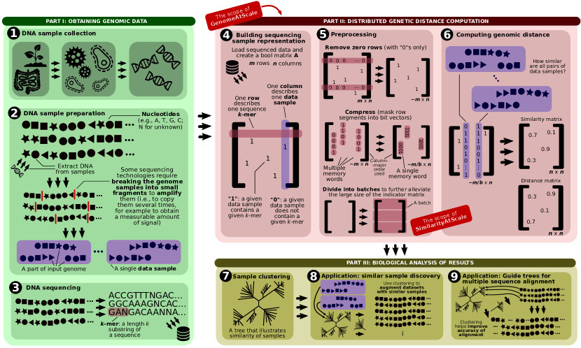
Figure 1: The scope of the SimilarityAtScale algorithm and GenomeAtScale tool within a metagenomics project. DNA is sequenced and preprocessed before being deposited into a database (❶–❸). Given sequence data from several samples, a binary matrix $\bm{A}$ is constructed indicating which $k$-mers are present in which samples (❹). The matrix is divided into batches and pair-wise Jaccard similarities are computed (❺–❻). The results may then be used for downstream genomics analysis (❼–❾).

IV Implementation

We package the SimilarityAtScale algorithm as part of GenomeAtScale, a tool for fast distributed genetic distance computation. Figure 1 illustrates the integration of GenomeAtScale with general genomics and metagenomics projects. GenomeAtScale includes infrastructure to produce files with a sorted numerical representation for each data sample. Each processor is responsible for reading in a subset of these files, scanning through one batch at a time. Once the data is read-in, the SimilarityAtScale implementation performs preprocessing and parallel sparse matrix mutliplication.

To realize both preprocessing and sparse matrix multiplication, we use the Cyclops library [78]. Cyclops is a distributed-memory library that delivers routines for contraction and summation of sparse and dense tensors. The library also provides primitives for sparse input and transformation of data. Importantly, Cyclops enables the user to work with distributed vectors/matrices/tensors with arbitrary fixed-size element data-types, and to perform arbitrary elementwise operations on these data-types. This generality is supported via C++ templating, lambda functions, and constructs for algebraic structures such as monoids and semirings [75, 77]. Cyclops relieves the user of having to manually determine the matrix data distribution. Cyclops automatically distributes matrices over all processors using a processor grid. Each routine searches for an optimal processor grid with respect to communication costs and any additional overheads, such as data redistribution.

Listing 2 provides the pseudocode for our overall approach. We describe details of how preprocessing and similarity calculation are done with Cyclops below.

IV-A Implementation of Preprocessing

After obtaining genome data (Part I), we load the input sequence files (using the established FASTA format [60]) and construct a sparse representation of the indicator matrix $\mathbf{A}$. The readFiles() function then processes the input data, and writes into a Cyclops sparse vector f, i.e., each $k$-mer is treated as an index to update f with $1$. To do this, we leverage the Cyclops write() function, which collects arbitrary inputs from all processes, combining them by accumulation, as specified by the algebraic structure associated with the tensor. We make use of the $(\max,\times)$ semiring for f so that each vector entry is 1 if any processor writes 1 to it.

Our implementation then proceeds by collecting the sparse vector f on all processors, and performing a local prefix sum to determine appropriate nonzero rows for each data item. This approach has been observed to be most efficient for the scale of problems that we consider in the experimental section. The use of the Cyclops read() function in place of replication would yield an implementation that matches the algorithm description and communication cost. The function preprocessInput() then proceeds to map the locally stored entries to nonzero rows as prescribed by the prefix sum of the filter and to apply the masking. The distributed Cyclops matrix storing the batch of the indicator matrix $\bm{\bar{A}}^{(l)}$ is then created by a call to write() from each processor with the nonzero entries it generates.

IV-B Implementation of Semiring Sparse Matrix Multiplication

Given the generated sparse matrix $\bm{\bar{A}}^{(l)}$, which corresponds to A in our pseudocode, the function jaccardAccumulate() proceeds to compute the contribution to $\bm{B}$. To do this with Cyclops, we define a dense distributed matrix B, and use the Einstein summation syntax provided by Cyclops to specify the matrix-multiplication. The use of the appropriate elementwise operation is specified via a Cyclops Kernel construct, which accepts an elementwise function for multiplication (for us popcount, which counts number of set bits via a hardware-supported routine) and another function for addition, which in our case is simply the addition of 64-bit integers. The Einstein summation notation with this kernel is used as follows

⬇

Jaccard_Kernel(A["ki"],A["kj"],B["ij"]);

Aside from this sparse matrix multiplication, it suffices to compute a column-wise summation of the matrix A, which is done using similar Cyclops constructs.

The resulting implementation of sparse matrix product is fully parallel, and can leverage 3D sparse matrix multiplication algorithms. The $\sqrt{p/c}\times\sqrt{p/c}\times c$ processor grid proposed in Section III-C can be delivered by Cyclops. Our results (almost ideal scaling) confirm that the desired scaling is achieved for the considered parameters’ spectrum.

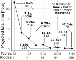
(a) Kingsford dataset, strong scaling.

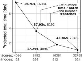
(b) BIGSI dataset, strong scaling.

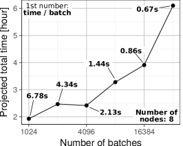
(c) Kingsford dataset, sensitivity analysis.

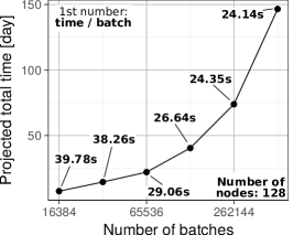
(d) BIGSI dataset, sensitivity analysis.

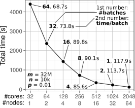
(e) Synthetic dataset, strong scaling.

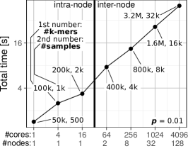
(f) Synthetic dataset, weak scaling.

Figure 2: Performance analysis of GenomeAtScale. We calculate 95% confidence intervals for the reported mean values by assuming the batch times are normally distributed samples. The derived confidence intervals are very tight around the means, and we exclude them from the plot to ensure clarity. The confidence values for the BIGSI dataset are 0.12 (for 128 nodes), 0.16 (for 256 nodes), 0.38 (for 512 nodes), and 0.40 (for 1024 nodes).

V Evaluation

We now analyze the performance of our implementation of SimilarityAtScale for real and synthetic datasets.

V-A Methodology and Setup

We first provide information that is required for interpretability and reproducibility [46].

V-A1 Experimental Setup

We use the Stampede2 supercomputer. Each node has a Intel Xeon Phi 7250 CPU (“Knights Landing”) with 68 cores, 96GB of DDR4 RAM, and 16GB of high-speed on-chip MCDRAM memory (which operates as 16GB direct-mapped L3). There is also 2KB of L1 data cache per core and 1MB of L2 per two-core tile. There are 4,200 compute nodes in total. The network is a fat tree with six core switches, with the 100 Gb/sec Intel Omni-Path architecture.

In our experiments, we consistently use 32 MPI processes per node. Using fewer processes per node enables larger batch sizes as our implementation replicates the filter vector on each processor. We also find that this configuration outperforms those with 64 processes per node for representative experiments, as the on-node computational kernels are generally memory-bandwidth bound. To maximize fair evaluation, we include the I/O time (loading data from disk) in the reported runtimes (the I/O time is $\approx$1% of the total runtime).

V-A2 Considered Real Datasets

We evaluate our design on datasets of differing sequence variability to demonstrate its scalability in different settings. As a low-variability set, we use the public BBB/Kingsford dataset consisting of 2,580 RNASeq experiments sequenced from human blood, brain, and breast samples [73] with sequencing reads of length at least 20. We consider all such experiments that were publicly available at the time of study. The raw sequences were preprocessed to remove rare (considered noise) $k$-mers. Minimum $k$-mer count thresholds were set based on the total sizes of the raw sequencing read sets [73]. We used the $k$-mer size of $19$ (unlike the value of $20$ used in [73]) to avoid the possibility of $k$-mers being equal to their reverse complements. As a high-variability set, we use all bacterial and viral whole-genome sequencing data used in the BIGSI database [21], representing almost every such experiment available as of its release, totaling 446,506 samples (composed overwhelmingly of Illumina short-read sequencing experiments). In the same fashion as the BIGSI, these data were preprocessed by considering longer contiguous stretches of $k$-mers to determine $k$-mer count thresholds [21]. We used the same $k$-mer size as the BIGSI paper ($k=31$).

The considered real datasets enable analyzing the performance of our schemes for different data sparsities. The indicator matrix $\bm{A}$ in the Kingsford dataset has a density of $\approx$$1.5\cdot 10^{-4}$, and in the BIGSI dataset its density is $\approx$$4\cdot 10^{-12}$. All input data is provided in the FASTA format [60].

V-A3 Considered Synthetic Datasets

We also use synthetic datasets where each element of the indicator matrix $\bm{A}$ is present with a specified probability $p$ (which corresponds to density), independently for all elements. This enables a systematic analysis of the impact of data sparsity on the performance of our schemes.

V-A4 Considered Scaling Scenarios

To illustrate the versatility of our design, we consider (1) strong scaling for a small dataset (fixed indicator matrix ($\bm{A}$) size, increasing batch size and core count), (2) strong scaling for a large dataset (same as above), (3) weak scaling (increasing the $\bm{A}$ size with core count, increasing batch size with core count), (4) batch size sensitivity (fixed node count, increasing batch size).

V-B Performance Analysis for Real Data

The results for the Kingsford and the BIGSI datasets are presented in Figure 2a and 2b, respectively. The BIGSI dataset as noted has $n=446,506$ columns. This requires us to distribute three matrices $\bm{A}$, $\bm{B}$, and $\bm{C}$ among the processes for the similarity calculation. We find it necessary to use 64 nodes to have enough memory to store these matrices. Hence, we report performance numbers for 128, 256, 512, and 1024 nodes. As we double the number of nodes, we also double the batch size, utilizing all available memory. We also use not more than 256 nodes for preprocessing, i.e., the sparse vector is constructed using not more than 256 nodes, but is used by all the participating nodes in the later stages of the pipeline. We find less variability in performance with this variant.

In Figure 2b, we show the average batch time (averaged across eight batches, not considering the first three batches to account for startup cost). Per batch time across nodes, remains the same (the batch size though is doubled according to the node size). The y-axis shows the predicted completion time for running the entire dataset to calculate the similarity matrix. We note that we are able to calculate the similarity matrix for BIGSI benchmark in a day (24.95 hours) using 1024 nodes. We note that despite high-variability of density across different columns in the BIGSI dataset, SimilarityAtScale achieves a good parallel efficiency even when using 32K cores.

Similarly, in Figure 2a, we show the results for the Kingsford dataset which is denser than BIGSI. The performance behavior observed for this smaller dataset is a bit less consistent. We observe both superscalar speed-ups and some slow-downs when increasing node count. On 32 nodes, we note a sweet-spot, achieving a 42.2$\times$ speed-up relative to the single node performance. Thus, we are able to construct the similarity matrix in less than an hour using 32 nodes. For larger node counts, the number of MPI processes (2048, 4096, 8192) starts to exceed the number of columns in the matrix (2,580), leading to load imbalance and deteriorating performance.

To verify the projected execution times, we fully process Kingsford for 128 nodes and 64 batches (we cannot derive data for all parameter values due to budget constraints). The total runtime takes 0.38h, the corresponding projection is 0.42h.

In Figures 2c and 2d, we show the sensitivity of the datasets for the size of the batches. For both datasets we observe a general trend that the execution time does not scale with batch size, despite the work scaling linearly with batch size. This behavior is expected, as a larger batch size has a lesser overhead in synchronization/latency and bandwidth costs, enabling a higher rate of performance. Thus, in both the datasets the overall projected time for the similarity matrix calculation reduces with the increase in batch size.

V-C Performance Analysis for Synthetic Data

In Figure 2e, we present the strong scaling results (with the increasing batch size) for synthetic data. The total time decreases in proportion to the node count, although the time per batch slightly increases, yielding good overall parallel efficiency, as predicted in our theoretical analysis. In Figure 2f, we show weak scaling by increasing the $\bm{A}$ matrix size and the batch size with the core count. In this weak scaling regime, the amount of work per processor is increasing with the node count. From 1 core to 4096 cores, the amount of work per processor increases by 64$\times$, while the execution time increases by 35.3$\times$, corresponding to a 1.81$\times$ efficiency improvement.

We also show how the performance for synthetic datasets changes with data sparsity expressed with the probability $p$ of the occurrence of a particular $k$-mer. The results are in Figure 3. We enable nearly ideal scaling of the total runtime with the decreasing data sparsity (i.e., with more data to process).

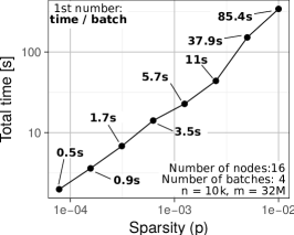
Figure 3: The impact of data sparsity on the performance of GenomeAtScale.

V-D Impact from Fast Cache

We also test our design without using MCDRAM as L3 cache, but instead as an additional memory storage. The resulting performance patterns are negligibly worse than the ones in which MCDRAM serves as L3. For example, time per batch with MCDRAM as L3 for Kingsford dataset on 4 nodes and 32 nodes is 9.26s and 7.69s, respectively. Then, without MCDRAM L3 cache, it is 9.33s and 8.01s, respectively.

VI Discussion and Related Work

The algebraic formulation of our schemes is generic and can be implemented with other frameworks such as CombBLAS [24, 51]. We selected Cyclops which is – to the best of our knowledge – the only library with high-performance routines where the input matrices are sparse but the outcome of the matrix-matrix multiplication is dense. CombBLAS targets primarily graph processing and, to the best of our knowledge, does not provide a fast implementation of matrix-matrix product with a dense output. Thus, CombBLAS would result in suboptimal performance when combined with SimilarityAtScale. One could also use MapReduce [32] and engines such as Spark [90] or Hadoop [87]. Yet, they are communication-intensive and their limited expressiveness often necessitates multiple communication rounds, resulting in inherent overheads when compared to communication-avoiding and expressive algebraic routines provided by Cyclops.

A recent closely related work, BELLA [44, 35], is the first to express similarity calculation for genetic sequences as sparse matrix-matrix multiplication. BELLA leverages parallel multiplication of sparse matrices for the computation of pairwise overlaps between long reads as a part of genome assembly [39, 27, 38, 42, 41, 34, 40] via Overlap Layout Consensus (OLC) [30]. BELLA constructs an overlap graph of reads in a read set while we target whole genome comparison, computing distances between entire read sets.

BELLA performs overlap detection using a sparse matrix multiplication $\bm{A}\bm{A}^{T}$, where $k$-mers correspond to columns of $\bm{A}$, and each row corresponds to a read. The data samples in BELLA are individual reads from the same read set (e.g., organism), while we consider all $k$-mers in a read set (e.g., corresponding to a whole genome) to constitute a single sample. In our context, $\bm{A}$ has many more nonzeros and more potential variability in density among columns. Further, the output Jaccard matrix is generally dense, while for BELLA the overlap is frequently zero. This fact has also motivated a specialized parallelization of the overlap and alignment calculations for BELLA [35], which are not based on parallel sparse matrix multiplication. Additionally, SimilarityAtScale employs parallel methods for compressing the input data, and the output matrix is computed in batches with the input matrix also constructed in batches, which are not necessary in the context of long reads in BELLA.

VII Conclusion

We introduce SimilarityAtScale, the first high-performance distributed algorithm for computing the Jaccard similarity, which is widely used in data analytics. SimilarityAtScale is based on an algebraic formulation that uses (1) provably communication-efficient linear algebra routines, (2) compression based on bitmasking, (3) batched computation to alleviate large input sizes, and (4) theoretical analysis that illustrates scalability in communication cost and parallel efficiency. The result is a generic high-performance algorithm that can be applied to any problem in data analytics that relies on Jaccard measures. To facilitate the utilization of SimilarityAtScale in different domains, we provide a comprehensive overview of problems that could be accelerated and scaled with our design.

We then use SimilarityAtScale as a backend to develop GenomeAtScale, the first tool for accurate large-scale calculations of distances between high-throughput whole-genome sequencing samples on distributed-memory systems. To foster DNA research, we use real established datasets in our evaluation, showing that – for example – GenomeAtScale enables analyzing all the bacterial and viral whole-genome sequencing data used in the BIGSI database in less than a day. We maintain compatibility with standard bioinformatics data formats, enabling seamless integration of GenomeAtScale with existing biological analysis pipelines. We conduct largest-scale exact computations of Jaccard genetic distances so far. Our publicly available design and implementation can be used to foster further research into DNA and general data analysis.

References

- [1] S. F. Altschul, W. Gish, W. Miller, E. W. Myers, and D. J. Lipman. Basic local alignment search tool. Journal of molecular biology, 215(3):403–410, 1990.
- [2] J. Armstrong, G. Hickey, M. Diekhans, A. Deran, Q. Fang, D. Xie, S. Feng, J. Stiller, D. Genereux, J. Johnson, V. D. Marinescu, D. Haussler, J. Alföldi, K. Lindblad-Toh, E. Karlsson, G. Zhang, and B. Paten. Progressive alignment with Cactus: a multiple-genome aligner for the thousand-genome era. bioRxiv, 2019.
- [3] A. Azad, G. Ballard, A. Buluç, J. Demmel, L. Grigori, O. Schwartz, S. Toledo, and S. Williams. Exploiting multiple levels of parallelism in sparse matrix-matrix multiplication. SIAM Journal on Scientific Computing, 38(6):C624–C651, 2016.
- [4] G. Ballard, A. Buluç, J. Demmel, L. Grigori, B. Lipshitz, O. Schwartz, and S. Toledo. Communication optimal parallel multiplication of sparse random matrices. In Proceedings of the Twenty-fifth Annual ACM Symposium on Parallelism in Algorithms and Architectures, SPAA ’13, pages 222–231, New York, NY, USA, 2013. ACM.
- [5] G. Ballard, J. Demmel, O. Holtz, and O. Schwartz. Minimizing communication in linear algebra. SIAM J. Mat. Anal. Appl., 32(3), 2011.
- [6] J. Bank and B. Cole. Calculating the Jaccard similarity coefficient with map reduce for entity pairs in wikipedia. Wikipedia Similarity Team, pages 1–18, 2008.
- [7] R. J. Bayardo, Y. Ma, and R. Srikant. Scaling up all pairs similarity search. In Proceedings of the 16th international conference on World Wide Web, pages 131–140. ACM, 2007.
- [8] T. Ben-Nun, M. Besta, S. Huber, A. N. Ziogas, D. Peter, and T. Hoefler. A modular benchmarking infrastructure for high-performance and reproducible deep learning. arXiv preprint arXiv:1901.10183, 2019.
- [9] M. Besta et al. Slim graph: Practical lossy graph compression for approximate graph processing, storage, and analytics. 2019.
- [10] M. Besta, M. Fischer, T. Ben-Nun, J. De Fine Licht, and T. Hoefler. Substream-centric maximum matchings on fpga. In ACM/SIGDA FPGA, pages 152–161, 2019.
- [11] M. Besta, M. Fischer, V. Kalavri, M. Kapralov, and T. Hoefler. Practice of streaming and dynamic graphs: Concepts, models, systems, and parallelism. arXiv preprint arXiv:1912.12740, 2019.
- [12] M. Besta and T. Hoefler. Accelerating irregular computations with hardware transactional memory and active messages. In ACM HPDC, 2015.
- [13] M. Besta and T. Hoefler. Active access: A mechanism for high-performance distributed data-centric computations. In ACM ICS, 2015.
- [14] M. Besta and T. Hoefler. Survey and taxonomy of lossless graph compression and space-efficient graph representations. arXiv preprint arXiv:1806.01799, 2018.
- [15] M. Besta, F. Marending, E. Solomonik, and T. Hoefler. Slimsell: A vectorizable graph representation for breadth-first search. In IEEE IPDPS, pages 32–41, 2017.
- [16] M. Besta, E. Peter, R. Gerstenberger, M. Fischer, M. Podstawski, C. Barthels, G. Alonso, and T. Hoefler. Demystifying graph databases: Analysis and taxonomy of data organization, system designs, and graph queries. arXiv preprint arXiv:1910.09017, 2019.
- [17] M. Besta, M. Podstawski, L. Groner, E. Solomonik, and T. Hoefler. To push or to pull: On reducing communication and synchronization in graph computations. In ACM HPDC, 2017.
- [18] M. Besta, D. Stanojevic, J. D. F. Licht, T. Ben-Nun, and T. Hoefler. Graph processing on fpgas: Taxonomy, survey, challenges. arXiv preprint arXiv:1903.06697, 2019.
- [19] M. Besta, D. Stanojevic, T. Zivic, J. Singh, M. Hoerold, and T. Hoefler. Log (graph): a near-optimal high-performance graph representation. In PACT, pages 7–1, 2018.
- [20] I. Binanto, H. L. H. S. Warnars, B. S. Abbas, Y. Heryadi, N. F. Sianipar, and H. E. P. Sanchez. Comparison of similarity coefficients on morphological rodent tuber. In 2018 Indonesian Association for Pattern Recognition International Conference (INAPR), pages 104–107. IEEE, 2018.
- [21] P. Bradley, H. C. den Bakker, E. P. Rocha, G. McVean, and Z. Iqbal. Ultrafast search of all deposited bacterial and viral genomic data. Nature biotechnology, 37(2):152, 2019.
- [22] B. Brekhna, C. Zhang, and Y. Zhou. An experimental approach for evaluating superpixel’s consistency over 2D Gaussian blur and impulse noise using Jaccard similarity coefficient. International Journal of Computer Science and Security (IJCSS), 13(3):53, 2019.
- [23] A. Buluç and J. R. Gilbert. On the representation and multiplication of hypersparse matrices. In 2008 IEEE International Symposium on Parallel and Distributed Processing, pages 1–11. IEEE, 2008.
- [24] A. Buluç and J. R. Gilbert. The Combinatorial BLAS: Design, implementation, and applications. The International Journal of High Performance Computing Applications, 25(4):496–509, 2011.
- [25] A. Buluç and J. R. Gilbert. Parallel sparse matrix-matrix multiplication and indexing: Implementation and experiments. SIAM Journal on Scientific Computing, 34(4):C170–C191, 2012.
- [26] P. Burkhardt. Asking hard graph questions. US National Security Agency Technical report NSA-RD-2014-050001v1, 2014.
- [27] J. A. Chapman, M. Mascher, A. Buluç, K. Barry, E. Georganas, A. Session, V. Strnadova, J. Jenkins, S. Sehgal, L. Oliker, et al. A whole-genome shotgun approach for assembling and anchoring the hexaploid bread wheat genome. Genome biology, 16(1):26, 2015.
- [28] H.-H. Chen, L. Gou, X. L. Zhang, and C. L. Giles. Discovering missing links in networks using vertex similarity measures. In Proceedings of the 27th annual ACM symposium on applied computing, pages 138–143. ACM, 2012.
- [29] I. Choi, A. J. Ponsero, M. Bomhoff, K. Youens-Clark, J. H. Hartman, and B. L. Hurwitz. Libra: scalable k-mer–based tool for massive all-vs-all metagenome comparisons. GigaScience, 8(2):giy165, 2018.
- [30] J. Chu, H. Mohamadi, R. L. Warren, C. Yang, and I. Birol. Innovations and challenges in detecting long read overlaps: an evaluation of the state-of-the-art. Bioinformatics, 33(8):1261–1270, 2016.
- [31] M. Cosulschi, M. Gabroveanu, F. Slabu, and A. Sbircea. Scaling up a distributed computing of similarity coefficient with MapReduce. IJCSA, 12(2):81–98, 2015.
- [32] J. Dean and S. Ghemawat. MapReduce: simplified data processing on large clusters. Communications of the ACM, 51(1):107–113, 2008.
- [33] Y. Dong, Y. Zhuang, K. Chen, and X. Tai. A hierarchical clustering algorithm based on fuzzy graph connectedness. Fuzzy Sets and Systems, 157(13):1760–1774, 2006.
- [34] M. Ellis, E. Georganas, R. Egan, S. Hofmeyr, A. Buluç, B. Cook, L. Oliker, and K. Yelick. Performance characterization of de novo genome assembly on leading parallel systems. In European Conference on Parallel Processing, pages 79–91. Springer, 2017.
- [35] M. Ellis, G. Guidi, A. Buluç, L. Oliker, and K. Yelick. diBELLA: Distributed long read to long read alignment. In 48th International Conference on Parallel Processing (ICPP), Kyoto, Japan, 2019.
- [36] A. Fender, N. Emad, S. Petiton, J. Eaton, and M. Naumov. Parallel Jaccard and related graph clustering techniques. In Proceedings of the 8th Workshop on Latest Advances in Scalable Algorithms for Large-Scale Systems, page 4. ACM, 2017.
- [37] R. Ferdous et al. An efficient k-means algorithm integrated with Jaccard distance measure for document clustering. In 2009 First Asian Himalayas International Conference on Internet, pages 1–6. IEEE, 2009.
- [38] E. Georganas, A. Buluç, J. Chapman, S. Hofmeyr, C. Aluru, R. Egan, L. Oliker, D. Rokhsar, and K. Yelick. Hipmer: an extreme-scale de novo genome assembler. In Proceedings of the International Conference for High Performance Computing, Networking, Storage and Analysis, page 14. ACM, 2015.
- [39] E. Georganas, A. Buluç, J. Chapman, L. Oliker, D. Rokhsar, and K. Yelick. Parallel de bruijn graph construction and traversal for de novo genome assembly. In SC’14: Proceedings of the International Conference for High Performance Computing, Networking, Storage and Analysis, pages 437–448. IEEE, 2014.
- [40] E. Georganas, R. Egan, S. Hofmeyr, E. Goltsman, B. Arndt, A. Tritt, A. Buluç, L. Oliker, and K. Yelick. Extreme scale de novo metagenome assembly. In SC18: International Conference for High Performance Computing, Networking, Storage and Analysis, pages 122–134. IEEE, 2018.
- [41] E. Georganas, M. Ellis, R. Egan, S. Hofmeyr, A. Buluç, B. Cook, L. Oliker, and K. Yelick. Merbench: Pgas benchmarks for high performance genome assembly. In Proceedings of the Second Annual PGAS Applications Workshop, page 5. ACM, 2017.
- [42] E. Georganas, S. Hofmeyr, L. Oliker, R. Egan, D. Rokhsar, A. Buluc, and K. Yelick. Extreme-scale de novo genome assembly. Exascale Scientific Applications: Scalability and Performance Portability, page 409, 2017.
- [43] L. Gianinazzi, P. Kalvoda, A. De Palma, M. Besta, and T. Hoefler. Communication-avoiding parallel minimum cuts and connected components. In ACM SIGPLAN Notices, volume 53, pages 219–232. ACM, 2018.
- [44] G. Guidi, M. Ellis, D. Rokhsar, K. Yelick, and A. Buluç. BELLA: Berkeley efficient long-read to long-read aligner and overlapper. bioRxiv, page 464420, 2019.
- [45] F. G. Gustavson. Two fast algorithms for sparse matrices: Multiplication and permuted transposition. ACM Transactions on Mathematical Software (TOMS), 4(3):250–269, 1978.
- [46] T. Hoefler and R. Belli. Scientific benchmarking of parallel computing systems: twelve ways to tell the masses when reporting performance results. In Proceedings of the international conference for high performance computing, networking, storage and analysis, page 73. ACM, 2015.
- [47] T. Hoefler and D. Moor. Energy, memory, and runtime tradeoffs for implementing collective communication operations. Supercomputing frontiers and innovations, 1(2):58–75, 2014.
- [48] X. Hu, K. Yi, and Y. Tao. Output-optimal massively parallel algorithms for similarity joins. ACM Transactions on Database Systems (TODS), 44(2):6, 2019.
- [49] P. Jaccard. Étude comparative de la distribution florale dans une portion des alpes et des jura. Bull Soc Vaudoise Sci Nat, 37:547–579, 1901.
- [50] R. A. Jarvis and E. A. Patrick. Clustering using a similarity measure based on shared near neighbors. IEEE Transactions on computers, 100(11):1025–1034, 1973.
- [51] J. Kepner, P. Aaltonen, D. Bader, A. Buluç, F. Franchetti, J. Gilbert, D. Hutchison, M. Kumar, A. Lumsdaine, H. Meyerhenke, et al. Mathematical foundations of the graphblas. In 2016 IEEE High Performance Extreme Computing Conference (HPEC), pages 1–9. IEEE, 2016.
- [52] P. Koanantakool, A. Azad, A. Buluç, D. Morozov, S.-Y. Oh, L. Oliker, and K. Yelick. Communication-avoiding parallel sparse-dense matrix-matrix multiplication. In Parallel and Distributed Processing Symposium, 2016 IEEE International, pages 842–853. IEEE, 2016.
- [53] P. M. Kogge. Jaccard coefficients as a potential graph benchmark. In 2016 IEEE International Parallel and Distributed Processing Symposium Workshops (IPDPSW), pages 921–928. IEEE, 2016.
- [54] S. Kosub. A note on the triangle inequality for the Jaccard distance. Pattern Recognition Letters, 120:36–38, 2019.
- [55] V. Kotu and B. Deshpande. Data Science: Concepts and Practice. Morgan Kaufmann, 2018.
- [56] G. P. Krawezik, P. M. Kogge, T. J. Dysart, S. K. Kuntz, and J. O. McMahon. Implementing the Jaccard index on the migratory memory-side processing Emu architecture. In 2018 IEEE High Performance extreme Computing Conference (HPEC), pages 1–6. IEEE, 2018.
- [57] G. Kucherov. Evolution of biosequence search algorithms: a brief survey. Bioinformatics, 35(19):3547–3552, 2019.
- [58] G. Kwasniewski, M. Kabić, M. Besta, J. VandeVondele, R. Solcà, and T. Hoefler. Red-blue pebbling revisited: near optimal parallel matrix-matrix multiplication. In ACM/IEEE Supercomputing, page 24. ACM, 2019.
- [59] M. Levandowsky and D. Winter. Distance between sets. Nature, 234(5323):34, 1971.
- [60] D. J. Lipman and W. R. Pearson. Rapid and sensitive protein similarity searches. Science, 227(4693):1435–1441, 1985.
- [61] T. Morzy, M. Wojciechowski, and M. Zakrzewicz. Scalable hierarchical clustering method for sequences of categorical values. In Pacific-Asia Conference on Knowledge Discovery and Data Mining, pages 282–293. Springer, 2001.
- [62] R. Moulton and Y. Jiang. Maximally consistent sampling and the Jaccard index of probability distributions. arXiv preprint arXiv:1809.04052, 2018.
- [63] B. D. Ondov, T. J. Treangen, P. Melsted, A. B. Mallonee, N. H. Bergman, S. Koren, and A. M. Phillippy. Mash: fast genome and metagenome distance estimation using MinHash. Genome biology, 17(1):132, 2016.
- [64] V. Popic, V. Kuleshov, M. Snyder, and S. Batzoglou. Fast metagenomic binning via hashing and bayesian clustering. Journal of Computational Biology, 25(7):677–688, 2018.
- [65] H. Rezatofighi, N. Tsoi, J. Gwak, A. Sadeghian, I. Reid, and S. Savarese. Generalized intersection over union: A metric and a loss for bounding box regression. In Proceedings of the IEEE Conference on Computer Vision and Pattern Recognition, pages 658–666, 2019.
- [66] V. Sachdeva, D. M. Freimuth, and C. Mueller. Evaluating the Jaccard-Tanimoto index on multi-core architectures. In International Conference on Computational Science, pages 944–953. Springer, 2009.
- [67] N. Saitou and M. Nei. The neighbor-joining method: a new method for reconstructing phylogenetic trees. Molecular biology and evolution, 4(4):406–425, 1987.
- [68] S. E. Schaeffer. Graph clustering. Computer science review, 1(1):27–64, 2007.
- [69] J. Scripps and C. Trefftz. Parallelizing an algorithm to find communities using the Jaccard metric. In 2015 IEEE International Conference on Electro/Information Technology (EIT), pages 370–372. IEEE, 2015.
- [70] D. Selivanov and Q. Wang. text2vec: Modern text mining framework for r. Computer software manual (R package version 0.4. 0), 2016.
- [71] S. Seth, N. Välimäki, S. Kaski, and A. Honkela. Exploration and retrieval of whole-metagenome sequencing samples. Bioinformatics, 30(17):2471–2479, 2014.
- [72] D. B. Skillicorn, J. Hill, and W. F. McColl. Questions and answers about BSP. Scientific Programming, 6(3):249–274, 1997.
- [73] B. Solomon and C. Kingsford. Fast search of thousands of short-read sequencing experiments. Nature biotechnology, 34(3):300, 2016.
- [74] E. Solomonik, M. Besta, F. Vella, and T. Hoefler. Scaling betweenness centrality using communication-efficient sparse matrix multiplication. In ACM/IEEE Supercomputing, page 47, 2017.
- [75] E. Solomonik, M. Besta, F. Vella, and T. Hoefler. Scaling betweenness centrality using communication-efficient sparse matrix multiplication. In Proceedings of the International Conference for High Performance Computing, Networking, Storage and Analysis, SC ’17, pages 47:1–47:14, 2017.
- [76] E. Solomonik and J. Demmel. Communication-optimal parallel 2.5D matrix multiplication and LU factorization algorithms. In Euro-Par 2011 Parallel Processing, volume 6853 of Lecture Notes in Computer Science, pages 90–109. 2011.
- [77] E. Solomonik and T. Hoefler. Sparse tensor algebra as a parallel programming model. arXiv preprint arXiv:1512.00066, 2015.
- [78] E. Solomonik, D. Matthews, J. R. Hammond, J. F. Stanton, and J. Demmel. A massively parallel tensor contraction framework for coupled-cluster computations. Journal of Parallel and Distributed Computing, 74(12):3176–3190, 2014.
- [79] Z. D. Stephens, S. Y. Lee, F. Faghri, R. H. Campbell, C. Zhai, M. J. Efron, R. Iyer, M. C. Schatz, S. Sinha, and G. E. Robinson. Big data: Astronomical or genomical? PLoS Biology, 2015.
- [80] A. Strehl, J. Ghosh, and R. Mooney. Impact of similarity measures on web-page clustering. In Workshop on artificial intelligence for web search (AAAI 2000), volume 58, page 64, 2000.
- [81] P.-N. Tan, M. Steinbach, A. Karpatne, and V. Kumar. Introduction to data mining, 2018.
- [82] S. Theodoridis and K. Koutroumbas. Pattern recognition. 2003. Elsevier Inc, 2009.
- [83] E. Valari and A. N. Papadopoulos. Continuous similarity computation over streaming graphs. In Joint European Conference on Machine Learning and Knowledge Discovery in Databases, pages 638–653. Springer, 2013.
- [84] L. G. Valiant. A bridging model for parallel computation. Communications of the ACM, 33(8):103–111, 1990.
- [85] R. A. Van De Geijn and J. Watts. SUMMA: Scalable Universal Matrix Multiplication Algorithm. Concurrency: Practice and Experience, 9(4):255–274, 1997.
- [86] R. Vernica, M. J. Carey, and C. Li. Efficient parallel set-similarity joins using MapReduce. In Proceedings of the 2010 ACM SIGMOD International Conference on Management of data, pages 495–506. ACM, 2010.
- [87] T. White. Hadoop: The Definitive Guide. O’Reilly Media, Inc., 1st edition, 2009.
- [88] D. E. Wood and S. L. Salzberg. Kraken: ultrafast metagenomic sequence classification using exact alignments. Genome biology, 15(3):R46, 2014.
- [89] Z. Wu. Service Computing: Concept, Method and Technology. Academic Press, 2014.
- [90] M. Zaharia, M. Chowdhury, M. J. Franklin, S. Shenker, and I. Stoica. Spark: Cluster computing with working sets. HotCloud, 10(10-10):95, 2010.
- [91] K. Zhou, T. P. Michalak, M. Waniek, T. Rahwan, and Y. Vorobeychik. Attacking similarity-based link prediction in social networks. In Proceedings of the 18th International Conference on Autonomous Agents and MultiAgent Systems, pages 305–313. International Foundation for Autonomous Agents and Multiagent Systems, 2019.
- [92] A. Zielezinski, S. Vinga, J. Almeida, and W. M. Karlowski. Alignment-free sequence comparison: benefits, applications, and tools. Genome biology, 18(1):186, 2017.