Quantitative earnings enhancement from share buybacks

Abstract

This paper aims to explore the mechanical effect of a company’s share repurchase on earnings per share (EPS). In particular, while a share repurchase scheme will reduce the overall number of shares, suggesting that the EPS may increase, clearly the expenditure will reduce the net earnings of a company, introducing a trade-off between these competing effects. We first of all review accretive share repurchases, then characterise the increase in EPS as a function of price paid by the company. Subsequently, we analyse and quantify the estimated difference in earnings growth between a company’s natural growth in the absence of buyback scheme to that with its earnings altered as a result of the buybacks. We conclude with an examination of the effect of share repurchases in two cases studies in the US stock-market. Accompanying code can be found at https://github.com/particlemontecarlo/quantifying_eps_buybacks.

1 Introduction

1.1 Share repurchases background

Share repurchases provide a popular means for companies to return cash to their shareholders as an alternative to stock dividends [12, 13]. Popularised in the 80s, following a change in regulations governing open market share repurchase schemes, they became a means for managers to alter earnings per share via financial engineering [7, 4] thereby having a knock-on effect on the share price. Since, repurchase programs have generally increased in US stocks [6], with the value of buybacks of S&P 500 companies representing a significant portion of US gross domestic private investment. In general, the precise reasons for a company to buybacks its shares may vary [2], however efforts have shown that companies may use them as an earnings management device, with evidence to suggest the intention of aiming to inflate the earnings per share [11]. Indeed, while share repurchases inevitably reduce the number of shares outstanding (thereby reducing the divisor of the earnings per share), such an action will inevitably shrink a company’s asset base thereby potentially having a negative effect on the earnings per share [1].

From an investment perspective, on the one hand it may provide a positive sign that a company’s board believes in the future growth in the company - enough to treat the repurchase as an investment decision – on the other hand such a decision may also reflect that the company has limited investment opportunity (as well as the aforementioned motivation to inflate earnings) [8].

1.2 Share repurchases in the media

Recently, buybacks have made headlines due to a ‘record year’ in buybacks [10] and the recent activity following the very high level of cash reserves held by a number of companies, particularly in the technology sector, [16, 17] (curtailing only recently [9]), with similar activity observed in the aerospace industry [3]. A recent surge in US repurchases has been observed in part due to Trump’s tax reform thereby freeing up capital [15]. The FT article ‘Negative interest rates fuel record Japan share buybacks’ (May 24, 2016) remarks the increase buybacks as a result of negative interest rates in Japan. However, the surge in buyback activity has seen criticism in [5] as newly available cash reserves are spent on repurchases benefitting investors rather than boosting employment or R&D. Additionally, a correlation in [14] has been observed between the increase in sell-offs of single stocks and an increase in purchasing ETFs related to buybacks.

Figure 1.1 compares the amount spent on buybacks by the S&P 500 with a measure of interest in buybacks determined through Google trends - a measure of the number of Google searches worldwide. We see that there is a reasonable degree of correlation between the two; furthermore, there is a peak in search activity in mid 2018.

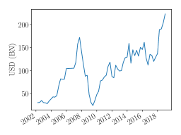
(a) Share buybacks on S&P 500

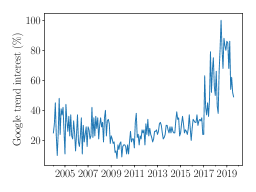
(b) Google interest index

Figure 1.1: Comparison of value of buybacks spent on S&P 500 since 2004 and interest measured by Google searches

1.3 Quantifying share repurchases

The following work aims to quantify explicitly how share repurchases can be used to mechanically inflate (or deflate) a company’s earnings per share. A method is developed through an argument based on cash flow analysis to examine how the buyback affects this, isolating a few unitless quantities relating to both the current prevailing state of the wider economy and a company’s characteristics, all of which can be obtained publicly, to quantify this effect. We primarily treat the earnings as growing geometrically, though provide an alternative analysis when the earnings are treated as growing arithmetically (providing a more rigorous quantification of the uncertainty) in the Appendix.

In addition we are able to explore the sensitivity of the growth in earnings to the changes in the salient variables. Finally, we are able use this analysis to estimate a company’s natural growth rate without this artificial inflation of the earnings. In particular, we focus on the US market, examining the S&P 500 and Apple as an individual stock as case studies.

2 Accretive share repurchases

We consider the effect on earnings as a consequence of share repurchases at different prices. With similar expressions remarked in the literature [11, 1], the following shows that the repurchase is accretive (increases the earnings per share) only if the price-earnings ratio, denoted $P_{E}$, of the traded company is less than a certain value dependent on the interest and tax rate ($i$ and $t_{\text{Tax}}$ respectively). Or, put another way, if the earnings yield (the reciprocal of the P/E ratio) is greater than the after tax interest rate earned on the company’s cash.

We have that the earning per share (for $N$ shares issued) for a company can be expressed as follows

$$E :=\text{Earnings per share}$$

$$=\frac{(O+Ci)(1-t_{\text{Tax}})-m_{min}}{N}$$

where $O$, $C$, and $m_{\text{min}}$ denote the trading profit, cash reserves and minority charge respectively. If the company spends $S$ to repurchase its shares at a price $P$, then with a dividend of $d$ the earnings per share after the repurchase, $E^{\prime}$, will be adjusted as follows

$$E^{\prime}=\frac{(O+\left(C-S\left(1+\frac{d}{P}\right)\right)i)(1-t_{\text{Tax}})-m_{min}}{N-\frac{S}{P}}$$

For the purposes of the following we assume that both the contribution from dividends is negligible, i.e $d\ll P$, and that the minority charge negligible, i.e. $m_{min}\approx 0$. Finally, we let $\alpha=1-t_{\text{Tax}}$ denote the fraction of assets retained after tax. As a result, for a repurchase to be accretive we require that $E^{\prime}\geq E$ and so

$$(O+\left(C-S\right)i)\alpha N \geq(O+Ci)\alpha\left(N-\frac{S}{P}\right)$$

$$(O+Ci)\alpha\frac{S}{P} \geq Si\alpha N$$

Which after rearrangement suggests that

$$\frac{(O+Ci)\alpha}{N}/P\geq i\alpha \implies P_{E}=\frac{P}{E}\leq\frac{1}{i\alpha}$$

i.e. the price-earnings ratio is less than $\frac{1}{i\alpha}$. We will, therefore, in the following refer to $P_{E}^{*}:=\frac{1}{\alpha i}$ as the ‘critical P-E ratio’ and $P^{*}:=\frac{E}{\alpha i}$ as the ‘critical price’ given a company’s earnings per share $E$. To ensure proper units, we note that the period over which a company’s earnings per share is stated must correspond to the period over which interest $i$ is paid. Unless otherwise stated, we assume that both time periods are annualised. Nominal values for the critical PE ratio are shown as a function of the interest rate $i\in[1\%,10\%]$ in Figure 3.1a and for value of tax rate between $10\%$ and $50\%$. We see that for interest rates between 2-3% with tax rates between 10-50% then the critical P/E is around 50.

Note that the long-term decline in interest rates over the last four decades has had the effect of increasing the the critical P-E ratio from approximately 15 in the late 1980’s to the current level of roughly 50 in the late 2010s. A corollary of this effect as we shall come on to quantify is that the boost to earnings per share for a given proportion of shares repurchased has increased significantly over the same period.

3 Earnings enhancement under buybacks

We are interested in how the earnings per share after a buyback (or sequence of buybacks) given the expenditure at time differs from that without a buyback. In the following we will consider under a geometric model for earnings growth what the natural earnings would look like given knowledge of the size of the buyback and quantities reflecting the state of the economy. For an interest rate of $i$ which we assume is approximately constant, we define a company’s earnings at time $t$ as

$$E_{t}=\alpha\frac{O_{t}+C_{t}i}{N_{t}}$$

where $O_{t}$ is operating earnings and $C_{t}$ is the net interest earning assets $\alpha=1-t_{\text{Tax}}$ which we assume is approximately constant. Additionally, we assume that $O_{t}$ is the same in both the presence and absence of a buyback. We model the interest earning assets as

$$C_{T}=C_{t}I_{t,T}$$

where $I_{t,T}$ is a continuously compounded interest rate process, for example, $I_{t,T}=(1+\imath)^{T-t}$ for some constant $\imath\geq 0$. Throughout, $T$ will be used to refer to a terminal index and $t$ an initial point in time (sometimes 0).

We let $\gamma_{t}:=\frac{S_{t}}{P_{t}N_{t}}$ denote the fraction paid of the market capitalisation in the buyback at time $t$ and $m_{t}:=\frac{P_{t}}{P_{t}^{*}}$ as the definition of the share price as a fraction of the critical price.

Proposition 1.

The difference in earnings at time $T$, $E_{T}^{\prime}$, relative to that without a buyback $E_{T}$ can be expressed as

$$E^{\prime}_{T}=\frac{E_{T}-m_{t}\gamma_{t}I_{t,T}E_{t}}{1-\gamma_{t}}$$ (3.1)

and we have the following approximation for the difference in earnings with and without buybacks as

$$E^{\prime}_{T} =E_{T}+\left(E_{T}-m_{t}I_{t,T}E_{t}\right)\sum_{n=1}^{\infty}\gamma_{t}^{n}$$

$$=E_{T}+\left(E_{T}-m_{t}I_{t,T}E_{t}\right)\gamma_{t}+\mathcal{O}(\gamma_{t}^{2})$$

Proof in Appendix.

We consider a simple example when the buyback is accretive so that $m_{t}\in[0,1]$. and, additionally, under a simple growth strategy where earnings at time $t$ are simply invested in a risk-free investment we have that $E_{T}=I_{t,T}E_{t}$. In this case we have that

$$\frac{E_{T}^{\prime}-E_{T}}{E_{T}}\geq\left(1-m_{t}\right)\gamma_{t}$$

So we see that we may increase the earnings at a future time $T$ in the presence of a buyback at time $t$ by an amount at least proportional to that spent on the buyback scheme $\gamma_{t}$. Such a relation provides a significant incentive for managers with pay related to earnings performance to increase the earnings per share through buying back shares, up to the extent that they are accretive. We explore this in more detail in the following.

3.1 Instantaneous enhancement under buybacks

We are able to consider the instantaneous change in earnings growth as a result of the buyback through setting $T=t$. As a result we see that by Proposition 1, that the earnings per share post-buyback can be expressed succinctly as

$$E^{\prime}=\frac{1-m\gamma}{1-\gamma}E$$

dependency of $m=\frac{P}{P^{*}}$ and $\gamma$ on $t$ is suppressed for notational convenience and we set $I_{t,t}=1$. Similarly, we have that the relative change is then

$$\Delta E:=\frac{E^{\prime}-E}{E} =\frac{\gamma}{1-\gamma}(1-m)$$ (3.2)

We see as expected, for zero expenditure ($\gamma=0$) then the change in earnings is 0. Furthermore, performing a series expansion of $\Delta E$ around $\gamma=0$, i.e. suggesting relative to the market capitalisation the amount spent on the repurchase by the company is small we have that up to an $o((m\gamma)^{2})$ term that

$$\Delta E\approx\left(\frac{1}{m}-1\right)m\gamma=\frac{S}{P^{*}N}\left(\frac{1}{m}-1\right)$$ (3.3)

In particular, if we further assume that the buyback is accretive, i.e. $P_{E}\leq P_{E}^{*}$, then we have that both $m,\gamma\in[0,1]$ and that the remainders in the series expansion are positive, suggesting that in fact $\Delta E\geq\frac{S}{P^{*}N}\left(\frac{1}{m}-1\right)$ so that the approximation is conservative in this sense. This linearisation shows how the relative change in earnings is affected as a function of the proportion spent on the critical price. The gains (or losses) of earnings as a result of the buyback under this normalisation are plotted in Figure 3.1 as a function of the price paid for the shares for both the exact expression 3.2 and the first order approximation 3.3. As can be seen, the linearisation is considerably accurate for $\frac{S}{P^{*}N}\approx 1\%$ and for a large range of $m$. We also see that the improvement to earnings rises quite steeply as $m$ approaches 0, demonstrative of the highly nonlinear relationship between the two.

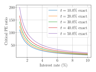
(a) Critical PE ratio $i\alpha=i(1-t_{\text{Tax}})$ as a function of interest rates.

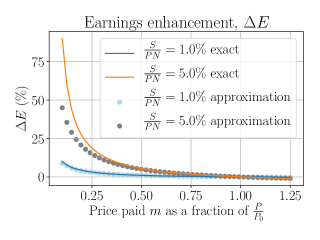
(b) Earnings enhancement $\Delta E$ in terms of price paid for repurchase.

Figure 3.1: Critical price and EPS enhancement

3.2 Earnings enhancement under geometric growth in earnings

We are now interested in the value of earnings at some future time $T$ given a buyback for $\gamma_{t}$ at time $t<T$. In the following, we let $E_{t}$ denote the natural earnings under the absence of a buyback scheme and define the normalised natural earnings $\hat{x}$ from time $t\geq 0$ to $T\geq t$ implicitly as satisfying

$$E_{T}=\hat{x}_{t,T}E_{t}$$

In this case we have that from Proposition 1 that

$$E_{T}^{\prime} =\frac{E_{T}-m_{t}\gamma_{t}I_{t,T}E_{t}}{1-\gamma_{t}}$$

$$=\frac{1}{1-\gamma_{t}}\left(E_{T}-I_{t,T}\frac{E_{t}}{P_{t}^{*}}\frac{S_{t}}{N_{t}}\right)$$

$$=\frac{1}{1-\gamma_{t}}\left(1-\frac{I_{t,T}}{\hat{x}_{t,T}}\frac{S_{t}}{P_{t}^{*}N_{t}}\right)E_{T}$$

Finally, substituting again $\gamma_{t}=\frac{S_{t}}{P_{t}N_{t}}$ as the proportion spent on share buybacks relative to the market capitalisation and substitute $P_{t}=mP_{t}^{*}$ we can express this neatly as

$$E_{T}^{\prime}=\frac{1}{1-\gamma_{t}}\left(1-m\gamma_{t}\frac{I_{t,T}}{\hat{x}_{t,T}}\right)E_{T}$$ (3.4)

We consider the special case of $t=0$ and simple constant geometric growth models both for interest rates and growth, i.e. that $\hat{x}_{0,T}=(1+\xi)^{T}$ and $I_{0,T}=(1+\imath)^{T}$ for two constants $\xi,\imath\geq 0$. In this case letting $\gamma$ denote the normalised value of the buyback at $t=0$ then

$$E_{T}^{\prime}=\frac{1}{1-\gamma}\left(1-m\gamma\left(\frac{1+\imath}{1+\xi}\right)^{T}\right)E_{T}$$

As we can see, if we consider the ‘immediate’ change in EPS by setting $T=0$, we recover the earnings enhancement as detailed above. Such a formula reveals a number of important characteristics of share buybacks. Firstly, to a degree as expected, as the interest rate $\imath$ increases the future enhancement diminishes, suggesting that the company would have been better retaining the cash rather than repurchasing shares, as measured by the earnings per share. Furthermore, we see that up to an $o(\gamma^{2})$ term then a series expansion of $E^{\prime}_{T}$ around $\gamma=0$ provides the approximation

$$\frac{E_{T}^{\prime}-E_{T}}{E_{T}}\approx\left(1-m\left(\frac{1+\imath}{1+\xi}\right)^{T}\right)\gamma.$$ (3.5)

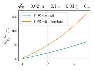
Figure 3.2: Example earnings enhancement over a period of 5 years, normalised by the initial earnings $E_{0}$.

We refer to the boost arising from buybacks to the earnings as ‘the earnings enhancement’. The series approximation of (3.5) is conservative in that the remainder is positive for $\gamma>0$. We explore nominal values of $\gamma$ in the next section. We note that provided $\xi>\imath$ the earnings enhancement converges exponentially towards $\lim_{T\rightarrow\infty}\left(1-m\left(\frac{1+\imath}{1+\xi}\right)^{T}\right)\gamma=\gamma$ through time suggesting that despite the initial cost in repurchasing the shares, the effect on the earnings can diminish relatively quickly through time.

We plot the EPS enhancement through time for some representative values of $m$, $x$ and $i$. Based on the current Federal Funds rate of $2\%$ we use this value for $i$. We then consider $x=0.1$ with $m=0.1$, i.e. an annual growth rate of $10\%$ and shares repurchased at $10\%$ of the critical price and $\frac{S}{P^{*}N}=2\%$. As will be seen, such values are representative of the buyback scheme undertaken by Apple since 2011/2012. For these two values of $m$ we compare $\frac{E_{T}^{\prime}-E_{0}}{E_{0}}$ with $\frac{E_{T}-E_{0}}{E_{0}}$, plotting the results in 3.2.

3.3 Earnings enhancement under buyback program

We here illustrate that under benign conditions (i.e. accretive buybacks) the growth in earnings increases geometrically on top of a geometric earnings growth as per the special case considered previously.

Consider the affect on earnings per share after a series of buybacks occurring at regular intervals. We have that at time $t$ after a buyback at time 0 that the earnings enhancement above the natural EPS at time $t$ can be expressed equivalently as

$$\Delta E_{t} =\frac{\gamma}{1-\gamma}\left(1-m\left(\frac{1+\imath}{1+\xi}\right)^{t}\right)$$

We consider a buyback program with repurchases occurring at intervals $t=cn$ for $n=1,2,...,T$ and $c>0$. In this case we see that

$$E_{n}^{\prime} =\prod_{k=0}^{n}(1+\Delta E(c(n-k)))E_{n}$$

$$=\prod_{k=0}^{n}\left(\frac{1}{1-\gamma}\left(1-m\gamma\left(\frac{1+\imath}{1+\xi}\right)^{c(n-k)}\right)\right)(1+\xi)^{cn}E_{0}$$

$$=\left(\frac{(1+\xi)^{c}}{1-\gamma}\right)^{n}\prod_{k=0}^{n}\left(1-m\gamma\left(\frac{1+\imath}{1+\xi}\right)^{c(n-k)}\right)E_{0}$$

$$=\left(\frac{(1+\xi)^{c}}{1-\gamma}\right)^{n}\prod_{k=0}^{n}\left(1-m\gamma\left(\frac{1+\imath}{1+\xi}\right)^{ck}\right)E_{0}$$ (3.6)

for low interest rates, i.e. $\xi\geq\imath$ we see that as $m,\gamma\in[0,1]$ then $\left(1-m\gamma\left(\frac{1+\imath}{1+\xi}\right)^{ck}\right)\geq\left(1-m\gamma\left(\frac{1+\imath}{1+\xi}\right)^{c}\right)$ as $k\geq 1$. We see that

$$\frac{E_{n}^{\prime}}{E_{0}} \geq\left(\frac{(1+\xi)^{c}}{1-\gamma}\right)^{n}\left(1-m\gamma\left(\frac{1+\imath}{1+\xi}\right)^{c}\right)^{n}$$

$$\geq(1+\xi)^{cn}\left(1+d\gamma\right)^{n}$$

where the inequality arises from a series approximation up to an $o(\gamma^{2})$ term, as before, with the constant $d$ independent of $\gamma$. In periods of low interest rate relative to company growth the increase in earnings per share resulting from a buyback scheme is at least geometrically increasing both with the growth of the company $\xi$ and with the proportion spent on buybacks $\gamma$. We examine the behaviour in the limit as $n\rightarrow\infty$ in which case we see that

$$\lim_{n\rightarrow\infty}\frac{1}{n}\log\left(\frac{E_{n}^{\prime}}{E_{0}}\right) =\log\left(\frac{(1+\xi)^{c}}{1-\gamma}\right)+\lim_{n\rightarrow\infty}\frac{1}{n}\sum_{k=0}^{n}\log\left(1-m\gamma\left(\frac{1+\imath}{1+\xi}\right)^{ck}\right)$$

$$=\log\left(\frac{(1+\xi)^{c}}{1-\gamma}\right)$$

in contrast, the simple model without buybacks, in which case $\frac{1}{n}\log\left(\frac{E_{n}}{E_{0}}\right)=(1+\xi)^{c}$, and that asymptotically at least, that the annual growth artificially inflates by approximately $(1/(1-\gamma))^{n}\approx(1+\gamma)^{n}$ purely as a result of buybacks.

Finally we plot how the sequence of buybacks affects the EPS for some toy-values. We consider firstly $m=0.5$, i.e. where the company’s $P_{E}$ ratio shares is $50\%$ of $P_{E}^{*}$ the critical value, in Figure 3.3a. It can be seen after a sequence of buybacks occurring quarterly, we have that the EPS is between two and three times larger compared to the vanilla growth in EPS, as provided by $E_{n}=(1+\xi)^{n}E_{0}$.

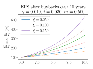
(a) Earnings per share in the presence of buybacks $\frac{E_{n}^{\prime}}{E_{0}}$ (solid lines) and natural earnings per share $\frac{E_{n}}{E_{0}}$ (dashed lines) for a range of values of the natural growth rate $\xi$.

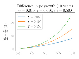
(b) Difference between $\frac{E^{\prime}_{n}}{E_{0}}$ and $\frac{E_{n}}{E_{0}}$ is percentage growth, for each of the values of $\xi_{n}$ in Figure 3.3a.

Figure 3.3: Compounded EPS after a sequence of accretive buybacks

4 Methodology

In the following, we focus on the geometric model for earnings under the effect of a buyback program on real data, examining primarily to what extent accretive buybacks increase earnings per share. Of central interest is what are representative values of $m$ and $\gamma$ in a real setting for which we appeal to the US stock market. We focus on the situation of a sequence of regular buybacks, with the normalised growth in earnings given by (3.6)

$$E_{n}^{\prime}=\left(\frac{(1+\xi)^{c}}{1-\gamma}\right)^{n}\prod_{k=0}^{n}\left(1-m\gamma\left(\frac{1+\imath}{1+\xi}\right)^{ck}\right)E_{0}$$ (4.1)

Estimates of $m=\frac{P}{P^{*}}=\frac{P_{E}}{P_{E}^{*}}$ rely on values of the critical $P_{E}^{*}=\frac{1}{i(1-t_{Tax})}$, which in the case of US stocks we take the 10-year Treasury Constant Maturity bond yield and consider both the prescribed US corporate tax rate and the effective tax rate.

We will use nonlinear least squares to estimate $\xi$ - the natural growth in earnings - from the data. In a statistical setting, the optimisation can be thought of as fitting normally distributed observations, with mean given by 4.1 and constant variance. We therefore minimise

$$(\xi^{\prime},E_{0}):=\arg\min_{(\xi,E_{0})}\sum_{n=0}^{n^{\prime}}\left(R_{n}-E_{n}^{\prime}\right)^{2}$$

where $R_{n}$ is the realised earnings and $E_{n}^{\prime}$ is those under the model in Equation 4.1.

Following methodology similar to [18] we estimate the effective tax rate using the difference between pre-tax and post-tax profits normalised by the pre-tax profits, with the results shown in Figure 4.1.

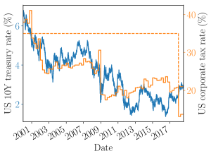
(a) US interest rate and tax rates. (- -) Corporate tax rate (-) Effective tax rate

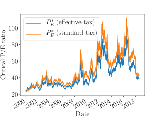
(b) US critical $P_{E}$ with the two tax rates considered

Figure 4.1: Critical P/E, $P_{E}^{*}$, for US market. Interest rate and tax rate data taken from the Federal Reserve.

Figure 4.1a shows both the 10Y bond yield and the two tax rates. Excluding the recent tax reforms we see that the corporate tax has been approximately constant over this period at approximately 40%, whereas the effective tax rate is significantly lower. Importantly, this has an effect on the critical P/E in that by definition it is monotonically decreasing in the tax rate. As such, we plot the critical P/E using both these values in Figure 4.1b where we see that while there is a discrepancy between the two tax rates, the discrepancy is relatively mild. More strikingly, from Figure 4.1b we see an overall positive trend in critical P/E over this period, suggesting that for low-growth companies, in terms of relatively static $P_{E}$ ratios, the result of a buyback is more likely to be accretive and the earnings per share are more likely to be increased after a buyback.

4.1 Apple

We focus on Apple during the period of buybacks initiating in 2013, until the present day, comparing the natural and observed growth rates through the relation of Equation 3.6 after a sequence of buybacks occurring quarterly at regular intervals. The free parameters in the model are $m=\frac{P}{P^{*}}$, the fraction of the critical price paid, $\gamma=\frac{S}{PN}$ the fraction of the market capitalisation spent on buybacks, and $x$ the expected natural growth rate in EPS. We estimate both $m$ and $\gamma$ using the historical data, shown in Figure 4.2, plotting the relevant quantities, value of the buyback (paid quarterly), with $m$ shown to be in the range 0.2 to 0.4 and $\gamma$ shown to vary between 0 and 0.04, with a mean of $0.01$. Taking $m$ and $\gamma$ as the central values of $0.25$ and $0.01$ respectively we compare the historical growth in earnings (shown in $\%$ increase since the start of the period - $1^{st}$ January 2012) for a natural growth rate of $x=0.08$. The results are shown in Figure 4.3b, where we see that over this 5-year period the observed growth in earnings is approximately 188%, however, with a natural estimated growth of only 164%, suggesting that as much of a quarter of the earnings growth over the period ($1-\frac{64}{88}=27\%$ 2s.f.) can be attributable to share repurchases.

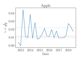
(a) Estimates of $\gamma$ using quarterly buyback data, (- -) median ($\cdot\cdot$) lower and upper 20%-iles.

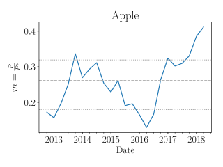
(b) Estimate of ratio of critical $P/E$ using the effective tax rate to calculate the critical $P_{E}^{*}$ (- -) median ($\cdot\cdot$) lower and upper 20%-iles.

Figure 4.2: Apple data used to estimate $m$ and $\gamma$

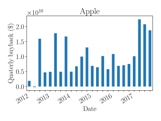
(a) Value of buybacks

(b) Comparison between realised earnings per share $R_{n}$ used to fit the model and earnings per share in the presence of buybacks $E_{n}^{\prime}$ and the natural earnings per share $E_{n}=(1+\xi)^{n}$.

Figure 4.3: Comparison of realised earnings growth and natural growth in the absence of buybacks for Apple shares over a recent 6 year window.

4.2 S&P 500

We consider the natural growth rate for the S&P 500 based on the values of the critical P/E ratio identified above from the quarter ending in $31^{st}$ March 2002 to the quarter ending $29^{th}$ March 2018. In this case, we take values for the S&P 500 P/E ratio, estimating $m$ via $m=\frac{P}{P^{*}}=\frac{P_{E}}{P_{E}^{*}}=\frac{P_{E}}{i(1-t_{tax})}$. Figure 4.4a and plots values of $m$ given by taking the ratio of P/E to the critical P/E, we see that over the financial crisis of 2008/2009 the value for $m$ spikes. This is to a degree as expected owing to the sharp dip in earnings over this time, though the interest rate and tax rate determining $P_{E}^{*}$ is relatively constant. As a result, we take the mean value of $m=0.7$ though note a more refined analysis would consider the variability in natural growth rate as well as the varying values of $m$ through time. We next plot the values of $\gamma$ over this period in Figure 4.4b where we see the average value is $0.007$ (1 s.f.). Based on these values we plot the values of the S&P 500 quarterly earnings with the compounded earnings enhancements from share buybacks overlayed in Figure 4.5. We see that over the last 16 years while the earnings per share accounting for buybacks increased by approximately 364%, the natural growth rate of the S&P 500 was closer to 287%, suggesting that approximately 30% of the growth (1-$\frac{187}{264}$) over this period is as a result of share repurchases of its constituents.

(a) $m=\frac{P}{P^{*}}$ for S&P 500

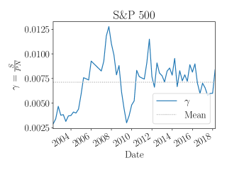
(b) Proportion spent on buybacks of market capitalisation, $\gamma=\frac{S}{NP}$, for S&P 500

Figure 4.4: Values of $m$ and $\gamma$ for S&P 500 from the quarter ending in $31^{st}$ March 2002 to the quarter ending $29^{th}$ March 2018.

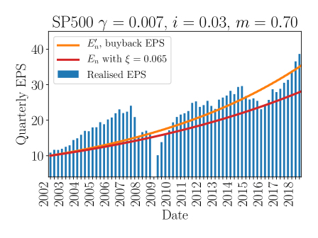
Figure 4.5: Earnings per share in the presence, $E_{n}^{\prime}$, and absence, $E_{n}$, of buybacks for S&P 500 operating earnings per share (quarterly) for the given values of $m$, $\gamma$ and $i$. We compare the growth in earnings implied by the above analysis $E_{n}^{\prime}$ (green) and contrast this with the natural growth rate of $E_{n}$ with $\xi=0.065$ (red).

5 Conclusion

The preceding work provides a quantitative analysis on the mechanical effect of share repurchases on earnings per share. When shares are repurchased for a price below their critical price, the increase in earnings per share can be estimated from a simple cash flow argument. When shares are repurchased as part of a buyback program we are able to estimate the growth in earnings per share that follows as a consequence of the program under both a geometric and arithmetic model for natural earnings growth. We applied the methodology to the US market, analysing the S&P 500 for which we see that buybacks account for around 30% of the earnings growth over the last 16 years and over a quarter of the growth in the case of Apple over the last 5 years.

Appendix A Appendix

A.1 Proof of Proposition 1

Proof.

We consider the earnings at time $T$ after a buyback at time $t$. If we assume that no event affects the number of shares in the period between $t$ and $T$ we have that, $N_{t}=N_{T}$ and in the case of a buyback $N_{t}^{\prime}=N_{t}-\frac{S_{t}}{P_{t}}$. As such we have the earnings at time $T$ given by

$$E_{T}^{\prime} =\frac{\alpha\left(O_{T}+(C_{t}-S_{t})iI_{t,T}\right)}{N_{t}^{\prime}}$$

$$=\frac{\alpha\left(O_{T}+(C_{t}-S_{t})iI_{t,T}\right)}{N_{t}-\frac{S_{t}}{P_{t}}}$$

$$=\frac{\alpha}{1-\frac{S_{t}}{P_{t}N_{t}}}\left(\frac{O_{T}+C_{t}iI_{t,T}}{N_{t}}-\frac{S_{t}iI_{t,T}}{N_{t}}\right)$$

$$=\frac{1}{1-\gamma_{t}}\left(E_{T}-\frac{S_{t}i\alpha}{N_{t}}I_{t,T}\right)$$

$$=\frac{1}{1-\gamma_{t}}\left(E_{T}-m_{t}\gamma_{t}I_{t,T}E_{t}\right)$$ (A.1)

and using the definition of the critical P/E ratio $P_{E}^{*}(t):=\frac{P_{t}^{*}}{E_{t}}=\frac{1}{\alpha i}$. Provided $E_{T}\geq m_{t}\gamma_{t}I_{t,T}E_{t}$ (i.e. that $m_{t}\gamma_{t}\leq 1$ in the presence of low interest rates and accretive buybacks) we have that

$$E_{T}^{\prime} =\frac{E_{T}-m_{t}I_{t,T}E_{t}\gamma_{t}}{1-\gamma_{t}}$$

$$=E_{T}+(E_{T}-m_{t}I_{t,T}E_{t})\sum_{n=1}^{\infty}\gamma_{t}^{n}$$

$$=E_{T}+(E_{T}-m_{t}I_{t,T}E_{t})\gamma_{t}+\mathcal{O}(\gamma_{t}^{2})$$

$$\geq E_{T}+\left(E_{T}-m_{t}I_{t,T}E_{t}\right)\gamma_{t}$$

where the remainder is positive by inspection. The series expansion can be derived through the identity

$$\frac{a-bx}{1-x} =\lim_{M\rightarrow\infty}(a-bx)\sum_{n=0}^{M}x^{n}$$

$$=\lim_{M\rightarrow\infty}(a\sum_{n=0}^{M}x^{n}-b\sum_{n=1}^{M+1}x^{n})$$

$$=\lim_{M\rightarrow\infty}(a+(a-b)\sum_{n=0}^{M}x^{n}-bx^{M+1})$$

$$=a+(a-b)\sum_{n=0}^{\infty}x^{n}$$

for $|x|\leq 1$. ∎

A.2 Arithmetic earnings growth

In the following we consider the arithmetic growth rate $E(t+\Delta t)-E_{t}=\Delta x$. We model both the natural earnings $E_{t}$ and the accumulated interest rate $I_{t,T}$ as stochastic processes. For the purposes of simplicity we consider buybacks occuring at regular times $\{0,\Delta t,2\Delta t,3\Delta t,...\}$ so that we are able to consider only discrete time processes. Letting $\mathds{E}[X]$ denote the expectation of a random variable $X$ we assume that $E_{t}$ follows some random walk with constant expected mean, i.e. that

$$\bar{x}:=\mathds{E}[E(t+\Delta t)-E_{t}|E_{t}]$$

is constant for all $t$. We additionally assume the expected interest rate over a single $\Delta t$ period is approximately constant, i.e. $\mathds{E}\left[I(t,t+\Delta t)\right]=(1+\imath)^{\Delta t}$ , so from (A.1) we have that the expected earnings after a buyback occuring at time $t$ a unit of time $\Delta t$ later is

$$\mathds{E}\left[E^{\prime}(t+\Delta t)\right] =\mathds{E}\left[\frac{E(t+\Delta t)-m_{t}I(t,t+\Delta t)E_{t}}{1-\gamma_{t}}\right]$$

$$=\mathds{E}\left[\mathds{E}\left[\frac{\Delta x+E_{t}-m_{t}I(t,t+\Delta t)E_{t}}{1-\gamma_{t}}|\{E_{t}\}\right]\right]$$

$$=\mathds{E}\left[\mathds{E}\left[\frac{\Delta x}{1-\gamma_{t}}|\{E_{t}\}\right]+\mathds{E}\left[\frac{1-m_{t}I(t,t+\Delta t)}{1-\gamma_{t}}|\{E_{t}\}\right]E_{t}\right]$$

$$=\left(\frac{1-m_{t}(1+\imath)^{\Delta t}}{1-\gamma_{t}}\right)\mathds{E}\left[E_{t}\right]+\frac{\bar{x}}{1-\gamma_{t}}$$

Such a result allows us to consider a sequence of buybacks occuring at regular intervals, every $\Delta t$ time increments. In particular we have that $\mathds{E}\left[E^{\prime}(t+\Delta t)\right]=a\mathds{E}\left[E_{t}\right]+b$ for constants $a$ and $b$ that do not depend on earnings. Repeated application of this identity leads to

$$\mathds{E}\left[E(k\Delta t)\right] =a^{k}E_{0}+b\frac{1-a^{k}}{1-a}$$

$$=\left(\frac{1-(1+\imath)m\gamma}{1-\gamma}\right)^{k}E_{0}+\frac{\bar{x}}{1-\gamma}\left(\frac{1-\left(\frac{1-(1+\imath)m\gamma}{1-\gamma}\right)^{k}}{1-\left(\frac{1-(1+\imath)m\gamma}{1-\gamma}\right)}\right)$$

making the simplifying assumption that $\gamma_{t}=\gamma$, i.e. the fraction spent on buybacks at any time instance is approximately constant for all $t$. As a result we see that even when a company’s expected growth rate is close to 0 in the absence of a repurchase program we have that

$$\mathds{E}\left[E(k\Delta t)\right]=\left(\frac{1-(1+\imath)m\gamma}{1-\gamma}\right)^{k}E_{0}$$

suggesting even under an arithmetic model for earnings growth, the affect on earnings of a buyback program can not only appear to inflate expected earning but do so also at a geometric rate. Furthermore, we see if in addition interest rates are low then

$$\mathds{E}\left[E(k\Delta t)\right]\approx\left(\frac{1-m\gamma}{1-\gamma}\right)^{k}E_{0}$$

which is precisely the $k^{th}$ power of the earnings enhancement occuring instantaneously at $k=0$, suggesting that in such a regime we may be able to approximate the earnings enhancement through time by simply taking the power of the instantaneous earnings enhancement. Indeed, it suggests even though a company’s earnings may not intrinsically be growing, if it is able to buyback its shares cheaply it is able to appear to grow geometrically.

A.3 Stochastic earnings enhancement

We here introduce a simple model for uncertainty of the above where we make the simplifying assumption that the earnings per share cannot be negative. In this case we are able to instead treat $i(t)\in\mathds{R}^{+}$ and $x(t)\in\mathds{R}^{+}$ as discrete time stochastic processes defined on a probability space $(\Omega,\mathcal{F},\mathds{P})$, with $\Omega=\mathbb{N}\times\mathds{R}^{+}$ and $\mathcal{F}$ the generated $\sigma$-algebra. We see in this case that the earnings per share with and without a buyback are now stochastic processes. Following the reasoning as before, we are able to construct the following process quantifying the relative change between the earnings with and without a buyback as

$$G(t):=\frac{E_{t}^{\prime}}{E_{t}}=\frac{1}{1-\gamma}\left(1-m\gamma\frac{i(t)}{x(t)}\right)$$

For the purposes of tractability, if we let $i(t)=\prod_{p=1}^{t}(1+\epsilon_{p})$ and $x(t)=\prod_{p=1}^{t}(1+\delta_{p})$ where $1+\epsilon_{p}\stackrel{{\scriptstyle i.i.d}}{{\sim}}\ln\mathcal{N}(\mu_{i},\sigma_{i}^{2})$ and $1+\delta_{p}\stackrel{{\scriptstyle i.i.d}}{{\sim}}\ln\mathcal{N}(\mu_{x},\sigma_{x}^{2})$ (we assume that both are independent of each other) then we recover the following exact expressions for the mean of the increase in earnings as

$$\mathds{E}\left[G(t)\right] =\frac{1}{1-\gamma}\left(1-m\gamma\mathds{E}\left[\frac{i(t)}{x(t)}\right]\right)$$

$$=\frac{1}{1-\gamma}\left(1-m\gamma\mathds{E}\left[\prod_{p=1}^{t}\frac{1+\epsilon_{p}}{1+\delta_{p}}\right]\right)$$

$$=\frac{1}{1-\gamma}\left(1-m\gamma\exp\left(t\left(\mu_{i}-\mu_{x}+\frac{\sigma_{i}^{2}+\sigma_{x}^{2}}{2}\right)\right)\right)$$

using standard properties of the lognormal distribution. Such a result suggests that as either the interest rate or growth rate volatility increases the expected increase is dampened through time. Finally, we see that the standard deviation of the process at time $t$ is expressed as

$$\sigma(t) :=\sqrt{\mathds{V}\left[G(t)\right]}=\frac{m\gamma}{1-\gamma}\exp\left(\mu_{i}-\mu_{x}+\frac{\sigma_{i}^{2}+\sigma_{x}^{2}}{4}\right)\sqrt{\exp\left(\frac{\sigma_{i}^{2}+\sigma_{x}^{2}}{2}\right)-1}$$

where we see a monotone increase with $\gamma$ (noting that $\gamma\in[0,1]$), $\mu_{i}-\mu_{x}$, $\sigma_{i}^{2}$ or $\sigma_{x}^{2}$ .

References

- [1] Daniel A Bens, Venky Nagar, Douglas J Skinner, and MH Franco Wong. Employee stock options, eps dilution, and stock repurchases. Journal of Accounting and Economics, 36(1-3):51–90, 2003.
- [2] Richard Dobbs and Werner Rehmn. The value of share buybacks. McKinsey Quarterly, 2005.
- [3] Jonathan Ford. Boeing and the siren call of share buybacks. The Financial Times, 2019.
- [4] Justin Fox. The big and possibly dumb buyback boom. Bloomberg Opinion, 2018.
- [5] Nico Grant and Ian King. Big tech’s big tax ruse: Industry splurges on buybacks. Bloomberg, 2019.
- [6] Joseph Gruber and Steven Kamin. Corporate buybacks and capital investment: An international perspective. IFDP notes, 2017.
- [7] Gustavo Grullon and David L Ikenberry. What do we know about stock repurchases? Journal of Applied Corporate Finance, 13(1):31–51, 2000.
- [8] Gustavo Grullon and Roni Michaely. The information content of share repurchase programs. The Journal of Finance, 59(2):651–680, 2004.
- [9] Richard Henderson. Fall in share buybacks poses threat to us stocks. The Financial Times, 2019.
- [10] Richard Henderson. Share buybacks on course for record year. The Financial Times, 2019.
- [11] Paul Hribar, Nicole Thorne Jenkins, and W Bruce Johnson. Stock repurchases as an earnings management device. Journal of Accounting and Economics, 41(1-2):3–27, 2006.
- [12] Murali Jagannathan, Clifford P Stephens, and Michael S Weisbach. Financial flexibility and the choice between dividends and stock repurchases. Journal of financial Economics, 57(3):355–384, 2000.
- [13] Justin Pettit. Is a share buyback right for your company? 2001.
- [14] Matthew Rocco. Stock buybacks ramp up while investors turn to etfs ? bofa. The Financial Times, 2019.
- [15] Matthew Rocco. Us corporate cash pile shrinks as spending climbs after tax cuts. The Financial Times, 2019.
- [16] Richard Waters. Google parent alphabet overtakes apple to become new king of cash. The Financial Times, 2019.
- [17] Richard Waters and Andrew Edgecliffe-Johnson. Five us tech giants spend combined $115bn on buying back stock. The Financial Times, 2018.
- [18] Edward Yardeni. Us economic indicators: Corporate taxes. Technical report, 2018.