Abstract

Recognising and locating image patches or sets of image features is an important task underlying much work in computer vision. Traditionally this has been accomplished using template matching. However, template matching is notoriously brittle in the face of changes in appearance caused by, for example, variations in viewpoint, partial occlusion, and non-rigid deformations. This article tests a method of template matching that is more tolerant to such changes in appearance and that can, therefore, more accurately identify image patches. In traditional template matching the comparison between a template and the image is independent of the other templates. In contrast, the method advocated here takes into account the evidence provided by the image for the template at each location and the full range of alternative explanations represented by the same template at other locations and by other templates. Specifically, the proposed method of template matching is performed using a form of probabilistic inference known as “explaining away”. The algorithm used to implement explaining away has previously been used to simulate several neurobiological mechanisms, and been applied to image contour detection and pattern recognition tasks. Here is is applied for the first time to image patch matching, and is shown to produce superior results in comparison to the current state-of-the-art methods.

Keywords:

Template matching; Feature detection; Image matching; Image registration; Correspondence Problem; Multi-view Vision

1 Introduction

Recognising that one part of an image contains a particular object, image structure or set of local image features is a fundamental sub-problem in many image processing and computer vision algorithms. For example, it can be used to perform object detection or recognition by identifying parts belonging to an object category (Lowe,, 1999; Leibe et al.,, 2008; Csurka et al.,, 2004), or for navigation by identifying and locating landmarks in a scene (Özuysal et al.,, 2010; Se et al.,, 2005), or for image mosaicing/stitching by identifying corresponding locations in multiple images (Szeliski,, 2006; Brown and Lowe,, 2007). Similarly, extracting a distinctive image structure in one image and then recognising and locating that same feature in another image of the same scene taken from a different viewpoint, or at a different time, is essential to solving the stereo and video correspondence problems, and hence, for calculating depth or motion, and for performing image registration and tracking (Lucas and Kanade,, 1981; Brown et al.,, 2003; Gall et al.,, 2011; Zitová and Flusser,, 2003). Finally, locating specific image features is fundamental to tasks such as edge detection (Canny,, 1986). In this latter case the image structure being searched for is usually defined mathematically (e.g., a Gaussian derivative for locating intensity discontinuities), whereas for solving image stitching and correspondence problems the image structure being searched for is extracted from another image, and in the case of object or landmark recognition the target image features may have been learnt from a set of training images.

Image patch recognition has traditionally been accomplished using template matching (Ma et al.,, 2009; Wei and Lai,, 2008; Goshtasby et al.,, 1984; Barnea and Silverman,, 1972). In this case the image structure being searched for is represented as an array of pixel intensity values, and these values are compared with the pixel intensities around every location in the query image. There are many different metrics that can be used to quantify how well the template matches each location in an image; such as the sum of absolute differences (SAD), the normalised cross-correlation (NCC), the sum of squared differences (SSD) or the zero-mean normalised cross correlation (ZNCC). For any metric it is necessary to define a criteria that needs to be met for a patch of image to be considered a match to the template. For correspondence problems, it is often assumed that the image structure being searched-for will match exactly one location in the query image. The location with the highest similarity to the template is thus considered to be the matching location. However, additional criteria, such as the ratio of the two highest similarity values, may be used to reject some such putative matches. In other tasks, the image structure being searched for may occur zero, one or multiple times in the query image. In this case it is necessary to define a global threshold to distinguish those image locations where the template matches the query image from those locations where it does not. It is also typically the case that for a patch of image to be considered a match to the template it must be more similar to the template than its immediate neighbours. Hence, locations where the template is considered to match the image are ones where the similarity metric is a local maximum and exceeds a global threshold.

With traditional template matching, because the metric for assessing the similarity of the template and a patch of image compares intensity values, the result can be effected by changes in illumination. This issue can be resolved by using a metric such as ZNCC which subtracts the mean intensity from the template and from the image patch it is being compared to. This results in a comparison of the relative intensity values and produces a similarity measure that is tolerant to differences in lighting conditions between the query image and the template.

Another issue is that the metric for assessing the similarity of a template to a patch of image is based on pixel-wise comparisons of intensity values. The results will therefore be effected if the pixels being compared do not correspond to the same part of the target image structure. This problem can arise due to differences in the appearance of the image structure between the query image and the template, caused by variations in viewpoint, partial occlusion, and non-rigid deformations. To be able to recognise image features despite such changes in appearance one approach is to use multiple templates that represent the searched-for image patch across the range of expected changes in appearance. However, even small differences in scale, orientation, aspect ratio, etc. can result in sufficient mis-alignment at the pixel-level that a low value of similarity is calculated by the similarity metric for all transformations of the template when compared to the correct location in the query image. Hence, to allow tolerance to viewpoint, even when using multiple templates for each image feature, it is necessary to use a low threshold to avoid excluding true matches. However, given the large number of comparisons that are being made between all templates and all image locations, a low threshold will inevitably lead to false-positives. There is thus an irreconcilable need both for a high threshold to avoid false matches and for a low threshold in order not to exclude true matches in situations where the template is not perfectly aligned with the image. These problems have lead to template matching being abandoned in favour of alternative methods (see sect. 2) for most tasks except for low-level ones such as edge detection.

This article shows that the performance of template matching can be significantly improved by requiring templates to compete with each other to match the image. The particular type of competition used in the proposed method, called Divisive Input Modulation (DIM Spratling et al.,, 2009; Spratling,, 2017), implements a form of probabilistic inference known as “explaining away” (Kersten et al.,, 2004; Lochmann and Deneve,, 2011). This means that the similarity between a template and a patch of image takes into account not only the similarity in the pixel intensity values at corresponding locations in the template and the patch, but also the range of alternative explanations for the patch intensity values represented by the same template at other locations and by other templates. If the similarity between a template and each image location is represented by an array, then this array is dense for traditional template matching. In contrast, due to the competition employed by the proposed method, the array of similarity values is very sparse. Those locations that match a template can therefore be more readily identified and there is typically a much larger range of threshold values that separate true matches from false matches.

2 Related Work

Given the issues with template matching discussed above, many alternative methods for locating image features have been developed. Typically, these alternative methods change the way the template and image patch are represented, so that the comparison is performed in a different feature-space, or change the computation that is used to perform the comparison, or use a combination of both.

One alternative is to employ a classifier in place of the comparison of corresponding pixel intensity values used in traditional template matching. For example, random trees and random ferns can be trained using image patches seen from multiple viewpoints in order to robustly recognise those image features when they appear around keypoints extracted from a new image (Gall et al.,, 2011; Özuysal et al.,, 2010; Lepetit and Fua,, 2006). Sliding-window based methods apply the classifier, sequentially, to all regions within the image (Dalal and Triggs,, 2005; Lampert et al.,, 2008), while region-based methods select a sub-set of image patches for presentation to the classifier (Girshick et al.,, 2016; Gu et al.,, 2009; Uijlings et al.,, 2013). In each case, the classifier provides robustness to changes in appearance due to, for example, viewpoint or within-class variation. Further tolerance to appearance can be achieved by using windows with different sizes and aspect ratios. A classifier in the form of a deep neural network can also be used to directly assess the similarity between two image patches (Zagoruyko and Komodakis,, 2015, 2017).

Instead of being used to perform the comparison between a template and an image patch, a deep neural network can also be used to extract features from the image and template for comparison (i.e., a deep neural network can be used to change the feature-space, rather than change the similarity computation). For example, Kim et al., (2017) used a convolutional neural network (CNN) to represent both the template and the image in a new feature-space, the comparison was then carried out using NCC.

Histogram matching is another method that changes the feature-space. Histogram matching compares the colour histograms of the template and image patch, and hence, disregards all spatial information (Comaniciu et al.,, 2000). This will introduce tolerance to differences in appearance, but also reduces the ability to discriminate between spatially distinct features. Co-occurrence based template matching (CoTM) calculates the cost of matching a template to an image patch as inversely proportional to the probability of the corresponding pixel values co-occurring in the image (Kat et al.,, 2018). This can be achieved by mapping the points in the image and template to a new feature-spaced defined by the co-occurrence statistics. However, this method does not work well for grayscale images or images containing repeating texture, and is not tolerant to differences in illumination (Kat et al.,, 2018).

Another approach to is to perform comparisons on more distinctive image features than image intensity values. For example, the scale-invariant feature transform (SIFT) generates an image descriptor that is invariant to illumination, orientation, and scale and partially invariant to affine distortion (Lowe,, 1999, 2004). Methods to allow SIFT descriptors to be matched across images with invariance to affine transformations have also been developed (Morel and Yu,, 2009; Dong and Soatto,, 2015). Many alternative feature descriptors have also been proposed, such as SURF (Bay et al.,, 2006), BRIEF (Calonder et al.,, 2010), ORB (Rublee et al.,, 2011), GLOH (Mikolajczyk and Schmid,, 2005), DAISY (Tola et al.,, 2008), and BINK (Saleiro et al.,, 2017). However, experiments comparing the performance of different image descriptors for finding matching locations between images of the same scene suggest that SIFT remains one of the most accurate methods (Balntas et al.,, 2018; Mikolajczyk and Schmid,, 2005; Wu et al., 2013a, ; Tareen and Saleem,, 2018; Balntas et al., 2017b, ; Mukherjee et al.,, 2015; Khan et al.,, 2015). It is also possible to learn image descriptors, and this approach can improve performance beyond that of hand-crafted descriptors (Trzcinski et al.,, 2012; Brown et al.,, 2011; Simonyan et al.,, 2014; Schönberger et al.,, 2017). Recently, learning image descriptors using deep neural networks has become a popular approach (Kwang et al.,, 2016; Simo-Serra et al.,, 2015; Balntas et al.,, 2018; Balntas et al., 2017a, ; Balntas et al.,, 2016; Zagoruyko and Komodakis,, 2015, 2017; Mitra et al.,, 2017).

Another alternative to traditional template matching, that can perform image patch matching with tolerance to changes in appearance, is image alignment. In these methods the aim is to find the affine transformation that will align a template with the image (Lucas and Kanade,, 1981; Zhang and Akashi,, 2015; Korman et al.,, 2013). For example, FAsT-Match is a relatively recent algorithm of this type that measures the similarity between a template and an image patch by first searching for the 2D affine transformation that maximises the pixel-wise similarity (Korman et al.,, 2013). However, it is limited to working with grayscale images and the large search-space of possible affine transformations makes this algorithm slow. A more recent variation on this algorithm, OATM (Korman et al.,, 2018), has increased speed but remains both slower and less accurate than another approach, DDIS, which is discussed in the following paragraph.

Another approach is to define alternative metrics for comparing the template with the image that allow for mis-alignment between the pixels in the template and the corresponding pixels in the image, rather than rigidly comparing pixels at corresponding locations in the template and the image. Typically, these metrics are based on measuring the distance between points in the template and the best matching points in the image (Talmi et al.,, 2017; Dekel et al.,, 2015; Oron et al.,, 2018). For example, the Best-Buddies Similarity (BBS) metric (Dekel et al.,, 2015; Oron et al.,, 2018) is computed by counting the proportion of sub-regions in the template and the image patch that are “best-buddies”. For each sub-region in the template the most similar sub-region (in terms of position and colour) is found in the image patch. For each sub-region in the image patch the most similar sub-region in the template is calculated in the same way. A pair of sub-regions are best-buddies if they are most similar to each other. Sub-regions can be best-buddies even if they are not at corresponding locations in the template and the image patch, and this thus provides tolerance to differences in appearance between the template and the patch. Deformable diversity similarity (DDIS) is similar to BBS, but it differs in the way it deals with spatial deformations, and the criteria used for determining if sub-regions in the image patch and template match (Talmi et al.,, 2017). Specifically, for every sub-region of the image patch the most similar sub-region (in terms of colour only) is found in the template. The contribution of each such match to the overall similarity is inversely weighted by the number of other sub-regions that have been matched to the same location in the template, and by the spatial distance between the matched sub-regions in the image patch and the template. DDIS produces the current state-of-the-art performance when applied to template matching in colour-feature space on standard benchmarks (Talmi et al.,, 2017; Kat et al.,, 2018).

This article proposes another alternative method of image patch matching. Like traditional template matching, the proposed method compares pixel-intensity values in the template with those at corresponding locations in the image patch. However, in contrast to traditional template matching the similarity between any one template and the image patch is not independent of the other templates. Instead, the templates compete with each other to be matched to the image patch. This article describes empirical tests of this new approach to template matching that demonstrate that it provides tolerance to differences in appearance between the template and the same image feature in the query image. This results in more accurate identification of features in an image compared to both traditional template matching and recent state-of-the-art alternatives to template matching (Talmi et al.,, 2017; Dekel et al.,, 2015; Oron et al.,, 2018; Kat et al.,, 2018; Kim et al.,, 2017; Zagoruyko and Komodakis,, 2015, 2017).

3 Methods

3.1 Image Pre-processing and Template Definition

Image features are better distinguished using relative intensity (or contrast) rather than absolute intensity. For this reason, ZNCC is a sensible choice of similarity metric for template matching. ZNCC subtracts the mean intensity from the template and from the image patch it is being compared to. Subtracting the mean intensity will obviously result in positive and negative relative intensity values. However, non-negative inputs are required by the mechanism that is used in this article to implement template matching using explaining away (see sect. 3.2). Hence, to allow the proposed method to process relative intensity values the input image was pre-processed as follows.

A grayscale input image $I$ was convolved with a 2D circular-symmetric Gaussian mask $g$ with standard deviation equal to $\sigma$ pixels, such that: $\bar{I}=I\ast g$. $\bar{I}$ is an estimate of the local mean intensity across the image. To avoid a poor estimate of $\bar{I}$ near the borders, the image was first padded on all sides with intensity values that were mirror reflections of the image pixel values near the borders of $I$. The width of the padding was equal to the width of the template on the left and right borders, and equal to the height of the template on the the top and bottom borders. Once calculated $\bar{I}$ could be cropped to be the same size as the original input image. However, to avoid edge-effects when template matching, $\bar{I}$ was left padded and all the arrays the same size as $\bar{I}$ (i.e., $\mathbf{X}$, $\mathbf{R}$, $\mathbf{E}$, and $\mathbf{Y}$ see sect. 3.2) were cropped to be the same size as the original image once the template matching method had been applied. The relative intensity can be approximated as $\mathbf{X}=2(I-\bar{I})$. To produce only non-negative input to the proposed method, the positive and rectified negative values of $\mathbf{X}$ were separated into two images $\mathbf{X}_{1}$ and $\mathbf{X}_{2}$. Hence, for grayscale images the input to the model was two arrays representing increases and decreases in local contrast. For colour images each colour channel was pre-processed in the same way, resulting in six input arrays ($\mathbf{X}_{1}\dots\mathbf{X}_{6}$) representing the increases and decreases about the average value in each colour channel.

For grayscale images a template consists of two arrays of values ($\mathbf{w}_{j1}$ and $\mathbf{w}_{j2}$) which are compared to $\mathbf{X}_{1}$ and $\mathbf{X}_{2}$. Similarly for a colour image a template consists of six arrays of values ($\mathbf{w}_{j1}\dots\mathbf{w}_{j6}$). These arrays can be produced by performing the pre-processing operation described in the previous paragraph on a standard template of intensity values (which could have been defined mathematically, have been learnt, or have been a patch extracted from an image). Alternatively, the templates can be created by extracting regions from images that have been processed as described in the preceding paragraph. This latter method was used in all the experiments reported in this article. The value of $\sigma$ was set equal to half of the template width or height, whichever was the smaller of the two dimensions.

3.2 Template Matching

The proposed method of template matching was implemented using the Divisive Input Modulation (DIM) algorithm (Spratling et al.,, 2009). This algorithm has been used previously to simulate neurophysiological (Spratling,, 2011) and psychological data (Spratling, 2016b, ) and applied to tasks in robotics (Muhammad and Spratling,, 2015), pattern recognition (Spratling,, 2014) and computer vision (Spratling,, 2013, 2017). The DIM algorithm is described in these previous publications, but this description is repeated here for the convenience of the reader. DIM was implemented using the following equations:

$$\mathbf{R}_{i}=\sum_{j=1}^{p}\left(\mathbf{v}_{ji}\ast\mathbf{Y}_{j}\right)$$ (1)

$$\mathbf{E}_{i}=\mathbf{X}_{i}\oslash\left[\mathbf{R}_{i}\right]_{\epsilon_{2}}$$ (2)

$$\mathbf{Y}_{j}\leftarrow\left[\mathbf{Y}_{j}\right]_{\epsilon_{1}}\odot\sum_{i=1}^{k}\left(\mathbf{w}_{ji}\star\mathbf{E}_{i}\right)$$ (3)

Where $i$ is the index over the number of input channels (the maximum index $k$ is two for grayscale images and six for colour images), $j$ is an index over the number, $p$, of different templates being compared to the image; $\mathbf{X}_{i}$ is a 2-dimensional array generated from the original image by the pre-processing method described in sect. 3.1; $\mathbf{R}_{i}$ is a 2-dimensional array representing a reconstruction of $\mathbf{X}_{i}$; $\mathbf{E}_{i}$ is a 2-dimensional array representing the discrepancy (or residual error) between $\mathbf{X}_{i}$ and $\mathbf{R}_{i}$; $\mathbf{Y}_{j}$ is a 2-dimensional array that represent the similarity between template $j$ and the image at each pixel; $\mathbf{w}_{ji}$ is a 2-dimensional array representing channel $i$ of template $j$ defined as described in sect. 3.1; $\mathbf{v}_{ji}$ is a 2-dimensional array also representing template values ($\mathbf{v}_{ji}$ and $\mathbf{w}_{ji}$ differ only in the way they are normalised, as described below); $\left[v\right]_{\epsilon}=\texttt{max}(\epsilon,v)$; $\epsilon_{1}$ and $\epsilon_{2}$ are parameters; $\oslash$ and $\odot$ indicate element-wise division and multiplication respectively; $\star$ represents cross-correlation; and $\ast$ represents convolution (which is equivalent to cross-correlation with the kernel rotated $180^{o}$).

DIM attempts to find a sparse set of elementary components that when combined together reconstruct the input with minimum error (Spratling,, 2014). For the current application, the elementary components are the templates reproduced at every location in the image, and all templates at all locations can be thought of as a “dictionary” or “codebook” that can be used to reconstruct many different inputs. The activation dynamics, described by eq. 1, 2 and 3, perform gradient descent on the residual error in order to find values of $\mathbf{Y}$ that accurately reconstruct the current input (Achler,, 2014; Spratling et al.,, 2009; Spratling,, 2012). Specifically, the equations operate to find values for $\mathbf{Y}$ that minimise the Kullback-Leibler divergence between the input ($\mathbf{X}$) and the reconstruction of the input ($\mathbf{R}$) (Spratling et al.,, 2009; Solbakken and Junge,, 2011). The activation dynamics thus result in the DIM algorithm selecting a subset of dictionary elements that best explain the input. The strength of an element in $\mathbf{Y}$ reflects the strength with which the corresponding dictionary entry (i.e., template) is required to be present in order to accurately reconstruct the input at that location.

Each element in the similarity array $\mathbf{Y}$ can be considered to represents a hypothesis about the image features present in the image, and the input $\mathbf{X}$ represents sensory evidence for these different hypotheses. Each similarity value is proportional to the belief in the hypothesis represented, i.e., the belief that the image features represented by that template are present at that location in the image. If a template and a patch of image have strong similarity this will inhibit the inputs being used to calculate the similarity of the same template at nearby locations (ones where the templates overlap spatially), and will also inhibit the inputs being used to calculate the similarity of other templates at the same and nearby locations. Thus, hypotheses that are best supported by the sensory evidence inhibit other competing hypotheses from receiving input from the same evidence. Informally we can imagine that overlapping templates inhibit each other’s inputs. This generates a form of competition between templates, such that each one effectively tries to block other templates from responding to the pixel intensity values which it represents (Spratling et al.,, 2009; Spratling,, 2012). This competition between the templates performs explaining away (Kersten et al.,, 2004; Lochmann and Deneve,, 2011; Spratling,, 2012; Spratling et al.,, 2009). If a template wins the competition to respond to (i.e., have a high similarity to) a particular pattern of inputs, then it inhibits other templates from responding to those same inputs. Hence, if one template explains part of the evidence (i.e., a patch of image), then support from this evidence for alternative hypotheses (i.e., templates) is reduced, or explained away.

The sum of the values in each template, $\mathbf{w}_{j}$, was normalised to sum to one. The values of $\mathbf{v}_{j}$ were made equal to the corresponding values of $\mathbf{w}_{j}$, except they were normalised to have a maximum value of one. The cross-correlation operator used in equation 3 calculates the similarity, $\mathbf{Y}$, for the same set of templates, $\mathbf{w}$, at every pixel location in the image. The convolution operation used in equation 1 calculates the reconstructions, $\mathbf{R}$, for the same set of templates, $\mathbf{v}$, at every pixel location in the image. The rotation of the kernel performed by convolution ensures that each channel of the reconstruction $\mathbf{R}_{i}$ can be compared pixel-wise to the actual input $\mathbf{X}_{i}$.

For all the experiments described in this paper (except those exploring parameter sensitivity reported in sect. 4.4) $\epsilon_{1}$ and $\epsilon_{2}$ were given the values $\frac{\epsilon_{2}}{max\left(\sum_{j}v_{ji}\right)}$ and $1\times 10^{-2}$ respectively. Parameter $\epsilon_{1}$ allows elements of $\mathbf{Y}$ that are equal to zero, to subsequently become non-zero. Parameter $\epsilon_{2}$ prevents division-by-zero errors and determines the minimum strength that an input is required to have in order to effect the values of $\mathbf{Y}$. As in all previous work with DIM, these parameters have been given small values compared to typical values of $\mathbf{Y}$ and $\mathbf{R}$, such that they have negligible effects on the steady-state values of $\mathbf{R}$, $\mathbf{E}$ and $\mathbf{Y}$. To determine these steady-state values, all elements of $\mathbf{Y}$ were initially set to zero, and eq. 1 to 3 were then iteratively updated with the new values of $\mathbf{Y}$ calculated by eq. 3 substituted into eq. 1 and 3. This iterative process was terminated after 10 iterations for the experiments reported in sect. 4.1 and 4.2 (where the number of templates varied between 1 and 31) and 20 iterations for the experiments reported in sect. 4.3 (where 70 templates were used). It is necessary to increase the number of iterations used as the number of templates increases as the competition between the templates takes longer to be resolved. However, for a fixed number of templates the results were not particularly sensitive to the exact number of iterations used (see sect. 4.4). The values in array $\mathbf{Y}_{j}$ produced at the end of the iterative process were used as a measure of the similarity between template $j$ and the input image over all spatial locations.

3.3 Post-Processing

While the similarity array $\mathbf{Y}_{j}$ for template $j$ is sparse, it is not always the case that the best matching location is represented by a single element with a large value. Often the best matching location will be represented by a small population of neighbouring elements with high values. The size of this population is usually proportional to the size of the template. To sum the similarity values within neighbourhoods the similarity array produced by each template was convolved with a binary-valued kernel that contained ones within an elliptically shaped region with width and height equal to $\lambda$ times the width and height of the template. The size of the region over which values were summed was restricted to be at least one pixel, so that a small $\lambda$ and/or a small template size did not result in a summation of zero pixels, but would instead result in an output that was the same as the original $\mathbf{Y}_{j}$. A value of $\lambda=0.025$ was used in all experiments unless otherwise stated. However, the results were not particularly sensitive to the value of $\lambda$ and similar results were obtained with a range of different values (see sect. 4.4).

3.4 Implementation

Open-source software, written in MATLAB, which performs all the experiments described in this article is available for download from: http://www.corinet.org/mike/Code/dim_patchmatching.zip. This code compares the performance of DIM to that of several other methods. Firstly, the BBS method (Dekel et al.,, 2015; Oron et al.,, 2018) which was implemented using the code supplied by the authors of BBS. Secondly, the DDIS algorithm (Talmi et al.,, 2017) which was implemented using the code provided by the authors of DDIS. Finally, traditional template matching using ZNCC as the similarity metric which was implemented using the MATLAB command normxcorr2. This command is part of the MATLAB Image Processing Toolbox.

As described in sect. 3.1, the proposed method can be applied to grayscale or colour images. For colour images, the best results were found using images in CIELab colour space. For a fair comparison, all other algorithms were also applied to colour images. Specifically, BBS was applied to RGB images (as in Dekel et al.,, 2015), DDIS was also applied to RGB images (as in Talmi et al.,, 2017). ZNCC was applied to HSV images as this was found to produce better results than either RGB or CIELab. To apply ZNCC to colour images the similarity values were calculated using ZNCC independently for each colour channel, and then these values were summed to produce the final measure of similarity.

4 Results

4.1 Correspondence using the Best Buddies Similarity Benchmark

This section describes an experiment in which a template is extracted from one image and is used to find the best matching location in a second image of the same scene. Specifically, each image pair consists of two frames from a video. Within each image the bounding-box of a target object has been defined manually. Between the images in each pair, the image patch corresponding to the target changes in appearance due to variations in viewpoint and lighting conditions, changes in the pose of the target, partial occlusions, non-rigid deformations of the target, and due to changes in the surrounding context and background. In total there are 105 image pairs taken from 35 colour videos that have previously been used as an object tracking benchmark (Wu et al., 2013b, ). This dataset was originally prepared to evaluate the performance of the BBS template matching algorithm (Dekel et al.,, 2015). Experimental procedures equivalent to those used in Dekel et al., (2015) have also been used here. Specifically, the bounding-box in the first image of each pair was used to define a template. The template matching method was then used to calculate the similarity between this template and every location in the second image of the same pair. The single location which had the highest similarity was used as the predicted location of the target. A bounding-box, the same size as the one in the first image, was defined around this predicted location and the overlap between this and the bounding-box provided in the ground-truth data was determined, and used as a measure of the accuracy of the template matching. This bounding box overlap was calculated, in the standard way, as the intersection over union (IoU) of the two bounding boxes.

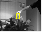
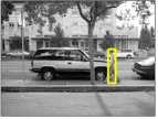
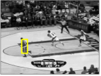
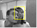
(1 tpl)

(1 tpl)

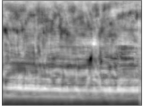
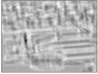
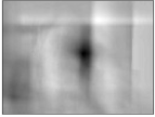
ZNCC(1 tpl)

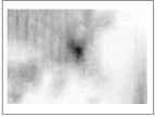
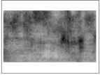
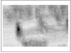
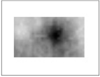
BBS(1 tpl)

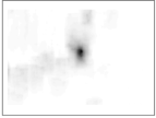
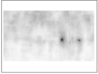
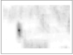
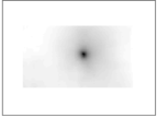
DDIS(1 tpl)

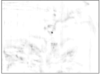
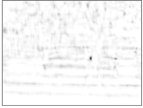
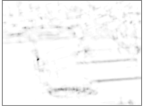
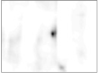
DIM (1 template)

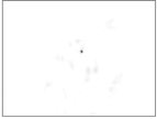
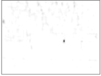
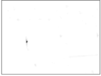
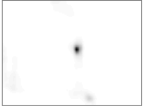
DIM(1 tpl)

Figure 1: Example results for different algorithms when applied to the task of finding corresponding locations in 105 pairs of colour video frames. Images in the first row show the target templates (outlined in yellow) in the initial frame of the video. Images in the second row show the location of the target identified by the DIM algorithm (outlined in cyan) and the location of the target defined by the ground-truth data (outlined in yellow) in a later frame of the same video. The third to seventh rows show the similarity of the target template to the second image as determined by (from row 3 to 7): ZNCC, BBS, DDIS, DIM with no additional templates, and DIM with up to four additional templates chosen by maximum correlation. Darker pixels correspond to stronger similarity. Note, matching was performed using colour templates and colour images, but for clarity the images are shown in grayscale in rows 1 and 2.

Results for typical example image pairs are shown in fig. 1. The images on the top row are the first images in each of four image pairs. The yellow box superimposed on each image shows the target image patch. The second row shows the second image in each pair. Two boxes are superimposed on these second images. The yellow box shows the location corresponding to the target defined by the ground-truth data. The cyan box shows the location of the target predicted by the DIM algorithm. The remaining rows show the similarity between the template and the second image calculated by several different methods. The strongest measures of similarity are represented by the darkest pixels. The similarity array calculated by ZNCC (fig. 1 third row) is dense. The similarity arrays produced by BBS (fig. 1 fourth row), DDIS (fig. 1 fifth row), and DIM (fig. 1 sixth and seventh rows), become increasingly sparse, and hence, the peaks become increasingly well-localised and easily distinguishable from non-matching locations.

Two results are shown for the DIM algorithm. The first result (fig. 1 sixth row) shows the similarity of the target template to the second image when only the target template was used by DIM. The second result for the DIM algorithm (fig. 1 seventh row) shows the similarity calculated when up to four additional templates, the same size as the bounding-box defining the target, were also extracted from the first image and used as templates for non-target locations by DIM. These additional templates were extracted from around locations where the correlation between the target template and the image was strongest, excluding locations where the additional templates would overlap with each other or with the bounding-box defining the target. The exact number of additional templates varied between different image pairs, and in some cases over the 105 image pairs, there were zero additional templates due to the target bounding-box being large compared to the size of the image. For the particular examples shown in fig. 1 all results were produced using four additional templates, except that for the right-most image where two additional templates were used. As can be seen by comparing the sixth and seventh rows of fig. 1, including additional, non-target, templates tends to increase the sparsity of the similarity array produced by DIM for the target template. This increased sparsity results from the increased competition when there are more templates (see sect. 3.2).

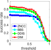
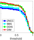
Figure 2: The performance of different algorithms when applied to the task of finding corresponding locations in 105 pairs of colour video frames. Each curve shows the fraction of targets for which the overlap between the ground-truth and predicted bounding-boxes exceeded the threshold indicated on the x-axis. (a) Results when using the target location predicted by the maximum similarity. (b) Results when using the maximum overlap predicted by the seven highest similarity values. The results for DIM are produced using up to four additional templates chosen by maximum correlation.

The results across all 105 image pairs are summarised in fig. 2(a). This graph shows the proportion of image pairs for which the overlap between the ground-truth and the predicted bounding-box (the IoU) exceeded a threshold for a range of different threshold values. It can be seen that the success rate of DIM exceeds that of the other methods at all thresholds. Following the methods used in Dekel et al., (2015), the overall accuracy of each method was summarised using the area under the success curve (AUC). These quantitative results are shown in footnote h, and compared to the published results for several additional algorithms that have been evaluated on the same dataset.

Dekel et al., (2015) also assessed the accuracy of BBS by taking the largest overlap across the seven locations with the highest similarity values. The same analysis was done here by finding the seven largest peaks in the similarity array for the target template, ignoring values that were not local maxima. These results are presented in fig. 2(b). It can be seen that DIM produces similar results to DDIS, but significantly better performance than both ZNCC and BBS over a wide range of threshold values.

Algorithm	AUC
Baseline
SSD	0.43 (Dekel et al.,, 2015)
NCC	0.47 (Dekel et al.,, 2015)
SAD	0.49 (Dekel et al.,, 2015)
ZNCC	0.54
State-of-the-art
BBS (Dekel et al.,, 2015; Oron et al.,, 2018)	0.55 (Dekel et al.,, 2015)
CNN (2ch-deep) (Zagoruyko and Komodakis,, 2015, 2017)	0.59 (Kim et al.,, 2017)
CoTM (Kat et al.,, 2018)	0.62∗ (Kat et al.,, 2018)
CNN (SADCFE) (Kim et al.,, 2017)	0.63 (Kim et al.,, 2017)
CNN (2ch-2stream) (Zagoruyko and Komodakis,, 2015, 2017)	0.63 (Kim et al.,, 2017)
DDIS (Talmi et al.,, 2017)	0.64 (Kat et al.,, 2018)
Proposed
DIM (1 template)	0.58
DIM (1 to 4 templates)	0.69

Table 1: Quantitative comparison of results for different algorithms when applied to the task of finding corresponding locations in 105 pairs of colour video frames. Results are given in terms of the area under the success curve (AUC). ^∗We failed to reproduce the result for CoTM given in (Kat et al.,, 2018): using the code released by the authors to perform the matching, together with our code to run the benchmark, produced an AUC of 0.54. Using the same code for running the benchmark and the code supplied by the original authors it was possible to reproduce the published results for both BBS and DDIS.

From footnote h it can be seen that the performance of DIM is strongly effected by the inclusion of additional templates extracted from other parts of the first image. This is to be expected, as the proposed method performs explaining away, and the accuracy of this inference process will increase when additional templates compete with the target template such that regions of the image that should have low similarity with the target template are explained-away by the additional templates. Without any additional templates the performance of DIM is more similar to ZNCC, this is also to be expected as both methods are comparing the relative intensity values in the template and each patch of image.

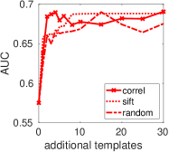
Figure 3: The effect of the maximum number of additional templates, and their selection method, on the performance of the proposed method, DIM, when applied to finding corresponding locations in 105 pairs of colour video frames. Results are shown when the additional templates were selected from (a) the first image in each pair, and (b) an unrelated image.

A number of different methods of choosing the additional, non-target, templates used by DIM were investigated. fig. 3 shows the AUC obtained for different maximum numbers of additional templates, when these templates were selected from locations where the correlation between the target template and the image was strongest, from locations selected by the SIFT interest point detector, and locations chosen at random. In each case, additional templates were chosen such that they did not overlap with each other or with the bounding-box defining the target so as to ensure a diversity of additional templates. The exact number of additional templates varied between different image pairs, depending on how many non-overlapping regions, equal in size to the target template, could fit within the first image in each pair. It can be seen that the performance of DIM increased as the number of non-target templates increased, and that for a large number of additional templates the AUC plateaued between 0.66 and 0.69 regardless of how the additional templates were selected. Furthermore, for all three methods of selecting additional templates the performance of DIM exceeded that of the current state-of-the-art method, DDIS, when two or more additional templates were used. It can also be observed from fig. 3 that the initial increase in performance with the number of additional templates was faster when the non-target templates were chosen by maximum correlation. In other words, the best performance was achieved with fewer additional templates if those additional templates were chosen so that they were the regions of the first image that were most similar to, and hence most easily mistaken for, the target region.

One concern is that the benefits of performing explaining away will disappear when the target appears in a completely different context. In other words, if the background of the first image is different from that for the second image, then additional, non-target, templates extracted from the first image will be ineffective at competing with the target template when they are matched to the second image. To explore this issue, the experiment described in the preceding paragraph was repeated, but the additional templates were taken from an unrelated image (the first “Leuven” image from the Oxford VGG Affine Covariant Features Dataset (Mikolajczyk and Schmid,, 2005; Mikolajczyk et al.,, 2005), see sect. 4.2). The results of this experiment are shown in fig. 3. As expected, there was a deterioration in performance. However, as long as sufficient ($\geq 20$) additional templates were used then the performance of DIM (an AUC of $\geq 64$) was still as good as, or better than, all other methods that have been applied to this benchmark (see footnote h).

4.2 Correspondence using the Oxford VGG Affine Covariant Features Dataset

This section describes an experiment similar to that in sect. 4.1, but using the images from the Oxford VGG Affine Covariant Features Benchmark (Mikolajczyk and Schmid,, 2005; Mikolajczyk et al.,, 2005). This dataset has been widely used to test the ability of interest point detectors to locate corresponding points in two images. The dataset consists of eight image sequences (seven colour and one grayscale). Each sequence consists of six images of the same scene. These images differ in viewpoint (resulting in changes in perspective, orientation, and scale), illumination/exposure, blur/de-focus and JPEG compression. The ground-truth correspondences are defined in terms of homographies (plane projective transformations) which relate any location in the first image of each sequence to its corresponding location in the remaining five images in the same sequence. In this experiment, templates were extracted from the first image in each sequence and the best matching locations were found in each of the remaining five images in the same sequence.

Images were scaled to half their original size to reduce the time taken to perform this experiment. From the first image in each sequence templates were extracted (as described in sect. 3.1). These templates were extracted from around keypoints identified using the Harris corner detector. A keypoint detector was used to identify suitable locations for matching in order to exclude locations that no algorithm could be expected to match such as regions of uniform colour and luminance. The results were not dependent on the particular keypoint detector used. From the first image in each sequence 25 keypoints were chosen after excluding those for which: 1) the bounding box defining the extent of the template was not entirely within the image; 2) the bounding box around the corresponding location in the query image was not entirely within the image; 3) the Manhattan distance between the keypoints was less than 24 pixels, or less than the the size of the bounding box defining the extent of the template (which ever distance was smaller). These criteria for rejecting keypoints ensured that the templates did not fall off the edge of either image in each pair (criteria 1 and 2), and increased the diversity of image features that were being matched (criteria 3).

For the DIM algorithm, no additional templates were used as the 25 templates extracted from the first image competed with each other, and hence, for each template the remaining 24 templates effectively acted as additional templates representing non-target image features.

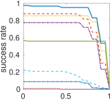
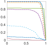
ZNCC

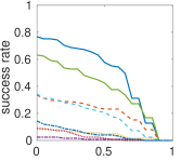
BBS

DDIS

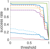
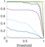
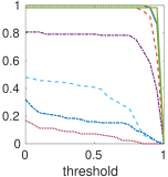
DIM

Figure 4: The performance of different algorithms when applied to the task of finding corresponding locations across image sequences from the Oxford VGG affine covariant features dataset (at half size with 25 templates per image pair). Each curve shows the fraction of targets for which the overlap between the ground-truth and predicted bounding-boxes exceeded the threshold indicated on the x-axis. Results for different image sequences are shown using different line styles, as indicated in the key. Each row shows results for a different algorithm (from top to bottom): ZNCC, BBS, DDIS, and DIM. Each column shows results for a different template size (from left to right): 17-by-17, 33-by-33, and 49-by-49 pixels.

The success curves produced by each algorithm for each sequence are shown in fig. 4, for three different sizes of templates. For all four methods the results generally improved as the template size increased. Differences in appearance between images in the Bikes and Trees sequences are primarily due to changes in image blur. It can be seen from fig. 4 that all four algorithms produced some of their strongest performances when matching locations on these images. The exception was BBS which produced poor performance on the Trees sequence when the template size was small. This is likely to be due to metric used by BBS being insufficiently discriminatory to distinguish distinct locations in the leaves of the trees. Images in the Leuven sequence vary primarily in terms of illumination and exposure. ZNCC and DIM accurately matched points across these images. In contrast, DDIS and BBS showed very little tolerance to illumination changes. Differences in appearance between images in the Wall and Graffiti sequences are primarily due to changes in viewpoint. On the Wall sequence, ZNCC and DIM produced good performance, while DDIS and BBS produced poor performance. In contrast, on the Graffiti sequence DDIS produced the best performance of the four methods. These differences are likely due to the Graffiti sequence having more distinctive image regions, while the Wall images contain many similar looking locations as it is a brick texture. Images in the UBC sequence differ in their JPEG quality. It can be seen from fig. 4 that all four algorithms produced some of their strongest performances when matching locations on these images, except ZNCC and BBS for the small template sizes where the performance was mediocre. Differences in appearance between images in the Bark and Boat sequences are primarily caused by changes in scale and in-plane rotation. Both these sequences were among the most challenging for all four methods. However, the performance for both DDIS and BBS improved as the template size increased.

Algorithm		AUC
patch size (pixels):		17-by-17	33-by-33	49-by-49
ZNCC		0.4996	0.5937	0.6314
BBS (Dekel et al.,, 2015; Oron et al.,, 2018)		0.1782	0.3834	0.4747
DDIS (Talmi et al.,, 2017)		0.3952	0.4905	0.5334
DIM (25 templates)		0.5591	0.6308	0.6569

Table 2: Quantitative comparison of results for different algorithms applied to the task of finding corresponding locations across images in the Oxford VGG affine covariant features dataset (at half size). Results are given in terms of the area under the success curve (AUC) for all 1000 template-image comparisons across all eight sequences in the dataset (25 templates per image pair).

The overall accuracy of each method was summarised using the area under the success curve (AUC) for all 1000 template matches performed (25 templates matched to 5 images in each of 8 sequences). As the same number of template matches were performed for each sequence, this is equivalent to the AUC for the average of the individual success curves for the eight sequences shown in fig. 4. These quantitative results are shown in tab. 2. It can be seen that the proposed method, DIM, significantly out-performs the other methods on this task. Surprisingly, both BBS and DDIS are less accurate than the baseline method, ZNCC.

4.3 Template Matching using the Oxford VGG Affine Covariant Features Dataset

In the preceding two sections template matching algorithms have been evaluated using correspondence tasks. In such tasks it is assumed that the target always appears in the query image. However, in many real-world applications such an assumption is not appropriate, as it is not known if the searched-for image feature appears in the query image. In such applications it is, therefore, not appropriate to select the single location with the highest similarity to the template as the matching location. Instead, it is necessary to apply a threshold to the similarity values to distinguish locations where the template matches the image from those where it does not. To avoid counting multiple matches within a small neighbourhood, it is also typically the case that the similarity must be a local maxima as well as exceeding the global threshold.

To evaluate the ability of the proposed method to perform template matching under these conditions an experiment was performed using the colour images (i.e., excluding the Boat sequence) from the Oxford VGG Affine Covariant Features Benchmark (Mikolajczyk and Schmid,, 2005; Mikolajczyk et al.,, 2005). Only the colour images were used as in this experiment templates extracted from one sequence were matched to images from the other sequences: it was therefore necessary to have all templates and query images either in colour or grayscale. Images were scaled to one-half their original size to reduce the time taken to perform this experiment. From the first image in each sequence 10 templates were extracted from around keypoints identified using the Harris corner detector and using the same criteria as described in sect. 4.2. A total of 70 templates were thus defined (10 for each of the 7 colour sequences). All these 70 templates were matched to each of the 5 query images in each sequence (i.e., to 35 colour images): a total of 2450 template-image comparisons in all.

For every location in the similarity array that was both a local maxima and exceeded a global threshold a bounding box, the same size as the template, was defined in the query image. These locations found by the template matching method were compared to the true location that matched that template in the query image: if the template came from the first image in the same sequence, the comparison was with a bounding box (the same size as the template) defined around the transformed location of the keypoint from around which the template had been extracted; if the template came from a different sequence then there was no matching bounding box in the query image. If the two bounding boxes (one predicted by template matching and one from the ground truth data), had an overlap (IoU) of at least 0.5 this was counted as a true-positive. A ground-truth bounding box not predicted by the template matching process was counted as a false-negative, while matches found by the template matching algorithm that did not correspond to the ground-truth bounding box (or multiple matches to the same ground-truth) were counted as false-positives.

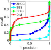
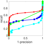
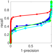
Figure 5: The performance of different algorithms when applied to performing template matching in colour images from the Oxford VGG affine covariant features dataset (at half size). Each curve shows the trade-off between precision and recall for different thresholds applied to the similarity values. A match was considered correct if the bounding box overlap between the predicted location and the true location was at least 0.5. Results are shown for three different sizes of template (a) 17-by-17 pixels, (b) 33-by-33 pixels, and (c) 49-by-49 pixels.

The total number of true-positives ($TP$), false-positives ($FP$), and false-negatives ($FN$) were found for all 70 templates when matched to all 35 query images. These values were then used to calculate recall ($\frac{TP}{TP+FN}$) and precision ($\frac{TP}{TP+FP}$). By varying the global threshold used to define a match, precision-recall curves were plotted to show how detection accuracy varied with threshold. fig. 5 shows the precision-recall curves for each method for three different sizes of templates. The performance of each algorithm was summarised by calculating the f-score ($=2\frac{recall.precision}{recall+precision}=\frac{2TP}{2TP+FP+FN}$) at the threshold that gave the highest value. The f-score measures the best trade-off between precision and recall. The f-scores for each algorithm are shown in tab. 3.

Algorithm		f-score
patch size (pixels):		17-by-17	33-by-33	49-by-49
ZNCC		0.2842	0.5508	0.5493
BBS (Dekel et al.,, 2015; Oron et al.,, 2018)		0.0822	0.3704	0.4579
DDIS (Talmi et al.,, 2017)		0.5198	0.5355	0.4959
DIM (70 templates)		0.6542	0.7230	0.7513

Table 3: Quantitative comparison of results for different algorithms applied to the task of template matching in colour images from the Oxford VGG affine covariant features dataset (at half size). Results are given in terms of the highest f-score for all 2450 template-image comparisons across the seven colour sequences in the dataset (70 templates per image).

From both fig. 5 and tab. 3 it can be seen that the proposed algorithm, DIM, had the best performance. The performance of BBS improved as the template size increased, but at all sizes the performance was well below that of the baseline method, ZNCC. This suggests that the similarity values calculated by BBS vary widely in magnitude such that true and false matches can not be reliably distinguished. The performance of DDIS was similar for all template sizes, but was only superior to that of ZNCC at the smallest size.

4.4 Parameter Sensitivity

The proposed method employs a number of parameters:

• the number of additional templates used;

• the size of the image patches;

• the standard deviation, $\sigma$, of the Gaussian mask used to pre-process the images;

• the value of $\epsilon_{1}$ in equation eq. 3;

• the value of $\epsilon_{2}$ in equation eq. 2;

• The scale factor, $\lambda$, used to determine the size of the elliptical region used to sum neighbouring similarity values;

• the number of iterations performed by the DIM algorithm.

The preceding experiments have already explored the influence of some of these parameters, specifically, the effects of varying the number of additional templates is shown in fig. 3, and the experiments in sect. 4.2 and 4.3 have examined the effects of varying the size of the image patch. Additional experiments were carried out to measure the sensitivity of the proposed algorithm to the other parameters. These experiments applied the algorithm to finding corresponding locations across 105 pairs of colour video frames from the BBS dataset (as in sect. 4.1). In each experiment one parameter was altered at a time while all other parameters were kept fixed at their default values. The results are shown in tab. 4.

It can be seen that the value of $\sigma$ used to pre-process the images could be increased or decreased by a factor of two, and the algorithm still produced performance on this task that exceeded the previous state-of-the-art. However, increasing or decreasing this parameter further had a detrimental effect on performance. This is not surprising as when $\sigma$ is too large or too small $\bar{I}$ becomes a poor estimate of the local image intensity: in the limit $\bar{I}$ becomes equal to the average intensity of the whole image (when $\sigma$ is very large), or $\bar{I}=I$ (when $\sigma$ is very small). In the latter case the input to the template matching method becomes an image where all pixels have a value of zero.

The algorithm was tolerant to large changes in $\epsilon_{1}$, and $\epsilon_{2}$. However, when $\epsilon_{2}$ was increased by a factor of 10 from its default value performance deteriorated. This is becomes this large value of $\epsilon_{2}$ is significant compared to the values of $\mathbf{R}$ (and $\mathbf{X}$), and this causes the DIM algorithm to fail to accurately reconstruct its input, and hence, has non-negligible effects on the steady-state values of $\mathbf{R}$, $\mathbf{E}$ and $\mathbf{Y}$.

Using a very small value of $\lambda$ (which is equivalent to skipping the post-processing stage described in sect. 3.3) resulted in a AUC of 0.687. As shown in tab. 4 larger values of $\lambda$ were beneficial, but if $\lambda$ became too large performance deteriorated. This is because when the summation region is large, small similarity values scattered across a large region of the image can be summed-up to produce what appears to be a strong match from multiple, unrelated, weak matches with the template.

At the end of the first iteration of the DIM algorithm the similarity values are given by: $\mathbf{Y}_{j}=\frac{\epsilon_{1}}{\epsilon_{2}}\odot\sum_{i=1}^{k}\left(\mathbf{w}_{ji}\star\mathbf{X}_{i}\right)$, i.e., the cross-correlation between the templates and the pre-processed image. Hence, unsurprisingly, when only one iteration was performed, performance was very poor and similar to simple correlation-based methods like NCC (compare tab. 4 row “iterations” and column “$\div 10$” with footnote h row “NCC”). Two iterations was also insufficient for the DIM algorithm to find an accurate and sparse representation of the image. However, with between 5 and 50 iterations the proposed method produced accurate results that were consistently equal to or better than those of the previous state-of-the-art. Performance deteriorated when a very large number of iterations was performed. However, this can be offset by increasing the value of $\lambda$. For example, using 100 iterations and $\lambda=0.075$ produced an AUC of 0.666. This can be explained by the similarity values becoming sparser as the number of iterations increases, allowing a larger summation region to be used without such a risk of integrating across unrelated similarity values.

Parameter	Standard	AUC when value changed by:
	Value	$\div 10$	$\div 5$	$\div 2$	$\times 2$	$\times 5$	$\times 10$
$\sigma$ (see sect. 3.1)	0.5min(w,h)	0.536	0.597	0.681	0.674	0.609	0.554
$\epsilon_{1}$ (see eq. 3)	$\frac{\epsilon_{2}}{max\left(\sum_{j}v_{ji}\right)}$	0.688	0.688	0.690	0.690	0.689	0.688
$\epsilon_{2}$ (see eq. 2)	0.01	0.690	0.690	0.690	0.686	0.691	0.624
$\lambda$ (see sect. 3.3)	0.025	0.695	0.695	0.695	0.682	0.682	0.636
iterations (see sect. 3.2)	10	0.451	0.593	0.687	0.668	0.644	0.632

Table 4: Evaluation of the sensitivity of the proposed algorithm to its parameter values. Note, w and h stand for the width and height of the template. Performance was evaluated using the AUC produced for the task of finding corresponding locations in 105 pairs of colour video frames from the BBS dataset (i.e., using the same procedure as used to generate the result shown in footnote h). Using the standard parameter values the AUC is equal to 0.690.

4.5 Computational Complexity

The focus of this work was to develop a more accurate method of template matching. Computational complexity was therefore not of prime concern. However, for completeness, this section provides a comparison of the computational complexity of DIM.

To calculate the cross-correlation or convolution of a $M$-by$N$ pixel image with a $m$-by-$n$ pixel template, requires $mn$ multiplications at each image pixel, so the approximate computational complexity is $O(MNmn)$. In the DIM algorithm, to avoid edge effects, the image is padded by $2m$ in width and $2n$ in height. In this case, the computational complexity of 2D cross-correlation is $O((M+2m)(N+2n)mn)$.

In the DIM algorithm, 2D convolution is applied to calculate the values of $\mathbf{R}$ for each channel (see eq. 1) and 2D cross-correlation is used to calculate the values of $\mathbf{Y}$ for each template (see eq. 3). Both these updates are performed at each of $i$ iterations. So if there are $c$ channels and $t$ templates, then the complexity is approximately $O(2(M+2m)(N+2n)mncti)$. Added to this is the time taken to compute the element-wise division (see eq. 2) and multiplication (see eq. 3) operations at each iteration, which has a complexity of $O(MN(c+t)i)$. However, this is negligible compared to the time taken to perform the cross-correlations and convolutions.

It is well-known that 2D convolution and 2D cross-correlation can be performed in Fourier space with complexity $O(MNlog(MN))$, assuming $m\leq M$ and $n\leq N$. This method is therefore faster when $mn$ is larger than $log((M+2m)(N+2n))$. Using the Fourier method of calculating the cross-correlations and convolutions, the complexity of DIM would be approximately $O(2(M+2m)(N+2n)log(MN)cti)$. Cross-correlation and convolution are inherently parallel processes as each output value is independent of the other output values. Hence, with appropriate multi-core hardware the computational complexity of 2D cross-correlation and 2D convolution becomes $O(mn)$. With such parallel computation, the computational complexity of DIM would be approximately $O(2mni)$, as the value of $\mathbf{R}$ across all channels and the values of $\mathbf{Y}$ for all templates could also be calculated in parallel.

This compares to the complexity of ZNCC which is $O(MNmnct)$ (or $O(mn)$ on parallel hardware); BBS which is $O(MNm^{2}n^{2}ct)$ (Oron et al.,, 2018); and DDIS which is $O(9mnlog(mn)t+MNmnt+MNt(c+log(mn)))$ (Talmi et al.,, 2017). To compare the real-world performance, execution times for each algorithm were recorded on a computer with Intel Core i7-7700K CPU running at 4.20GHz. This machine ran Ubuntu GNU/Linux 16.04 and MATLAB R2017a. All code was written in MATLAB. For DDIS faster, compiled, code is available to reduce execution times on machines running Microsoft Windows. The code for DIM was not compiled for a fair comparison. The total time taken to perform the experiment described in sect. 4.1 (i.e., to perform template matching across 105 colour image pairs), the time taken to perform the experiment described in sect. 4.2 with 17-by-17 pixel templates (i.e., to match 25 templates across 40 image pairs), and the time taken to perform the experiment described in sect. 4.3 with 17-by-17 pixel templates (i.e., to match 70 templates to 35 images) are shown in tab. 5. While DIM is not as fast as the simple, baseline, method it is the fastest of the other methods while also being the most accurate. It also has the potential to be much faster if implemented on appropriate parallel hardware.

Algorithm	Execution Time (s)
ZNCC	15 (0.14)	33 (0.03)	59 (0.02)
BBS (Dekel et al.,, 2015; Oron et al.,, 2018)	2193 (20.89)	724 (0.72)	1512 (0.62)
DDIS (Talmi et al.,, 2017)	4802 (45.73)	17391 (17.39)	40102 (16.37)
DIM	938 (8.93)	209 (0.21)	1366 (0.56)

Table 5: Comparison of the execution times of different algorithms. The first column of times show the total time taken when the algorithms where applied to the task of finding corresponding locations in 105 pairs of colour video frames (i.e., to obtain the results shown in fig. 2). The second column of times are for the task of finding 25 corresponding points in each pair of images from the Oxford VGG affine covariant features dataset, at one-half size, using 17-by-17 pixel templates (i.e., to obtain the results shown in the first column of fig. 4). The third column of times are for the algorithms when applied to the task of matching 70 17-by-17 pixel templates to 35 colour images from the Oxford VGG affine covariant features dataset, at half size (i.e., to obtain the results shown in fig. 5a). The values in brackets are the average times taken to compare one template with one image in each task.

5 Conclusions

This article has evaluated a method of performing template matching that is shown to be both accurate and tolerant to differences in appearance due to viewpoint, variations in background, non-rigid deformations, illumination, blur/de-focus and JPEG compression. This advantageous behaviour is achieved by causing the templates to compete to match the image, using the existing DIM algorithm (Spratling et al.,, 2009; Spratling,, 2017). Specifically, the competition is implemented as a form of probabilistic inference known as explaining away (Kersten et al.,, 2004; Lochmann and Deneve,, 2011; Spratling,, 2012; Spratling et al.,, 2009) which causes each image element to only provide support for the template that is the most likely match. Explaining away produces a sparse array of similarity values in which the peaks are easily identified, and in which similarity values that are reduced in magnitude by differences in appearance are still distinct from those similarity values at non-matching locations. Using a variety of tasks, the proposed method was shown to out-perform traditional template matching, and recent state-of-the-art methods (Talmi et al.,, 2017; Dekel et al.,, 2015; Oron et al.,, 2018; Kat et al.,, 2018; Kim et al.,, 2017; Zagoruyko and Komodakis,, 2015, 2017).

Specifically, the proposed method was compared to the BBS algorithm (Dekel et al.,, 2015; Oron et al.,, 2018), and several other recent methods (Zagoruyko and Komodakis,, 2015, 2017; Kat et al.,, 2018; Kim et al.,, 2017; Talmi et al.,, 2017), using the same dataset and experimental procedures defined by the authors of the BBS algorithm. This task required target objects from one frame of a colour video to be located in a subsequent frame. Changes in the appearance of the target were due to variations in camera viewpoint or the pose of the target, partial occlusions, non-rigid deformations, and changes in the surrounding context, background, and illumination. On this dataset the proposed algorithm produced significantly more accurate results than the BBS algorithm, and more recent algorithms that have been applied to the same dataset (Zagoruyko and Komodakis,, 2015, 2017; Kat et al.,, 2018; Kim et al.,, 2017; Talmi et al.,, 2017). Furthermore, using the Oxford VGG Affine Covariant Features Dataset (Mikolajczyk and Schmid,, 2005; Mikolajczyk et al.,, 2005) it was shown that these findings generalise to other tasks and other images. In this second set of images, changes in the appearance of the target were due to variations in camera viewpoint, illumination/exposure, blur/de-focus, and JPEG compression. The proposed method considerably outperformed some recently proposed state-of-the-art methods (Dekel et al.,, 2015; Oron et al.,, 2018; Talmi et al.,, 2017) on these additional experiments.

The present results demonstrate that the proposed method is tolerant to a range of factors that cause differences between the template and the target as it appears in the query image. However, it is only weakly tolerant to changes in appearance caused by viewpoint (i.e., changes in perspective, orientation, and scale). The tolerance of DIM to viewpoint changes could, potentially, be improved using a number of techniques.

Firstly, by using additional templates representing transformed versions of the searched-for image patch. For example, to recognise a patch of image at a range of orientations it would be possible to include additional templates showing that patch at different orientations. The final similarity measure at each image location would then be determined by finding the maximum of the similarity values calculated for each individual template representing transformed versions of the same template at that location. Additional, unreported, experiments have shown that this method works well. However, to deal with an unknown transformation between the template and the query image it is necessary to use a large number of affine transformed templates showing many possible combinations of changes in scale, rotation and shear, and hence, this method is computationally expensive and not very practical.

Secondly, it would be possible to split templates into multiple sub-templates. The sub-templates could be matched to the image, using DIM, and each one could vote for the location of the target. By allowing some tolerance in the range of sub-template locations that vote for the same target location, this method could provide additional tolerance to changes in appearance, particularly changes caused by image shear and changes in perspective. Essentially, this method would perform template matching using an algorithm analogous to the implicit shape model (ISM; Leibe et al.,, 2008), which employs the generalised Hough transform (Ballard,, 1981; Duda and Hart,, 1972). Both the sub-template matching and the votong processes could be implemented using the DIM algorithm (Spratling,, 2017; Spratling, 2016a, ).

Thirdly, it would be possible to apply the method to a different feature-space, one in which the features were tolerant to changes in appearance. It has been shown that for other methods significant improvement in performance can be achieved by applying the method to a feature-space defined by the output of certain layers in a CNN (Kim et al.,, 2017; Kat et al.,, 2018; Talmi et al.,, 2017). For example, Kim et al., (2017) showed that applying NCC to features extracted by a CNN, in comparison to using NCC to compare colour intensity values, produced an increase of 0.15 in the AUC for the experiment described in sect. 4.1. An obvious direction for future work on the proposed algorithm is to apply it to a similar feature-space extracted by a deep neural network.

In terms of practical applications, the proposed method has already been applied, as part of a hierarchical DIM network, to object localisation and recognition (Spratling,, 2017) and to the low-level task of edge-detection (Spratling,, 2013; Wang and Spratling,, 2016). Future work might also usefully explore applications of the proposed method to stereo correspondence, 3D reconstruction, and tracking. To facilitate such future work all the code used to produce the results reported in this article has been made freely available.

References

- Achler, (2014) Achler, T. (2014). Symbolic neural networks for cognitive capacities. Biologically Inspired Cognitive Architectures, 9:71–81.
- Ballard, (1981) Ballard, D. H. (1981). Generalizing the Hough transform to detect arbitrary shapes. Pattern Recognition, 13(2):111–22.
- (3) Balntas, V., Johns, E., Tang, L., and Mikolajczyk, K. (2017a). Pn-net: conjoined triple deep network for learning local image descriptors. arXiv:1601.05030.
- (4) Balntas, V., Lenc, K., Vedaldi, A., and Mikolajczyk, K. (2017b). HPatches: A benchmark and evaluation of handcrafted and learned local descriptors. In Proceedings of the IEEE Computer Society Conference on Computer Vision and Pattern Recognition.
- Balntas et al., (2016) Balntas, V., Riba, E., Ponsa, D., and Mikolajczyk, K. (2016). Learning local feature descriptors with triplets and shallow convolutional neural networks. In Proceedings of the British Machine Vision Conference.
- Balntas et al., (2018) Balntas, V., Tang, L., and Mikolajczyk, K. (2018). Binary online learned descriptors. IEEE Transactions on Pattern Analysis and Machine Intelligence, 40(3).
- Barnea and Silverman, (1972) Barnea, D. I. and Silverman, H. F. (1972). A class of algorithms for fast digital image registration. IEEE Transactions on Computers, C-21(2):179–86.
- Bay et al., (2006) Bay, H., Tuytelaars, T., and Gool, L. V. (2006). SURF: Speeded up robust features. In Proceedings of the European Conference on Computer Vision.
- Beyeler et al., (2019) Beyeler, M., Rounds, E. L., Carlson, K. D., Dutt, N., and Krichmar, J. L. (2019). Neural correlates of sparse coding and dimensionality reduction. PLOS Computational Biology, 15(6):1–33.
- Brown et al., (2011) Brown, M., Hua, G., and Winder, S. (2011). Discriminative learning of local image descriptors. IEEE Transactions on Pattern Analysis and Machine Intelligence, 33(1):43–57.
- Brown and Lowe, (2007) Brown, M. and Lowe, D. G. (2007). Automatic panoramic image stitching using invariant features. International Journal of Computer Vision, 74(1):59–73.
- Brown et al., (2003) Brown, M. Z., Burschka, D., and Hager, G. D. (2003). Advances in computational stereo. IEEE Transactions on Pattern Analysis and Machine Intelligence, 25(8):993–1008.
- Calonder et al., (2010) Calonder, M., Lepetit, V., Strecha, C., and Fua, P. (2010). BRIEF: Binary robust independent elementary features. In Proceedings of the European Conference on Computer Vision.
- Canny, (1986) Canny, J. F. (1986). A computational approach to edge detection. IEEE Transactions on Pattern Analysis and Machine Intelligence, 8:679–98.
- Comaniciu et al., (2000) Comaniciu, D., Ramesh, V., and Meer, P. (2000). Real-time tracking of non-rigid objects using mean shift. In Proceedings of the IEEE Computer Society Conference on Computer Vision and Pattern Recognition, pages 142–9.
- Csurka et al., (2004) Csurka, G., Dance, C., Fan, L., Willamowski, J., and Bray, C. (2004). Visual categorization with bags of keypoints. In Proceedings of the European Conference on Computer Vision. Workshop on Statistical Learning for Computer Vision.
- Dalal and Triggs, (2005) Dalal, N. and Triggs, B. (2005). Histograms of oriented gradients for human detection. In Proceedings of the IEEE Computer Society Conference on Computer Vision and Pattern Recognition, pages 886–93.
- Dekel et al., (2015) Dekel, T., Oron, S., Rubinstein, M., Avidan, S., and Freeman, W. T. (2015). Best-buddies similarity for robust template matching. In Proceedings of the IEEE Computer Society Conference on Computer Vision and Pattern Recognition, pages 2021–9.
- Dong and Soatto, (2015) Dong, J. and Soatto, S. (2015). Domain-size pooling in local descriptors: DSP-SIFT. In Proceedings of the IEEE Computer Society Conference on Computer Vision and Pattern Recognition.
- Duda and Hart, (1972) Duda, R. O. and Hart, P. E. (1972). Use of the Hough transformation to detect lines and curves in pictures. Communications of the ACM, 15(1):11–5.
- Gall et al., (2011) Gall, J., Yao, A., Razavi, N., Van Gool, L., and Lempitsky, V. (2011). Hough forests for object detection, tracking, and action recognition. IEEE Transactions on Pattern Analysis and Machine Intelligence, 33(11):2188–202.
- Girshick et al., (2016) Girshick, R., Donahue, J., Darrell, T., and Malik, J. (2016). Region-based convolutional networks for accurate object detection and segmentation. IEEE Transactions on Pattern Analysis and Machine Intelligence, 38(1):142–58.
- Goshtasby et al., (1984) Goshtasby, A., Gage, S. H., and Bartholic, J. F. (1984). A two-stage cross correlation approach to template matching. IEEE Transactions on Pattern Analysis and Machine Intelligence, 6(3):374–8.
- Gu et al., (2009) Gu, C., Lim, J. J., Arbelaez, P., and Malik, J. (2009). Recognition using regions. In Proceedings of the IEEE Computer Society Conference on Computer Vision and Pattern Recognition, pages 1030–7.
- Hoyer, (2004) Hoyer, P. O. (2004). Non-negative matrix factorization with sparseness constraints. Journal of Machine Learning Research, 5:1457–69.
- Kat et al., (2018) Kat, R., Jevnisek, R., and Avidan, S. (2018). Matching pixels using co-occurrence statistics. In Proceedings of the IEEE Computer Society Conference on Computer Vision and Pattern Recognition.
- Kersten et al., (2004) Kersten, D., Mamassian, P., and Yuille, A. (2004). Object perception as Bayesian inference. Annual Review of Psychology, 55(1):271–304.
- Khan et al., (2015) Khan, N., McCane, B., and Mills, S. (2015). Better than SIFT? Machine Vision and Applications, 26(6):819–36.
- Kim et al., (2017) Kim, J., Kim, J., Choi, S., Hasan, M. A., and Kim, C. (2017). Robust template matching using scale-adaptive deep convolutional features. In Proceedings of the Asia-Pacific Signal and Information Processing Association Annual Summit and Conference (APSIPA ASC), pages 708–11, Malaysia.
- Korman et al., (2018) Korman, S., Milam, M., and Soatto, S. (2018). OATM: Occlusion aware template matching by consensus set maximization. In Proceedings of the IEEE Computer Society Conference on Computer Vision and Pattern Recognition.
- Korman et al., (2013) Korman, S., Reichman, D., Tsur, G., and Avidan, S. (2013). FAsT-Match: Fast affine template matching. In Proceedings of the IEEE Computer Society Conference on Computer Vision and Pattern Recognition, pages 2331–8.
- Kwang et al., (2016) Kwang, M., Trulls, E., Lepetit, V., and Fua, P. (2016). LIFT: Learned invariant feature transform. In Proceedings of the European Conference on Computer Vision.
- Lampert et al., (2008) Lampert, C., Blaschko, M., and Hofmann, T. (2008). Beyond sliding windows: Object localization by efficient subwindow search. In Proceedings of the IEEE Computer Society Conference on Computer Vision and Pattern Recognition.
- Lee and Seung, (1999) Lee, D. D. and Seung, H. S. (1999). Learning the parts of objects by non-negative matrix factorization. Nature, 401:788–91.
- Lee and Seung, (2001) Lee, D. D. and Seung, H. S. (2001). Algorithms for non-negative matrix factorization. In Leen, T. K., Dietterich, T. G., and Tresp, V., editors, Advances in Neural Information Processing Systems, volume 13, Cambridge, MA. MIT Press.
- Leibe et al., (2008) Leibe, B., Leonardis, A., and Schiele, B. (2008). Robust object detection with interleaved categorization and segmentation. International Journal of Computer Vision, 77(1-3):259–89.
- Lepetit and Fua, (2006) Lepetit, V. and Fua, P. (2006). Keypoint recognition using randomized trees. IEEE Transactions on Pattern Analysis and Machine Intelligence, 28(9):1465–79.
- Lochmann and Deneve, (2011) Lochmann, T. and Deneve, S. (2011). Neural processing as causal inference. Current Opinion in Neurobiology, 21(5):774–81.
- Lowe, (1999) Lowe, D. G. (1999). Object recognition from local scale-invariant features. In Proceedings of the International Conference on Computer Vision, pages 1150–7.
- Lowe, (2004) Lowe, D. G. (2004). Distinctive image features from scale-invariant keypoints. International Journal of Computer Vision, 60(2):91–110.
- Lucas and Kanade, (1981) Lucas, B. and Kanade, T. (1981). An iterative image registration technique with an application to stereo vision. In Proceedings of the International Joint Conference on Artificial Intelligence, pages 674–9.
- Ma et al., (2009) Ma, L., Sun, Y., Feng, N., and Liu, Z. (2009). Image fast template matching algorithm based on projection and sequential similarity detecting. In Fifth International Conference on Intelligent Information Hiding and Multimedia Signal Processing, pages 957–60.
- Mikolajczyk and Schmid, (2005) Mikolajczyk, K. and Schmid, C. (2005). A performance evaluation of local descriptors. IEEE Transactions on Pattern Analysis and Machine Intelligence, 10(27):1615–30.
- Mikolajczyk et al., (2005) Mikolajczyk, K., Tuytelaars, T., Schmid, C., Zisserman, A., Matas, J., Schaffalitzky, F., Kadir, T., and Gool, L. V. (2005). A comparison of affine region detectors. International Journal of Computer Vision, 65(1/2):43–72.
- Mitra et al., (2017) Mitra, R., Zhang, J., Narayan, S., Ahmed, S., Chandran, S., and Jain, A. (2017). Improved descriptors for patch matching and reconstruction. In ICCV Workshop on Compact and Efficient Feature Representation and Learning.
- Morel and Yu, (2009) Morel, J. M. and Yu, G. (2009). ASIFT: a new framework for fully affine invariant image comparison. SIAM Journal on Imaging Sciences, 2(2):438–69.
- Muhammad and Spratling, (2015) Muhammad, W. and Spratling, M. W. (2015). A neural model of binocular saccade planning and vergence control. Adaptive Behavior, 23(5):265–82.
- Mukherjee et al., (2015) Mukherjee, D., Jonathan Wu, Q., and Wang, G. (2015). A comparative experimental study of image feature detectors and descriptors. Machine Vision and Applications, 26(4):443–66.
- Oron et al., (2018) Oron, S., Dekel, T., Xue, T., Freeman, W. T., and Avidan, S. (2018). Best-buddies similarity; robust template matching using mutual nearest neighbors. IEEE Transactions on Pattern Analysis and Machine Intelligence, 40(8):1799–813.
- Özuysal et al., (2010) Özuysal, M., Calonder, M., Lepetit, V., and Fua, P. (2010). Fast keypoint recognition using random ferns. IEEE Transactions on Pattern Analysis and Machine Intelligence, 32(3):448–61.
- Rublee et al., (2011) Rublee, E., Rabaud, V., Konolige, K., and Bradski, G. (2011). ORB: An efficient alternative to SIFT or SURF. In Proceedings of the International Conference on Computer Vision, pages 2564–71.
- Saleiro et al., (2017) Saleiro, M., Terzić, K., Rodrigues, J., and du Buf, J. (2017). BINK: Biological binary keypoint descriptor. Biosystems, 162:147–56.
- Schönberger et al., (2017) Schönberger, J. L., Hardmeier, H., Sattler, T., and Pollefeys, M. (2017). Comparative evaluation of hand-crafted and learned local features. In Proceedings of the IEEE Computer Society Conference on Computer Vision and Pattern Recognition.
- Se et al., (2005) Se, S., Lowe, D. G., and Little, J. J. (2005). Vision-based global localization and mapping for mobile robots. IEEE Transactions on Robotics, 21(3):364–75.
- Simo-Serra et al., (2015) Simo-Serra, E., Trulls, E., Ferraz, L., Kokkinos, I., Fua, P., and Moreno-Noguer, F. (2015). Discriminative learning of deep convolutional feature point descriptors. In Proceedings of the International Conference on Computer Vision.
- Simonyan et al., (2014) Simonyan, K., Vedaldi, A., and Zisserman, A. (2014). Learning local feature descriptors using convex optimisation. IEEE Transactions on Pattern Analysis and Machine Intelligence, 36(8):1573–85.
- Solbakken and Junge, (2011) Solbakken, L. L. and Junge, S. (2011). Online parts-based feature discovery using competitive activation neural networks. In Proceedings of the International Joint Conference on Neural Networks, pages 1466–73.
- Spratling, (2011) Spratling, M. W. (2011). A single functional model accounts for the distinct properties of suppression in cortical area V1. Vision Research, 51(6):563–76.
- Spratling, (2012) Spratling, M. W. (2012). Unsupervised learning of generative and discriminative weights encoding elementary image components in a predictive coding model of cortical function. Neural Computation, 24(1):60–103.
- Spratling, (2013) Spratling, M. W. (2013). Image segmentation using a sparse coding model of cortical area V1. IEEE Transactions on Image Processing, 22(4):1631–43.
- Spratling, (2014) Spratling, M. W. (2014). Classification using sparse representations: a biologically plausible approach. Biological Cybernetics, 108(1):61–73.
- (62) Spratling, M. W. (2016a). A neural implementation of the Hough transform and the advantages of explaining away. Image and Vision Computing, 52:15–24.
- (63) Spratling, M. W. (2016b). Predictive coding as a model of cognition. Cognitive Processing, 17(3):279–305.
- Spratling, (2017) Spratling, M. W. (2017). A hierarchical predictive coding model of object recognition in natural images. Cognitive Computation, 9(2):151–67.
- Spratling et al., (2009) Spratling, M. W., De Meyer, K., and Kompass, R. (2009). Unsupervised learning of overlapping image components using divisive input modulation. Computational Intelligence and Neuroscience, 2009(381457):1–19.
- Szeliski, (2006) Szeliski, R. (2006). Image alignment and stitching: A tutorial. Foundations and Trends in Computer Graphics and Vision, 2(1):1–104.
- Talmi et al., (2017) Talmi, I., Mechrez, R., and Zelnik-Manor, L. (2017). Template matching with deformable diversity similarity. In Proceedings of the IEEE Computer Society Conference on Computer Vision and Pattern Recognition, pages 1311–9.
- Tareen and Saleem, (2018) Tareen, S. A. K. and Saleem, Z. (2018). A comparative analysis of SIFT, SURF, KAZE, AKAZE, ORB, and BRISK. In International Conference on Computing, Mathematics and Engineering Technologies (iCoMET), pages 1–10.
- Tola et al., (2008) Tola, E., Lepetit, V., and Fua, P. (2008). A fast local descriptor for dense matching. In Proceedings of the IEEE Computer Society Conference on Computer Vision and Pattern Recognition, pages 1–8.
- Trzcinski et al., (2012) Trzcinski, T., Christoudias, M., Lepetit, V., and Fua, P. (2012). Learning image descriptors with the boosting-trick. In Advances in Neural Information Processing Systems.
- Uijlings et al., (2013) Uijlings, J. R. R., van de Sande, K. E. A., Gevers, T., and Smeulders, A. W. M. (2013). Selective search for object recognition. International Journal of Computer Vision, 104(2):154–71.
- Wang and Spratling, (2016) Wang, Q. and Spratling, M. (2016). Contour detection in colour images using a neurophysiologically inspired model. Cognitive Computation, 8(6):1027–35.
- Wei and Lai, (2008) Wei, S. D. and Lai, S. H. (2008). Fast template matching based on normalized cross correlation with adaptive multilevel winner update. IEEE Transactions on Image Processing, 17(11):2227–35.
- (74) Wu, J., Cui, Z., Sheng, V. S., Zhao, P., Su, D., and Gong, S. (2013a). A comparative study of SIFT and its variants. Measurement Science Review, 13(3).
- (75) Wu, Y., Lim, J., and Yang, M.-H. (2013b). Online object tracking: A benchmark. In Proceedings of the IEEE Computer Society Conference on Computer Vision and Pattern Recognition, pages 2411–8.
- Zagoruyko and Komodakis, (2015) Zagoruyko, S. and Komodakis, N. (2015). Learning to compare image patches via convolutional neural networks. In Proceedings of the IEEE Computer Society Conference on Computer Vision and Pattern Recognition, pages 4353–61.
- Zagoruyko and Komodakis, (2017) Zagoruyko, S. and Komodakis, N. (2017). Deep compare: A study on using convolutional neural networks to compare image patches. Computer Vision and Image Understanding, 164:38–55. Deep Learning for Computer Vision.
- Zhang and Akashi, (2015) Zhang, C. and Akashi, T. (2015). Fast affine template matching over galois field. In Xie, X., Jones, M. W., and Tam, G. K. L., editors, Proceedings of the British Machine Vision Conference, pages 121.1–121.11. BMVA Press.
- Zitová and Flusser, (2003) Zitová, B. and Flusser, J. (2003). Image registration methods: a survey. Image and Vision Computing, 21(11):977–1000.