Program Synthesis by Type-Guided Abstraction Refinement

Abstract.

We consider the problem of type-directed component based synthesis where, given a set of (typed) components and a query type, the goal is to synthesize a term that inhabits the query. Classical approaches based on proof search in intuitionistic logics do not scale up to the standard libraries of modern languages, which span hundreds or thousands of components. Recent graph reachability based methods proposed for languages like Java do scale, but only apply to monomorphic data and components: polymorphic data and components infinitely explode the size of the graph that must be searched, rendering synthesis intractable. We introduce type-guided abstraction refinement (TYGAR), a new approach for scalable type-directed synthesis over polymorphic datatypes and components. Our key insight is that we can overcome the explosion by building a graph over abstract types which represent a potentially unbounded set of concrete types. We show how to use graph reachability to search for candidate terms over abstract types, and introduce a new algorithm that uses proofs of untypeability of ill-typed candidates to iteratively refine the abstraction until a well-typed result is found. We have implemented TYGAR in H+, a tool that takes as input a set of Haskell libraries and a query type, and returns a Haskell term that uses functions from the provided libraries to implement the query type. We have evaluated H+ on a set of 44 queries using a set of popular Haskell libraries with a total of 291 components. Our results demonstrate that H+ returns an interesting solution within the first five results for 32 out of 44 queries. Moreover, TYGAR allows H+ to rapidly return well-typed terms, with the median time to first solution of just 1.4 seconds.

1. Introduction

Consider the task of implementing a function firstJust def mbs, which extracts the first non-empty value from a list of options mbs, and if none exists, returns a default value def. Rather than writing a recursive function, you suspect you can implement it more concisely and idiomatically using components from a standard library. If you are a Haskell programmer, at this point you will likely fire up Hoogle (Mitchell, 2004), the Haskell’s API search engine, and query it with the intended type of firstJust, i.e. a $\rightarrow$ [Maybe a] $\rightarrow$ a. The search results will be disappointing, however, since no single API function matches this type. In fact, to implement firstJust you need a snippet that composes three library functions from the standard Data.Maybe library, like so: \def mbs $\rightarrow$ fromMaybe def (listToMaybe (catMaybes mbs)). Wouldn’t you like a tool that could automatically synthesize such snippets from type queries?

Scalable Synthesis via Graph Reachability. In general, our problem of type-directed component-based synthesis, reduces to that of finding inhabitants for a given query type (Urzyczyn, 1997). Consequently, one approach is to develop synthesizers based on proof search in intuitionistic logics (Augusstson, 2005). However, search becomes intractable in the presence of libraries with hundreds or thousands of components. Several papers address the issue of scalability by rephrasing the problem as one of reachability in a type transition network (TTN), i.e. a graph that encodes the library of components. Each type is represented as a state, and each component is represented as a directed transition from the component’s input type to its output type. The synthesis problem then reduces to finding a path in the network that begins at the query’s input type and ends at the output type (Mandelin et al., 2005). To model components (functions) that take multiple inputs, we need only generalize the network to a Petri net which has hyper-transitions that link multiple input states with a single output. With this generalization, the synthesis problem can, once again, be solved by finding a path from the query’s input types to the desired output yielding a scalable synthesis method for Java (Feng et al., 2017).

Challenge: Polymorphic Data and Components. Graph-based approaches crucially rely on the assumption that the size of the TTN is finite (and manageable). This assumption breaks down in the presence of polymorphic components that are ubiquitous in libraries for modern functional languages. (a) With polymorphic datatypes the set of types that might appear in a program is unbounded: for example, two type constructors [] and Int give rise to an infinite set of types (Int, [Int], [[Int]], etc). (b) Even if we bound the set of types, polymorphic components lead to a combinatorial explosion in the number of transitions: for example, the pair constructor with the type a $\rightarrow$ b $\rightarrow$ (a,b) creates a transition from every pair of types in the system. In other words, polymorphic data and components explode the size of the graph that must be searched, rendering synthesis intractable.

Type-Guided Abstraction Refinement. In this work we introduce type-guided abstraction refinement (TYGAR), a new approach to scalable type-directed synthesis over polymorphic datatypes and components. A high-level view of TYGAR is depicted in Fig. 1. The algorithm maintains an abstract transition network (ATN) that finitely overapproximates the infinite network comprising all monomorphic instances of the polymorphic data and components. We use existing SMT-based techniques to find a suitable path in the compact ATN, which corresponds to a candidate term. If the term is well-typed, it is returned as the solution. Due to the overapproximation, however, the ATN can contain spurious paths, which correspond to ill-typed terms. In this case, the ATN is refined in order to exclude this spurious path, along with similar ones. We then repeat the search with the refined ATN until a well-typed solution is found. As such, TYGAR extends synthesis using abstraction refinement (SYNGAR) (Wang et al., 2018), from the domain of values to the domain of types. TYGAR’s support for polymorphism also allows us to handle higher-order components, which take functions as input, by representing functions (arrows) as a binary type constructor. Similarly, TYGAR can handle Haskell’s ubiquitous type classes, by following the dictionary-passing translation (Wadler and Blott, 1989), which again, relies crucially on support for parametric polymorphism.

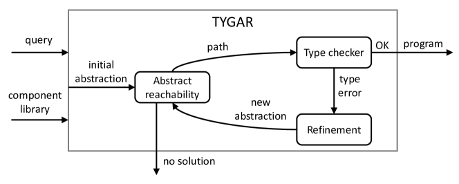
Figure 1. Overview of the TYGAR synthesis algorithm.

Contributions. In summary, this paper makes the following contributions:

1. Abstract Typing. Our first contribution is a novel notion of abstract typing grounded in the framework of abstract interpretation (Cousot and Cousot, 1977). Our abstract domain is parameterized by a finite collection of polymorphic types, each of which abstracts a potentially infinite set of ground instances. Given an abstract domain, we automatically derive an over-approximate type system, which we use to build the ATN. This is inspired by predicate abstraction (Graf and Saidi, 1997), where the abstract domain is parameterized by a set of predicates, and abstract program semantics at different levels of detail can be derived automatically from the domain.

2. Type Refinement. Our second contribution is a new algorithm that, given a spurious program, refines the abstract domain so that the program no longer type-checks abstractly. To this end, the algorithm constructs a compact proof of untypeability of the program: it annotates each subterm with a type that is just precise enough to refute the program.

3. H+. Our third contribution is an implementation of TYGAR in H+, a tool that takes as input a set of Haskell libraries and a type, and returns a ranked list of straight-line programs that have the desired type and can use any function from the provided libraries. To keep in line with Hoogle’s user interaction model familiar to Haskell programmers, H+ does not require any user input beyond the query type; this is in contrast to prior work on component-based synthesis (Feng et al., 2017; Shi et al., 2019), where the programmer provides input-output examples to disambiguate their intent. This setting poses an interesting challenge: given that there might be hundreds of programs of a given type (including nonsensical ones like head []), how do we select just the relevant programs, likely to be useful to the programmer? We propose a novel mechanism for filtering out irrelevant programs using GHC’s demand analysis (Sergey et al., 2017) to eliminate terms where some of the inputs are unused.

We have evaluated H+ on a set of 44 queries collected from different sources (including Hoogle and StackOverflow), using a set of popular Haskell libraries with a total of 291 components. Our evaluation shows that H+ is able to find a well-typed program for 43 out of 44 queries within the timeout of 60 seconds. It finds the first well-typed program within 1.4 seconds on average. In 32 out of 44 queries, the top five results contains a useful solution. Further, our evaluation demonstrates that both abstraction and refinement are important for efficient synthesis. A naive approach that does not use abstraction and instead instantiates all polymorphic datatypes up to even a small depth of 1 yields a massive transition network, and is unable to solve any benchmarks within the timeout. On the other hand, an approach that uses a fixed small ATN but no refinement works well on simple queries, but fails to scale as the solutions get larger. Instead, the best performing search algorithm uses TYGAR to start with a small initial ATN and gradually extend it, up to a given size bound, with instances that are relevant for a given synthesis query.

2. Background and Overview

We start with some examples that illustrate the prior work on component-based synthesis that H+ builds on (Sec. 2.1), the challenges posed by polymorphic components, and our novel techniques for addressing those challenges.

2.1. Synthesis via Type Transition Nets

The starting point of our work is SyPet (Feng et al., 2017), a component-based synthesizer for Java. Let us see how SyPet works by using the example query from the introduction: a $\rightarrow$ [Maybe a] $\rightarrow$ a. For the sake of exposition, we assume that our library only contains three components listed in Fig. 2 (left). Hereafter, we will use Greek letters $\alpha,\beta,\ldots$ to denote existential type variables—i.e. the type variables of components, which have to be instantiated by the synthesizer—as opposed to $a,b,\ldots$ for universal type variables found in the query, which, as far as the synthesizer is concerned, are just nullary type constructors. Since SyPet does not support polymorphic components, let us assume for now that an oracle provided us with a small set of monomorphic types that suffice to answer this query, namely, a, Maybe a, Maybe (Maybe a), [a], and [Maybe a]. For the rest of this section, we abbreviate the names of components and type constructors to their first letter (for example, we will write L (M a) for [Maybe a]) and refer to the query arguments as x1, x2.

⬇

-- | Value stored in the option

-- or default if the option is empty

fromMaybe :: $\alpha$ $\rightarrow$ Maybe $\alpha$ $\rightarrow$ $\alpha$

-- | All values from a list of options

catMaybes :: List (Maybe $\alpha$) $\rightarrow$ List $\alpha$

-- | Head of the list

-- or empty option if the list is empty

listToMaybe :: List $\alpha$ $\rightarrow$ Maybe $\alpha$

Figure 2. (left) A tiny component library. (right) A Type Transition Net for this library and query a $\rightarrow$ List (Maybe a) $\rightarrow$ a. The transitions l<a>, f<a> (resp. l<M a>, f<M a>) correspond to the polymorphic instances of the components listToMaybe, fromMaybe at type a (resp. M a).

Components as Petri Nets. SyPet uses a Petri-net representation of the search space, which we refer to as the type transition net (TTN). The TTN for our running example is shown in Fig. 2 (right). Here places (circles) correspond to types, transitions (rectangles) correspond to components, and edges connect components with their input and output types. Since a component might require multiple inputs of the same type, edges can be annotated with multiplicities (the default multiplicity is 1). A marking of a TTN assigns a non-negative number of tokens to every place. The TTN can step from one marking to the next by firing a transition: if the input places of a transition have sufficiently many tokens, the transition can fire, consuming those input tokens and producing a token in the output place. For example, given the marking in Fig. 2, transition c can fire, consuming the token in L (M a) and producing one in L a; however transition f<a> cannot fire as there is no token in M a.

Synthesis via Petri-Net Reachability. Given a synthesis query $T_{1}\to\ldots\to T_{n}\to T$, we set the initial marking of the TTN to contain one token for each input type $T_{i}$, and the final marking to contain a single token in the type $T$. The synthesis problem then reduces to finding a valid path, i.e. a sequence of fired transitions that gets the net from the initial marking to the final marking. Fig. 2 shows the initial marking for our query, and also indicates the final marking with a double border around the return type a (recall that the final marking of a TTN always contains a single token in a given place). The final marking is reachable via the path ${{{[\mbox{\leavevmode\lstinline{{\lst@@@set@language\lst@@@set@numbers\lst@@@set@frame\lst@@@set@rulecolor\lst@@@set@language\lst@@@set@numbers\lst@@@set@language{\@listingGroup{ltx_lst_identifier}{c}}}}}},\mbox{\leavevmode\lstinline{{\lst@@@set@language\lst@@@set@numbers\lst@@@set@frame\lst@@@set@rulecolor\lst@@@set@language\lst@@@set@numbers\lst@@@set@language{\@listingGroup{ltx_lst_identifier}{l}}}}}},\mbox{\leavevmode\lstinline{{\lst@@@set@language\lst@@@set@numbers\lst@@@set@frame\lst@@@set@rulecolor\lst@@@set@language\lst@@@set@numbers\lst@@@set@language{\@listingGroup{ltx_lst_identifier}{f}}}}}}]$, marked with thick arrows, which corresponds to a well-typed program f x1 (l (c x2)). In general, a path might correspond to multiple programs—if several tokens end up in the same place at any point along the path—of which at least one is guaranteed to be well-typed; the synthesizer can then find the well-typed program using explicit or symbolic enumeration.

2.2. Polymorphic Synthesis via Abstract Type Transition Nets

Libraries for modern languages like Haskell provide highly polymorphic components that can be used at various different instances. For example, our universe contains three type constructors—a, L, and M—which can give rise to infinitely many types, so creating a place for each type is out of question. Even if we limit ourselves to those constructors that are reachable from the query types by following the components, we might still end up with an infinite set of types: for example, following head :: List $\alpha$ $\rightarrow$ $\alpha$ backwards from a yields L a, L (L a), and so on. This poses a challenge for Petri-net based synthesis: which finite set of (monomorphic) instances do we include in the TTN?

On the one hand, we have to be careful not to include too many instances. In the presence of polymorphic components, these instances can explode the number of transitions. Fig. 2 illustrates this for the f and l components, each giving rise to two transitions, by instantiating their type variable $\alpha$ with two different TTN places, a and Maybe a. This proliferation of transitions is especially severe for components with multiple type variables. On the other hand, we have to be careful not to include too few instances. We cannot, for example, just limit ourselves to the monomorphic types that are explicitly present in the query (a and L (M a)), as this will preclude the synthesis of terms that generate intermediate values of some other type, e.g. L a as returned by the component c, thereby preventing the synthesizer from finding solutions.

Abstract Types. To solve this problem, we introduce the notion of an abstract type, which stands for (infinitely) many monomorphic instances. We represent abstract types simply as polymorphic types, i.e. types with free type variables. For example, the abstract type $\tau$ stands for the set of all types, while L $\tau$ stands for the set ${\{\mbox{\leavevmode\lstinline{{\lst@@@set@language\lst@@@set@numbers\lst@@@set@frame\lst@@@set@rulecolor\lst@@@set@language\lst@@@set@numbers\lst@@@set@language{\@listingGroup{ltx_lst_identifier}{L}}}}}}~{}t\mid t\in Type\}$. This representation supports different levels of detail: for example, the type L (M a) can be abstracted into itself, L (M $\tau$), L $\tau$, or $\tau$.

Abstract Transition Nets. A Petri net constructed out of abstract types, which we dub an abstract transition net (ATN), can finitely represent all types in our universe, and hence all possible solutions to the synthesis problem. The ATN construction is grounded in the theory of abstract interpretation and ensures that the net soundly over-approximates the concrete type system, i.e. that every well-typed program corresponds to some valid path through the ATN. Fig. 3 (2) shows the ATN for our running example with places $\tau$, L $\tau$ and a. In this ATN, the rightmost f transition takes a and $\tau$ as inputs and returns a as output. This transition represents the set of monomophic types ${{\{\mbox{\leavevmode\lstinline{{\lst@@@set@language\lst@@@set@numbers\lst@@@set@frame\lst@@@set@rulecolor\lst@@@set@language\lst@@@set@numbers\lst@@@set@language{\@listingGroup{ltx_lst_identifier}{a}}}}}}\to t\to\mbox{\leavevmode\lstinline{{\lst@@@set@language\lst@@@set@numbers\lst@@@set@frame\lst@@@set@rulecolor\lst@@@set@language\lst@@@set@numbers\lst@@@set@language{\@listingGroup{ltx_lst_identifier}{a}}}}}}\mid t\in Type\}$ and over-approximates the set of instances of f where the first argument unifies with a and the second argument unifies with $\tau$ (which in this case is a singleton set ${\{\mbox{\leavevmode\lstinline{{\lst@@@set@language\lst@@@set@numbers\lst@@@set@frame\lst@@@set@rulecolor\lst@@@set@language\lst@@@set@numbers\lst@@@set@language{\@listingGroup{ltx_lst_identifier}{a}}{\@listingGroup{ltx_lst_space}{ }}\@listingLiterate{$\rightarrow$}{\@listingGroup{ltx_lst_space}{ }}{\@listingGroup{ltx_lst_identifier}{M}}{\@listingGroup{ltx_lst_space}{ }}{\@listingGroup{ltx_lst_identifier}{a}}{\@listingGroup{ltx_lst_space}{ }}\@listingLiterate{$\rightarrow$}{\@listingGroup{ltx_lst_space}{ }}{\@listingGroup{ltx_lst_identifier}{a}}}}}}\}$). Due to the over-approximation, some of the ATN’s paths yield spurious ill-typed solutions. For example, via the highlighted path, this ATN produces the term f x1 (l x2), which is ill-typed since the arguments to f have the types a and M (M a).

How do we pick the right level of detail for the ATN? If the places are too abstract, there are too many spurious solutions, leading, in the limit, to a brute-force enumeration of programs. If the places are too concrete, the net becomes too large, and the search for valid paths is too slow. Ideally, we would like to pick a minimal set of abstract types that only make distinctions pertinent to the query at hand.

Figure 3. Three iterations of abstraction refinement: ATNs (above) and corresponding solutions (below). Some irrelevant transitions are omitted from the ATNs for clarity. Solutions 1 and 2 are spurious, solution 3 is valid. Each solution is annotated with its concrete typing (in red); each spurious solution is additionally annotated with its proof of untypeability (in blue). These blue types are added to the ATN in the next iteration.

Type-Guided Abstraction Refinement. H+ solves this problem using an iterative process we call type-guided abstraction refinement (TYGAR) where an initial coarse abstraction is incrementally refined using the information from the type errors found in spurious solutions. Next, we illustrate TYGAR using the running example from Fig. 3.

Iteration 1

We start with the coarsest possible abstraction, where all types are abstracted to $\tau$, yielding the ATN in Fig. 3 (1). The shortest valid path is just ${[\mbox{\leavevmode\lstinline{{\lst@@@set@language\lst@@@set@numbers\lst@@@set@frame\lst@@@set@rulecolor\lst@@@set@language\lst@@@set@numbers\lst@@@set@language{\@listingGroup{ltx_lst_identifier}{f}}}}}}]$, which corresponds to two programs: f x1 x2 and f x2 x1. Next, we type-check these programs to determine whether they are valid or spurious. During type checking, we compute the principal type of each sub-term and propagate this information bottom-up through the AST; the resulting concrete typing is shown in red at the bottom of Fig. 3 (1). Since both candidate programs are ill-typed (as indicated by the annotation $\bot$ at the root of either AST), the current path is spurious. Although we could simply enumerate more valid paths until we find a well-typed program, such brute-force enumeration does not scale with the number of components. Instead, we refine the abstraction so that this path (and hopefully many similar ones) becomes invalid.

Our refinement uses the type error information obtained while type-checking the spurious programs. Consider f x1 x2: the program is ill-typed because the concrete type of x2, L (M a), does not unify with the second argument of f, M $\alpha$. To avoid making this type error in the future, we need to make sure that the abstraction of L (M a) also fails to unify with M $\alpha$. To this end, we need to extend our ATN with new abstract types, that suffice to reject the program f x1 x2. These new types will update the ATN with new places that will reroute the transitions so that the path that led to the term f x1 x2 is no longer feasible. We call this set of abstract types a proof of untypeability of the program. We could use x2’s concrete type L (M a) as the proof, but we want the proof to be as general as possible, so that it can reject more programs. To compute a better proof, the TYGAR algorithm generalizes the concrete typing of the spurious program, repeatedly weakening concrete types with fresh variables while still preserving untypeability. In our example, the generalization step yields $\tau$ and L $\tau$ (see blue annotations in Fig. 3). This general proof also rejects other programs that use a list as the second argument to f, such as f x1 (c x2). Adding the types from the untypeability proofs of both spurious programs to the ATN results in a refined net shown in Fig. 3 (2).

Iteration 2

The new ATN in Fig. 3 (2) has no valid paths of length one, but has the (highlighted) path ${{[\mbox{\leavevmode\lstinline{{\lst@@@set@language\lst@@@set@numbers\lst@@@set@frame\lst@@@set@rulecolor\lst@@@set@language\lst@@@set@numbers\lst@@@set@language{\@listingGroup{ltx_lst_identifier}{l}}}}}},\mbox{\leavevmode\lstinline{{\lst@@@set@language\lst@@@set@numbers\lst@@@set@frame\lst@@@set@rulecolor\lst@@@set@language\lst@@@set@numbers\lst@@@set@language{\@listingGroup{ltx_lst_identifier}{f}}}}}}]$ of length two, which corresponds to a single program f x1 (l x2) (since the two tokens never cross paths). This program is ill-typed, so we refine the abstraction based on its untypeability, as depicted at the bottom of Fig. 3 (2). To compute the proof of untypeability, we start as before, by generalizing the concrete types of f’s arguments as much as possible as long as the application remains ill-typed, arriving at the types a and M (M $\tau$). Generalization then propagates top-down through the AST: in the next step, we compute the most general abstraction for the type of x2 such that l x2 has type M (M $\tau$). The generalization process stops at the leaves of the AST (or alternatively when the type of some node cannot be generalized). Adding the types M (M $\tau$) and L (M $\tau$) from the untypeability proof to the ATN leads to the net in Fig. 3 (3).

Iteration 3

The shortest valid path in the third ATN is ${{{[\mbox{\leavevmode\lstinline{{\lst@@@set@language\lst@@@set@numbers\lst@@@set@frame\lst@@@set@rulecolor\lst@@@set@language\lst@@@set@numbers\lst@@@set@language{\@listingGroup{ltx_lst_identifier}{c}}}}}},\mbox{\leavevmode\lstinline{{\lst@@@set@language\lst@@@set@numbers\lst@@@set@frame\lst@@@set@rulecolor\lst@@@set@language\lst@@@set@numbers\lst@@@set@language{\@listingGroup{ltx_lst_identifier}{l}}}}}},\mbox{\leavevmode\lstinline{{\lst@@@set@language\lst@@@set@numbers\lst@@@set@frame\lst@@@set@rulecolor\lst@@@set@language\lst@@@set@numbers\lst@@@set@language{\@listingGroup{ltx_lst_identifier}{f}}}}}}]$, which corresponds to a well-typed program f x1 (l (c x2)) (see the bottom of Fig. 3 (3)), which we return as the solution.

2.3. Pruning Irrelevant Solutions via Demand Analysis

Using a query type as the sole input to synthesis has its pros and cons. On the one hand, types are programmer-friendly: unlike input-output examples, which often become verbose and cumbersome for data other than lists, types are concise and versatile, and their popularity with Haskell programmers is time-tested by the Hoogle API search engine. On the other hand, a query type only partially captures the programmer’s intent; in other words, not all well-typed programs are equally desirable. In our running example, the program \x1 x2 $\rightarrow$ x1 has the right type, but it is clearly uninteresting. Hence, the important challenge for H+ is: how do we filter out uninteresting solutions without requiring additional input from the user?

Relevant Typing. SyPet offers an interesting approach to this problem: they observe that a programmer is unlikely to include an argument in a query if this argument is not required for the solution. To leverage this observation, they propose to use a relevant type system (Pierce, 2004), which requires each variable to be used at least once, making programs like \x1 x2 $\rightarrow$ x1 ill-typed. TTNs naturally enforce relevancy during search: in fact, TTN reachability as described so far encodes a stricter linear type system, where all arguments must be used exactly once. This requirement can be relaxed by adding special “copy” transitions that consume one token from a place and produce two token in the same place.

Demand Analysis. Unfortunately, with expressive polymorphic components the synthesizer discovers ingenious ways to circumvent the relevancy requirement. For example, the terms fst (x1, x2), const x1 x2, and fromLeft x1 (Right x2) are all functionally equivalent to x1, even though they satisfy the letter of relevant typing. To filter out solutions like these, we use GHC’s demand analysis (Sergey et al., 2017) to post-process solutions returned by the ATN and filter out those with unused variables. Demand analysis is a whole-program analysis that peeks inside the component implementation, and hence is able to infer in all three cases above that the variable x2 is unused. As we show in Sec. 6, demand analysis significantly improves the quality of solutions.

2.4. Higher-Order Functions

Next we illustrate how ATNs scale up to account for higher-order functions and type classes, using the component library in Fig. 4 (left), which uses both of these features.

Example: Iteration. Suppose the user poses a query (a $\rightarrow$ a) $\rightarrow$ a $\rightarrow$ Int $\rightarrow$ a, with the intention to apply a function $g$ to an initial value $x$ some number of times $n$. Perhaps surprisingly, this query can be solved using components in Fig. 4 by creating a list with $n$ copies of $g$, and then folding function application over that list with the seed $x$ – that is, via the term \g x n $\rightarrow$ foldr ($) x (replicate n g).

⬇

-- | Function application

($) :: ($\alpha$ $\rightarrow$ $\beta$) $\rightarrow$ $\alpha$ $\rightarrow$ $\beta$

-- | List with n copies of a value

replicate :: Int $\rightarrow$ $\alpha$ $\rightarrow$ [$\alpha$]

-- | Fold a list

foldr :: ($\alpha$ $\rightarrow$ $\beta$ $\rightarrow$ $\beta$) $\rightarrow$ $\beta$ $\rightarrow$ [$\alpha$] $\rightarrow$ $\beta$

-- | Value stored in the option

fromJust :: Maybe $\alpha$ $\rightarrow$ $\alpha$

-- | Lookup element by key

lookup :: Eq $\alpha$ => $\alpha$ $\rightarrow$ [($\alpha$, $\beta$)] $\rightarrow$ Maybe $\beta$

Figure 4. (left) A library with higher-order functions and type-class constraints. (center) Fragment of an ATN for the query (a $\rightarrow$ a) $\rightarrow$ a $\rightarrow$ Int $\rightarrow$ a. (right) Fragment of an ATN for the query Eq a => [(a,b)] $\rightarrow$ a $\rightarrow$ b.

Can we generate this solution using an ATN? As described so far, ATNs only assign places to base (non-arrow) types, and hence cannot synthesize terms that use higher-order components, such as the application of foldr to the function ($) above. Initially, we feared that supporting higher-order components would require generating lambda terms within the Petri net (to serve as their arguments) which would be beyond the scope of this work. However, in common cases like our example, the higher-order argument can be written as a single variable (or component). Hence, the full power of lambda terms is not required.

HOF Arguments via Nullary Components. We support the common use case — where higher-order arguments are just components or applications of components — simply by desugaring a higher-order library into a first-order library supported by ATN-based synthesis. To this end, we (1) introduce a binary type constructor F $\alpha$ $\beta$ to represent arrow types as if they were base types; and (2) for each component c :: B1 $\rightarrow$ ... $\rightarrow$ Bn $\rightarrow$ B in the original library, we add a nullary component ’c :: F B1 (... F Bn B). Intuitively, an ATN distinguishes between functions it calls (represented as transitions) and functions it uses as arguments to other functions (represented as tokens in corresponding F places).

Fig. 4 (center) depicts a fragment of an ATN for our example. Note that the ($) component gives rise both to a binary transition $, which we would take if we were to apply this component, and a nullary transition ’$, which is actually taken by our solution, since ($) is used as an argument to foldr. Since F is just an ordinary type constructor as far as the ATN is concerned, all existing abstraction and refinement mechanisms apply to it unchanged: for example, in Fig. 4 both a $\rightarrow$ a and (a $\rightarrow$ a) $\rightarrow$ a $\rightarrow$ a are abstracted into the same place F $\tau$ $\tau$.

Completeness via Point-Free Style. While our method was inspired by the common use case where the higher-order arguments were themselves components, note that with a sufficiently rich component library, e.g. one that has representations of the S, K and I combinators, our method is complete as every term that would have required an explicit lambda-subterm for a function argument, can now be written in a point-free style, only using variables, components and their applications.

2.5. Type classes

Type classes are widely used in Haskell to support ad-hoc polymorphism (Wadler and Blott, 1989). For example, consider the type of component lookup in Fig. 4: this function takes as input a key $k$ of type $\alpha$ and a list of key-value pairs of type [($\alpha$, $\beta$)], and returns the value that corresponds to $k$, if one exists. In order to look up $k$, the function has to compare keys for equality; to this end, its signature imposes a bound Eq $\alpha$ on the type of keys, enforcing that any concrete key type be an instance of the type class Eq and therefore be equipped with a definition of equality.

Type classes are implemented by a translation to parametric polymorphism called dictionary passing, where each class is translated into a record whose fields implement the different functions supported by the type class. Happily, H+ can use dictionary passing to desugar synthesis with type classes into a synthesis problem supported by ATNs. For example, the type of lookup is desugared into an unbounded type with an extra argument: EqD $\alpha$ $\rightarrow$ $\alpha$ $\rightarrow$ [($\alpha$,$\beta$)] $\rightarrow$ $\beta$. Here EqD $\alpha$, is a dictionary: a record datatype that stores the implementation of equality on $\alpha$; the exact definition of this datatype is unimportant, we only care whether EqD $\alpha$ for a given $\alpha$ is inhabited.

Example: Key-Value Lookup. As a concrete example, suppose the user wants to perform a lookup in a key-value list assuming the key is present, and poses a query Eq a => [(a,b)] $\rightarrow$ a $\rightarrow$ b. The intended solution to this query is \xs k $\rightarrow$ fromJust (lookup k xs), i.e. look up the key and then extract the value from the option, assuming it is nonempty. A fragment of an ATN for this query is shown in Fig. 4 (right). Note that the transition l—the instance of lookup with ${{\alpha\mapsto\mbox{\leavevmode\lstinline{{\lst@@@set@language\lst@@@set@numbers\lst@@@set@frame\lst@@@set@rulecolor\lst@@@set@language\lst@@@set@numbers\lst@@@set@language{\@listingGroup{ltx_lst_identifier}{a}}}}}},\beta\mapsto\mbox{\leavevmode\lstinline{{\lst@@@set@language\lst@@@set@numbers\lst@@@set@frame\lst@@@set@rulecolor\lst@@@set@language\lst@@@set@numbers\lst@@@set@language{\@listingGroup{ltx_lst_identifier}{b}}}}}}$—has EqD a as one of its incoming edges. This corresponds to our intuition about type classes: in order to fire l, the ATN first has to prove that a satisfies Eq, or in other words, that EqD a is inhabited. In this case, the proof is trivial: because the query type is also desugared in the same way, the initial marking contains a token in EqD a. A welcome side-effect of relevant typing is that any solution must use the token in EqD a, which matches our intuition that the user would not specify the bound Eq a if they did not mean to compare keys for equality. This example illustrates that the combination of (bounded) polymorphism and relevant typing gives users a surprisingly powerful mechanism to disambiguate their intent. Given the query above (and a library of 291 components), H+ returns the intended solution as the first result. In contrast, given a monomorphic variant of this query [(Int, b)] $\rightarrow$ Int $\rightarrow$ b (where the key type is just an Int) H+ produces a flurry of irrelevant results, such as \xs k $\rightarrow$ snd (xs !! k), which uses k as an index into the list, and not as a key as we intended.

3. Abstract Type Checking

Next, we formally define the syntax of our target language $\lambda_{H}$ and its type system, and use the framework of abstract interpretation to develop an algorithmic abstract type system for $\lambda_{H}$. This framework allows us to parameterize the checker by the desired level of detail, crucially enabling our novel TYGAR synthesis algorithm formalized in Sec. 4.

3.1. The $\lambda_{H}$ Language

$\lambda_{H}$ is a simple first-order language with a prenex-polymorphic type system, whose syntax and typing rules are shown in Sec. 3.1. We stratify the terms into application terms which comprise variables $x$, library components $c$ and applications; and normal-form terms which are lambda-abstractions over application terms.

The base types $B$ include type variables $\tau$, as well as applications of a type constructor to zero or more base types $C\ \overline{B}$. We write $\overline{X}$ to denote zero or more occurrences of a syntactic element $X$. Types $T$ include base types and first-order function types (with base-typed arguments). Syntactic categories $b$ and $t$ are the ground counterparts to $B$ and $T$ (i.e. they contain no type variables). A component library $\Lambda$ is a finite map from a set of components $c$ to the components’ poly-types. A typing environment $\Gamma$ is a map from variables $x$ to their ground base types. A substitution $\sigma=[{\tau_{1}}\mapsto{B_{1}},\ldots,{\tau_{n}}\mapsto{B_{n}}]$ is a mapping from type variables to base types that maps each $\tau_{i}$ to $B_{i}$ and is identity elsewhere. We write ${\sigma}{T}$ to denote the application of $\sigma$ to type $T$, which is defined in a standard way.

A typing judgment $\Lambda;\Gamma\vdash E::t$ is only defined for ground types $t$. Polymorphic components are instantiated into ground monotypes by the Comp rule, which angelically picks ground base types to substitute for all the universally-quantified type variables in the component signature (the rule implicitly requires that ${\sigma}{T}$ be ground).

Syntax

$$\begin{array}[]{llll}e&::=x\mid c\mid{e}\ {e}&\text{\emph{Application Terms}}\\ E&::=e\mid\lambda{x}.{E}&\text{\emph{Normal-Form Terms}}\\ b&::=C\ \overline{b}&\text{\emph{Ground Base Types}}\\ t&::=b\mid b\to t&\text{\emph{Ground Types}}\\ B&::=\tau\mid C\ \overline{B}&\text{\emph{Base Types}}\\ T&::=B\mid B\to T&\emph{Types}\\ P&::=\overline{\forall\tau}.T&\text{\emph{Polytypes}}\\ \Gamma&::=\cdot\mid x:b,\Gamma&\text{\emph{Environments}}\\ \sigma&::=[\overline{{\tau}\mapsto{B}}]&\text{\emph{Substitutions}}\end{array}$$

Typing $\boxed{\Lambda;\Gamma\vdash E::t}$

$$\inference[\textsc{T-Var}]{\Gamma(x)=b}{\Lambda;\Gamma\vdash x::b}$$

$$\inference[\textsc{T-Comp}]{\Lambda(c)=\overline{\forall\tau}.T}{\Lambda;\Gamma\vdash c::{\sigma}{T}}$$

$$\inference[\textsc{T-Fun}]{\Lambda;\Gamma,x:b\vdash E::t}{\Lambda;\Gamma\vdash\lambda{x}.{E}::b\to t}$$

Figure 5. $\lambda_{H}$: syntax and declarative type system.

3.2. Type Checking as Abstract Interpretation

Type subsumption lattice. We say that type $T^{\prime}$ is more specific than type $T$ (or alternatively, that $T$ is more general than or subsumes $T^{\prime}$) written $T^{\prime}\sqsubseteq T$, iff there exists $\sigma$ such that $T^{\prime}={\sigma}{T}$. The relation $\sqsubseteq$ is a partial order on types. For example, in a library with two nullary type constructors A and B, and a binary type constructor P, we have ${{{\mbox{\leavevmode\lstinline{{\lst@@@set@language\lst@@@set@numbers\lst@@@set@frame\lst@@@set@rulecolor\lst@@@set@language\lst@@@set@numbers\lst@@@set@language{\@listingGroup{ltx_lst_identifier}{P}}{\@listingGroup{ltx_lst_space}{ }}{\@listingGroup{ltx_lst_identifier}{A}}{\@listingGroup{ltx_lst_space}{ }}{\@listingGroup{ltx_lst_identifier}{B}}}}}}\sqsubseteq\mbox{\leavevmode\lstinline{{\lst@@@set@language\lst@@@set@numbers\lst@@@set@frame\lst@@@set@rulecolor\lst@@@set@language\lst@@@set@numbers\lst@@@set@language{\@listingGroup{ltx_lst_identifier}{P}}{\@listingGroup{ltx_lst_space}{ }}\@listingLiterate{$\alpha$}{\@listingGroup{ltx_lst_space}{ }}{\@listingGroup{ltx_lst_identifier}{B}}}}}}\sqsubseteq\mbox{\leavevmode\lstinline{{\lst@@@set@language\lst@@@set@numbers\lst@@@set@frame\lst@@@set@rulecolor\lst@@@set@language\lst@@@set@numbers\lst@@@set@language{\@listingGroup{ltx_lst_identifier}{P}}{\@listingGroup{ltx_lst_space}{ }}\@listingLiterate{$\alpha$}{\@listingGroup{ltx_lst_space}{ }}\@listingLiterate{$\beta$}}}}}\sqsubseteq\tau$. This partial order induces an equivalence relation $T_{1}\equiv T_{2}\triangleq T_{1}\sqsubseteq T_{2}\wedge T_{2}\sqsubseteq T_{1}$ (equivalence up to variable renaming). The order (and equivalence) relation extends to substitutions in a standard way: $\sigma^{\prime}\sqsubseteq\sigma\triangleq\exists\rho.\forall\tau.{\sigma^{\prime}}{\tau}={\rho}{{\sigma}{\tau}}$.

We augment the set of types with a special bottom type $\bot$ that is strictly more specific than every other base type; we also consider a bottom substitution $\sigma_{\bot}$ and define ${\sigma_{\bot}}{B}=\bot$ for any $B$. A unifier of $B_{1}$ and $B_{2}$ is a substitution $\sigma$ such that ${\sigma}{B_{1}}={\sigma}{B_{2}}$; note that $\sigma_{\bot}$ is a unifier for any two types. The most general unifier (MGU) is unique up to $\equiv$, and so, by slight abuse of notation, we write it as a function $\mathsf{mgu}(B_{1},B_{2})$. We write $\mathsf{mgu}(\overline{B_{1},B_{2}})$ for the MGU of a sequence of type pairs, where the MGU of an empty sequence is the identity substitution ($\mathsf{mgu}(\cdot)=[]$). The meet of two base types is defined as $B_{1}\sqcap B_{2}={\sigma}{B_{1}}(={\sigma}{B_{2}})$, where $\sigma=\mathsf{mgu}(B_{1},B_{2})$. For example, ${{{\mbox{\leavevmode\lstinline{{\lst@@@set@language\lst@@@set@numbers\lst@@@set@frame\lst@@@set@rulecolor\lst@@@set@language\lst@@@set@numbers\lst@@@set@language{\@listingGroup{ltx_lst_identifier}{P}}{\@listingGroup{ltx_lst_space}{ }}\@listingLiterate{$\alpha$}{\@listingGroup{ltx_lst_space}{ }}{\@listingGroup{ltx_lst_identifier}{B}}}}}}\sqcap\mbox{\leavevmode\lstinline{{\lst@@@set@language\lst@@@set@numbers\lst@@@set@frame\lst@@@set@rulecolor\lst@@@set@language\lst@@@set@numbers\lst@@@set@language{\@listingGroup{ltx_lst_identifier}{P}}{\@listingGroup{ltx_lst_space}{ }}{\@listingGroup{ltx_lst_identifier}{A}}{\@listingGroup{ltx_lst_space}{ }}\@listingLiterate{$\beta$}}}}}=\mbox{\leavevmode\lstinline{{\lst@@@set@language\lst@@@set@numbers\lst@@@set@frame\lst@@@set@rulecolor\lst@@@set@language\lst@@@set@numbers\lst@@@set@language{\@listingGroup{ltx_lst_identifier}{P}}{\@listingGroup{ltx_lst_space}{ }}{\@listingGroup{ltx_lst_identifier}{A}}{\@listingGroup{ltx_lst_space}{ }}{\@listingGroup{ltx_lst_identifier}{B}}}}}}$ while ${{\mbox{\leavevmode\lstinline{{\lst@@@set@language\lst@@@set@numbers\lst@@@set@frame\lst@@@set@rulecolor\lst@@@set@language\lst@@@set@numbers\lst@@@set@language{\@listingGroup{ltx_lst_identifier}{P}}{\@listingGroup{ltx_lst_space}{ }}\@listingLiterate{$\alpha$}{\@listingGroup{ltx_lst_space}{ }}{\@listingGroup{ltx_lst_identifier}{B}}}}}}\sqcap\mbox{\leavevmode\lstinline{{\lst@@@set@language\lst@@@set@numbers\lst@@@set@frame\lst@@@set@rulecolor\lst@@@set@language\lst@@@set@numbers\lst@@@set@language{\@listingGroup{ltx_lst_identifier}{P}}{\@listingGroup{ltx_lst_space}{ }}\@listingLiterate{$\beta$}{\@listingGroup{ltx_lst_space}{ }}{\@listingGroup{ltx_lst_identifier}{A}}}}}}=\bot$. The join of two base types can be defined as their anti-unifier, but we elide a detailed discussion as joins are not required for our purposes.

We write $\mathbf{B_{\bot}}=\mathbf{B}\cup\{\bot\}$ for the set of base types augmented with $\bot$. Note that $\langle\mathbf{B_{\bot}},\sqsubseteq,\sqcup,\sqcap\rangle$ is a lattice with bottom element $\bot$ and top element $\tau$ and is isomorphic to Plotkin (1970)’s subsumption lattice on first-order logic terms.

Type Transformers. A component signature can be interpreted as a partial function that maps (tuples of) ground types to ground types. For example, intuitively, a component l :: $\forall$ $\beta$.L $\beta$ $\rightarrow$ M $\beta$ maps L A to M A, L (M A) to M (M A), and A to $\bot$. This gives rise to type transformer semantics for components, which is similar to predicate transformer semantics in predicate abstraction and SYNGAR (Wang et al., 2018), but instead of being designed by a domain expert can be derived automatically from the component signatures.

More formally, we define a fresh instance of a polytype $\mathsf{fresh}(\overline{\forall\tau}.T)\triangleq{[\overline{{\tau}\mapsto{\tau^{\prime}}}]}{T}$, where $\overline{\tau^{\prime}}$ are fresh type variables. Let $c$ be a component and $\mathsf{fresh}(\Lambda(c))=\overline{B^{\prime}_{i}}\to B^{\prime}$; then a type transformer for $c$ is a function $\llbracket c\rrbracket_{\Lambda}\colon\overline{\mathbf{B_{\bot}}}\to\mathbf{B_{\bot}}$ defined as follows:

$$\llbracket c\rrbracket_{\Lambda}(\overline{B_{i}})={\sigma}{B^{\prime}}\quad\text{where}\ \sigma=\mathsf{mgu}(\overline{B_{i},B^{\prime}_{i}})$$

We omit the subscript $\Lambda$ where the library is clear from the context. For example, for the component l above: ${{{\llbracket\mbox{\leavevmode\lstinline{{\lst@@@set@language\lst@@@set@numbers\lst@@@set@frame\lst@@@set@rulecolor\lst@@@set@language\lst@@@set@numbers\lst@@@set@language{\@listingGroup{ltx_lst_identifier}{l}}}}}}\rrbracket(\mbox{\leavevmode\lstinline{{\lst@@@set@language\lst@@@set@numbers\lst@@@set@frame\lst@@@set@rulecolor\lst@@@set@language\lst@@@set@numbers\lst@@@set@language{\@listingGroup{ltx_lst_identifier}{L}}{\@listingGroup{ltx_lst_space}{ }}({\@listingGroup{ltx_lst_identifier}{M}}{\@listingGroup{ltx_lst_space}{ }}\@listingLiterate{$\tau$})}}}})=\mbox{\leavevmode\lstinline{{\lst@@@set@language\lst@@@set@numbers\lst@@@set@frame\lst@@@set@rulecolor\lst@@@set@language\lst@@@set@numbers\lst@@@set@language{\@listingGroup{ltx_lst_identifier}{M}}{\@listingGroup{ltx_lst_space}{ }}({\@listingGroup{ltx_lst_identifier}{M}}{\@listingGroup{ltx_lst_space}{ }}\@listingLiterate{$\tau$})}}}}$, ${{\llbracket\mbox{\leavevmode\lstinline{{\lst@@@set@language\lst@@@set@numbers\lst@@@set@frame\lst@@@set@rulecolor\lst@@@set@language\lst@@@set@numbers\lst@@@set@language{\@listingGroup{ltx_lst_identifier}{l}}}}}}\rrbracket(\tau)=\mbox{\leavevmode\lstinline{{\lst@@@set@language\lst@@@set@numbers\lst@@@set@frame\lst@@@set@rulecolor\lst@@@set@language\lst@@@set@numbers\lst@@@set@language{\@listingGroup{ltx_lst_identifier}{M}}}}}}\ \tau_{1}$ (where $\tau_{1}$ is a fresh type variable), and ${{\llbracket\mbox{\leavevmode\lstinline{{\lst@@@set@language\lst@@@set@numbers\lst@@@set@frame\lst@@@set@rulecolor\lst@@@set@language\lst@@@set@numbers\lst@@@set@language{\@listingGroup{ltx_lst_identifier}{l}}}}}}\rrbracket(\mbox{\leavevmode\lstinline{{\lst@@@set@language\lst@@@set@numbers\lst@@@set@frame\lst@@@set@rulecolor\lst@@@set@language\lst@@@set@numbers\lst@@@set@language{\@listingGroup{ltx_lst_identifier}{A}}}}}})=\bot$ (because ${{\mathsf{mgu}(\mbox{\leavevmode\lstinline{{\lst@@@set@language\lst@@@set@numbers\lst@@@set@frame\lst@@@set@rulecolor\lst@@@set@language\lst@@@set@numbers\lst@@@set@language{\@listingGroup{ltx_lst_identifier}{L}}}}}}\ \tau_{2},\mbox{\leavevmode\lstinline{{\lst@@@set@language\lst@@@set@numbers\lst@@@set@frame\lst@@@set@rulecolor\lst@@@set@language\lst@@@set@numbers\lst@@@set@language{\@listingGroup{ltx_lst_identifier}{A}}}}}})=\sigma_{\bot}$). We can show that this type transformer is monotone: applying it to more specific types yield a more specific type. The transformer is also sound in the sense that in any concrete type derivation where the argument to l is more specific than some $B$, its result is guaranteed to be more specific than ${\llbracket\mbox{\leavevmode\lstinline{{\lst@@@set@language\lst@@@set@numbers\lst@@@set@frame\lst@@@set@rulecolor\lst@@@set@language\lst@@@set@numbers\lst@@@set@language{\@listingGroup{ltx_lst_identifier}{l}}}}}}\rrbracket(B)$.

Lemma 3.1 (Trans. Monotonicity).

If $\overline{B^{1}_{i}\sqsubseteq B^{2}_{i}}$ then $\llbracket c\rrbracket(\overline{B^{1}_{i}})\sqsubseteq\llbracket c\rrbracket(\overline{B^{2}_{i}})$.

Lemma 3.2 (Trans. Soundness).

If $\mathsf{fresh}(\Lambda(c))=\overline{B_{i}}\to B$ and $\overline{{\sigma}{B_{i}}\sqsubseteq B^{\prime}_{i}}$ then ${\sigma}{B}\sqsubseteq\llbracket c\rrbracket(\overline{B^{\prime}_{i}})$.

The proofs of these and following results can be found in Appendix A.

(Abstract) Type Inference $\boxed{\Lambda;\Gamma\vdash_{{\color[rgb]{1,0,0}\mathcal{A}}}e\Longrightarrow B}$

$$\inference[\textsc{I-Var}]{\Gamma(x)=b}{\Lambda;\Gamma\vdash_{{\color[rgb]{1,0,0}\mathcal{A}}}x\Longrightarrow{\color[rgb]{1,0,0}\alpha_{\mathcal{A}}({\color[rgb]{0,0,0}b})}}\quad\quad\inference[\textsc{I-App}]{\overline{\Lambda;\Gamma\vdash_{{\color[rgb]{1,0,0}\mathcal{A}}}e_{i}\Longrightarrow B_{i}}}{\Lambda;\Gamma\vdash_{{\color[rgb]{1,0,0}\mathcal{A}}}{c}\ {\overline{e_{i}}}\Longrightarrow{\color[rgb]{1,0,0}\alpha_{\mathcal{A}}\left({\color[rgb]{0,0,0}\llbracket c\rrbracket(\overline{B_{i}})}\right)}}$$

(Abstract) Type Checking $\boxed{\Lambda;\Gamma\vdash_{{\color[rgb]{1,0,0}\mathcal{A}}}E\Longleftarrow t}$

Figure 6. Abstract type checking for $\lambda_{H}$. Treating $\alpha_{\mathcal{A}}$ as the identity function yields concrete type checking.

Bidirectional Typing. We can use type transformers to define algorithmic type checking for $\lambda_{H}$, as shown in Sec. 3.2. For now, ignore the parts of the rules highlighted in red, or, in other words, assume that $\alpha_{\mathcal{A}}$ is the identity function; the true meaning of this function is explained in the next section. As is standard in bidirectional type checking (Pierce and Turner, 2000), the type system is defined using two judgments: the inference judgment $\Lambda;\Gamma\vdash e\Longrightarrow B$ generates the (base) type $B$ from the term $e$, while the checking judgment $\Lambda;\Gamma\vdash E\Longleftarrow t$ checks $E$ against a known (ground) type $t$. Algorithmic typing assumes that the term is in $\eta$-long form, i.e. there are no partial applications. During type checking, the outer $\lambda$-abstractions are handled by the checking rule C-Fun, and then the type of inner application term is inferred and compared with the given type $b$ in C-Base.

The only interesting case is the inference rule I-App, which handles (uncurried) component applications using their corresponding type transformers. Nullary components are handled by the same rule (note that in this case $\llbracket c\rrbracket=\mathsf{fresh}(\Lambda(c))$). This type system is algorithmic, because we have eliminated the angelic choice of polymorphic component instantiations (recall the T-Comp rule in the declarative type system). Moreover, type inference for application terms can be thought of as abstract interpretation, where the abstract domain is the type subsumption lattice: for any application term $e$, the inference computes its “abstract value” $B$ (known in type inference literature as its principal type). We can show that the algorithmic system is sound and complete with respect to the declarative one.

Theorem 3.3 (Type Checking is Sound and Complete).

$\Lambda;\cdot\vdash E::t$ iff $\Lambda;\cdot\vdash E\Longleftarrow t$.

3.3. Abstract Typing

The algorithmic typing presented so far is just a simplified version of Hindley-Milner type inference. However, casting type inference as abstract interpretation gives us the flexibility to tune the precision of the type system by restricting the abstract domain to a sub-lattice of the full type subsumption lattice. This is similar to predicate abstraction, where precision is tuned by restricting the abstract domain to boolean combinations of a finite set of predicates.

Abstract Cover. An abstract cover $\mathcal{A}=\{A_{1},\ldots,A_{n}\}$ is a set of base types $A_{i}\in\mathbf{B_{\bot}}$ that contains $\tau$ and $\bot$, and is a sub-lattice of the type subsumption lattice (importantly, it is closed under $\sqcap$). For example, in a library with a nullary constructor A and two unary constructors L and M, $\mathcal{A}_{0}=\{\tau,\bot\}$, ${{\mathcal{A}_{1}=\{\tau,\mbox{\leavevmode\lstinline{{\lst@@@set@language\lst@@@set@numbers\lst@@@set@frame\lst@@@set@rulecolor\lst@@@set@language\lst@@@set@numbers\lst@@@set@language{\@listingGroup{ltx_lst_identifier}{A}}}}}},\mbox{\leavevmode\lstinline{{\lst@@@set@language\lst@@@set@numbers\lst@@@set@frame\lst@@@set@rulecolor\lst@@@set@language\lst@@@set@numbers\lst@@@set@language{\@listingGroup{ltx_lst_identifier}{L}}{\@listingGroup{ltx_lst_space}{ }}\@listingLiterate{$\tau$}}}}},\bot\}$, and ${{{{\mathcal{A}_{2}=\{\tau,\mbox{\leavevmode\lstinline{{\lst@@@set@language\lst@@@set@numbers\lst@@@set@frame\lst@@@set@rulecolor\lst@@@set@language\lst@@@set@numbers\lst@@@set@language{\@listingGroup{ltx_lst_identifier}{A}}}}}},\mbox{\leavevmode\lstinline{{\lst@@@set@language\lst@@@set@numbers\lst@@@set@frame\lst@@@set@rulecolor\lst@@@set@language\lst@@@set@numbers\lst@@@set@language{\@listingGroup{ltx_lst_identifier}{L}}{\@listingGroup{ltx_lst_space}{ }}\@listingLiterate{$\tau$}}}}},\mbox{\leavevmode\lstinline{{\lst@@@set@language\lst@@@set@numbers\lst@@@set@frame\lst@@@set@rulecolor\lst@@@set@language\lst@@@set@numbers\lst@@@set@language{\@listingGroup{ltx_lst_identifier}{L}}{\@listingGroup{ltx_lst_space}{ }}({\@listingGroup{ltx_lst_identifier}{M}}{\@listingGroup{ltx_lst_space}{ }}\@listingLiterate{$\tau$})}}}},\mbox{\leavevmode\lstinline{{\lst@@@set@language\lst@@@set@numbers\lst@@@set@frame\lst@@@set@rulecolor\lst@@@set@language\lst@@@set@numbers\lst@@@set@language{\@listingGroup{ltx_lst_identifier}{M}}{\@listingGroup{ltx_lst_space}{ }}({\@listingGroup{ltx_lst_identifier}{M}}{\@listingGroup{ltx_lst_space}{ }}\@listingLiterate{$\tau$})}}}},\bot\}$ are abstract covers. Note that in a cover, the scope of a type variable is each individual base type, so the different instances of $\tau$ above are unrelated. We say that an abstract cover $\mathcal{A}^{\prime}$ refines a cover $\mathcal{A}$ ($\mathcal{A}^{\prime}\preceq\mathcal{A}$) if $\mathcal{A}$ is a sub-lattice of $\mathcal{A}^{\prime}$. In the example above, $\mathcal{A}_{2}\preceq\mathcal{A}_{1}\preceq\mathcal{A}_{0}$.

Abstraction function. Given an abstract cover $\mathcal{A}$, the abstraction $\alpha_{\mathcal{A}}\colon\mathbf{B_{\bot}}\to\mathbf{B_{\bot}}$ of a base type $B$ is defined as the most specific type in $\mathcal{A}$ that subsumes $B$:

$$\alpha_{\mathcal{A}}(B)=A\in\mathcal{A}\ \text{such that}\ B\sqsubseteq A\ \text{and}\ \forall A^{\prime}\in\mathcal{A}.B\sqsubseteq A^{\prime}\Rightarrow A\sqsubseteq A^{\prime}$$

We can show that $\alpha_{\mathcal{A}}(B)$ is unique, because $\mathcal{A}$ is closed under meet. In abstract interpretation, it is customary to define a dual concretization function. In our case, the abstract domain $\mathcal{A}$ is a sub-lattice of the concrete domain $\mathbf{B_{\bot}}$, and hence our concretization function is the identity function $\mathit{id}$. It is easy to show that $\alpha_{\mathcal{A}}$ and $\mathit{id}$ form a Galois insertion, because $B\sqsubseteq\mathit{id}(\alpha_{\mathcal{A}}(B))$ and $A=\alpha_{\mathcal{A}}(\mathit{id}(A))$ both hold by definition of $\alpha_{\mathcal{A}}$.

Abstract Type Checking. Armed with the definition of abstraction function, let us now revisit Sec. 3.2 and consider the highlighted parts we omitted previously. The two abstract typing judgments—for checking and inference—are parameterized by the abstract cover. The only interesting changes are in the abstract type inference judgment $\Lambda;\Gamma\vdash_{\mathcal{A}}e\Longrightarrow B$, which applies the abstraction function to the inferred type at every step. For example, recall the covers $\mathcal{A}_{1}$ and $\mathcal{A}_{2}$ defined above, and consider a term l xs where ${{{\Lambda(\mbox{\leavevmode\lstinline{{\lst@@@set@language\lst@@@set@numbers\lst@@@set@frame\lst@@@set@rulecolor\lst@@@set@language\lst@@@set@numbers\lst@@@set@language{\@listingGroup{ltx_lst_identifier}{l}}}}}})=\forall\beta.\mbox{\leavevmode\lstinline{{\lst@@@set@language\lst@@@set@numbers\lst@@@set@frame\lst@@@set@rulecolor\lst@@@set@language\lst@@@set@numbers\lst@@@set@language{\@listingGroup{ltx_lst_identifier}{L}}}}}}\ \beta\to\mbox{\leavevmode\lstinline{{\lst@@@set@language\lst@@@set@numbers\lst@@@set@frame\lst@@@set@rulecolor\lst@@@set@language\lst@@@set@numbers\lst@@@set@language{\@listingGroup{ltx_lst_identifier}{M}}}}}}\ \beta$ and ${{\Gamma(\mbox{\leavevmode\lstinline{{\lst@@@set@language\lst@@@set@numbers\lst@@@set@frame\lst@@@set@rulecolor\lst@@@set@language\lst@@@set@numbers\lst@@@set@language{\@listingGroup{ltx_lst_identifier}{xs}}}}}})=\mbox{\leavevmode\lstinline{{\lst@@@set@language\lst@@@set@numbers\lst@@@set@frame\lst@@@set@rulecolor\lst@@@set@language\lst@@@set@numbers\lst@@@set@language{\@listingGroup{ltx_lst_identifier}{L}}{\@listingGroup{ltx_lst_space}{ }}({\@listingGroup{ltx_lst_identifier}{M}}{\@listingGroup{ltx_lst_space}{ }}{\@listingGroup{ltx_lst_identifier}{A}})}}}}$. Then in $\mathcal{A}_{1}$ we infer ${\Lambda;\Gamma\vdash_{\mathcal{A}_{1}}\mbox{\leavevmode\lstinline{{\lst@@@set@language\lst@@@set@numbers\lst@@@set@frame\lst@@@set@rulecolor\lst@@@set@language\lst@@@set@numbers\lst@@@set@language{\@listingGroup{ltx_lst_identifier}{l}}{\@listingGroup{ltx_lst_space}{ }}{\@listingGroup{ltx_lst_identifier}{xs}}}}}}\Longrightarrow\tau$, since ${{\alpha_{\mathcal{A}_{1}}(\mbox{\leavevmode\lstinline{{\lst@@@set@language\lst@@@set@numbers\lst@@@set@frame\lst@@@set@rulecolor\lst@@@set@language\lst@@@set@numbers\lst@@@set@language{\@listingGroup{ltx_lst_identifier}{L}}{\@listingGroup{ltx_lst_space}{ }}({\@listingGroup{ltx_lst_identifier}{M}}{\@listingGroup{ltx_lst_space}{ }}{\@listingGroup{ltx_lst_identifier}{A}})}}}})=\mbox{\leavevmode\lstinline{{\lst@@@set@language\lst@@@set@numbers\lst@@@set@frame\lst@@@set@rulecolor\lst@@@set@language\lst@@@set@numbers\lst@@@set@language{\@listingGroup{ltx_lst_identifier}{L}}{\@listingGroup{ltx_lst_space}{ }}\@listingLiterate{$\tau$}}}}}$ and ${{{\llbracket\mbox{\leavevmode\lstinline{{\lst@@@set@language\lst@@@set@numbers\lst@@@set@frame\lst@@@set@rulecolor\lst@@@set@language\lst@@@set@numbers\lst@@@set@language{\@listingGroup{ltx_lst_identifier}{l}}}}}}\rrbracket(\mbox{\leavevmode\lstinline{{\lst@@@set@language\lst@@@set@numbers\lst@@@set@frame\lst@@@set@rulecolor\lst@@@set@language\lst@@@set@numbers\lst@@@set@language{\@listingGroup{ltx_lst_identifier}{L}}{\@listingGroup{ltx_lst_space}{ }}\@listingLiterate{$\tau$}}}}})=\mbox{\leavevmode\lstinline{{\lst@@@set@language\lst@@@set@numbers\lst@@@set@frame\lst@@@set@rulecolor\lst@@@set@language\lst@@@set@numbers\lst@@@set@language{\@listingGroup{ltx_lst_identifier}{M}}{\@listingGroup{ltx_lst_space}{ }}\@listingLiterate{$\tau$}}}}}$, but M $\tau$ is abstracted to $\tau$. However, in $\mathcal{A}_{2}$ we infer ${{\Lambda;\Gamma\vdash_{\mathcal{A}_{2}}\mbox{\leavevmode\lstinline{{\lst@@@set@language\lst@@@set@numbers\lst@@@set@frame\lst@@@set@rulecolor\lst@@@set@language\lst@@@set@numbers\lst@@@set@language{\@listingGroup{ltx_lst_identifier}{l}}{\@listingGroup{ltx_lst_space}{ }}{\@listingGroup{ltx_lst_identifier}{xs}}}}}}\Longrightarrow\mbox{\leavevmode\lstinline{{\lst@@@set@language\lst@@@set@numbers\lst@@@set@frame\lst@@@set@rulecolor\lst@@@set@language\lst@@@set@numbers\lst@@@set@language{\@listingGroup{ltx_lst_identifier}{M}}{\@listingGroup{ltx_lst_space}{ }}({\@listingGroup{ltx_lst_identifier}{M}}{\@listingGroup{ltx_lst_space}{ }}\@listingLiterate{$\tau$})}}}}$, since ${{\alpha_{\mathcal{A}_{2}}(\mbox{\leavevmode\lstinline{{\lst@@@set@language\lst@@@set@numbers\lst@@@set@frame\lst@@@set@rulecolor\lst@@@set@language\lst@@@set@numbers\lst@@@set@language{\@listingGroup{ltx_lst_identifier}{L}}{\@listingGroup{ltx_lst_space}{ }}({\@listingGroup{ltx_lst_identifier}{M}}{\@listingGroup{ltx_lst_space}{ }}{\@listingGroup{ltx_lst_identifier}{A}})}}}})=\mbox{\leavevmode\lstinline{{\lst@@@set@language\lst@@@set@numbers\lst@@@set@frame\lst@@@set@rulecolor\lst@@@set@language\lst@@@set@numbers\lst@@@set@language{\@listingGroup{ltx_lst_identifier}{L}}{\@listingGroup{ltx_lst_space}{ }}({\@listingGroup{ltx_lst_identifier}{M}}{\@listingGroup{ltx_lst_space}{ }}\@listingLiterate{$\tau$})}}}}$, and ${{{\llbracket\mbox{\leavevmode\lstinline{{\lst@@@set@language\lst@@@set@numbers\lst@@@set@frame\lst@@@set@rulecolor\lst@@@set@language\lst@@@set@numbers\lst@@@set@language{\@listingGroup{ltx_lst_identifier}{l}}}}}}\rrbracket(\mbox{\leavevmode\lstinline{{\lst@@@set@language\lst@@@set@numbers\lst@@@set@frame\lst@@@set@rulecolor\lst@@@set@language\lst@@@set@numbers\lst@@@set@language{\@listingGroup{ltx_lst_identifier}{L}}{\@listingGroup{ltx_lst_space}{ }}({\@listingGroup{ltx_lst_identifier}{M}}{\@listingGroup{ltx_lst_space}{ }}\@listingLiterate{$\tau$})}}}})=\mbox{\leavevmode\lstinline{{\lst@@@set@language\lst@@@set@numbers\lst@@@set@frame\lst@@@set@rulecolor\lst@@@set@language\lst@@@set@numbers\lst@@@set@language{\@listingGroup{ltx_lst_identifier}{M}}{\@listingGroup{ltx_lst_space}{ }}({\@listingGroup{ltx_lst_identifier}{M}}{\@listingGroup{ltx_lst_space}{ }}\@listingLiterate{$\tau$})}}}}$, which is abstracted to itself.

We can show that abstraction preserves typing: i.e. $E$ has type $t$ in an abstraction $\mathcal{A}$ whenever it has type $t$ in a more refined abstraction $\mathcal{A}^{\prime}\preceq\mathcal{A}$:

Theorem 3.4 (Typing Preservation).

If $\mathcal{A}^{\prime}\preceq\mathcal{A}$ and $\Lambda;\Gamma\vdash_{\mathcal{A}^{\prime}}E\Longleftarrow t$ then $\Lambda;\Gamma\vdash_{\mathcal{A}}E\Longleftarrow t$.

As $\mathbf{B_{\bot}}\preceq\mathcal{A}$ for any $\mathcal{A}$, the above Theorem 3.4 implies that abstract typing conservatively over-approximates concrete typing:

Corollary 3.5.

If $\Lambda;\cdot\vdash E\Longleftarrow t$ then $\Lambda;\cdot\vdash_{\mathcal{A}}E\Longleftarrow t$.

4. Synthesis

Next, we formalize the concrete and abstract synthesis problems, and use the notion of abstract type checking from Sec. 3 to develop the TYGAR synthesis algorithm, which solves the (concrete) synthesis problem by solving a sequence of abstract synthesis problems with increasing detail.

Synthesis Problem. A synthesis problem $(\Lambda,t)$ is a pair of a component library and query type. A solution to the synthesis problem is a normal-form term $E$ such that $\Lambda;\cdot\vdash E::t$. Note that the normal-form requirement does not restrict the solution space: $\lambda_{H}$ has no higher-order functions or recursion, hence any well-typed program has an equivalent $\eta$-long $\beta$-normal form. We treat the query type as a monotype without loss of generality: any query polytype $\overline{\forall\tau}.T$ is equivalent to ${[\overline{{\tau}\mapsto{C}}]}{T}$ where $\overline{C}$ are fresh nullary type constructors. The synthesis problem in $\lambda_{H}$ is semi-decidable: if a solution $E$ exists, it can be found by enumerating programs of increasing size. Undecidability follows from a reduction from Post’s Correspondence Problem (see Appendix A).

Abstract Synthesis Problem. An abstract synthesis problem $(\Lambda,t,\mathcal{A})$ is a triple of a component library, query type, and abstract cover. A solution to the abstract synthesis problem is a program term $E$ such that $\Lambda;\cdot\vdash_{\mathcal{A}}E\Longleftarrow t$. We can use 3.5 and Theorem 3.3, to show that any solution to a concrete synthesis problem is also a solution to any of its abstractions:

Theorem 4.1.

If $E$ is a solution to $(\Lambda,t)$, then $E$ is also a solution to $(\Lambda,t,\mathcal{A})$.

4.1. Abstract Transition Nets

Next we discuss how to construct an abstract transition net (ATN) for a given abstract synthesis problem $(\Lambda,t,\mathcal{A})$, and use ATN reachability to find a solution to this synthesis problem.

Petri Nets. A Petri net $N$ is a triple $(P,T,E)$, where $P$ is a set of places, $T$ is a set of transitions, $E\colon(P\times T)\cup(T\times P)\to\mathbb{N}$ is a matrix of edge multiplicities (absence of an edge is represented by a zero entry). A marking of a Petri net is a mapping $M\colon P\to\mathbb{N}$ that assigns a non-negative number of tokens to every place. A transition firing is a triple $M_{1}\xrightarrow{t}M_{2}$, such that for all places $p$: $M_{1}(p)\geq E(p,t)\wedge M_{2}(p)=M_{1}(p)-E(p,t)+E(t,p)$. A sequence of transitions $t_{1},\ldots,t_{n}$ is a path between $M$ and $M^{\prime}$ if $M\xrightarrow{t_{1}}M_{1}\ldots M_{n-1}\xrightarrow{t_{n}}M^{\prime}$ is a sequence of transition firings.

ATN Construction. Consider an abstract synthesis problem $(\Lambda,t,\mathcal{A})$, where $t=b_{1}\to\ldots\to b_{n}\to b$. An abstract transition net $\mathcal{N}(\Lambda,t,\mathcal{A})$ is a 5-tuple $(P,T,E,I,F)$, where $(P,T,E)$ is a Petri net, $I\colon P\to\mathbb{N}$ is a multiset of initial places and $F\subseteq P$ is a set of final places defined as follows:

1. the set of places $P=\mathcal{A}\setminus\{\bot\}$;

2. initial places are abstractions of query arguments: for every $i\in[1,n]$, add 1 to $I(\alpha_{\mathcal{A}}(b_{i}))$;

3. final places are all places that subsume the query result: $F=\{A\in P\mid b\sqsubseteq A\}$.

4. for each component $c\in\Lambda$ and for each tuple $A,A_{1},\ldots,A_{m}\in P$, where $m$ is the arity of $c$, add a transition $t$ to $T$ iff $\alpha_{\mathcal{A}}\left(\llbracket c\rrbracket(A_{1},\ldots,A_{m})\right)\equiv A$; set $E(t,A)=1$ and add 1 to $E(A_{j},t)$ for every $j\in[1,m]$;

5. for each initial place $\{p\in P\mid I(p)>0\}$, add a self-loop copy transition $\kappa$ to $T$, setting $E(p,\kappa)=1$ and $E(\kappa,p)=2$, and a self-loop delete transition $\delta$ to $T$, setting $E(p,\delta)=1$ and $E(\delta,p)=0$.

Given an ATN $\mathcal{N}=(P,T,E,I,F)$, $M_{F}$ is a valid final marking if it assigns exactly one token to some final place: $\exists f\in F.M_{F}(f)=1\wedge\forall p\in P.p\neq f\Rightarrow M_{F}(p)=0$. A path $\pi=[t_{1},\ldots,t_{n}]$ is a valid path of the ATN ($\pi\models\mathcal{N}$), if it is a path in the Petri net $(P,T,E)$ from the marking $I$ to some valid final marking $M_{F}$.

From Paths to Programs. Any valid path $\pi$ corresponds to a set of normal-form terms $\mathsf{terms}(\pi)$. The mapping from paths to programs has been defined in prior work on SyPet, so we do not formalize it here. Intuitively, multiple programs arise because a path does not distinguish between different tokens in one place and has no notion of order of incoming edges of a transition.

Guarantees. ATN reachability is both sound and complete with respect to (abstract) typing:

Theorem 4.2 (ATN Completeness).

If $\Lambda;\cdot\vdash_{\mathcal{A}}E\Longleftarrow t$ and $E\in\mathsf{terms}(\pi)$ then $\pi\models\mathcal{N}(\Lambda,t,\mathcal{A})$.

Theorem 4.3 (ATN Soundness).

If $\pi\models\mathcal{N}(\Lambda,t,\mathcal{A})$, then $\exists E\in\mathsf{terms}(\pi)$ s.t. $\Lambda;\cdot\vdash_{\mathcal{A}}E\Longleftarrow t$.

Abstract Synthesis Algorithm. Fig. 7 (left) presents an algorithm for solving an abstract synthesis problem $(\Lambda,t,\mathcal{A})$. The algorithm first constructs the ATN $\mathcal{N}(\Lambda,t,\mathcal{A})$. Next, the function ShortestValidPath uses a constraint solver to find a shortest valid path $\pi\models\mathcal{N}$. From Theorem 4.2, we know that if no valid path exists (no final marking is reachable from any initial marking), then the abstract synthesis problem has no solution, so the algorithm returns $\bot$. Otherwise, it enumerates all programs $E\in\mathsf{terms}(\pi)$ and type-checks them abstractly, until it encounters an $E$ that is abstractly well-typed (such an $E$ must exists per Theorem 4.3).

1:Abstract synthesis problem ($\Lambda,t,\mathcal{A}$)

2:Solution $e$ or $\bot$ if no solution

3:

4:function SynAbstract($\Lambda,t,\mathcal{A}$)

5:    $\mathcal{N}$ $\leftarrow$ $\mathcal{N}(\Lambda,t,\mathcal{A})$

6:    $\pi$ $\leftarrow$ ShortestValidPath($\mathcal{N}$)

7:    if $\pi=\bot$ then

8:         return $\bot$

9:    else

10:         for $E\in\mathsf{terms}(\pi)$ do

11:             if $\Lambda;\cdot\vdash_{\mathcal{A}}E\Longleftarrow t$ then

12:                 return $E$                           

13:

1:Synthesis problem ($\Lambda,t$), initial cover $\mathcal{A}_{0}$

2:Solution $E$ or $\bot$ if no solution

3:

4:function Synthesize($\Lambda,t,\mathcal{A}_{0}$)

5:    $\mathcal{A}$ $\leftarrow$ $\mathcal{A}_{0}$

6:    while true do

7:         $E$ $\leftarrow$ SynAbstract($\Lambda,t,\mathcal{A}$)

8:         if $E=\bot$ then

9:             return $\bot$

10:         else if $\Lambda;\cdot\vdash E\Longleftarrow t$ then

11:             return $E$

12:         else

13:             $\mathcal{A}$ $\leftarrow$ Refine($\mathcal{A},E,t$)              

Figure 7. (left) Algorithm for the abstract synthesis problem. (right) The TYGAR algorithm.

ATN versus TTN. Our ATN construction is inspired by but different from the TTN construction in SyPet (Wang et al., 2018). In the monomorphic setting of SyPet, it suffices to add a single transition per component. To account for our polymorphic components, we need a transition for every abstract instance of the component’s polytype. To compute the set of abstract instances, we consider all possible $m$-tuples of places, and for each, we compute the result of the abstract type transformer $\alpha_{\mathcal{A}}\left(\llbracket c\rrbracket(A_{1},\ldots,A_{m})\right)$. This result is either $\bot$, in which case no transition is added, or some $A\in P$, in which case we add a transition from $A_{1},\ldots,A_{m}$ to $A$.

Due to abstraction, unlike SyPet, where the final marking contains a single token in the result type $b$, we must allow for several possible final markings. Specifically, we allow the token to end up in any place $A$ that subsumes $b$, not just in its most precise abstraction $\alpha_{\mathcal{A}}(b)$. This is because, like any abstract interpretation, abstract type inference might lose precision, and so requiring that it infer the most precise type $\alpha_{\mathcal{A}}(b)$ for the solution would lead to incompleteness.

Enforcing Relevance. Finally, consider copy transitions $\kappa$ and delete transitions $\delta$: in this section, we describe an ATN that implements a simple, structural type system, where each function argument can be used zero or more times. Hence we allow the ATN to duplicate tokens in the initial marking $I$ using $\kappa$ transitions and discard them using $\delta$ transitions. We can easily adapt the ATN definition to implement a relevant type system by eliminating the $\delta$ transitions (this is what our implementation does, see Sec. 5.3); a linear type system can be supported by eliminating both.

4.2. The TYGAR Algorithm

The abstract synthesis algorithm from Fig. 7 either returns $\bot$, indicating that there is no solution to the synthesis problem, or a term $E$ that is abstractly well-typed. However, this term may not be (concretely) well-typed, and hence, may not be a solution to the synthesis problem. We now turn to the core of our technique: the type-guided abstraction refinement (TYGAR) algorithm which iteratively refines an abstract cover $\mathcal{A}$ (starting with some $\mathcal{A}_{0}$) until it is specific enough that a solution to an abstract synthesis problem is also well-typed in the concrete type system.

Fig. 7 (right) describes the pseudocode for the TYGAR procedure which takes as input a (concrete) synthesis problem $(\Lambda,t)$ and an initial abstract cover $\mathcal{A}_{0}$, and either returns a solution $E$ to the synthesis problem or $\bot$ if $t$ cannot be inhabited using the components in $\Lambda$. In every iteration, TYGAR first solves the abstract synthesis problem at the current level of abstraction $\mathcal{A}$, using the previously defined algorithm SynAbstract. If the abstract problem has no solution, then neither does the concrete one (by Theorem 4.1), so the algorithm returns $\bot$. Otherwise, the algorithm type-checks the term $E$ against the concrete query type. If it is well-typed, then $E$ is a solution to the synthesis problem $(\Lambda,t)$; otherwise $E$ is spurious.

Refinement. The key step in the TYGAR algorithm is the procedure Refine, which takes as input the current cover $\mathcal{A}$ and a spurious program $E$ and returns a refinement $\mathcal{A}^{\prime}$ of the current cover ($\mathcal{A}^{\prime}\preceq\mathcal{A}$) such that $E$ is abstractly ill-typed in $\mathcal{A}^{\prime}$ ($\Lambda;\cdot\not\vdash_{\mathcal{A}^{\prime}}E\Longleftarrow t$). Procedure Refine is detailed in Sec. 4.3, but the declarative description above suffices to see how it helps the synthesis algorithm make progress: in the next iteration, SynAbstract cannot return the same spurious program $E$, as it no longer type-checks abstractly. Moreover, the intuition is that along with $E$ the refinement rules out many other spurious programs that are ill-typed “for a similar reason”.

Initial Cover. The choice of initial cover $\mathcal{A}_{0}$ has no influence on the correctness of the algorithm. A natural choice is the most general cover $\mathcal{A}_{\top}=\{\tau,\bot\}$. In our experiments (Sec. 6) we found that synthesis is more efficient if we pick the initial cover $\mathcal{A}_{Q}(\overline{b_{i}}\to b)=\mathsf{close}(\{\tau,\overline{b_{i}},b,\bot\})$, which represents the query type $t=\overline{b_{i}}\to b$ concretely. Intuitively, the reason is that the distinctions between the types in $t$ are very likely to be important for solving the synthesis problem, so there is no need to make the algorithm re-discover them from scratch.

Soundness and Completeness. Synthesize is a semi-algorithm for the synthesis problem in $\lambda_{H}$.

Theorem 4.4 (Soundness).

If $\text{{Synthesize}}(\Lambda,t,\mathcal{A}_{0})$ returns $E$ then $\Lambda;\cdot\vdash E::t$.

Proof Sketch.

This follows trivially from the type check in line 10 of the algorithm. ∎

Theorem 4.5 (Completeness).

If $\exists E.\ \Lambda;\cdot\vdash E::t$ then $\text{{Synthesize}}(\Lambda,t,\mathcal{A}_{0})$ returns some $E^{\prime}\neq\bot$.

Proof Sketch.

Let $E_{0}$ be some shortest solution to $(\Lambda,t)$ and let $k$ be the number of all syntactically valid programs of the same or smaller size than $E_{0}$ (here, the size of the program is the number of component applications). Line 7 cannot return $\bot$ or a program $E$ that is larger than $E_{0}$, since $E_{0}$ is abstractly well-typed at any $\mathcal{A}$ by 3.5, and SynAbstract always returns a shortest abstractly well-typed program, when one exists by Theorem 4.2. Line 7 also cannot return the same solution twice by the property of Refine. Hence the algorithm must find a solution in at most $k$ iterations. ∎

When there is no solution, our algorithm might not terminate. This is unavoidable, since the synthesis problem is only semi-decidable, as we discussed at the beginning of this section. In practice, we impose an upper bound on the length of the solution, which then guarantees termination.

4.3. Refining the Abstract Cover

1:$\mathcal{A},E,t$ s.t. $\Lambda;\cdot\not\vdash E\Longleftarrow t$

2:$\mathcal{A}^{\prime}\preceq\mathcal{A}$ s.t. $\Lambda;\cdot\not\vdash_{\mathcal{A}^{\prime}}E\Longleftarrow t$

3:function Refine($\mathcal{A},\lambda{\overline{x_{i}}}.{e_{\mathit{body}}},\overline{b_{i}}\to b$)

4:    $\Lambda$ $\leftarrow$ $\Lambda\cup(r::b\to b)$

5:    $e^{*}$ $\leftarrow$ ${r}\ {e_{\mathit{body}}}$

6:    for $e_{j}\in\mathsf{subterms}(e^{*})$ do

7:         $\Lambda;\overline{x_{i}:b_{i}}\vdash e_{j}\Longrightarrow U[e_{j}]$     

8:    $U$ $\leftarrow$ Generalize($U,e^{*}$)

9:    return $\mathsf{close}(\mathcal{A}\cup\mathsf{range}(U))$

1:$U,e$ s.t. $\mathcal{I}_{1}\wedge\mathcal{I}_{2}\wedge\mathcal{I}_{3}$

2:$U^{\prime}$ s.t. $\mathcal{I}_{1}\wedge\mathcal{I}_{2}\wedge\mathcal{I}_{3}$

3:function Generalize($U,e$)

4:    if $e=x$ then

5:         return $U$

6:    else if $e={c}\ {\overline{e_{j}}}$ then

7:         $\overline{B_{j}}$ $\leftarrow$ weaken $\overline{U[e_{j}]}$ while $\llbracket c\rrbracket(\overline{B_{j}})\sqsubseteq U[e]$

8:         $U^{\prime}$ $\leftarrow$ $U[\overline{e_{j}\mapsto B_{j}}]$

9:         for $e_{j}$ do Generalize($U^{\prime},e_{j}$)     

Figure 8. Refinement algorithm.

This section details the refinement step of the TYGAR algorithm. The pseudocode is given in Fig. 8. The top-level function Refine($\mathcal{A},E,t$) takes as inputs an abstract cover $\mathcal{A}$, a term $E$, and a goal type $t$, such that $E$ is ill-typed concretely ($\Lambda;\cdot\not\vdash E\Longleftarrow t$), but well-typed abstractly ($\Lambda;\cdot\vdash_{\mathcal{A}}E\Longleftarrow t$). It produces a refinement of the cover $\mathcal{A}^{\prime}\preceq\mathcal{A}$, such that $E$ is ill-typed abstractly in that new cover ($\Lambda;\cdot\not\vdash_{\mathcal{A}^{\prime}}E\Longleftarrow t$).

Proof of untypeability. At a high-level, Refine works by constructing a proof of untypeability of $E$, i.e. a mapping $U\colon\mathbf{e}\to\mathbf{B_{\bot}}$ from subterms of $E$ to types, such that if $\mathsf{range}(U)\subseteq\mathcal{A}^{\prime}$ then $\Lambda;\cdot\not\vdash_{\mathcal{A}^{\prime}}E\Longleftarrow t$ (in other words, the types in $U$ contain enough information to reject $E$). Once $U$ is constructed, line 9 adds its range to $\mathcal{A}$, and then closes the resulting set under meet.

Let us now explain how $U$ is constructed. Let $E\doteq\lambda{\overline{x_{i}}}.{e_{\mathit{body}}}$, $t\doteq\overline{b_{i}}\to b$, and $\Gamma\doteq\overline{x_{i}\colon b_{i}}$. There are two reasons why $E$ might not type-check against $t$: either $e_{\mathit{body}}$ on its own is ill-typed or it has a non-bottom type that nevertheless does not subsume $b$. To unify these two cases, Refine constructs a new application term $e^{*}={r}\ {e_{\mathit{body}}}$, where $r$ is a dedicated component of type $b\to b$; such $e^{*}$ is guaranteed to be ill-typed on its own: $\Lambda;\Gamma\vdash e^{*}\Longrightarrow\bot$. Lines 6–7 initialize $U$ for each subterm of $e^{*}$ with the result of concrete type inference. At this point $U$ already constitutes a valid proof of untypeability, but it contains too much information; in line 8 the call to Generalize removes as much information from $U$ as possible while maintaining enough to prove that $e^{*}$ is ill-typed. More precisely, Generalize maintains three crucial invariants that together guarantee that $U$ is a proof of untypeability:

$\mathcal{I}_{1}$::

($U$ subsumes concrete typing) For any $e\in\mathsf{subterms}(e^{*})$, if $\Lambda;\Gamma\vdash e\Longrightarrow B$, then $B\sqsubseteq U[e]$;

$\mathcal{I}_{2}$::

($U$ abstracts type transformers) For any application subterm $e={c}\ {\overline{e_{j}}}$, $\llbracket c\rrbracket(\overline{U[e_{j}]})\sqsubseteq U[e]$;

$\mathcal{I}_{3}$::

($U$ proves untypeability) $U[e^{*}]=\bot$.

Lemma 4.6.

If $\mathcal{I}_{1}\wedge\mathcal{I}_{2}\wedge\mathcal{I}_{3}$ then $U$ is a proof of untypeability: if $\mathsf{range}(U)\subseteq\mathcal{A}^{\prime}$ then $\Lambda;\cdot\not\vdash_{\mathcal{A}^{\prime}}E\Longleftarrow t$.

Proof Sketch.

We can show by induction on the derivation that for any $\mathcal{A}^{\prime}\supseteq\mathsf{range}(U)$ and node $e$, $\Lambda;\Gamma\vdash_{\mathcal{A}^{\prime}}e\Longrightarrow B\sqsubseteq U[e]$ (base case follows from $\mathcal{I}_{1}$, and inductive case follows from $\mathcal{I}_{2}$). Hence, $\Lambda;\Gamma\vdash_{\mathcal{A}^{\prime}}e^{*}\Longrightarrow B\sqsubseteq U[e^{*}]=\bot$ (by $\mathcal{I}_{3}$), so $\Lambda;\Gamma\vdash_{\mathcal{A}^{\prime}}e_{\mathit{body}}\Longrightarrow B\not\sqsubseteq b$, and $\Lambda;\cdot\not\vdash_{\mathcal{A}^{\prime}}E\Longleftarrow t$. ∎

Correctness of Generalize. Now that we know that invariants $\mathcal{I}_{1}$–$\mathcal{I}_{3}$ are sufficient for correctness, let us turn to the inner workings of Generalize. This function starts with the initial proof $U$ (concrete typing), and recursively traverses the term $e^{*}$ top-down. At each application node $e={c}\ {\overline{e_{j}}}$ it weakens the argument labels $\overline{U[e_{j}]}$ (lines 6–9). The weakening step performs lattice search to find more general values for $\overline{U[e_{j}]}$ allowed by $\mathcal{I}_{2}$. More concretely, each new value $B_{j}$ starts out as the initial value of $\overline{U[e_{j}]}$; at each step, weakening picks one $B_{j}\neq\bot$ and moves it upward in the lattice by replacing a ground subterm of $B_{j}$ with a type variable; the step is accepted as long as $\llbracket c\rrbracket(\overline{B_{j}})\sqsubseteq U[e]$. The search terminates when there is no more $B_{j}$ that can be weakened. Note that in general there is no unique most general value for $\overline{B_{j}}$, we simply pick the first value we find that cannot be weakened any further. The correctness of the algorithm does not depend on the choice of $\overline{B_{j}}$, and only rests on two properties: (1) $\overline{U[e_{j}]\sqsubseteq B_{j}}$and (2) $\llbracket c\rrbracket(\overline{B_{j}})\sqsubseteq U[e]$.

We can show that Generalize maintains the invariants $\mathcal{I}_{1}$–$\mathcal{I}_{3}$. $\mathcal{I}_{1}$ is maintained by property (1) of weakening (we start from concrete types and only move up in the lattice). $\mathcal{I}_{2}$ is maintained between $e$ and its children $\overline{e_{j}}$ by property (2) of weakening, and between each $e_{j}$ and its children because the label of $e_{j}$ only goes up. Finally, $\mathcal{I}_{3}$ is trivially maintained since we never update $U[e^{*}]$.

Figure 9. Refine in the second iteration of the running example.

Figure 10. Synthesize on an unsatisfiable problem.

Example 1. Let us walk through the refinement step in iteration 2 of our running example from Sec. 2.2. As a reminder, ${{\Lambda(\mbox{\leavevmode\lstinline{{\lst@@@set@language\lst@@@set@numbers\lst@@@set@frame\lst@@@set@rulecolor\lst@@@set@language\lst@@@set@numbers\lst@@@set@language{\@listingGroup{ltx_lst_identifier}{f}}}}}})=\forall\alpha.\alpha\to\mbox{\leavevmode\lstinline{{\lst@@@set@language\lst@@@set@numbers\lst@@@set@frame\lst@@@set@rulecolor\lst@@@set@language\lst@@@set@numbers\lst@@@set@language{\@listingGroup{ltx_lst_identifier}{M}}}}}}\ \alpha\to\alpha$ and ${{{\Lambda(\mbox{\leavevmode\lstinline{{\lst@@@set@language\lst@@@set@numbers\lst@@@set@frame\lst@@@set@rulecolor\lst@@@set@language\lst@@@set@numbers\lst@@@set@language{\@listingGroup{ltx_lst_identifier}{l}}}}}})=\forall\beta.\mbox{\leavevmode\lstinline{{\lst@@@set@language\lst@@@set@numbers\lst@@@set@frame\lst@@@set@rulecolor\lst@@@set@language\lst@@@set@numbers\lst@@@set@language{\@listingGroup{ltx_lst_identifier}{L}}}}}}\ \beta\to\mbox{\leavevmode\lstinline{{\lst@@@set@language\lst@@@set@numbers\lst@@@set@frame\lst@@@set@rulecolor\lst@@@set@language\lst@@@set@numbers\lst@@@set@language{\@listingGroup{ltx_lst_identifier}{M}}}}}}\ \beta$. Consider a call to $\textsc{Refine}(\mathcal{A},E,t)$, where ${{\mathcal{A}=\{\tau,\mbox{\leavevmode\lstinline{{\lst@@@set@language\lst@@@set@numbers\lst@@@set@frame\lst@@@set@rulecolor\lst@@@set@language\lst@@@set@numbers\lst@@@set@language{\@listingGroup{ltx_lst_identifier}{A}}}}}},\mbox{\leavevmode\lstinline{{\lst@@@set@language\lst@@@set@numbers\lst@@@set@frame\lst@@@set@rulecolor\lst@@@set@language\lst@@@set@numbers\lst@@@set@language{\@listingGroup{ltx_lst_identifier}{L}}{\@listingGroup{ltx_lst_space}{ }}\@listingLiterate{$\tau$}}}}},\bot\}$, ${{E=\lambda x_{1}\ x_{2}.\mbox{\leavevmode\lstinline{{\lst@@@set@language\lst@@@set@numbers\lst@@@set@frame\lst@@@set@rulecolor\lst@@@set@language\lst@@@set@numbers\lst@@@set@language{\@listingGroup{ltx_lst_identifier}{f}}}}}}\ x_{1}\ (\mbox{\leavevmode\lstinline{{\lst@@@set@language\lst@@@set@numbers\lst@@@set@frame\lst@@@set@rulecolor\lst@@@set@language\lst@@@set@numbers\lst@@@set@language{\@listingGroup{ltx_lst_identifier}{l}}}}}}\ x_{2})$ and ${t=\mbox{\leavevmode\lstinline{{\lst@@@set@language\lst@@@set@numbers\lst@@@set@frame\lst@@@set@rulecolor\lst@@@set@language\lst@@@set@numbers\lst@@@set@language{\@listingGroup{ltx_lst_identifier}{A}}{\@listingGroup{ltx_lst_space}{ }}\@listingLiterate{$\rightarrow$}{\@listingGroup{ltx_lst_space}{ }}{\@listingGroup{ltx_lst_identifier}{L}}{\@listingGroup{ltx_lst_space}{ }}({\@listingGroup{ltx_lst_identifier}{M}}{\@listingGroup{ltx_lst_space}{ }}{\@listingGroup{ltx_lst_identifier}{A}}){\@listingGroup{ltx_lst_space}{ }}\@listingLiterate{$\rightarrow$}{\@listingGroup{ltx_lst_space}{ }}{\@listingGroup{ltx_lst_identifier}{A}}}}}}$. Let us denote ${{\Gamma=x_{1}:\mbox{\leavevmode\lstinline{{\lst@@@set@language\lst@@@set@numbers\lst@@@set@frame\lst@@@set@rulecolor\lst@@@set@language\lst@@@set@numbers\lst@@@set@language{\@listingGroup{ltx_lst_identifier}{A}}}}}},x_{2}:\mbox{\leavevmode\lstinline{{\lst@@@set@language\lst@@@set@numbers\lst@@@set@frame\lst@@@set@rulecolor\lst@@@set@language\lst@@@set@numbers\lst@@@set@language{\@listingGroup{ltx_lst_identifier}{L}}{\@listingGroup{ltx_lst_space}{ }}({\@listingGroup{ltx_lst_identifier}{M}}{\@listingGroup{ltx_lst_space}{ }}{\@listingGroup{ltx_lst_identifier}{A}})}}}}$. It is easy to see that $E$ is ill-typed concretely but well-typed abstractly, since, as explained above, ${\Lambda;\Gamma\vdash_{\mathcal{A}}\mbox{\leavevmode\lstinline{{\lst@@@set@language\lst@@@set@numbers\lst@@@set@frame\lst@@@set@rulecolor\lst@@@set@language\lst@@@set@numbers\lst@@@set@language{\@listingGroup{ltx_lst_identifier}{l}}}}}}\ x_{2}\Longrightarrow\tau$, and hence ${{{\Lambda;\Gamma\vdash_{\mathcal{A}}\mbox{\leavevmode\lstinline{{\lst@@@set@language\lst@@@set@numbers\lst@@@set@frame\lst@@@set@rulecolor\lst@@@set@language\lst@@@set@numbers\lst@@@set@language{\@listingGroup{ltx_lst_identifier}{f}}}}}}\ x_{1}\ (\mbox{\leavevmode\lstinline{{\lst@@@set@language\lst@@@set@numbers\lst@@@set@frame\lst@@@set@rulecolor\lst@@@set@language\lst@@@set@numbers\lst@@@set@language{\@listingGroup{ltx_lst_identifier}{l}}}}}}\ x_{2})\Longrightarrow\mbox{\leavevmode\lstinline{{\lst@@@set@language\lst@@@set@numbers\lst@@@set@frame\lst@@@set@rulecolor\lst@@@set@language\lst@@@set@numbers\lst@@@set@language{\@listingGroup{ltx_lst_identifier}{A}}}}}}$. Refine first constructs $e^{*}={r}\ {e_{\mathit{body}}}$; the AST for this term is shown on Fig. 10 (left). It then initializes the mapping $U$ with concrete inferred types, depicted as red labels; as expected $U[e^{*}]=\bot$. The blue labels show $U^{\prime}$ obtained by calling Generalize through the following series of recursive calls:

• In the initial call to Generalize, the term $e$ is ${r}\ {e_{\mathit{body}}}$; although it is an application, we do not weaken the label for $e_{\mathit{body}}$ since its concrete type is $\bot$, which cannot be weakened.

• We move on to ${e_{\mathit{body}}={{\mbox{\leavevmode\lstinline{{\lst@@@set@language\lst@@@set@numbers\lst@@@set@frame\lst@@@set@rulecolor\lst@@@set@language\lst@@@set@numbers\lst@@@set@language{\@listingGroup{ltx_lst_identifier}{f}}}}}}}\ {x_{1}}}\ {l}$ with ${U[x_{1}]=\mbox{\leavevmode\lstinline{{\lst@@@set@language\lst@@@set@numbers\lst@@@set@frame\lst@@@set@rulecolor\lst@@@set@language\lst@@@set@numbers\lst@@@set@language{\@listingGroup{ltx_lst_identifier}{A}}}}}}$ and ${U[l]=\mbox{\leavevmode\lstinline{{\lst@@@set@language\lst@@@set@numbers\lst@@@set@frame\lst@@@set@rulecolor\lst@@@set@language\lst@@@set@numbers\lst@@@set@language{\@listingGroup{ltx_lst_identifier}{M}}{\@listingGroup{ltx_lst_space}{ }}({\@listingGroup{ltx_lst_identifier}{M}}{\@listingGroup{ltx_lst_space}{ }}{\@listingGroup{ltx_lst_identifier}{A}})}}}}$. The former type cannot be weakened: an attempt to replace A with $\tau$ causes ${\llbracket\mbox{\leavevmode\lstinline{{\lst@@@set@language\lst@@@set@numbers\lst@@@set@frame\lst@@@set@rulecolor\lst@@@set@language\lst@@@set@numbers\lst@@@set@language{\@listingGroup{ltx_lst_identifier}{f}}}}}}\rrbracket$ to produce ${\mbox{\leavevmode\lstinline{{\lst@@@set@language\lst@@@set@numbers\lst@@@set@frame\lst@@@set@rulecolor\lst@@@set@language\lst@@@set@numbers\lst@@@set@language{\@listingGroup{ltx_lst_identifier}{M}}{\@listingGroup{ltx_lst_space}{ }}{\@listingGroup{ltx_lst_identifier}{A}}}}}}\not\sqsubseteq\bot$. The latter type can be weakened by replacing A with $\tau$ (since ${{{\llbracket\mbox{\leavevmode\lstinline{{\lst@@@set@language\lst@@@set@numbers\lst@@@set@frame\lst@@@set@rulecolor\lst@@@set@language\lst@@@set@numbers\lst@@@set@language{\@listingGroup{ltx_lst_identifier}{f}}}}}}\rrbracket(\mbox{\leavevmode\lstinline{{\lst@@@set@language\lst@@@set@numbers\lst@@@set@frame\lst@@@set@rulecolor\lst@@@set@language\lst@@@set@numbers\lst@@@set@language{\@listingGroup{ltx_lst_identifier}{A}}}}}},\mbox{\leavevmode\lstinline{{\lst@@@set@language\lst@@@set@numbers\lst@@@set@frame\lst@@@set@rulecolor\lst@@@set@language\lst@@@set@numbers\lst@@@set@language{\@listingGroup{ltx_lst_identifier}{M}}{\@listingGroup{ltx_lst_space}{ }}({\@listingGroup{ltx_lst_identifier}{M}}{\@listingGroup{ltx_lst_space}{ }}\@listingLiterate{$\tau$})}}}})=\bot$), but no further.

• The first child of f, $x_{1}$, is a variable so $U$ remains unchanged.

• For the second child of f, ${l={\mbox{\leavevmode\lstinline{{\lst@@@set@language\lst@@@set@numbers\lst@@@set@frame\lst@@@set@rulecolor\lst@@@set@language\lst@@@set@numbers\lst@@@set@language{\@listingGroup{ltx_lst_identifier}{l}}}}}}}\ {x_{2}}$, l’s signature allows us to weaken $U[x_{2}]$ to L (M $\tau$) but no further, since ${{{\llbracket\mbox{\leavevmode\lstinline{{\lst@@@set@language\lst@@@set@numbers\lst@@@set@frame\lst@@@set@rulecolor\lst@@@set@language\lst@@@set@numbers\lst@@@set@language{\@listingGroup{ltx_lst_identifier}{l}}}}}}\rrbracket(\mbox{\leavevmode\lstinline{{\lst@@@set@language\lst@@@set@numbers\lst@@@set@frame\lst@@@set@rulecolor\lst@@@set@language\lst@@@set@numbers\lst@@@set@language{\@listingGroup{ltx_lst_identifier}{L}}{\@listingGroup{ltx_lst_space}{ }}({\@listingGroup{ltx_lst_identifier}{M}}{\@listingGroup{ltx_lst_space}{ }}\@listingLiterate{$\tau$})}}}})=\mbox{\leavevmode\lstinline{{\lst@@@set@language\lst@@@set@numbers\lst@@@set@frame\lst@@@set@rulecolor\lst@@@set@language\lst@@@set@numbers\lst@@@set@language{\@listingGroup{ltx_lst_identifier}{M}}{\@listingGroup{ltx_lst_space}{ }}({\@listingGroup{ltx_lst_identifier}{M}}{\@listingGroup{ltx_lst_space}{ }}\@listingLiterate{$\tau$})}}}}$ but ${{{{\llbracket\mbox{\leavevmode\lstinline{{\lst@@@set@language\lst@@@set@numbers\lst@@@set@frame\lst@@@set@rulecolor\lst@@@set@language\lst@@@set@numbers\lst@@@set@language{\@listingGroup{ltx_lst_identifier}{l}}}}}}\rrbracket(\mbox{\leavevmode\lstinline{{\lst@@@set@language\lst@@@set@numbers\lst@@@set@frame\lst@@@set@rulecolor\lst@@@set@language\lst@@@set@numbers\lst@@@set@language{\@listingGroup{ltx_lst_identifier}{L}}{\@listingGroup{ltx_lst_space}{ }}\@listingLiterate{$\tau$}}}}})=\mbox{\leavevmode\lstinline{{\lst@@@set@language\lst@@@set@numbers\lst@@@set@frame\lst@@@set@rulecolor\lst@@@set@language\lst@@@set@numbers\lst@@@set@language{\@listingGroup{ltx_lst_identifier}{M}}{\@listingGroup{ltx_lst_space}{ }}\@listingLiterate{$\tau$}}}}}\not\sqsubseteq\mbox{\leavevmode\lstinline{{\lst@@@set@language\lst@@@set@numbers\lst@@@set@frame\lst@@@set@rulecolor\lst@@@set@language\lst@@@set@numbers\lst@@@set@language{\@listingGroup{ltx_lst_identifier}{M}}{\@listingGroup{ltx_lst_space}{ }}({\@listingGroup{ltx_lst_identifier}{M}}{\@listingGroup{ltx_lst_space}{ }}\@listingLiterate{$\tau$})}}}}$.

• Since $x_{2}$ is a variable, Generalize terminates.

Example 2. We conclude this section with an end-to-end application of TYGAR to a very small but illustrative example. Consider a library $\Lambda$ with three type constructors, Z, U, and B (with arities 0, 1, and 2, respectively), and two components, f and g, such that: ${{\Lambda(\mbox{\leavevmode\lstinline{{\lst@@@set@language\lst@@@set@numbers\lst@@@set@frame\lst@@@set@rulecolor\lst@@@set@language\lst@@@set@numbers\lst@@@set@language{\@listingGroup{ltx_lst_identifier}{f}}}}}})=\forall\alpha.\mbox{\leavevmode\lstinline{{\lst@@@set@language\lst@@@set@numbers\lst@@@set@frame\lst@@@set@rulecolor\lst@@@set@language\lst@@@set@numbers\lst@@@set@language{\@listingGroup{ltx_lst_identifier}{B}}}}}}\ \alpha\ \alpha$ and ${{{{\Lambda(\mbox{\leavevmode\lstinline{{\lst@@@set@language\lst@@@set@numbers\lst@@@set@frame\lst@@@set@rulecolor\lst@@@set@language\lst@@@set@numbers\lst@@@set@language{\@listingGroup{ltx_lst_identifier}{g}}}}}})=\forall\beta.\mbox{\leavevmode\lstinline{{\lst@@@set@language\lst@@@set@numbers\lst@@@set@frame\lst@@@set@rulecolor\lst@@@set@language\lst@@@set@numbers\lst@@@set@language{\@listingGroup{ltx_lst_identifier}{B}}}}}}\ (\mbox{\leavevmode\lstinline{{\lst@@@set@language\lst@@@set@numbers\lst@@@set@frame\lst@@@set@rulecolor\lst@@@set@language\lst@@@set@numbers\lst@@@set@language{\@listingGroup{ltx_lst_identifier}{U}}}}}}\ \beta)\ \beta\to\mbox{\leavevmode\lstinline{{\lst@@@set@language\lst@@@set@numbers\lst@@@set@frame\lst@@@set@rulecolor\lst@@@set@language\lst@@@set@numbers\lst@@@set@language{\@listingGroup{ltx_lst_identifier}{Z}}}}}}$. Consider the synthesis problem ${(\Lambda,\mbox{\leavevmode\lstinline{{\lst@@@set@language\lst@@@set@numbers\lst@@@set@frame\lst@@@set@rulecolor\lst@@@set@language\lst@@@set@numbers\lst@@@set@language{\@listingGroup{ltx_lst_identifier}{Z}}}}}})$, which has no solutions: the only way to obtain a Z is from g, which requires a B with distinct parameters, but we can only construct a B with equal parameters (using f). Assume that the initial abstract cover is $\mathcal{A}_{0}=\{\tau,\bot\}$, as shown in the upper left of Fig. 10. ${\textsc{SynAbstract}(\Lambda,\mbox{\leavevmode\lstinline{{\lst@@@set@language\lst@@@set@numbers\lst@@@set@frame\lst@@@set@rulecolor\lst@@@set@language\lst@@@set@numbers\lst@@@set@language{\@listingGroup{ltx_lst_identifier}{Z}}}}}},\mathcal{A}_{0})$ returns a program f, which is spurious, hence we invoke ${{\textsc{Refine}(\mathcal{A}_{0},\mbox{\leavevmode\lstinline{{\lst@@@set@language\lst@@@set@numbers\lst@@@set@frame\lst@@@set@rulecolor\lst@@@set@language\lst@@@set@numbers\lst@@@set@language{\@listingGroup{ltx_lst_identifier}{f}}}}}},\mbox{\leavevmode\lstinline{{\lst@@@set@language\lst@@@set@numbers\lst@@@set@frame\lst@@@set@rulecolor\lst@@@set@language\lst@@@set@numbers\lst@@@set@language{\@listingGroup{ltx_lst_identifier}{Z}}}}}})$. The results of concrete type inference are shown as red labels in Fig. 10; in particular, note that because f is a nullary component, ${\llbracket\mbox{\leavevmode\lstinline{{\lst@@@set@language\lst@@@set@numbers\lst@@@set@frame\lst@@@set@rulecolor\lst@@@set@language\lst@@@set@numbers\lst@@@set@language{\@listingGroup{ltx_lst_identifier}{f}}}}}}\rrbracket$ is simply a fresh instance of its type, here B $\tau$ $\tau$, which can be generalized to B $\alpha$ $\beta$: the root cause of the type error is that $r$ does not accept a B. In the second iteration, ${\mathcal{A}_{0}=\{\tau,\mbox{\leavevmode\lstinline{{\lst@@@set@language\lst@@@set@numbers\lst@@@set@frame\lst@@@set@rulecolor\lst@@@set@language\lst@@@set@numbers\lst@@@set@language{\@listingGroup{ltx_lst_identifier}{B}}{\@listingGroup{ltx_lst_space}{ }}\@listingLiterate{$\alpha$}{\@listingGroup{ltx_lst_space}{ }}\@listingLiterate{$\beta$}}}}},\bot\}$ and ${\textsc{SynAbstract}(\Lambda,\mbox{\leavevmode\lstinline{{\lst@@@set@language\lst@@@set@numbers\lst@@@set@frame\lst@@@set@rulecolor\lst@@@set@language\lst@@@set@numbers\lst@@@set@language{\@listingGroup{ltx_lst_identifier}{Z}}}}}},\mathcal{A}_{1})$ returns g f, which is also spurious. In this call to Refine, however, the concrete type of f can no longer be generalized: the root cause of the type error is that $g$ accepts a B with distinct parameters. Adding B $\tau$ $\tau$ to the cover, results in the ATN on the right, which does not have a valid path (SynAbstract returns $\bot$).

There are three interesting points to note about this example. (1) In general, even concrete type inference may produce non-ground types, for example: ${{\Lambda;\cdot\vdash\mbox{\leavevmode\lstinline{{\lst@@@set@language\lst@@@set@numbers\lst@@@set@frame\lst@@@set@rulecolor\lst@@@set@language\lst@@@set@numbers\lst@@@set@language{\@listingGroup{ltx_lst_identifier}{f}}}}}}\Longrightarrow\mbox{\leavevmode\lstinline{{\lst@@@set@language\lst@@@set@numbers\lst@@@set@frame\lst@@@set@rulecolor\lst@@@set@language\lst@@@set@numbers\lst@@@set@language{\@listingGroup{ltx_lst_identifier}{B}}}}}}\ \tau\ \tau$. (2) Synthesizecan sometimes detect that there is no solution, even when the space of all possible ground base types is infinite. (3) To prove untypeability of g f, our abstract domain must be able to express non-linear type-level terms (i.e. types with repeated variables, like ${\mbox{\leavevmode\lstinline{{\lst@@@set@language\lst@@@set@numbers\lst@@@set@frame\lst@@@set@rulecolor\lst@@@set@language\lst@@@set@numbers\lst@@@set@language{\@listingGroup{ltx_lst_identifier}{B}}}}}}\ \tau\ \tau$); we could not, for example, replace type variables with a single construct ?, as in gradual typing (Siek and Taha, 2006).

5. Implementation

We have implemented the TYGAR synthesis algorithm in Haskell, in a tool called H+. The tool relies on the Z3 SMT solver (de Moura and Bjørner, 2008) to find paths in the ATN. This section focuses on interesting implementation details, such as desugaring Haskell libraries into first-order components accepted by TYGAR, an efficient and incremental algorithm for ATN construction, and the SMT encoding of ATN reachability.

5.1. Desugaring Haskell Types

The Haskell type system is significantly more expressive than that of our core language $\lambda_{H}$, and many of its advanced features are not supported by H+. However, two type system features are ubiquitous in Haskell: higher-order functions and type classes. As we illustrated in Sec. 2.4 and Sec. 2.5, H+ handles both features by desugaring them into $\lambda_{H}$. Next, we give more detail on how H+ translates a Haskell synthesis problem $(\tilde{\Lambda},\tilde{t})$ into a $\lambda_{H}$ synthesis problem $(\Lambda,t)$:

1. $\Lambda$ includes a fresh binary type constructor F $\alpha$ $\beta$ (used to represent function types).

2. Every declaration of type class C $\tau$ with methods $m_{i}::\forall\tau.T_{i}$ in $\tilde{\Lambda}$ gives rise to a type constructor CD $\tau$ (the dictionary type) and components ${m_{i}::\forall\tau.\mbox{\leavevmode\lstinline{{\lst@@@set@language\lst@@@set@numbers\lst@@@set@frame\lst@@@set@rulecolor\lst@@@set@language\lst@@@set@numbers\lst@@@set@language{\@listingGroup{ltx_lst_identifier}{CD}}{\@listingGroup{ltx_lst_space}{ }}\@listingLiterate{$\tau$}}}}}\to T_{i}$ in $\Lambda$. For example, a type class declaration class Eq $\alpha$ where (==) :: a $\rightarrow$ a $\rightarrow$ Bool creates a fresh type constructor EqD $\alpha$ and a component (==) :: EqD $\alpha$ $\rightarrow$ $\alpha$ $\rightarrow$ $\alpha$ $\rightarrow$ Bool.

3. Every instance declaration C B in $\tilde{\Lambda}$ produces a component that returns a dictionary CD B. So instance Eq Int creates a component eqInt :: EqD Int, while a subclass instance like instance Eq a => Eq [a] creates a component eqList :: EqD a $\rightarrow$ EqD [a]. Note that the exact implementation of the type class methods inside the instance is irrelevant; all we care about is that the instance inhabits the type class dictionary.

4. For every component $c$ in $\tilde{\Lambda}$, we add a component $c$ to $\Lambda$ and define $\Lambda(c)=\mathsf{desugar}\left(\tilde{\Lambda}(c)\right)$, where the translation function $\mathsf{desugar}$, which eliminates type class constraints and higher-order types, is defined as follows:

   $${{\displaystyle\mathsf{desugar}\left(\forall\overline{\tau}.(\mbox{\leavevmode\lstinline{{\lst@@@set@language\lst@@@set@numbers\lst@@@set@frame\lst@@@set@rulecolor\lst@@@set@language\lst@@@set@numbers\lst@@@set@language{\@listingGroup{ltx_lst_identifier}{C}}}}}}_{1}\ \tau_{1},\ldots,\mbox{\leavevmode\lstinline{{\lst@@@set@language\lst@@@set@numbers\lst@@@set@frame\lst@@@set@rulecolor\lst@@@set@language\lst@@@set@numbers\lst@@@set@language{\@listingGroup{ltx_lst_identifier}{C}}}}}}_{n}\ \tau_{n})\Rightarrow T\right) {{\displaystyle=\forall\overline{\tau}.\mbox{\leavevmode\lstinline{{\lst@@@set@language\lst@@@set@numbers\lst@@@set@frame\lst@@@set@rulecolor\lst@@@set@language\lst@@@set@numbers\lst@@@set@language{\@listingGroup{ltx_lst_identifier}{CD}}}}}}_{1}\ \tau_{1}\to\ldots\to\mbox{\leavevmode\lstinline{{\lst@@@set@language\lst@@@set@numbers\lst@@@set@frame\lst@@@set@rulecolor\lst@@@set@language\lst@@@set@numbers\lst@@@set@language{\@listingGroup{ltx_lst_identifier}{CD}}}}}}_{n}\ \tau_{n}\to\mathsf{desugar}(T)$$

   $$\mathsf{desugar}(T_{1}\to T_{2}) =\mathsf{base}(T_{1})\to\mathsf{desugar}(T_{2}) \mathsf{desugar}(B) =B$$

   $$\mathsf{base}(T_{1}\to T_{2}) {\displaystyle=\mbox{\leavevmode\lstinline{{\lst@@@set@language\lst@@@set@numbers\lst@@@set@frame\lst@@@set@rulecolor\lst@@@set@language\lst@@@set@numbers\lst@@@set@language{\@listingGroup{ltx_lst_identifier}{F}}}}}}\ \mathsf{base}(T_{1})\ \mathsf{base}(T_{2}) \mathsf{base}(B) =B$$

   For example, Haskell components on the left are translated into $\lambda_{H}$ components on the right: member :: Eq $\alpha$ => $\alpha$ $\rightarrow$ [$\alpha$] $\rightarrow$ Bool member :: EqD $\alpha$ $\rightarrow$ $\alpha$ $\rightarrow$ [$\alpha$] $\rightarrow$ Bool any :: ($\alpha$ $\rightarrow$ Bool) $\rightarrow$ [$\alpha$] $\rightarrow$ Bool any :: F $\alpha$ Bool $\rightarrow$ [$\alpha$] $\rightarrow$ Bool

5. For every non-nullary component and type class method $c$ in $\tilde{\Lambda}$, we add a nullary component $c^{\prime}$ to $\Lambda$ and define $\Lambda(c^{\prime})=\mathsf{base}(\Lambda(c))$. For example: any’ :: F (F $\alpha$ Bool) (F [$\alpha$] Bool).

6. Finally, the $\lambda_{H}$ query type $t$ is defined as $\mathsf{desugar}(\tilde{t})$.

Limitations. Firstly, in modern Haskell, type classes often constrain higher-kinded type variables; for example, the Monad type class in the signature return :: Monad m => a $\rightarrow$ m a is a constraint on type constructors rather than types. Support for higher-kinded type variables is beyond the scope of this paper. Secondly, in theory our encoding of higher-order functions (Sec. 2.4) is complete, as any program can be re-written in point-free style, i.e. without lambda terms, using an appropriate set of components (Barendregt, 1985) including an apply component ($) :: F $\alpha$ $\beta$ $\rightarrow$ $\alpha$ $\rightarrow$ $\beta$ that enables synthesizing terms containing partially applied functions. However, in practice we found that adding a nullary version for every component significantly increases the size of the search space and is infeasible for component libraries of nontrivial size. Hence, in our evaluation we only generate nullary variants of a selected subset of popular components.

5.2. ATN Construction

Incremental updates. Sec. 4.1 shows how to construct an ATN given an abstract synthesis problem $(\Lambda,t,\mathcal{A})$. However, computing the set of ATN transitions and edges from scratch in each refinement iteration is expensive. We observe that each iteration only makes small changes to the abstract cover, which translate to small changes in the ATN.

Let $\mathcal{A}$ be the old abstract cover and $\mathcal{A}^{\prime}=\mathcal{A}\cup\{A_{\mathit{new}}\}$ be the new abstract cover (if a refinement step adds multiple types to $\mathcal{A}$, we can consider them one by one). Let $\mathsf{parents}$ be the direct successors of $A_{\mathit{new}}$ in the $\sqsubseteq$ partial order; for example, in the cover ${{{{\{\tau,\mbox{\leavevmode\lstinline{{\lst@@@set@language\lst@@@set@numbers\lst@@@set@frame\lst@@@set@rulecolor\lst@@@set@language\lst@@@set@numbers\lst@@@set@language{\@listingGroup{ltx_lst_identifier}{P}}{\@listingGroup{ltx_lst_space}{ }}\@listingLiterate{$\alpha$}{\@listingGroup{ltx_lst_space}{ }}\@listingLiterate{$\beta$}}}}},\mbox{\leavevmode\lstinline{{\lst@@@set@language\lst@@@set@numbers\lst@@@set@frame\lst@@@set@rulecolor\lst@@@set@language\lst@@@set@numbers\lst@@@set@language{\@listingGroup{ltx_lst_identifier}{P}}{\@listingGroup{ltx_lst_space}{ }}{\@listingGroup{ltx_lst_identifier}{A}}{\@listingGroup{ltx_lst_space}{ }}\@listingLiterate{$\beta$}}}}},\mbox{\leavevmode\lstinline{{\lst@@@set@language\lst@@@set@numbers\lst@@@set@frame\lst@@@set@rulecolor\lst@@@set@language\lst@@@set@numbers\lst@@@set@language{\@listingGroup{ltx_lst_identifier}{P}}{\@listingGroup{ltx_lst_space}{ }}\@listingLiterate{$\alpha$}{\@listingGroup{ltx_lst_space}{ }}{\@listingGroup{ltx_lst_identifier}{B}}}}}},\mbox{\leavevmode\lstinline{{\lst@@@set@language\lst@@@set@numbers\lst@@@set@frame\lst@@@set@rulecolor\lst@@@set@language\lst@@@set@numbers\lst@@@set@language{\@listingGroup{ltx_lst_identifier}{P}}{\@listingGroup{ltx_lst_space}{ }}{\@listingGroup{ltx_lst_identifier}{A}}{\@listingGroup{ltx_lst_space}{ }}{\@listingGroup{ltx_lst_identifier}{B}}}}}},\bot\}$, the parents of P A B are ${{\{\mbox{\leavevmode\lstinline{{\lst@@@set@language\lst@@@set@numbers\lst@@@set@frame\lst@@@set@rulecolor\lst@@@set@language\lst@@@set@numbers\lst@@@set@language{\@listingGroup{ltx_lst_identifier}{P}}{\@listingGroup{ltx_lst_space}{ }}{\@listingGroup{ltx_lst_identifier}{A}}{\@listingGroup{ltx_lst_space}{ }}\@listingLiterate{$\beta$}}}}},\mbox{\leavevmode\lstinline{{\lst@@@set@language\lst@@@set@numbers\lst@@@set@frame\lst@@@set@rulecolor\lst@@@set@language\lst@@@set@numbers\lst@@@set@language{\@listingGroup{ltx_lst_identifier}{P}}{\@listingGroup{ltx_lst_space}{ }}\@listingLiterate{$\alpha$}{\@listingGroup{ltx_lst_space}{ }}{\@listingGroup{ltx_lst_identifier}{B}}}}}}\}$. Intuitively, adding $A_{\mathit{new}}$ to the cover can add new transitions and re-route some existing transitions. A transition is re-routed if a component $c$ returns a more precise type under $\mathcal{A}^{\prime}$ than it did under $\mathcal{A}$, given the same types as arguments. Our insight is that the only candidates for re-routing are those transitions that return one of the types in $\mathsf{parents}$. Similarly, all new transitions can be derived from those that take one of the types in $\mathsf{parents}$ as an argument. More precisely, starting from the old ATN, we update its transitions $T$ and edges $E$ as follows:

1. Consider a transition $t\in T$ that represents the abstract instance $\alpha_{\mathcal{A}}\left(\llbracket c\rrbracket(\overline{A_{i}})\right)=A$ such that $A\in\mathsf{parents}$; if $\alpha_{\mathcal{A}^{\prime}}\left(\llbracket c\rrbracket(\overline{A_{i}})\right)=A_{\mathit{new}}$, set $E(t,A)=0$ and $E(t,A_{\mathit{new}})=1$.

2. Consider a transition $t\in T$ that represents the abstract instance $\alpha_{\mathcal{A}}\left(\llbracket c\rrbracket(\overline{A_{i}})\right)=A$ such that at least one $A_{i}\in\mathsf{parents}$; consider $\overline{A^{\prime}_{i}}$ obtained from $\overline{A_{i}}$ by substituting at least one $A_{i}\in\mathsf{parents}$ with $A_{\mathit{new}}$; if $\alpha_{\mathcal{A}^{\prime}}\left(\llbracket c\rrbracket(\overline{A^{\prime}_{i}})\right)=A^{\prime}\neq\bot$, add a new transition $t^{\prime}$ to $T$, set $E(t^{\prime},A^{\prime})=1$ and add 1 to $E(A^{\prime}_{i},t^{\prime})$ for each $A^{\prime}_{i}$.

Transition coalescing. The ATN construction algorithm in Sec. 4.1 adds a separate transition for each abstract instance of each component in the library. Observe, however, that different components may share the same abstract instance: for example in Fig. 3 (1), both $c$ and $l$ have the type $\tau$ $\rightarrow$ $\tau$. Our implementation coalesces equivalent transitions: an optimization known in the literature as observational equivalence reduction (Wang et al., 2018; Alur et al., 2017). More precisely, we do not add a new transition if one already exists in the net with the same incoming and outgoing edges. Instead, we keep track of a mapping from each transition to a set of components. Once a valid path $[t_{1},\ldots,t_{n}]$ is found, where each transition $t_{i}$ represents a set of components, we select an arbitrary component from each set to construct the candidate program. In each refinement iteration, the transition mapping changes as follows:

1. new component instances are coalesced into new groups and added to the map, each new group is added as a new ATN transition;

2. if a component instance is re-routed, it is removed from the corresponding group;

3. transitions with empty groups are removed from the ATN.

5.3. SMT Encoding of ATN Reachability

Our encoding differs slightly from that in previous work on SyPet. Most notably, we use an SMT (as opposed to SAT) encoding, in particular, representing transition firings as integer variables. This makes our encoding more compact, which is important in our setting, since, unlike SyPet, we cannot pre-compute the constraints for a component library and use them for all queries.

ATN Encoding. Given a ATN $\mathcal{N}=(P,T,E,I,F)$, we show how to build an SMT formula $\phi$ that encodes all valid paths of a given length $\ell$; the overall search will then proceed by iteratively increasing the length $\ell$. We encode the number of tokens in each place $p\in P$ at each time step $k\in[0,\ell]$ as an integer variable ${\mbox{\leavevmode\lstinline{{\lst@@@set@language\lst@@@set@numbers\lst@@@set@frame\lst@@@set@rulecolor\lst@@@set@language\lst@@@set@numbers\lst@@@set@language{\@listingGroup{ltx_lst_identifier}{tok}}}}}}^{p}_{k}$. We encode the transition firing at each time step $k\in[0,\ell)$ as an integer variable ${\mbox{\leavevmode\lstinline{{\lst@@@set@language\lst@@@set@numbers\lst@@@set@frame\lst@@@set@rulecolor\lst@@@set@language\lst@@@set@numbers\lst@@@set@language{\@listingGroup{ltx_lst_identifier}{fire}}}}}}_{k}$ so that ${\mbox{\leavevmode\lstinline{{\lst@@@set@language\lst@@@set@numbers\lst@@@set@frame\lst@@@set@rulecolor\lst@@@set@language\lst@@@set@numbers\lst@@@set@language{\@listingGroup{ltx_lst_identifier}{fire}}}}}}_{k}=t$ indicates that the transition $t$ is fired at time step $k$. For any $x\in\{P\cup T\}$, let the pre-image of $x$ be $\mathsf{pre}(x)=\{y\in P\cup T\mid E(y,x)>0\}$ and the post-image of $x$ be $\mathsf{post}(x)=\{y\in P\cup T\mid E(x,y)>0\}$.

The formula $\phi$ is a conjunction of the following constraints:

1. At each time step, a valid transition is fired: ${\bigwedge_{k=0}^{\ell-1}1\leq\mbox{\leavevmode\lstinline{{\lst@@@set@language\lst@@@set@numbers\lst@@@set@frame\lst@@@set@rulecolor\lst@@@set@language\lst@@@set@numbers\lst@@@set@language{\@listingGroup{ltx_lst_identifier}{fire}}}}}}_{k}\leq|T|$

2. If a transition $t$ is fired at time step $k$ then all places $p\in\mathsf{pre}(t)$ have sufficiently many tokens: ${{\bigwedge_{k=0}^{\ell-1}\bigwedge_{t=1}^{|T|}\mbox{\leavevmode\lstinline{{\lst@@@set@language\lst@@@set@numbers\lst@@@set@frame\lst@@@set@rulecolor\lst@@@set@language\lst@@@set@numbers\lst@@@set@language{\@listingGroup{ltx_lst_identifier}{fire}}}}}}_{k}=t\implies\bigwedge_{p\in\mathsf{pre}(t)}\mbox{\leavevmode\lstinline{{\lst@@@set@language\lst@@@set@numbers\lst@@@set@frame\lst@@@set@rulecolor\lst@@@set@language\lst@@@set@numbers\lst@@@set@language{\@listingGroup{ltx_lst_identifier}{tok}}}}}}^{p}_{k}\geq E(p,t)$

3. If a transition $t$ is fired at time step $k$ then all places $p\in\mathsf{pre}(t)\cup post(t)$ will have their markings updated at time step $k+1$: ${{{\bigwedge_{k=0}^{\ell-1}\bigwedge_{t=1}^{|T|}\mbox{\leavevmode\lstinline{{\lst@@@set@language\lst@@@set@numbers\lst@@@set@frame\lst@@@set@rulecolor\lst@@@set@language\lst@@@set@numbers\lst@@@set@language{\@listingGroup{ltx_lst_identifier}{fire}}}}}}_{k}=t\implies\bigwedge_{p\in\mathsf{pre}(t)\cup\mathsf{post}(t)}\mbox{\leavevmode\lstinline{{\lst@@@set@language\lst@@@set@numbers\lst@@@set@frame\lst@@@set@rulecolor\lst@@@set@language\lst@@@set@numbers\lst@@@set@language{\@listingGroup{ltx_lst_identifier}{tok}}}}}}^{p}_{k+1}=\mbox{\leavevmode\lstinline{{\lst@@@set@language\lst@@@set@numbers\lst@@@set@frame\lst@@@set@rulecolor\lst@@@set@language\lst@@@set@numbers\lst@@@set@language{\@listingGroup{ltx_lst_identifier}{tok}}}}}}^{p}_{k}-E(p,t)+E(t,p)$

4. If none of the outgoing or incoming transitions of a place $p$ are fired at time step $k$, then the marking in $p$ does not change: ${{{\bigwedge_{k=0}^{\ell-1}\bigwedge_{p\in P}(\bigwedge_{t\in\mathsf{pre}(p)\cup\mathsf{post}(p)}\mbox{\leavevmode\lstinline{{\lst@@@set@language\lst@@@set@numbers\lst@@@set@frame\lst@@@set@rulecolor\lst@@@set@language\lst@@@set@numbers\lst@@@set@language{\@listingGroup{ltx_lst_identifier}{fire}}}}}}_{k}\neq t)\implies\mbox{\leavevmode\lstinline{{\lst@@@set@language\lst@@@set@numbers\lst@@@set@frame\lst@@@set@rulecolor\lst@@@set@language\lst@@@set@numbers\lst@@@set@language{\@listingGroup{ltx_lst_identifier}{tok}}}}}}^{p}_{k+1}=\mbox{\leavevmode\lstinline{{\lst@@@set@language\lst@@@set@numbers\lst@@@set@frame\lst@@@set@rulecolor\lst@@@set@language\lst@@@set@numbers\lst@@@set@language{\@listingGroup{ltx_lst_identifier}{tok}}}}}}^{p}_{k}$

5. The initial marking is $I$: ${\bigwedge_{p\in P}\mbox{\leavevmode\lstinline{{\lst@@@set@language\lst@@@set@numbers\lst@@@set@frame\lst@@@set@rulecolor\lst@@@set@language\lst@@@set@numbers\lst@@@set@language{\@listingGroup{ltx_lst_identifier}{tok}}}}}}^{p}_{0}=I(p)$.

6. The final marking is valid: ${{\bigvee_{f\in F}\left(\mbox{\leavevmode\lstinline{{\lst@@@set@language\lst@@@set@numbers\lst@@@set@frame\lst@@@set@rulecolor\lst@@@set@language\lst@@@set@numbers\lst@@@set@language{\@listingGroup{ltx_lst_identifier}{tok}}}}}}^{f}_{\ell}=1\wedge\bigwedge_{p\in P\setminus\{f\}}\mbox{\leavevmode\lstinline{{\lst@@@set@language\lst@@@set@numbers\lst@@@set@frame\lst@@@set@rulecolor\lst@@@set@language\lst@@@set@numbers\lst@@@set@language{\@listingGroup{ltx_lst_identifier}{tok}}}}}}^{p}_{\ell}=0\right)$.

Optimizations. Although the validity of the final marking can be encoded as in (6) above, we found that quality of solutions improves if instead we iterate through $f\in F$ in the order from most to least precise; in each iteration we enforce ${\mbox{\leavevmode\lstinline{{\lst@@@set@language\lst@@@set@numbers\lst@@@set@frame\lst@@@set@rulecolor\lst@@@set@language\lst@@@set@numbers\lst@@@set@language{\@listingGroup{ltx_lst_identifier}{tok}}}}}}^{f}_{\ell}=1$ (and ${\mbox{\leavevmode\lstinline{{\lst@@@set@language\lst@@@set@numbers\lst@@@set@frame\lst@@@set@rulecolor\lst@@@set@language\lst@@@set@numbers\lst@@@set@language{\@listingGroup{ltx_lst_identifier}{tok}}}}}}^{p}_{\ell}=0$ for $p\neq f$), and move to the next place if no solution exists. Intuitively, this works because paths that end in a more precise place lose less information, and hence are more likely to correspond to concretely well-typed programs.

As we mentioned in Sec. 4, our implementation adds copy transitions but not delete transitions to the ATN, thereby enforcing relevant typing. We have also tried an alternative encoding of relevant typing, which forgoes copy transitions, and instead allows the initial marking to contain extra tokens in initial places: ${\bigwedge_{p\in\{P\mid I(p)>0\}}\mbox{\leavevmode\lstinline{{\lst@@@set@language\lst@@@set@numbers\lst@@@set@frame\lst@@@set@rulecolor\lst@@@set@language\lst@@@set@numbers\lst@@@set@language{\@listingGroup{ltx_lst_identifier}{tok}}}}}}^{p}_{0}\geq I(p)$ and ${\bigwedge_{p\in\{P\mid I(p)=0\}}\mbox{\leavevmode\lstinline{{\lst@@@set@language\lst@@@set@numbers\lst@@@set@frame\lst@@@set@rulecolor\lst@@@set@language\lst@@@set@numbers\lst@@@set@language{\@listingGroup{ltx_lst_identifier}{tok}}}}}}^{p}_{0}=0$. Although this alternative encoding often produces solutions faster (due to shorter paths), we found that the quality of solutions suffers. We conjecture that the original encoding works well, because it biases the search towards linear consumption of resources, which is common for desirable programs.

6. Evaluation

Next, we describe an empirical evaluation of two research questions of H+:

• Efficiency: Is TYGAR able to find well-typed programs quickly?

• Quality of Solutions: Are the synthesized code snippets interesting?

Component library. We use the same set of 291 components in all experiments. To create this set, we started with all components from 12 popular Haskell library modules, and excluded seven components that are highly-polymorphic yet redundant (and hence slowed down the search with no added benefit).

Query Selection. We collected 44 benchmark queries from three sources:

1. Hoogle. We started with all queries made to Hoogle between 1/2015 and 2/2019. Among the 3.8M raw queries, 71K were syntactically unique, and only 60K could not be exactly solved by Hoogle. Among these, many were syntactically ill-formed (e.g. FromJSON a $\rightarrow$ Parser a $\rightarrow$) or unrealizable (e.g. a $\rightarrow$ b). We wanted to discard such invalid queries, but had no way to identify unrealizable queries automatically. Instead we decided to reduce the number of queries by selecting only popular ones (those asked at least five times), leaving us with 1750 queries, and then we pruned invalid queries manually, leaving us with 180 queries. Finally, out of the 180 remaining queries, only 24 were realizable with our selected component set.

2. StackOverflow. We first collected all Haskell-related questions from StackOverflow, ranked them by their view counts, and examined the first 500. Out of 15 queries with implementations, we selected 6 that were realizable with our component set.

3. Curated. Since we were unable to find many API-related Haskell questions on StackOverflow, and Hoogle queries do not come with expected solutions and also tend to be easy, we supplemented the benchmark set with 17 queries from our own experience as Haskell programmers.

The resulting benchmark set can be found in Fig. 11.

Experiment Platform. We ran all experiments on a machine with an Intel Core i7-3770 running at 3.4Ghz with 32Gb of RAM. The platform ran Debian 10, GHC 8.4.3, and Z3 4.7.1.

6.1. Efficiency

N	Name	Query	Time: Total				Time: SMT Solver				Time: Type Checking			# Interesting / All
			QB10	Q	0	NO	QB10	Q	0	NO	QB10	0	NO	H+	H-D	H-R
1	firstRight	[Either a b] -$>$ Either a b	0.3	0.3	0.6	0.3	0.0	0.0	0.1	0.0	0.2	0.2	0.2	2/5	2/5	2/5
2	firstKey	[(a,b)] -$>$ a	3.9	21.2	58.4		2.4	17.2	52.2		0.8	0.2		0/2	0/4	0/3
3	flatten	[[[a]]] -$>$ [a]	1.7	5.5	1.1	0.5	0.9	2.5	0.3	0.1	0.3	0.2	0.4	5/5	5/5	0/5
4	repl-funcs	(a-$>$b)-$>$Int-$>$[a-$>$b]	0.4	0.4	0.7	0.5	0.0	0.0	0.1	0.0	0.3	0.3	0.4	2/5	2/5	1/5
5	containsEdge	[Int] -$>$ (Int,Int) -$>$ Bool	15.4	14.4	19.0	5.1	13.2	12.1	15.9	0.8	1.8	0.4	4.1	0/5	0/5	0/5
6	multiApp	(a -$>$ b -$>$ c) -$>$ (a -$>$ b) -$>$ a -$>$ c	1.2	2.4	1.2	0.5	0.4	0.9	0.5	0.2	0.3	0.2	0.2	1/5	1/5	1/5
7	appendN	Int -$>$ [a] -$>$ [a]	0.3	0.3	0.3	0.3	0.0	0.0	0.0	0.0	0.2	0.3	0.2	2/5	2/5	0/5
8	pipe	[(a -$>$ a)] -$>$ (a -$>$ a)	0.7	0.6	2.1	0.7	0.1	0.1	0.6	0.1	0.2	0.7	0.6	1/5	1/5	0/5
9	intToBS	Int64 -$>$ ByteString	0.6	0.6	1.6	0.3	0.1	0.1	0.5	0.0	0.3	0.3	0.2	3/5	3/5	0/5
10	cartProduct	[a] -$>$ [b] -$>$ [[(a,b)]]	1.5	8.8	1.3	1.3	0.6	5.5	0.4	0.5	0.3	0.2	0.6	0/5	0/5	0/5
11	applyNtimes	(a-$>$a) -$>$ a -$>$ Int -$>$ a	6.4	23.5	0.6	1.0	4.9	19.8	0.2	0.3	1.2	0.3	0.6	0/5	0/5	0/5
12	firstMatch	[a] -$>$ (a -$>$ Bool) -$>$ a	1.5	1.4	2.4	0.5	0.7	0.6	1.3	0.2	0.2	0.2	0.3	5/5	5/5	5/5
13	mbElem	Eq a =$>$ a -$>$ [a] -$>$ Maybe a	46.8		5.6		45.5		4.0		0.8	0.3		0/3	0/3	0/5
14	mapEither	(a -$>$ Either b c) -$>$ [a] -$>$ ([b], [c])	2.6	43.7	55.4	3.5	1.7	37.6	49.8	0.5	0.3	0.2	1.7	1/4	1/5	1/1
15	hoogle01	(a -$>$ b) -$>$ [a] -$>$ b	0.5	0.5	1.1	0.3	0.1	0.1	0.3	0.0	0.3	0.3	0.2	2/5	2/5	2/5
16	zipWithResult	(a-$>$b)-$>$[a]-$>$[(a,b)]	11.1				9.2				0.7			1/2	1/2	0/5
17	splitStr	String -$>$ Char -$>$ [String]	0.7	0.7	1.0	0.4	0.2	0.1	0.3	0.1	0.3	0.3	0.2	0/5	0/5	0/5
18	lookup	Eq a =$>$ [(a,b)] -$>$ a -$>$ b	0.7	0.7	0.7	0.8	0.2	0.2	0.2	0.3	0.3	0.3	0.3	1/5	1/3	1/4
19	fromFirstMaybes	a -$>$ [Maybe a] -$>$ a	1.4	3.0	3.4	0.7	0.3	0.9	1.2	0.1	0.7	0.8	0.5	2/5	2/5	0/5
20	map	(a-$>$b)-$>$[a]-$>$[b]	0.3	0.3	0.4	0.4	0.0	0.0	0.1	0.0	0.2	0.2	0.3	5/5	5/5	0/5
21	maybe	Maybe a -$>$ a -$>$ Maybe a	0.3	0.4	0.4	0.6	0.1	0.0	0.1	0.1	0.2	0.2	0.5	2/5	1/5	0/5
22	rights	[Either a b] -$>$ Either a [b]	1.5	31.9	11.9	0.8	0.6	20.4	5.7	0.1	0.4	0.3	0.6	1/2	1/2	1/5
23	mbAppFirst	b -$>$ (a -$>$ b) -$>$ [a] -$>$ b	2.0	1.3	2.0	0.4	1.2	0.4	0.9	0.1	0.3	0.3	0.3	1/3	1/5	0/5
24	mergeEither	Either a (Either a b) -$>$ Either a b	2.8			1.0	1.7			0.1	0.6		0.7	0/3	0/3	0/5
25	test	Bool -$>$ a -$>$ Maybe a	1.4	8.8	26.4	0.7	0.7	7.1	24.3	0.3	0.2	0.3	0.3	2/5	2/5	0/5
26	multiAppPair	(a -$>$ b, a -$>$ c) -$>$ a -$>$ (b, c)	2.0			1.5	1.2			0.3	0.5		1.0	1/2	1/4	0/5
27	splitAtFirst	a -$>$ [a] -$>$ ([a], [a])	0.6	0.6	2.3	0.4	0.1	0.1	1.1	0.1	0.3	0.3	0.2	2/5	2/5	0/5
28	2partApp	(a-$>$b)-$>$(b-$>$c)-$>$[a]-$>$[c]	2.3	2.2	22.9	1.5	1.2	1.2	18.7	0.5	0.2	0.3	0.3	1/5	1/5	0/5
29	areEq	Eq a =$>$ a -$>$ a -$>$ Maybe a	44.9				40.3				3.8			0/2	0/5	0/5
30	eitherTriple	Either a b -$>$ Either a b -$>$ Either a b	5.3			3.2	1.9			0.1	2.8		2.9	0/5	0/5	0/5
31	mapMaybes	(a -$>$ Maybe b) -$>$ [a] -$>$ Maybe b	0.5	0.5	1.1	0.3	0.1	0.1	0.3	0.0	0.3	0.2	0.2	2/5	2/5	2/5
32	head-rest	[a] -$>$ (a, [a])	1.4	51.1	1.0	0.8	0.7	40.6	0.3	0.1	0.2	0.3	0.6	3/5	3/5	2/5
33	appBoth	(a -$>$ b) -$>$ (a -$>$ c) -$>$ a -$>$ (b, c)	2.1	2.8	51.1		1.3	1.5	44.3		0.3	0.3		1/5	1/5	1/1
34	applyPair	(a -$>$ b, a) -$>$ b	1.2	1.1	3.6	0.6	0.4	0.4	1.6	0.1	0.2	0.3	0.4	2/3	2/5	1/5
35	resolveEither	Either a b -$>$ (a-$>$b) -$>$ b	1.0	1.3	1.5	0.5	0.4	0.5	0.6	0.2	0.2	0.2	0.2	1/5	1/2	1/5
36	head-tail	[a] -$>$ (a,a)	2.2			20.2	1.5			0.4	0.3		18.8	0/5	0/5	0/5
37	indexesOf	([(a,Int)] -$>$ [(a,Int)]) -$>$ [a] -$>$ [Int] -$>$ [Int]
38	app3	(a -$>$ b -$>$ c -$>$ d) -$>$ a -$>$ c -$>$ b -$>$ d	0.3	0.3	0.3	0.3	0.0	0.0	0.0	0.0	0.2	0.3	0.2	1/5	1/5	1/5
39	both	(a -$>$ b) -$>$ (a, a) -$>$ (b, b)	1.1			1.3	0.5			0.2	0.3		1.0	1/1	1/1	0/5
40	takeNdropM	Int -$>$ Int -$>$ [a] -$>$ ([a], [a])	0.4	0.4	1.3	0.4	0.0	0.0	0.4	0.0	0.3	0.3	0.3	5/5	5/5	0/5
41	firstMaybe	[Maybe a] -$>$ a	1.2	1.6	1.4	0.7	0.5	0.6	0.4	0.1	0.2	0.2	0.5	4/5	4/5	2/5
42	mbToEither	Maybe a -$>$ b -$>$ Either a b	47.4				21.7				24.2			0/2	0/5	0/5
43	pred-match	[a] -$>$ (a -$>$ Bool) -$>$ Int	1.1	1.1	3.6	0.4	0.4	0.4	2.0	0.1	0.3	0.3	0.2	3/5	3/5	3/5
44	singleList	Int -$>$ [Int]	0.3	0.3	0.4	0.3	0.0	0.0	0.0	0.0	0.2	0.2	0.3	1/5	1/5	0/5

Figure 11. H+ synthesis times and solution quality on 44 benchmarks. We report the total time to first solution, time spend in the SMT solver, and time spent type checking (including demand analysis). ‘QB10’, ‘Q’, ‘0’, ‘NO’ correspond to four variants of the search algorithm: TYGAR-QB $[10]$, TYGAR-Q, TYGAR-0, and NOGAR. All times are in seconds. Absence indicates no solution found within the timeout of 60 seconds. Last three columns report the number of interesting solutions among the first five (or fewer, if fewer solutions were found within the timeout of 100 seconds). ‘H+’, ‘H-D‘, and ‘H-R‘ correspond, respectively, to the default configuration of H+, disabling the demand analyzer, and using structural typing over relevant typing.

Setup. To evaluate the efficiency of H+, we run it on each of the 44 queries, and report the time to synthesize the first well-typed solution that passes the demand analyzer (Sec. 2.3). We set the timeout to 60 seconds and take the median time over three runs to reduce the uncertainty generated by using an SMT solver. To assess the importance of TYGAR, we compare five variants of H+:

1. Baseline: we monomorphise the component library by instantiating all type constructors with all types up to an unfolding depth of one and do not use refinement.

2. NOGAR: we build the ATN from the abstract cover $\mathcal{A}_{Q}$, which precisely represents types from the query (defined in Sec. 4.2). We do not use refinement, and instead enumerate solutions to the abstract synthesis problem until one type checks concretely. Hence, this variant uses our abstract typing but does not use TYGAR.

3. TYGAR-0, which uses TYGAR with the initial cover $\mathcal{A}_{\top}=\{\tau,\bot\}$.

4. TYGAR-Q, which uses TYGAR with the initial cover $\mathcal{A}_{Q}$.

5. TYGAR-QB $[N]$, which is like TYGAR-Q, but the size of the abstract cover is bounded: once the cover reaches size $N$, it stops further refinement and reverts to NOGAR-style enumeration.

Results. Fig. 11 reports total synthesis time for four out of the five variants. Baseline did not complete any benchmark within 60 seconds: it spent all this time creating the TTN, and is thus is omitted from tables and graphs. Fig. 13 plots the number of successfully completed benchmarks against time taken for the remaining four variants (higher and weighted to the left is better). As you can see, NOGAR is quite fast on easy problems, but then it plateaus, and can only solve 37 out of 44 queries. On the other hand, TYGAR-0 and TYGAR-Q are slower, and only manage to solve 35 and 34 queries, respectively. After several refinement iterations, the ATNs grow too large, and these two variants spend a lot of time in the SMT solver, as shown in columns st-Q and st-0 in Fig. 11. Other than Baseline, no other variant spent any meaningful amount of time building the ATN.

Bounded Refinement.

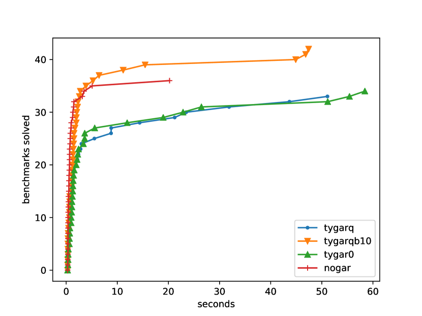
Figure 12. Queries solved over time for our initial variants and the best refinement bound.

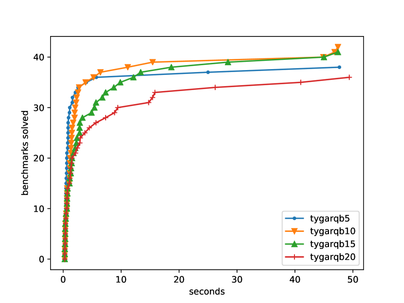
Figure 13. Queries solved over time for varying refinement bounds. The variant’s number indicates the refinement bound on the abstract cover.

We observe that NOGAR and TYGAR-Q have complimentary strengths and weaknesses: although NOGAR is usually faster, TYGAR-Q was able to find some solutions that NOGAR could not (for example, query 33: appBoth). We conclude that refinement is able to discover interesting abstractions, but because it is forced to make a new distinction between types in every iteration, after a while it is bound to start making irrelevant distinctions, and the ATN grows too large for the solver to efficiently navigate. To combine the strengths of the two approaches, we consider TYGAR-QB, which first uses refinement, and then switches to enumeration once the ATN reaches a certain bound on its number of places. To determine the optimal bound, we run the experiment with bounds 5, 10, 15, and 20.

Fig. 13 plots the results. As you can see, for easy queries, a bound of 5 performs the best: this correspond to our intuition that when the solution is easily reachable, it is faster to simply enumerate more candidates than spend time on refinement. However, as benchmarks get harder, having more places at ones disposal renders searches faster: the bounds of 10 and 15 seem to offer a sweet spot. Our best variant—TYGAR-QB $[10]$—solves 43 out of 44 queries with the median synthesis time of 1.4 seconds; in the rest of this section we use TYGAR-QB $[10]$ as the default H+ configuration.

TYGAR-QB $[10]$ solves all queries that were solved by NOGAR plus six additional queries on which NOGAR times out. A closer look at these six queries indicates that they tend to be more complex. For example, recall that NOGAR times out on the query appBoth, while TYGAR-QB $[10]$ finds a solution of size four in two seconds. Generally, our benchmark set is favorable for NOGAR: most Hoogle queries are easy, both because of programmers’ expectations of what Hoogle can do and also because we do not know the desired solution, and hence consider any (relevantly) well-typed solution correct. The benefits of refinement are more pronounced on queries with solution size four and higher: TYGAR-QB $[10]$ solves 6 out of 7, while NOGAR solves only 2.

6.2. Quality of Solutions

Setup. To evaluate the quality of the solutions, we ask H+ to return, for each query, at most five well-typed results within a timeout of 100 seconds. Complete results are available in Appendix B. We then manually inspect the solutions and for each one determine whether it is interesting, i.e. whether it is something a programmer might find useful, based on our own experience as Haskell programmers. Fig. 11 reports for each query, the number of interesting solutions, divided by the number of total solutions found within the timeout. To evaluate the effects of relevant typing and demand analysis (Sec. 2.3), we compare three variants of H+: (1) H+with all features enabled, based on TYGAR-QB, labeled H+. (2) Our tool without the demand analyzer filter, labeled H-D. (3) Our tool with structural typing in place of the relevant typing, labeled H-R (in this variant, the SMT solver is free to choose any non-negative number of tokens to assign to each query argument).

Analysis. First of all, we observe that whenever an interesting solution was found by H-D or H-R, it was also found by H+, indicating that our filters are not overly conservative. We also observe that on easy queries—taking less than a second—demand analysis and relevant typing did little to help: if an interesting solution were found, then all three variants would find it and give it a high rank. However, on medium and hard queries—taking longer than a second—the demand analyzer and relevant typing helped promote interesting solutions higher in rank. Overall, 66/179 solutions produces by H+ were interesting (37%), compared with 65/189 for H-D (34%) and 26/199 for H-R (13%). As you can see, relevant typing is essential to ensure that interesting solutions even get to the top five, whereas demand analysis is more useful to reduce the total number of solutions the programmer has to sift through. This is not surprising, since relevant typing mainly filters out short programs while demand analysis is left to deal with longer ones. In our experience, demand analysis was most useful when queries involved types like Either a b, where one could produce a value of type a from a value of type b by constructing and destructing the Either. One final observation is that in benchmarks 14, 18, 33, and 35, H-R found fewer results in total that the other two versions; we attribute this to the SMT solver struggling with determining the appropriate token multiplicities for the initial marking.

Noteworthy solutions. We presented three illustrative solutions generated by H+ as examples throughout Sec. 2:

• a $\rightarrow$ [Maybe a] $\rightarrow$ a corresponds to benchmark 19 (fromFirstMaybes); the solution from Sec. 2 is generated at rank 18.

• (a $\rightarrow$ a) $\rightarrow$ a $\rightarrow$ Int $\rightarrow$ a corresponds to benchmark 11 (applyNTimes); the solution from Sec. 2 is generated at rank 10.

• Eq a => [(a,b)] $\rightarrow$ a $\rightarrow$ b corresponds to benchmark 18 (lookup); the solution from Sec. 2 is generated at rank 1.

H+ has also produced code snippets that surprised us: for example, on the query (a $\rightarrow$ b, a) $\rightarrow$ b, the authors’ intuition was to destruct the pair then apply the function. Instead H+ produces \x $\rightarrow$ uncurry ($) x or alternatively \x $\rightarrow$ uncurry id x, both of which, contrary to our intuition, are not only well-typed, but also are functionally equivalent to our intended solution. It was welcome to see a synthesis tool write more succinct code that its authors.

7. Related Work

Finally, we situate our work with other research into ways of synthesizing code that meets a given specification. For brevity, we restrict ourselves to the (considerable) literature that focuses on using types as specifications, and omit discussing methods that use e.g. input-output examples or tests (Gulwani, 2011; Katayama, 2012; Lee et al., 2018; Osera and Zdancewic, 2015), logical specifications (Srivastava et al., 2010; Galenson et al., 2014) or program sketches (Solar-Lezama, 2008).

API Search. Modern IDEs support various forms of code-completion, based on at the very least common prefixes of names (e.g. completing In into Integer or fo into foldl’) and so on. Many tools use type information to only return completions that are well-typed at the point of completion. This approach is generalized by search based tools like Hoogle (Mitchell, 2004) that search for type isomorphisms (Di Cosmo, 1993) to find functions that “match” a given type signature (query). The above can be viewed as returning single-component results, as opposed to our goal of searching for terms that combine components in order to satisfy a given type query.

Search using Statistical Models. Several groups have looked into using statistical methods to improve search-based code-completion. One approach is to analyze large code bases to precompute statistical models that can be used to predict the most likely sequences of method calls at a given point or that yield values of a given (first order) type (Raychev et al., 2014). It is possible to generalize the above to train probabilistic models (grammars) that generate the most likely programs that must contain certain properties like method names, types, or keywords (Murali et al., 2017). We conjecture that while the above methods are very useful for effectively searching for commonly occurring code snippets, they are less useful in functional languages, where higher-order components offer high degree of compositionality and lead to less code repetition.

Type Inhabitation. The work most directly related to ours are methods based on finding terms that inhabit a (query) type (Urzyczyn, 1997). One approach is to use the correspondence between types and logics, to reduce the inhabitation question to that of validity of a logical formula (encoding the type). A classic example is Djinn (Augusstson, 2005) which implements a decision procedure for intuitionistic propositional calculus (Dyckhoff and Pinto, 1998) to synthesize terms that have a given type. Recent work by Rehof et al. extends the notion of inhabitation to support object oriented frameworks whose components behaviors can be specified via intersection types (Heineman et al., 2016). However, both these approaches lack a relevancy requirement of its snippets, and hence return undesirable results. For example, when queried with a type a $\rightarrow$ [a], Djinn would yield a function that always returns the empty list. One way to avoid undesirable results is to use dependent or refinement types to capture the semantics of the desired terms more precisely. Synquid (Polikarpova et al., 2016) and Myth2 (Frankle et al., 2016) use different flavors of refinement types to synthesize recursive functions, while Agda (Norell, 2008) makes heavy use of proof search to enable type- or hole-driven development. However, unlike H+, methods based on classical proof search do not scale up to large component libraries.

Scalable Proof Search. One way to scale search is explored by (Perelman et al., 2012) which uses a very restricted form of inhabitation queries to synthesize local “auto-completion” terms corresponding to method names, parameters, field lookups and so on, but over massive component libraries (e.g. the .NET framework). In contrast, the InSynth system (Gvero et al., 2013) addresses the problem of scalability by extending proof search with a notion of succinctness that collapses types into equivalence classes, thereby abstracting the space over which proof search must be performed. Further, InSynth uses weights derived from empirical analysis of library usage to bias the search to more likely results. However, InSynth is limited to simple types i.e. does not support parametric polymorphism which is the focus of our work.

Graph Reachability. Our approach is directly inspired by methods that reduce the synthesis problem to some form of reachability. Prospector (Mandelin et al., 2005) is an early exemplar where the components are unary functions that take a single input. Consequently, the component library can be represented as a directed graph of edges between input and output types, and synthesis is reduced to finding a path from the query’s input type to its output type. SyPet (Feng et al., 2017), which forms the basis of our work, is a generalization of Prospector to account for general first-order functions which can take multiple inputs, thereby generalizing synthesis to reachability on Petri nets. The key contribution of our work is the notion of TYGAR that generalizes SyPet’s approach to polymorphic and higher-order components.

Counterexample-Guided Abstraction Refinement. While the notion of counterexample-guided abstraction refinement (CEGAR) is classical at this point (Clarke et al., 2010), there are two lines of work in particular closely related to ours. First, (Ganty et al., 2007; Kloos et al., 2013) describe an iterative abstraction-refinement process for verifying Petri nets, using SMT (Esparza et al., 2014). However, in their setting, the refinement loop is used to perform unbounded verification of the (infinite-state) Petri net. In contrast, H+ performs a bounded search on each Petri net, but uses TYGAR to refine the net itself with new type instantiations that eliminate the construction of ill-typed terms. Second, Blaze (Wang et al., 2018) describes a CEGAR approach for synthesizing programs from input-output examples, by iteratively refining finite tree-automata whose states correspond to values in a predicate-abstraction domain. Programs that do not satisfy the input-output tests are used to iteratively refine the domain until a suitable correct program is found. Our approach differs in that we aim to synthesize terms of a given type. Consequently, although our refinement mechanism is inspired by Blaze, we develop a novel abstract domain—a finite sub-lattice of the type subsumption lattice—and show how to use proofs of untypeability to refine this domain. Moreover, we show how CEGAR can be combined with Petri nets (as opposed to tree automata) in order to enforce relevancy.

Types and Abstract Interpretation. The connection between types and abstract interpretation (AI) was first introduced in (Cousot, 1997). The goal of their work, however, was to cast existing type systems in the framework of AI, while we use this framework to systematically construct new type systems that further abstract an existing one. More recently, (Garcia et al., 2016) used the AI framework to formalize gradual typing. Like that work, we use AI to derive an abstract type system for our language, but otherwise the goals of the two techniques are very different. Moreover, as we hint in Sec. 4.3, our abstract domain is subtly but crucially different from traditional gradual typing, because our refinement algorithm relies on non-linear terms (i.e. types with repeated variables).

8. Conclusions

We have presented TYGAR, a new algorithm for synthesizing terms over polymorphic components that inhabit a given query type. The key challenge here is the infinite space of monomorphic instances arising from the polymorphic signatures. We introduced a new notion of abstract typing that allows us to use ideas from the framework of abstract interpretation to compute a finite overapproximation of this search space. We then show how spurious terms that are well-typed in the abstract domain but ill-typed in reality, yield proofs of untypeability which can then iteratively refine the abstract search space until a well-typed solution is found.

We have implemented TYGAR in H+, and our evaluation on a suite of 44 queries demonstrates the benefits of counterexample-driven refinement. In particular, we show how lazily refining a coarse abstract domain using proofs of untypeability allows us to synthesize correct results faster than a naive approach that eagerly instantiates all the types from the query followed by a brute-force enumeration. Our experiments further demonstrate that the gains from iterative refinement over enumeration are even more pronounced on harder queries over more complex types. Our support for polymorphism also allows H+ to work with higher-order and type-class constrained components, which, thanks to parametricity, allows for more precise queries than simple monomorphic types.

In future work it would be valuable to investigate ways to improve the quality of the results, e.g. by prioritizing components that are more popular, or less partial, or by extending our method to use other forms of specifications such as examples or refinement types.

Appendix A Proofs

A.1. Type Transformers

Lemma A.1 (Monotonicity of Substitution).

If $\sigma^{\prime}\sqsubseteq\sigma$ then ${\sigma^{\prime}}{B}\sqsubseteq{\sigma}{B}$.

Lemma A.2 (Monotonicity of Unification).

If $B_{1}\sqsubseteq B_{2}$ then $\mathsf{mgu}(B,B_{1})\sqsubseteq\mathsf{mgu}(B,B_{2})$

Lemma A.3 (Monotonicity of Type Transformers).

For any component $c$ and any types $\overline{B^{1}_{i}}$ and $\overline{B^{2}_{i}}$, such that $\overline{B^{1}_{i}\sqsubseteq B^{2}_{i}}$, we have $\llbracket c\rrbracket(\overline{B^{1}_{i}})\sqsubseteq\llbracket c\rrbracket(\overline{B^{2}_{i}})$.

Proof.

Let $\mathsf{fresh}(\Lambda(c))=\overline{B_{i}}\to B$. By the definition of type transformers, we have

$$\llbracket c\rrbracket(\overline{B^{1}_{i}}) ={\sigma_{1}}{B} \sigma_{1}=\mathsf{mgu}(\overline{B_{i},B^{1}_{i}})$$

$$\llbracket c\rrbracket(\overline{B^{2}_{i}}) ={\sigma_{2}}{B} \sigma_{2}=\mathsf{mgu}(\overline{B_{i},B^{2}_{i}})$$

Since $\overline{B^{1}_{i}\sqsubseteq B^{2}_{i}}$, we have $\sigma_{1}\sqsubseteq\sigma_{2}$ by A.2, and hence ${\sigma_{1}}{B}\sqsubseteq{\sigma_{2}}{B}$ by A.1. ∎

Lemma A.4 (Soundness of Type Transformers).

If $\mathsf{fresh}(\Lambda(c))=\overline{B_{i}}\to B$ and $\overline{{\sigma}{B_{i}}\sqsubseteq B^{\prime}_{i}}$ then ${\sigma}{B}\sqsubseteq\llbracket c\rrbracket(\overline{B^{\prime}_{i}})$.

Proof.

By A.3, since $\overline{{\sigma}{B_{i}}\sqsubseteq B^{\prime}_{i}}$, we have $\llbracket c\rrbracket(\overline{{\sigma}{B_{i}}})\sqsubseteq\llbracket c\rrbracket(\overline{B^{\prime}_{i}})$. But $\llbracket c\rrbracket(\overline{{\sigma}{B_{i}}})={\sigma}{B}$, because $\mathsf{mgu}(B,{\sigma}{B})\equiv\sigma$. Hence ${\sigma}{B}\sqsubseteq\llbracket c\rrbracket(\overline{B^{\prime}_{i}})$ as desired. ∎

A.2. Algorithmic Typing

Typing $\boxed{\Lambda;\Gamma\vdash E::t}$

$$\inference[\textsc{T-Var}]{\Gamma(x)=b}{\Lambda;\Gamma\vdash x::b}$$

$$\inference[\textsc{T-Fun}]{\Lambda;\Gamma,x:b\vdash E::t}{\Lambda;\Gamma\vdash\lambda{x}.{E}::b\to t}$$

Figure 14. Uncurried version of declarative typing.

In the following, we use a version the declarative type system in Sec. A.2, which is defined over uncurried applications, and hence more closely matches algorithmic typing. It is straightforward to show that for terms in $\eta$-long form, this type system is equivalent to the one in Sec. 3.1.

Lemma A.5 (Soundness of inference).

If $\Lambda;\Gamma\vdash e\Longrightarrow B$ and $b\sqsubseteq B$, then $\Lambda;\Gamma\vdash e::b$.

Proof.

By induction on the derivation of $\Lambda;\Gamma\vdash e\Longrightarrow B$.

• Case I-Var: Given the conclusion $\Lambda;\Gamma\vdash x\Longrightarrow b^{\prime}$, we get to assume $\Gamma(x)=b^{\prime}$. Consequently, applying T-Var, we get $\Lambda;\Gamma\vdash x::b^{\prime}$. But since $b^{\prime}$ is ground and $b\sqsubseteq b^{\prime}$, we have $b^{\prime}=b$.

• Case I-App: Given the conclusion $\Lambda;\Gamma\vdash{c}\ {\overline{e_{i}}}\Longrightarrow\llbracket c\rrbracket(\overline{B_{i}})$, we get to assume $\overline{\Lambda;\Gamma\vdash e_{i}\Longrightarrow B_{i}}$. Assume $\mathsf{fresh}(\Lambda(c))=\overline{B^{\prime}_{i}}\to B^{\prime}$. By definition of $\llbracket c\rrbracket$ we have $\llbracket c\rrbracket(\overline{B_{i}})={\sigma_{1}}{B^{\prime}}$ where $\sigma_{1}=\mathsf{mgu}(\overline{B^{\prime}_{i},B_{i}})$. By the assumption of the theorem $b\sqsubseteq B=\llbracket c\rrbracket(\overline{B_{i}})$, and hence there exists $\sigma_{2}$ such that $b={\sigma_{2}}{(\llbracket c\rrbracket(\overline{B_{i}}))}={(\sigma_{2}\circ\sigma_{1})}{B^{\prime}}$.

  Let $\rho$ be some substitution such that ${(\rho\circ\sigma_{2}\circ\sigma_{1})}{B^{\prime}_{i}}$, is ground for all for all $B^{\prime}_{i}$; we will denote these ground types $b_{i}$. Then each $b_{i}={(\rho\circ\sigma_{2})}{({\sigma_{1}}{B^{\prime}_{i}})}={(\rho\circ\sigma_{2})}{({\sigma_{1}}{B_{i}})}$ (since $\sigma_{1}$ is a unifier), and hence $b_{i}\sqsubseteq B_{i}$. Then by the IH, we can show for all $e_{i}$: $\Lambda;\Gamma\vdash e_{i}::b_{i}$ (1).

  Finally, let us use T-App to construct the derivation of $\Lambda;\Gamma\vdash{c}\ {\overline{e_{i}}}::b$ The middle premise follows with $\sigma=\rho\circ\sigma_{2}\circ\sigma_{1}$ (note that ${\sigma}{B^{\prime}}={\rho}{b}=b$, since $b$ is already ground). We get the last premise by (1).

∎

Lemma A.6 (Completeness of Inference).

If $\Lambda;\Gamma\vdash e::b$, then $\exists B.\Lambda;\Gamma\vdash e\Longrightarrow B$ and $b\sqsubseteq B$.

Proof.

By induction on the derivation of $\Lambda;\Gamma\vdash e::b$.

• Case T-Var: Given the conclusion $\Lambda;\Gamma\vdash x::b$, we get to assume $\Gamma(x)=b$. Using I-Var we build the derivation $\Lambda;\Gamma\vdash x\Longrightarrow b$. Trivially $b\sqsubseteq b$ by reflexivity of $\sqsubseteq$.

• Case T-App: Given the conclusion $\Lambda;\Gamma\vdash{c}\ {\overline{e_{i}}}::b$, we get to assume for each $i$: $\Lambda;\Gamma\vdash e_{i}::b_{i}$, where $\overline{b_{i}}\to b={\sigma}{T}$ and $T=\overline{B^{\prime}_{i}}\to B^{\prime}=\mathsf{fresh}(\Lambda(c))$. By IH we obtain $\overline{B_{i}}$, such that $\Lambda;\Gamma\vdash e_{i}\Longrightarrow B_{i}$ and $b_{i}\sqsubseteq B_{i}$, for each $i$. Using I-Var we build the derivation $\Lambda;\Gamma\vdash{c}\ {\overline{e_{i}}}\Longrightarrow\llbracket c\rrbracket(\overline{B_{i}})$. It remains to show that $b\sqsubseteq\llbracket c\rrbracket(\overline{B_{i}})$.

  Since $\overline{b_{i}\sqsubseteq B_{i}}$ and $b_{i}={\sigma}{B^{\prime}_{i}}$, we get $\overline{{\sigma}{B^{\prime}_{i}}\sqsubseteq B_{i}}$. Hence we can apply A.4 to conclude ${\sigma}{B^{\prime}}\sqsubseteq\llbracket c\rrbracket(\overline{B_{i}})$, but ${\sigma}{B^{\prime}}=b$, so we obtain the desired conclusion.

• Case T-Fun: impossible since $b$ is a base type.

∎

Lemma A.7 (Soundness of Checking).

If $\Lambda;\Gamma\vdash E\Longleftarrow t$, then $\Lambda;\Gamma\vdash E::t$.

Proof.

By induction on the derivation of $\Lambda;\Gamma\vdash E\Longleftarrow t$.

• Case C-Base: Given the conclusion $\Lambda;\Gamma\vdash e\Longleftarrow b$, we get to assume $\Lambda;\Gamma\vdash e\Longrightarrow B$ and $b\sqsubseteq B$. By A.5, we directly obtain $\Lambda;\Gamma\vdash e::b$.

• Case C-Fun: Given the conclusion $\Lambda;\Gamma\vdash\lambda{x}.{E}\Longleftarrow b\to t$, we get to assume $\Lambda;\Gamma,x:b\vdash E\Longleftarrow t$. By IH, we get $\Lambda;\Gamma,x:b\vdash E::t$. Hence we use T-Fun to obtain $\Lambda;\Gamma\vdash\lambda{x}.{e}::b\to t$.

∎

Lemma A.8 (Completeness of Checking).

If $\Lambda;\Gamma\vdash E::t$ then $\Lambda;\Gamma\vdash E\Longleftarrow t$.

Proof.

By induction on the derivation of $\Lambda;\Gamma\vdash E::t$.

• Case T-Var, T-App: Given $\Lambda;\Gamma\vdash e::b$, we use A.6 to derive $\Lambda;\Gamma\vdash e\Longrightarrow B$ and $b\sqsubseteq B$. Hence we apply C-Base to obtain $\Lambda;\Gamma\vdash e\Longleftarrow b$.

• Case T-Fun: Given the conclusion $\Lambda;\Gamma\vdash\lambda{x}.{E}::b\to t$ we get to assume $\Lambda;\Gamma,x:b\vdash E::t$. By IH $\Lambda;\Gamma,x:b\vdash E\Longleftarrow t$. We apply C-Fun to obtain $\Lambda;\Gamma\vdash\lambda{x}.{e}\Longleftarrow b\to t$.

∎

Theorem A.9 (Type Checking is Sound and Complete).

$\Lambda;\cdot\vdash E::t$ iff $\Lambda;\cdot\vdash E\Longleftarrow t$.

Proof.

By A.7 and A.8. ∎

A.3. Abstract Typing

Lemma A.10 (Refinement).

If $B^{\prime}\sqsubseteq B$ and $\mathcal{A}^{\prime}\preceq\mathcal{A}$, then $\alpha_{\mathcal{A}^{\prime}}(B^{\prime})\sqsubseteq\alpha_{\mathcal{A}}(B)$.

Proof.

Let $A=\alpha_{\mathcal{A}}(B)$, $A^{\prime}=\alpha_{\mathcal{A}^{\prime}}(B^{\prime})$. Because $\mathcal{A}\subseteq\mathcal{A}^{\prime}$, we have $A\in\mathcal{A}^{\prime}$. Since $B^{\prime}\sqsubseteq B\sqsubseteq A$, we have $A^{\prime}\sqsubseteq A$ by definition of $\alpha_{\mathcal{A}^{\prime}}$. ∎

Lemma A.11 (Inference Refinement).

If $\mathcal{A}^{\prime}\preceq\mathcal{A}$ and $\Lambda;\Gamma\vdash_{\mathcal{A}^{\prime}}e\Longrightarrow B^{\prime}$, then $\Lambda;\Gamma\vdash_{\mathcal{A}}e\Longrightarrow B$ and $B^{\prime}\sqsubseteq B$.

Proof.

By induction on the derivation of $\Lambda;\Gamma\vdash_{\mathcal{A}^{\prime}}e\Longrightarrow B^{\prime}$.

• Case I-Var: Follows by A.10.

• Case I-App: Given the conclusion $\Lambda;\Gamma\vdash_{\mathcal{A}^{\prime}}{c}\ {\overline{e_{i}}}\Longrightarrow\alpha_{\mathcal{A}^{\prime}}\left(\llbracket c\rrbracket(\overline{B^{\prime}_{i}})\right)$, we get to assume $\Lambda;\Gamma\vdash_{\mathcal{A}^{\prime}}e_{i}\Longrightarrow B^{\prime}_{i}$ for all $i$. By IH we get $\Lambda;\Gamma\vdash_{\mathcal{A}}e_{i}\Longrightarrow B_{i}$ and $B^{\prime}_{i}\sqsubseteq B_{i}$. We use I-App to obtain $\Lambda;\Gamma\vdash_{\mathcal{A}}{c}\ {\overline{e_{i}}}\Longrightarrow\alpha_{\mathcal{A}}\left(\llbracket c\rrbracket(\overline{B_{i}})\right)$. Furthermore, by A.3, we get $\llbracket c\rrbracket(\overline{B^{\prime}_{i}})\sqsubseteq\llbracket c\rrbracket(\overline{B_{i}})$, and hence by A.10, $\alpha_{\mathcal{A}^{\prime}}\left(\llbracket c\rrbracket(\overline{B^{\prime}_{i}})\right)\sqsubseteq\alpha_{\mathcal{A}}\left(\llbracket c\rrbracket(\overline{B_{i}})\right)$.

∎

Theorem A.12 (Typing Preservation).

If $\mathcal{A}^{\prime}\preceq\mathcal{A}$ and $\Lambda;\Gamma\vdash_{\mathcal{A}^{\prime}}E\Longleftarrow t$ then $\Lambda;\Gamma\vdash_{\mathcal{A}}E\Longleftarrow t$.

Proof.

By induction on the derivation of $\Lambda;\Gamma\vdash_{\mathcal{A}^{\prime}}E\Longleftarrow t$.

• Case C-Base: Given the conclusion $\Lambda;\Gamma\vdash_{\mathcal{A}^{\prime}}e\Longleftarrow b$, we get to assume $\Lambda;\Gamma\vdash_{\mathcal{A}^{\prime}}e\Longrightarrow B^{\prime}$ and $b\sqsubseteq B^{\prime}$. Then by A.11 we get $\Lambda;\Gamma\vdash_{\mathcal{A}}e\Longrightarrow B$ and $B^{\prime}\sqsubseteq B$, hence $b\sqsubseteq B$. We use C-Base to conclude $\Lambda;\Gamma\vdash_{\mathcal{A}}e\Longleftarrow b$.

• Case C-Fun: Given the conclusion $\Lambda;\Gamma\vdash_{\mathcal{A}^{\prime}}\lambda{x}.{E}\Longleftarrow b\to t$ we get to assume $\Lambda;\Gamma,x:b\vdash_{\mathcal{A}^{\prime}}E\Longleftarrow t$. By IH we get $\Lambda;\Gamma,x:b\vdash_{\mathcal{A}}E\Longleftarrow t$. We use C-Fun to colclude $\Lambda;\Gamma\vdash_{\mathcal{A}}\lambda{x}.{E}\Longleftarrow b\to t$.

∎

A.4. Synthesis

Theorem A.13.

The synthesis problem in $\lambda_{H}$ is undecidable.

Proof.

By reduction from the Post Correspondence Problem (PCP). Let $[(a_{1},b_{1}),\ldots,(a_{n},b_{n})]$ be an instance of the PCP, where each $a_{i}$, $b_{i}$ are bit strings. We translate this instance into a synthesis problem $(\Lambda,T)$ as follows.

The set of type constructors in $\Lambda$ is: two nullary constructors Start and Goal, two unary constructors T and F, and a single binary constructor P. Given a bit string $bs$ and a type $T$, the type $\mathsf{wrap}(T,bs)$ is defined as follows:

$$\mathsf{wrap}(T,[]) =T$$

$$\mathsf{wrap}(T,0:bs) {\displaystyle=\mathsf{wrap}(\mbox{\leavevmode\lstinline{{\lst@@@set@language\lst@@@set@numbers\lst@@@set@frame\lst@@@set@rulecolor\lst@@@set@language\lst@@@set@numbers\lst@@@set@language{\@listingGroup{ltx_lst_identifier}{F}}}}}}\ T,bs)$$

$$\mathsf{wrap}(T,1:bs) {\displaystyle=\mathsf{wrap}(\mbox{\leavevmode\lstinline{{\lst@@@set@language\lst@@@set@numbers\lst@@@set@frame\lst@@@set@rulecolor\lst@@@set@language\lst@@@set@numbers\lst@@@set@language{\@listingGroup{ltx_lst_identifier}{T}}}}}}\ T,bs)$$

Now we can define the set of components in $\Lambda$:

• for each pair $(a_{i},b_{i})$, there is a component $s_{i}$ of type ${{{{\mbox{\leavevmode\lstinline{{\lst@@@set@language\lst@@@set@numbers\lst@@@set@frame\lst@@@set@rulecolor\lst@@@set@language\lst@@@set@numbers\lst@@@set@language{\@listingGroup{ltx_lst_identifier}{Start}}}}}}\to\mbox{\leavevmode\lstinline{{\lst@@@set@language\lst@@@set@numbers\lst@@@set@frame\lst@@@set@rulecolor\lst@@@set@language\lst@@@set@numbers\lst@@@set@language{\@listingGroup{ltx_lst_identifier}{P}}}}}}\ \mathsf{wrap}(\mbox{\leavevmode\lstinline{{\lst@@@set@language\lst@@@set@numbers\lst@@@set@frame\lst@@@set@rulecolor\lst@@@set@language\lst@@@set@numbers\lst@@@set@language{\@listingGroup{ltx_lst_identifier}{Start}}}}}},a_{i})\ \mathsf{wrap}(\mbox{\leavevmode\lstinline{{\lst@@@set@language\lst@@@set@numbers\lst@@@set@frame\lst@@@set@rulecolor\lst@@@set@language\lst@@@set@numbers\lst@@@set@language{\@listingGroup{ltx_lst_identifier}{Start}}}}}},b_{i})$;

• for each pair $(a_{i},b_{i})$, there is a component $n_{i}$ of type ${{\forall\alpha\beta.\mbox{\leavevmode\lstinline{{\lst@@@set@language\lst@@@set@numbers\lst@@@set@frame\lst@@@set@rulecolor\lst@@@set@language\lst@@@set@numbers\lst@@@set@language{\@listingGroup{ltx_lst_identifier}{P}}}}}}\ \alpha\ \beta\to\mbox{\leavevmode\lstinline{{\lst@@@set@language\lst@@@set@numbers\lst@@@set@frame\lst@@@set@rulecolor\lst@@@set@language\lst@@@set@numbers\lst@@@set@language{\@listingGroup{ltx_lst_identifier}{P}}}}}}\ \mathsf{wrap}(\alpha,a_{i})\ \mathsf{wrap}(\beta,b_{i})$;

• a component $f$ of type ${{\forall\alpha.\mbox{\leavevmode\lstinline{{\lst@@@set@language\lst@@@set@numbers\lst@@@set@frame\lst@@@set@rulecolor\lst@@@set@language\lst@@@set@numbers\lst@@@set@language{\@listingGroup{ltx_lst_identifier}{P}}}}}}\ \alpha\ \alpha\to\mbox{\leavevmode\lstinline{{\lst@@@set@language\lst@@@set@numbers\lst@@@set@frame\lst@@@set@rulecolor\lst@@@set@language\lst@@@set@numbers\lst@@@set@language{\@listingGroup{ltx_lst_identifier}{Goal}}}}}}$.

The query type $T$ is ${{\mbox{\leavevmode\lstinline{{\lst@@@set@language\lst@@@set@numbers\lst@@@set@frame\lst@@@set@rulecolor\lst@@@set@language\lst@@@set@numbers\lst@@@set@language{\@listingGroup{ltx_lst_identifier}{Start}}}}}}\to\mbox{\leavevmode\lstinline{{\lst@@@set@language\lst@@@set@numbers\lst@@@set@frame\lst@@@set@rulecolor\lst@@@set@language\lst@@@set@numbers\lst@@@set@language{\@listingGroup{ltx_lst_identifier}{Goal}}}}}}$. The sequence of P instances in the solution to this synthesis problem corresponds to the solution to the PCP. ∎

For example, a PCP instance $[(1,101),(10,00),(011,11)]$ gives rise to the following components:

⬇

s1 :: Start $\rightarrow$ P (T Start) (T (F (T Start)))

s2 :: Start $\rightarrow$ P (F (T Start)) (F (F Start))

s3 :: Start $\rightarrow$ P (T (T (F Start))) (T (T Start))

n1 :: P $\alpha$ $\beta$ $\rightarrow$ P (T $\alpha$) (T (F (T $\beta$)))

n2 :: P $\alpha$ $\beta$ $\rightarrow$ P (F (T $\alpha$)) (F (F $\beta$))

n3 :: P $\alpha$ $\beta$ $\rightarrow$ P (T (T (F $\alpha$))) (T (T $\beta$))

f :: P $\alpha$ $\alpha$ $\rightarrow$ Goal

The solution for this instance is \x $\rightarrow$ f (n3 (n2 (n3 (s1 x)))).

A.5. Proof of Untypeability

For a $P\colon\mathbf{e}\to\mathbf{B_{\bot}}$ and a term $e^{*}$, define

$\mathcal{I}_{1}$::

For any $e\in\mathsf{subterms}(e^{*})$, if $\Lambda;\Gamma\vdash e\Longrightarrow B$, then $B\sqsubseteq P[e]$;

$\mathcal{I}_{2}$::

For any $e={c}\ {\overline{e_{j}}}\in\mathsf{subterms}(e^{*})$, $\llbracket c\rrbracket(\overline{P[e_{j}]})\sqsubseteq P[e]$;

$\mathcal{I}_{3}$::

$P[e^{*}]=\bot$.

Lemma A.14 (Precision of Inference).

If $\mathcal{I}_{1}\wedge\mathcal{I}_{2}$, $\mathsf{range}(P)\subseteq\mathcal{A}$, $e\in\mathsf{subterms}(e^{*})$, and $\Lambda;\Gamma\vdash_{\mathcal{A}}e\Longrightarrow B$, then $B\sqsubseteq P[e]$.

Proof.

By induction on the derivation of $\Lambda;\Gamma\vdash_{\mathcal{A}}e\Longrightarrow B$.

• Case I-Var: Given the conclusion $\Lambda;\Gamma\vdash_{\mathcal{A}}x\Longrightarrow\alpha_{\mathcal{A}}(b)$, we get to assume $\Gamma(x)=b$, and hence $\Lambda;\Gamma\vdash x\Longrightarrow b$. By $\mathcal{I}_{1}$, we have $b\sqsubseteq P[x]$.

• Case I-App: Given the conclusion $\Lambda;\Gamma\vdash_{\mathcal{A}}{c}\ {\overline{e_{i}}}\Longrightarrow\alpha_{\mathcal{A}}(\llbracket c\rrbracket(\overline{B_{i}}))$, we get to assume $\Lambda;\Gamma\vdash_{\mathcal{A}}e_{i}\Longrightarrow B_{i}$ for each $i$. By IH, we have $B_{i}\sqsubseteq P[e_{i}]$ for each $i$. Then by A.3 we have $\llbracket c\rrbracket(\overline{B_{i}})\sqsubseteq\llbracket c\rrbracket(\overline{P[e_{i}]})$, and by $\mathcal{I}_{2}$ we have $\llbracket c\rrbracket(\overline{P[e_{i}]})\sqsubseteq P[e]$; hence $\llbracket c\rrbracket(\overline{B_{i}})\sqsubseteq P[e]$. Applying $\alpha_{\mathcal{A}}$ to both sides, by A.10 we have $\alpha_{\mathcal{A}}(\llbracket c\rrbracket(\overline{B_{i}}))\sqsubseteq\alpha_{\mathcal{A}}(P[e])$. But $\alpha_{\mathcal{A}}(P[e])=P[e]$ because $\mathsf{range}(P)\subseteq\mathcal{A}$, hence we get $\alpha_{\mathcal{A}}(\llbracket c\rrbracket(\overline{B_{i}}))\sqsubseteq P[e]$ as required.

∎

Lemma A.15 (Untypeability).

Let $E=\lambda{\overline{x_{i}}}.{e}$, $t=\overline{b_{i}}\to b$, $e^{*}={r}\ {e}$, where $\Lambda(r)=b\to b$. If $\mathcal{I}_{1}\wedge\mathcal{I}_{2}\wedge\mathcal{I}_{3}$ and $\mathsf{range}(P)\subseteq\mathcal{A}$, then $\Lambda;\cdot\not\vdash_{\mathcal{A}}E\Longleftarrow t$.

Proof.

Assume the contrary: that we can derive $\Lambda;\cdot\vdash_{\mathcal{A}}E\Longleftarrow t$. Then we must be able to derive $\Lambda;\Gamma\vdash_{\mathcal{A}}e\Longleftarrow b$, where $\Gamma=\overline{x_{i}\colon b_{i}}$. By C-Base, if we derive $\Lambda;\Gamma\vdash_{\mathcal{A}}e\Longrightarrow B$, it must be that $b\sqsubseteq B$ (note that inference result always exists and is unique).

By A.14, $\Lambda;\Gamma\vdash_{\mathcal{A}}e^{*}\Longrightarrow B^{*}\sqsubseteq P[e^{*}]$, but by $\mathcal{I}_{3}$ we have $P[e^{*}]=\bot$, hence $B^{*}=\bot$. By I-App and considering $\Lambda(r)$, we have $B^{*}={\sigma}{b}$, where $\sigma=\mathsf{mgu}(B,b)$. The only $\sigma$ such that ${\sigma}{b}=\bot$ is $\sigma_{\bot}$, hence we get $\mathsf{mgu}(B,b)=\sigma_{\bot}$. But then it cannot be that $b\sqsubseteq B$, a contradiction. ∎

Appendix B Evaluation Results

appBoth: (a $\rightarrow$ b) $\rightarrow$ (a $\rightarrow$ c) $\rightarrow$ a $\rightarrow$ (b, c)
Demand Analysis (,) (arg2 arg0) (arg1 arg0) (,) (($) arg2 arg0) (arg1 arg0) (,) (arg2 (fromJust Nothing)) (arg1 arg0) (,) (arg2 (head [])) (arg1 arg0) (,) (arg2 (last [])) (arg1 arg0)
No Demand Analysis (,) (arg2 arg0) (arg1 arg0) (,) (($) arg2 arg0) (arg1 arg0) (,) (arg2 (fromJust Nothing)) (arg1 arg0) (,) (arg2 (head [])) (arg1 arg0) (,) (arg2 (last [])) (arg1 arg0)
No Relevancy (,) (arg2 arg0) (arg1 arg0)
countFilter: (a $\rightarrow$ Bool) $\rightarrow$ [a] $\rightarrow$ Int
Demand Analysis length (map arg1 arg0) length (dropWhile arg1 arg0) length (filter arg1 arg0) length (takeWhile arg1 arg0) length (repeat (arg1 (head arg0)))
No Demand Analysis length (map arg1 arg0) length (dropWhile arg1 arg0) length (filter arg1 arg0) length (takeWhile arg1 arg0) length (repeat (arg1 (head arg0)))
No Relevancy length (map arg1 arg0) length (dropWhile arg1 arg0) length (filter arg1 arg0) length (takeWhile arg1 arg0) length (repeat arg1)
mbElem: Eq a => a $\rightarrow$ [a] $\rightarrow$ Maybe a
Demand Analysis lookup arg1 (zip arg0 []) lookup arg1 (zip [] arg0) lookup arg1 (zip arg0 arg0)
No Demand Analysis lookup arg1 (zip arg0 []) lookup arg1 (zip [] arg0) lookup arg1 (zip arg0 arg0)
No Relevancy Just arg1 listToMaybe arg0 Nothing listToMaybe (cycle arg0) listToMaybe (init arg0)
hoogle01: (a $\rightarrow$ b) $\rightarrow$ [a] $\rightarrow$ b
Demand Analysis arg1 (head arg0) arg1 (last arg0) ($) arg1 (head arg0) ($) arg1 (last arg0) arg1 (head (cycle arg0))
No Demand Analysis arg1 (head arg0) arg1 (last arg0) ($) arg1 (head arg0) ($) arg1 (last arg0) arg1 (head (cycle arg0))
No Relevancy arg1 (head arg0) arg1 (last arg0) arg1 (fromJust (listToMaybe arg0)) arg1 (fromJust Nothing) ($) arg1 (head arg0)
fromFirstMaybes: a $\rightarrow$ [Maybe a] $\rightarrow$ a
Demand Analysis fromMaybe arg1 (head arg0) fromMaybe arg1 (last arg0) maybe arg1 id (head arg0) maybe arg1 id (last arg0) bool arg1 arg1 (null arg0)
No Demand Analysis fromRight arg1 (Left arg0) fromLeft arg1 (Right arg0) fromMaybe arg1 (head arg0) fromMaybe arg1 (last arg0) fromLeft arg1 (Right (catMaybes arg0))
No Relevancy fromLeft arg1 (Right arg0) fromRight arg1 (Left arg0) fromLeft arg1 (Right arg1) fromRight arg1 (Right arg1) fromLeft arg1 (Left arg1)
mbAppFirst: b $\rightarrow$ (a $\rightarrow$ b) $\rightarrow$ [a] $\rightarrow$ b
Demand Analysis maybe arg2 arg1 (listToMaybe arg0) fromMaybe arg2 (listToMaybe (map arg1 arg0)) fromLeft arg2 (Right (arg1 (head arg0)))
No Demand Analysis maybe arg2 arg1 (listToMaybe arg0) fromLeft (arg1 (head arg0)) (Right arg2) fromRight (arg1 (head arg0)) (Right arg2) fromLeft (arg1 (head arg0)) (Left arg2) fromRight (arg1 (head arg0)) (Left arg2)
No Relevancy arg1 (head arg0) arg1 (last arg0) fromLeft arg2 (Right arg1) fromRight arg2 (Left arg1) ($) arg1 (head arg0)
appendN: Int $\rightarrow$ [a] $\rightarrow$ [a]
Demand Analysis drop arg1 arg0 take arg1 arg0 drop arg1 (cycle arg0) take arg1 (cycle arg0) drop arg1 (init arg0)
No Demand Analysis drop arg1 arg0 take arg1 arg0 drop arg1 (cycle arg0) take arg1 (cycle arg0) drop arg1 (init arg0)
No Relevancy cycle arg0 init arg0 reverse arg0 tail arg0 drop arg1 arg0
firstMaybe: [Maybe a] $\rightarrow$ a
Demand Analysis fromJust (head arg0) fromJust (last arg0) head (catMaybes arg0) last (catMaybes arg0) fromJust (head (cycle arg0))
No Demand Analysis fromJust (head arg0) fromJust (last arg0) head (catMaybes arg0) last (catMaybes arg0) fromJust (head (cycle arg0))
No Relevancy head [] last [] fromJust (head arg0) fromJust (last arg0) fromJust Nothing
mapEither: (a $\rightarrow$ Either b c) $\rightarrow$ [a] $\rightarrow$ ([b], [c])
Demand Analysis partitionEithers (map arg1 arg0) partitionEithers (repeat (arg1 (head arg0))) partitionEithers (repeat (arg1 (last arg0))) curry (last []) arg1 arg0
No Demand Analysis partitionEithers (map arg1 arg0) partitionEithers (repeat (arg1 (head arg0))) partitionEithers (repeat (arg1 (last arg0))) curry (head []) arg1 arg0 curry (last []) arg1 arg0
No Relevancy partitionEithers (map arg1 arg0)
head-rest: [a] $\rightarrow$ (a, [a])
Demand Analysis fromJust (uncons arg0) (,) (last arg0) arg0 (,) (head arg0) arg0 (,) (last arg0) [] (,) (head arg0) []
No Demand Analysis fromJust (uncons arg0) (,) (last arg0) arg0 (,) (head arg0) arg0 (,) (last arg0) [] (,) (head arg0) []
No Relevancy head [] last [] fromJust (uncons arg0) fromJust Nothing (,) (head arg0) arg0
applyPair: (a $\rightarrow$ b, a) $\rightarrow$ b
Demand Analysis uncurry ($) arg0 uncurry id arg0 ($) (fst arg0) (snd arg0)
No Demand Analysis uncurry ($) arg0 uncurry id arg0 ($) (fst arg0) (snd arg0) uncurry (head []) arg0 ($) (head []) arg0
No Relevancy uncurry id arg0 uncurry ($) arg0 fromJust Nothing head [] last []
maybe: Maybe a $\rightarrow$ a $\rightarrow$ Maybe a
Demand Analysis Just (fromMaybe arg0 arg1) Just (maybe arg0 id arg1) listToMaybe (repeat (fromMaybe arg0 arg1)) curry (last []) arg1 arg0 curry (last []) arg0 arg1
No Demand Analysis Just (fromMaybe arg0 arg1) fromRight arg1 (Left arg0) fromLeft arg1 (Right arg0) fromRight (Just arg0) (Left arg1) fromLeft (Just arg0) (Left arg1)
No Relevancy Just arg0 Nothing fromRight arg1 (Left arg0) fromLeft arg1 (Right arg0) ($) id arg1
multiAppPair: (a $\rightarrow$ b, a $\rightarrow$ c) $\rightarrow$ a $\rightarrow$ (b, c)
Demand Analysis (,) (($) (fst arg1) arg0) (($) (snd arg1) arg0) curry (last []) arg0 arg1
No Demand Analysis (,) (($) (fst arg1) arg0) (($) (snd arg1) arg0) curry (fromJust Nothing) arg0 arg1 curry (head []) arg0 arg1 curry (last []) arg0 arg1
No Relevancy fromJust Nothing head [] last []
applyNtimes: (a $\rightarrow$ a) $\rightarrow$ a $\rightarrow$ Int $\rightarrow$ a
Demand Analysis arg2 ((!!) (repeat arg1) arg0) arg2 (head (replicate arg0 arg1)) arg2 (last (replicate arg0 arg1)) head (replicate arg0 (arg2 arg1)) last (replicate arg0 (arg2 arg1))
No Demand Analysis arg2 (fromRight arg1 (Left arg0)) arg2 (fromLeft arg1 (Right arg0)) fromRight (arg2 arg1) (Left arg0) fromLeft (arg2 arg1) (Right arg0) arg2 ((!!) (repeat arg1) arg0)
No Relevancy arg2 arg1 arg2 (arg2 arg1) ($) arg2 arg1 fromMaybe (arg2 arg1) (Just (arg2 arg1)) fromMaybe (arg2 arg1) Nothing
splitAtFirst: a $\rightarrow$ [a] $\rightarrow$ ([a], [a])
Demand Analysis (,) arg0 (repeat arg1) swap ((,) arg0 (repeat arg1)) splitAt (length arg0) (repeat arg1) (,) (repeat arg1) (cycle arg0) (,) (repeat arg1) (init arg0)
No Demand Analysis (,) arg0 (repeat arg1) swap ((,) arg0 (repeat arg1)) splitAt (length arg0) (repeat arg1) (,) (repeat arg1) (cycle arg0) (,) (repeat arg1) (init arg0)
No Relevancy (,) arg0 arg0 (,) (cycle arg0) (cycle arg0) (,) (init arg0) (init arg0) (,) (reverse arg0) (reverse arg0) (,) (tail arg0) (tail arg0)
eitherTriple: Either a b $\rightarrow$ Either a b $\rightarrow$ Either a b
Demand Analysis bool arg1 arg1 (isRight arg0) bool arg1 arg1 (isLeft arg0) fromMaybe arg1 (listToMaybe (repeat arg0)) bool arg1 arg0 (last []) bool arg1 arg0 (and [])
No Demand Analysis fromLeft arg1 (Left arg0) fromRight arg1 (Left arg0) bool arg1 arg0 False bool arg1 arg0 True bool arg1 arg0 otherwise
No Relevancy fromMaybe arg1 Nothing bool arg1 arg1 False bool arg1 arg1 True bool arg1 arg1 otherwise fromLeft arg1 (Right arg1)
multiApp: (a $\rightarrow$ b $\rightarrow$ c) $\rightarrow$ (a $\rightarrow$ b) $\rightarrow$ a $\rightarrow$ c
Demand Analysis arg2 arg0 (arg1 arg0) arg2 (fromJust Nothing) (arg1 arg0) arg2 (head []) (arg1 arg0) arg2 (last []) (arg1 arg0) arg2 arg0 (arg1 (fromJust Nothing))
No Demand Analysis arg2 arg0 (arg1 arg0) arg2 arg0 (($) arg1 arg0) arg2 (fromJust Nothing) (arg1 arg0) arg2 (head []) (arg1 arg0) arg2 (last []) (arg1 arg0)
No Relevancy arg2 arg0 (arg1 arg0) arg2 arg0 (($) arg1 arg0) arg2 (snd ((,) (arg1 arg0) arg0)) (fst ((,) (arg1 arg0) arg0)) uncurry arg2 ((,) arg0 (arg1 arg0)) arg2 (snd ((,) arg0 arg0)) (arg1 (fst ((,) arg0 arg0)))
mergeEither: Either a (Either a b) $\rightarrow$ Either a b
Demand Analysis fromRight (fromJust Nothing) arg0 fromRight (head []) arg0 fromRight (last []) arg0
No Demand Analysis fromRight (fromJust Nothing) arg0 fromRight (head []) arg0 fromRight (last []) arg0
No Relevancy fromJust Nothing head [] last [] fromRight (fromJust Nothing) arg0 fromRight (head []) arg0
firstRight: [Either a b] $\rightarrow$ Either a b
Demand Analysis head arg0 last arg0 head (cycle arg0) last (cycle arg0) head (init arg0)
No Demand Analysis head arg0 last arg0 head (cycle arg0) last (cycle arg0) head (init arg0)
No Relevancy head arg0 last arg0 head (cycle arg0) last (cycle arg0) head (init arg0)
flatten: [[[a]]] $\rightarrow$ [a]
Demand Analysis head (head arg0) last (head arg0) concat (head arg0) head (last arg0) last (last arg0)
No Demand Analysis head (head arg0) last (head arg0) concat (head arg0) head (last arg0) last (last arg0)
No Relevancy [] lefts [] rights [] catMaybes [] cycle []
pipe: [(a $\rightarrow$ a)] $\rightarrow$ (a $\rightarrow$ a)
Demand Analysis foldr ($) arg0 arg1 ($) (head arg1) arg0 ($) (last arg1) arg0 foldr id arg0 arg1 foldr id arg0 (cycle arg1)
No Demand Analysis foldr ($) arg0 arg1 fromLeft arg0 (Right arg1) ($) (head arg1) arg0 ($) (last arg1) arg0 foldr id arg0 arg1
No Relevancy fromLeft arg0 (Right arg0) fromRight arg0 (Right arg0) fromLeft arg0 (Left arg0) fromRight arg0 (Left arg0) fromMaybe arg0 (Just arg0)
firstKey: [(a,b)] $\rightarrow$ a
Demand Analysis (!!) [] (length arg0) ($) (last []) arg0
No Demand Analysis (!!) [] (length arg0) ($) (last []) arg0 ($) (head []) arg0 ($) (fromJust Nothing) arg0
No Relevancy fromJust Nothing head [] last []
splitStr: String $\rightarrow$ Char $\rightarrow$ [String]
Demand Analysis repeat (showChar arg0 arg1) repeat ((:) arg0 arg1) (:) (repeat arg0) (repeat arg1) repeat ((++) arg1 (repeat arg0)) repeat (showString arg1 (repeat arg0))
No Demand Analysis repeat (showChar arg0 arg1) repeat ((:) arg0 arg1) (:) (repeat arg0) (repeat arg1) repeat ((++) arg1 (repeat arg0)) repeat (showString arg1 (repeat arg0))
No Relevancy repeat arg1 [] repeat (cycle arg1) repeat (init arg1) repeat (reverse arg1)
areEq: Eq a => a $\rightarrow$ a $\rightarrow$ Maybe a
Demand Analysis fromMaybe (Just arg1) (lookup arg0 []) Just (fromMaybe arg1 (lookup arg0 []))
No Demand Analysis fromMaybe (Just arg1) (lookup arg0 []) Just (fromMaybe arg1 (lookup arg0 [])) fromLeft (Just arg1) (Right ((,) arg0)) fromRight (Just arg1) (Left ((,) arg0)) fromLeft (Just arg1) (Right ((,) arg0 ))
No Relevancy Just arg1 Nothing listToMaybe (repeat arg1) lookup arg1 [] fromJust Nothing
lookup: Eq a => [(a,b)] $\rightarrow$ a $\rightarrow$ b
Demand Analysis fromJust (lookup arg0 arg1) head (maybeToList (lookup arg0 arg1)) last (maybeToList (lookup arg0 arg1)) fromJust (lookup arg0 (cycle arg1)) fromJust (lookup arg0 (init arg1))
No Demand Analysis fromJust (lookup arg0 arg1) head (maybeToList (lookup arg0 arg1)) last (maybeToList (lookup arg0 arg1))
No Relevancy fromJust (lookup arg0 arg1) fromJust Nothing head [] last []
map: (a $\rightarrow$ b) $\rightarrow$ [a] $\rightarrow$ [b]
Demand Analysis map arg1 arg0 repeat (arg1 (last arg0)) map arg1 (cycle arg0) map arg1 (init arg0) map arg1 (reverse arg0)
No Demand Analysis map arg1 arg0 repeat (arg1 (last arg0)) map arg1 (cycle arg0) map arg1 (init arg0) map arg1 (reverse arg0)
No Relevancy map arg1 arg0 lefts [] rights [] catMaybes [] concat []
resolveEither: Either a b $\rightarrow$ (a$\rightarrow$b) $\rightarrow$ b
Demand Analysis either arg0 id arg1 arg0 (head (lefts (repeat arg1))) arg0 (last (lefts (repeat arg1))) either arg0 (head []) arg1 either arg0 (last []) arg1
No Demand Analysis either arg0 id arg1 either arg0 (fromJust Nothing) arg1
No Relevancy either arg0 id arg1 arg0 (fromJust Nothing) arg0 (head []) arg0 (last []) fromRight (arg0 (fromJust Nothing)) arg1
firstMatch: [a] $\rightarrow$ (a $\rightarrow$ Bool) $\rightarrow$ a
Demand Analysis last (dropWhile arg0 arg1) head (dropWhile arg0 arg1) last (filter arg0 arg1) head (filter arg0 arg1) last (takeWhile arg0 arg1)
No Demand Analysis last (dropWhile arg0 arg1) head (dropWhile arg0 arg1) last (filter arg0 arg1) head (filter arg0 arg1) last (takeWhile arg0 arg1)
No Relevancy head (dropWhile arg0 arg1) last (dropWhile arg0 arg1) head (filter arg0 arg1) last (filter arg0 arg1) head (takeWhile arg0 arg1)
test: Bool $\rightarrow$ a $\rightarrow$ Maybe a
Demand Analysis bool (Just arg0) Nothing arg1 bool Nothing (Just arg0) arg1 bool (Just arg0) (Just arg0) arg1 Just (bool arg0 arg0 arg1) curry (last []) arg0 arg1
No Demand Analysis bool (Just arg0) Nothing arg1 bool Nothing (Just arg0) arg1 Just (fromLeft arg0 (Right arg1)) Just (fromRight arg0 (Left arg1)) bool (Just arg0) (Just arg0) arg1
No Relevancy Just arg0 Nothing Just (bool arg0 arg0 arg1) listToMaybe (repeat arg0) listToMaybe []
intToBS: Int64 $\rightarrow$ ByteString
Demand Analysis drop arg0 empty take arg0 empty toLazyByteString (int64Dec arg0) toLazyByteString (int64HexFixed arg0) toLazyByteString (int64LE arg0)
No Demand Analysis drop arg0 empty take arg0 empty toLazyByteString (int64Dec arg0) toLazyByteString (int64HexFixed arg0) toLazyByteString (int64LE arg0)
No Relevancy empty concat [] fromChunks [] pack [] drop arg0 empty
repl-funcs: (a $\rightarrow$ b) $\rightarrow$ Int $\rightarrow$ [a $\rightarrow$ b]
Demand Analysis replicate arg0 arg1 cycle (replicate arg0 arg1) init (replicate arg0 arg1) reverse (replicate arg0 arg1) tail (replicate arg0 arg1)
No Demand Analysis replicate arg0 arg1 cycle (replicate arg0 arg1) init (replicate arg0 arg1) reverse (replicate arg0 arg1) tail (replicate arg0 arg1)
No Relevancy repeat arg1 replicate arg0 arg1 lefts [] rights [] catMaybes []
mapMaybes: (a $\rightarrow$ Maybe b) $\rightarrow$ [a] $\rightarrow$ Maybe b
Demand Analysis arg1 (head arg0) arg1 (last arg0) ($) arg1 (head arg0) ($) arg1 (last arg0) arg1 (fromJust (listToMaybe arg0))
No Demand Analysis arg1 (head arg0) arg1 (last arg0) ($) arg1 (head arg0) ($) arg1 (last arg0) arg1 (fromJust (listToMaybe arg0))
No Relevancy arg1 (head arg0) arg1 (last arg0) arg1 ((!!) arg0 (length arg0)) arg1 (head []) arg1 (last [])
takeNdropM: Int $\rightarrow$ Int $\rightarrow$ [a] $\rightarrow$ ([a], [a])
Demand Analysis splitAt arg2 (drop arg1 arg0) splitAt arg2 (take arg1 arg0) splitAt arg2 (take arg1 (cycle arg0)) splitAt arg2 (drop arg1 (cycle arg0)) splitAt arg2 (take arg1 (init arg0))
No Demand Analysis splitAt arg2 (drop arg1 arg0) splitAt arg2 (take arg1 arg0) splitAt arg2 (take arg1 (cycle arg0)) splitAt arg2 (drop arg1 (cycle arg0)) splitAt arg2 (take arg1 (init arg0))
No Relevancy splitAt arg2 arg0 (,) arg0 arg0 (,) (cycle arg0) (cycle arg0) (,) (init arg0) (init arg0) (,) (reverse arg0) (reverse arg0)
cartProduct: [a] $\rightarrow$ [b] $\rightarrow$ [[(a,b)]]
Demand Analysis repeat (zip arg1 arg0) repeat (cycle (zip arg1 arg0)) repeat (init (zip arg1 arg0)) repeat (reverse (zip arg1 arg0)) repeat (tail (zip arg1 arg0))
No Demand Analysis repeat (zip arg1 arg0) repeat (cycle (zip arg1 arg0)) repeat (init (zip arg1 arg0)) repeat (reverse (zip arg1 arg0)) repeat (tail (zip arg1 arg0))
No Relevancy [] repeat (zip arg1 arg0) fromJust Nothing maybeToList Nothing lefts []
hoogle02: b $\rightarrow$ (a $\rightarrow$ b) $\rightarrow$ [a] $\rightarrow$ b
Demand Analysis maybe arg2 arg1 (listToMaybe arg0) fromMaybe arg2 (listToMaybe (map arg1 arg0))
No Demand Analysis maybe arg2 arg1 (listToMaybe arg0) fromLeft (arg1 (head arg0)) (Right arg2) fromRight (arg1 (head arg0)) (Right arg2) fromLeft (arg1 (head arg0)) (Left arg2) fromRight (arg1 (head arg0)) (Left arg2)
No Relevancy arg1 (head arg0) arg1 (last arg0) fromLeft arg2 (Right arg1) fromRight arg2 (Left arg1) ($) arg1 (head arg0)
containsEdge: [Int] $\rightarrow$ (Int,Int) $\rightarrow$ Bool
Demand Analysis null (repeat ((,) arg0 arg1)) null (replicate (length arg1) arg0) null (replicate (head arg1) arg0) null (replicate (last arg1) arg0) null (repeat ((,) arg1 arg0))
No Demand Analysis null (fromLeft arg1 (Right arg0)) null (fromRight arg1 (Left arg0)) isLeft (Right ((,) arg0 arg1)) isRight (Right ((,) arg0 arg1)) isLeft (Left ((,) arg0 arg1))
No Relevancy False True otherwise null arg1 isJust Nothing
app3: (a $\rightarrow$ b $\rightarrow$ c $\rightarrow$ d) $\rightarrow$ a $\rightarrow$ c $\rightarrow$ b $\rightarrow$ d
Demand Analysis arg3 arg2 arg0 arg1 fromMaybe (arg3 arg2 arg0 arg1) Nothing arg3 (fst ((,) arg2 arg0)) (snd ((,) arg2 arg0)) arg1 arg3 (snd ((,) arg0 arg2)) (fst ((,) arg0 arg2)) arg1 arg3 arg2 arg0 (fromMaybe arg1 Nothing)
No Demand Analysis arg3 arg2 arg0 arg1 fromMaybe (arg3 arg2 arg0 arg1) Nothing arg3 (fst ((,) arg2 arg0)) (snd ((,) arg2 arg0)) arg1 arg3 (snd ((,) arg0 arg2)) (fst ((,) arg0 arg2)) arg1 arg3 arg2 arg0 (fromMaybe arg1 Nothing)
No Relevancy arg3 arg2 arg0 arg1 fromMaybe (arg3 arg2 arg0 arg1) Nothing fromLeft (arg3 arg2 arg0 arg1) (Right arg2) fromRight (arg3 arg2 arg0 arg1) (Left arg2) fromLeft (arg3 arg2 arg0 arg1) (Right arg1)
indexesOf: ([(a,Int)] $\rightarrow$ [(a,Int)]) $\rightarrow$ [a] $\rightarrow$ [Int] $\rightarrow$ [Int]
No Demand Analysis fromLeft arg0 (Right ((,) arg1 arg2)) fromRight arg0 (Left ((,) arg1 arg2)) fromLeft arg0 (Right ((,) arg2 arg1)) fromRight arg0 (Left ((,) arg2 arg1))
No Relevancy lefts [] rights [] catMaybes [] concat [] cycle []
both: (a $\rightarrow$ b) $\rightarrow$ (a, a) $\rightarrow$ (b, b)
Demand Analysis (,) (arg1 (snd arg0)) (arg1 (fst arg0))
No Demand Analysis (,) (arg1 (snd arg0)) (arg1 (fst arg0))
No Relevancy head [] last [] head (maybeToList Nothing) last (maybeToList Nothing) head (lefts [])
zipWithResult: (a $\rightarrow$ b) $\rightarrow$ [a] $\rightarrow$ [(a, b)]
Demand Analysis zip arg0 (map arg1 []) zip arg0 (map arg1 arg0)
No Demand Analysis zip arg0 (map arg1 []) zip arg0 (map arg1 arg0)
No Relevancy lefts [] rights [] catMaybes [] concat [] cycle []
rights: [Either a b] $\rightarrow$ Either a [b]
Demand Analysis Right (rights arg0) (!!) [] (length arg0)
No Demand Analysis Right (rights arg0) (!!) [] (length arg0)
No Relevancy head [] last [] Right [] fromJust Nothing Right (rights arg0)
mbToEither: Maybe a $\rightarrow$ b $\rightarrow$ Either a b
Demand Analysis curry (last []) arg1 arg0 curry (last []) arg0 arg1
No Demand Analysis fromRight (Right arg0) (Left arg1) fromLeft (Right arg0) (Right arg1) Right (fromRight arg0 (Left arg1)) Right (fromLeft arg0 (Right arg1)) curry (fromJust Nothing) arg1 arg0
No Relevancy Right arg0 fromJust Nothing Left (fromJust arg1) head [] last []
singleList: Int $\rightarrow$ [Int]
Demand Analysis repeat arg0 cycle (repeat arg0) init (repeat arg0) reverse (repeat arg0) tail (repeat arg0)
No Demand Analysis repeat arg0 cycle (repeat arg0) init (repeat arg0) reverse (repeat arg0) tail (repeat arg0)
No Relevancy replicate arg0 arg0 repeat arg0 [] (:) arg0 [] iterate id arg0
head-tail: [a] $\rightarrow$ (a,a)
Demand Analysis (,) (last arg0) (last arg0) (,) (head arg0) (head arg0) last (zip [] arg0) head (zip [] arg0) ($) (last []) arg0
No Demand Analysis (,) (last arg0) (last arg0) (,) (head arg0) (head arg0) last (zip [] arg0) head (zip [] arg0) ($) (last []) arg0
No Relevancy fromJust Nothing head [] last [] head (zip arg0 arg0) last (zip arg0 arg0)
2partApp: (a $\rightarrow$ b) $\rightarrow$ (b $\rightarrow$ c) $\rightarrow$ [a] $\rightarrow$ [c]
Demand Analysis map arg1 (map arg2 arg0) repeat (arg1 (arg2 (last arg0))) repeat (arg1 (arg2 (head arg0))) iterate id (arg1 (arg2 (last arg0))) iterate’ id (arg1 (arg2 (last arg0)))
No Demand Analysis map arg1 (map arg2 arg0) repeat (arg1 (arg2 (last arg0))) repeat (arg1 (arg2 (head arg0))) repeat (arg1 (($) arg2 (last arg0))) repeat (arg1 (($) arg2 (head arg0)))
No Relevancy fromJust (fromJust Nothing) head (fromJust Nothing) last (fromJust Nothing)