A post hoc test on the Sharpe ratio

Abstract

We describe a post hoc test for the Sharpe ratio, analogous to Tukey’s test for pairwise equality of means. The test can be applied after rejection of the hypothesis that all population signal-noise ratios are equal. The test is applicable under a simple correlation structure among asset returns. Simulations indicate the test maintains nominal type I rate under a wide range of conditions and is moderately powerful under reasonable alternatives.

1 Introduction

Sharpe’s “reward-to-variability ratio” was originally devised to compare the performance of mutual funds. Sharpe found it to be weakly predictive of out-of-sample performance when measured over a decade of returns. [14] Early research on the Sharpe ratio, as it came to be known, ignored its statistical nature, treating it like an observable population parameter, though this was soon remedied. [8, 4, 7] More recently, statistical procedures have been proposed to test whether the population Sharpe ratios of several assets (e.g., mutual funds, ETFs, hedge funds, etc.) are equal. [6, 17] Here we propose a test to be used to compare pairwise differences after application of such a test.

2 The test

Suppose one has observed $n$ i.i.d. samples of some $p$-vector $\boldsymbol{x}$, representing the returns of $p$ different “assets.” We imagine these assets to be different mutual funds, or trading strategies, ETFs, etc. From the sample one computes the Sharpe ratio of each asset, resulting in a $p$-vector, $\boldsymbol{\hat{\zeta}}$.

One natural question to ask is whether the “signal-noise ratio” (the population analogue of the Sharpe ratio) of each asset is equal. One can test the hypothesis of equal signal-noise ratio via the tests of Leung and Wong, or Wright, Yam and Yung. [6, 17] The test of Wright et al., for example, uses asymptotic normality of the $\boldsymbol{\hat{\zeta}}$ to construct a statistic following a $\chi^{2}$ distribution under the null. In the case where one rejects the null hypothesis of equality, one seeks a post hoc test, to determine which pairs of the $p$ assets have different signal-noise ratio.

Testing the equality of signal-noise ratios is analogous to the classical procedure for testing equality of means via ANOVA. [1] The post hoc procedure that classically followed a rejection of the null in ANOVA is Tukey’s range test, sometimes called the “honest significant difference” (HSD) test. [16, 2] In the ANOVA, and Tukey’s HSD, the quantity is assumed to have identical variance among all individuals, but potentially different means in different groups. For this reason, the variance is estimated by pooling all observations. It is unnecessary to assume equal volatility of the returns for the $p$ different assets when testing the signal-noise ratio. While this simplifies our post hoc test somewhat, typically in the testing of asset returns one observes them contemporaneously, and they are generally correlated.

Tukey’s HSD proceeds by computing an upper quantile on the range of independent normals divided by a rescaled $\chi$ variable. When the means of two individuals differ by more than this amount, one rejects the null that they are equal. Our test will perform a similar computation.

Previously the author showed that when returns are drawn from a multivariate normal distribution with correlation $\mathsf{R}$, then

$$\boldsymbol{\hat{\zeta}}\approx\mathcal{N}\left(\boldsymbol{\zeta},\frac{1}{n}\left(\mathsf{R}+\frac{1}{2}\operatorname{Diag}\left(\boldsymbol{\zeta}\right)\left(\mathsf{R}\odot\mathsf{R}\right)\operatorname{Diag}\left(\boldsymbol{\zeta}\right)\right)\right),$$ (1)

where $\boldsymbol{\zeta}$ is the vector of signal-noise ratios and $n$ is the sample size. [11] Note that the approximate covariance matrix here generalizes the well-known standard error of the scalar Sharpe ratio. [5, 4, 7, 10] In the case of the small signal-noise ratios likely to be encountered in practice, that approximation may be further simplified to

$$\boldsymbol{\hat{\zeta}}\approx\mathcal{N}\left(\boldsymbol{\zeta},\frac{1}{n}\mathsf{R}\right).$$ (2)

Then under the null hypothesis that $\boldsymbol{\zeta}={\boldsymbol{\zeta}}_{0}$, one observes

$$\boldsymbol{z}=\sqrt{n}{{\mathsf{R}}^{-1/2}}\left(\boldsymbol{\hat{\zeta}}-{\boldsymbol{\zeta}}_{0}\right)\approx\mathcal{N}\left(\boldsymbol{0},\mathsf{I}\right),$$ (3)

where ${{\mathsf{R}}^{-1/2}}$ is the inverse of the (symmetric) square root of $\mathsf{R}$.

As previously, we assume a simple rank-one form for the correlation matrix,

$$\mathsf{R}={\rho}\left(\boldsymbol{1}{{\boldsymbol{1}}^{\top}}\right)+{\left(1-\rho\right)}\,\mathsf{I},$$ (4)

where $\left|\rho\right|\leq 1$. [11] Under this assumption, it is simple to show that

$${{\mathsf{R}}^{-1/2}}={c}\left(\boldsymbol{1}{{\boldsymbol{1}}^{\top}}\right)+{\left(1-\rho\right)^{-1/2}}\,\mathsf{I},$$ (5)

for some constant $c$.

Now we consider the difference in Sharpe ratios of two assets, indexed by $i$ and $j$. Let $\boldsymbol{v}={\boldsymbol{e}}_{i}-{\boldsymbol{e}}_{j}$, where ${\boldsymbol{e}}_{i}$ is the $i^{\text{th}}$ column of the identity matrix. From Equation 3 we have

$${{\boldsymbol{v}}^{\top}}\boldsymbol{z} ={{\boldsymbol{v}}^{\top}}\sqrt{n}{{\mathsf{R}}^{-1/2}}\left(\boldsymbol{\hat{\zeta}}-{\boldsymbol{\zeta}}_{0}\right),$$

$$=\sqrt{n}{{\boldsymbol{v}}^{\top}}\left[{c}\left(\boldsymbol{1}{{\boldsymbol{1}}^{\top}}\right)+{\left(1-\rho\right)^{-1/2}}\,\mathsf{I}\right]\left(\boldsymbol{\hat{\zeta}}-{\boldsymbol{\zeta}}_{0}\right),$$

$$=\sqrt{\frac{n}{1-\rho}}{{\boldsymbol{v}}^{\top}}\boldsymbol{\hat{\zeta}}.$$

Here we have used that ${{\boldsymbol{v}}^{\top}}\boldsymbol{1}=0$ and under the null hypothesis, ${\boldsymbol{\zeta}}_{0}$ is some constant times $\boldsymbol{1}$. Thus

$${\hat{\zeta}}_{i}-{\hat{\zeta}}_{j}=\sqrt{\frac{1-\rho}{n}}\left(z_{i}-z_{j}\right).$$ (6)

Now note that the $\boldsymbol{z}$ is distributed as a standard multivariate normal. So the range of $\boldsymbol{\hat{\zeta}}$, which is to say $\max_{i,j}\left({\hat{\zeta}}_{i}-{\hat{\zeta}}_{j}\right)$, is distributed as $\sqrt{\left(1-\rho\right)/n}$ times the range of a standard $p$-variate normal.

To quote this as a hypothesis test,

$$\max_{i,j}\left|{\hat{\zeta}}_{i}-{\hat{\zeta}}_{j}\right|\geq HSD={q}_{{1-\alpha},{p},{\infty}}\sqrt{\frac{(1-\rho)}{n}},$$ (7)

with probability $\alpha$, where the ${q}_{{1-\alpha},{k},{l}}$ is the upper $\alpha$-quantile of the Tukey distribution with $k$ and $l$ degrees of freedom. In the R language, this quantile may be computed via the qtukey function. [12, 9] With $l=\infty$, the cutoff $HSD$ is the rescaled upper $\alpha$ quantile of the range of $p$ independent Gaussians. That is, ${q}_{{1-\alpha},{p},{\infty}}$ is the number such that

$$1-\alpha=p\int_{-\infty}^{\infty}\phi\left(x\right)\left(\Phi\left(x+{q}_{{1-\alpha},{p},{\infty}}\right)-\Phi\left(x\right)\right)^{p-1}\,\mathrm{d}{x}.$$

We note that the approximation of Equation 1 may be too coarse for the computation of the $HSD$ cutoff. Even if the covariance given there is approximately correct, it is likely that the distributional shape of $\boldsymbol{\hat{\zeta}}$ is far enough from multivariate normal that we cannot use Tukey’s distribution for a cutoff, especially when $n$ is small and $p$ is large. In that case, one is tempted to heuristically compare the observed range to

$$HSD={q}_{{1-\alpha},{p},{n-1}}\sqrt{\frac{(1-\rho)}{n-1}}.$$ (8)

The reasoning here is that we are essentially computing the range of (non-independent) $t$ statistics, up to scaling, which is almost the same as the Tukey distribution, which is the ratio of the range of normals divided by a pooled $\chi$ variable. In our testing below we will refer to the cutoff of Equation 7 as “$df=\infty$” and the cutoff of Equation 8 as the “$df=n-1$” cutoff.

Bonferroni Cutoff:

We note that an alternative calculation provides a very similar cutoff value. Considering two assets with correlation $\rho$. Suppose the signal-noise ratios of the two assets are, respectively, $\zeta\left(1+\epsilon\right)$ and $\zeta$. The difference in Sharpe ratios can then be shown to be approximately normal: [10]

$$\left[{\hat{\zeta}}_{1}-{\hat{\zeta}}_{2}\right]\rightsquigarrow\mathcal{N}\left(\epsilon\zeta,\frac{2}{n}\left(1-\rho\right)+\frac{{\zeta}^{2}}{2n}\left(1+\left(1+\epsilon\right)^{2}-2\rho^{2}\left(1+\epsilon\right)\right)\right).$$ (9)

Assuming that ${\zeta}^{2}/n$ will be very small for most practical work, one can compute the alternative cutoff, a “Bonferroni Cutoff,” as

$$BC=\sqrt{\frac{2\left(1-\rho\right)}{n}}{{z}_{1-\alpha/{p\choose 2}}},$$

where ${{z}_{\alpha}}$ is the $\alpha$ quantile of the standard normal distribution. This cutoff is based on a Bonferroni correction that recognizes we are performing $p\choose 2$ pairwise comparison tests. The cutoff $BC$ is typically very similar to $HSD$ (for $df=\infty$) or slightly smaller (and is easier to compute). We note that since $BC$ is based on a normal approximation, it may suffer from the same issues that the $HSD$ cutoff does for small samples. However, there is hope one can compute an exact small $n$ Bonferroni cutoff.

Arbitrary correlation structure:

The test outlined above is strictly only applicable to the rank-one correlation matrix, $\mathsf{R}={\rho}\left(\boldsymbol{1}{{\boldsymbol{1}}^{\top}}\right)+{\left(1-\rho\right)}\,\mathsf{I}$. To apply the test to assets with arbitrary correlation matrices, one would like to appeal to a stochastic dominance result. For example, if one could adapt Slepian’s lemma to the distribution of the range, then the above analysis could be applied where $\rho$ is the smallest off-diagonal correlation, to give a test with maximum type I rate of $\alpha$. However, it is not immediately clear that Slepian’s lemma can be so modified. [15, 19, 18] The Bonferroni Cutoff, however, is easily adapted to this kind of worst-case analysis, however.

3 Examples

3.1 Simulations under the null

Basic Simulations

We spawn 4 years of daily data (252 days per year) from 16 assets, each with signal-noise ratio of $1{{\mbox{yr}}^{-1/2}}$. Returns are multivariate normal with correlation $\mathsf{R}={\rho}\left(\boldsymbol{1}{{\boldsymbol{1}}^{\top}}\right)+{\left(1-\rho\right)}\,\mathsf{I},$ for $\rho=0.8$. We compute the Sharpe ratio of the simulated returns, $\boldsymbol{\hat{\zeta}}$, then compute the range $\max_{i,j}{\hat{\zeta}}_{i}-{\hat{\zeta}}_{j}$. We repeat this experiment 5,000 times. In Figure 1, we Q-Q plot these simulated ranges of the Sharpe ratio against the theoretical quantile function

$$\sqrt{\frac{1-\rho}{n}}{q}_{{\cdot},{p},{\infty}}.$$

We see good agreement between theoretical and actual, with little deviance from the $y=x$ line.

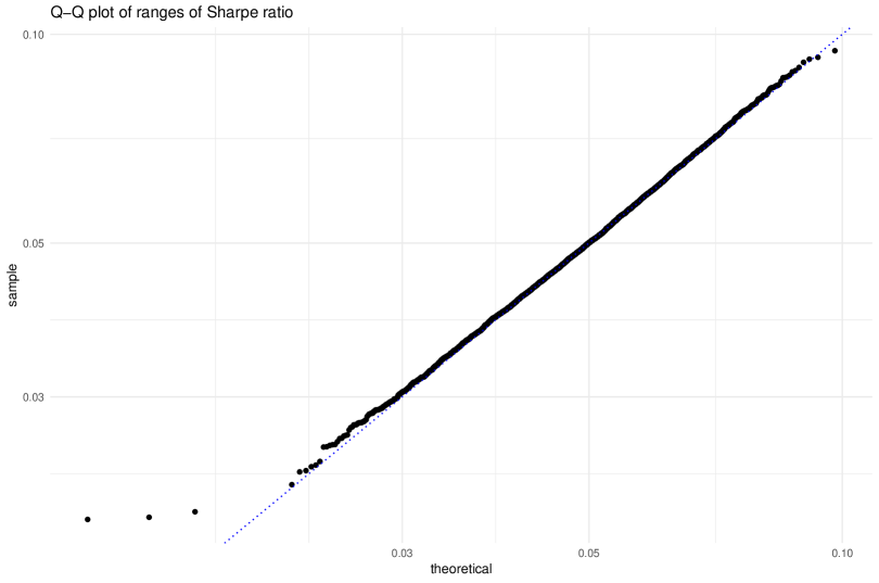
Figure 1: The quantiles of the range of Sharpe ratio from 5,000 simulations are plotted against a transformed Tukey distribution, $\sqrt{(1-\rho)/n}\,{q}_{{\cdot},{p},{\infty}}$. The points show little deviation from the plotted $y=x$ line.

We then convert these simulated ranges to p-values via the ptukey function in R, using the $df=\infty$ cutoff and the actual $\rho$. We Q-Q plot these putative p-values against a uniform law in Figure 2, and again find very good agreement. To check the tails we have transformed the p-values to $p\mapsto\left|2p-1\right|$ and plotted in log-log scale.

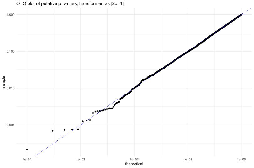
Figure 2: The computed p-values from 5,000 simulations are plotted against a uniform law, visually confirming that the p-values are nearly uniform. Simulations use the exact $\rho$ to compute the p-values via ptukey. We transform the p-values and plot $\left|2p-1\right|$ in log-log space to emphasize the tails. The points show little deviation from the plotted $y=x$ line.

Varying $n$ and $p$:

Next we perform the same kind of simulations, but vary the number of days observed in each simulation, $n$, as well as the number of different assets, $p$. We let the former vary from 20 to 1,280 measured in days, and the latter vary from 8 to 32. We take $\mathsf{R}={\rho}\left(\boldsymbol{1}{{\boldsymbol{1}}^{\top}}\right)+{\left(1-\rho\right)}\,\mathsf{I},$ for $\rho=0.8$ and set the signal-noise ratio to $1{{\mbox{yr}}^{-1/2}}$. We assume $252$ days per year for annualizing the Sharpe ratio. For each set of $50,000$ simulations, we compute the empirical type I rate at the nominal $0.05$ level by comparing the range to the HSD cutoff. We tabulate rejections using both the $df=\infty$ and $df=n-1$ cutoffs.

We plot that type I rate against $n$ in Figure 3 for the different values of $p$. For the $df=\infty$ cutoff, the procedure is apparently anticonservative, yielding too many type I errors, when the sample size is small and the number of assets is large. For the $df=n-1$ cutoff, however, the nominal type I rate is approximately achieved.

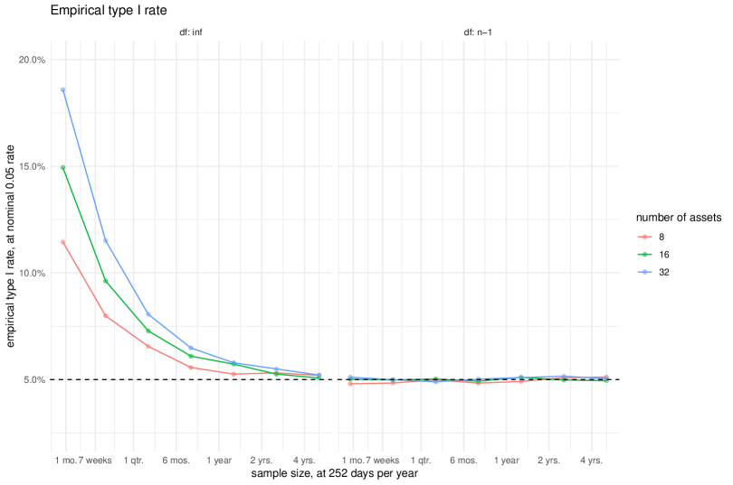
Figure 3: The empirical type I rate at the nominal 0.05 level is plotted against the number of days in each simulation, for different values of $p$. Simulations use the exact $\rho$ to perform the hypothesis test. The two facets show rejection rates under the $df=n-1$ and $df=\infty$ cutoffs. When using the $df=\infty$ cutoff, the test is anti-conservative for the “large $p$, small $n$” case, but the nominal rate is nearly achieved for the $df=n-1$ cutoff.

Varying $\rho$:

We next perform the same simulations under the null, with $\mathsf{R}={\rho}\left(\boldsymbol{1}{{\boldsymbol{1}}^{\top}}\right)+{\left(1-\rho\right)}\,\mathsf{I},$ but scanning through $\rho$. We set $n=1,008$ days, $p=16$, and set the signal-noise ratio to $1{{\mbox{yr}}^{-1/2}}$. We compute the empirical type I rate at the nominal $0.05$ level for each set of $50,000$ simulations. We plot that type I rate against $\rho$ in Figure 4. For these values of $n,p$, the procedure achieves near nominal type I rate, and does not vary in a systematic way with $\rho$.

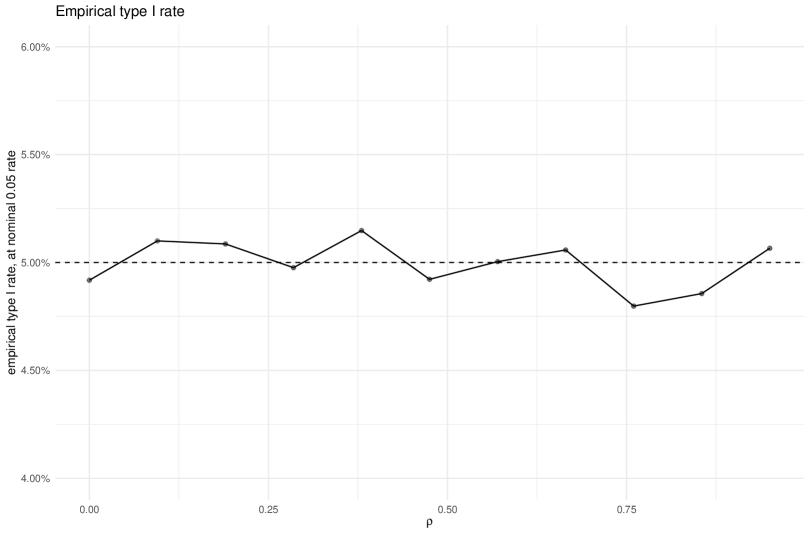
Figure 4: The empirical type I rate at the nominal 0.05 level is plotted against the correlation, $\rho$. Simulations use the exact $\rho$ to perform the hypothesis test, and the $df=n-1$ cutoff.

Feasible Estimator, Varying $\rho$:

In the simulations above we have used the actual $\rho$ in computing the threshold for rejection of the null. We repeat the experiments using a feasible test where we esimate $\rho$ from the sample. We compute the correlation of returns, then take the median value of the upper triangle of the correlation matrix.

In the first set of simulations, the true correlation matrix follows $\mathsf{R}={\rho}\left(\boldsymbol{1}{{\boldsymbol{1}}^{\top}}\right)+{\left(1-\rho\right)}\,\mathsf{I}.$ We set $n=1,008$ days, $p=16$, and set the signal-noise ratio to $1{{\mbox{yr}}^{-1/2}}$. We compute the empirical type I rate at the nominal $0.05$ level for each set of $50,000$ simulations. We plot that type I rate against $\rho$ in Figure 5. For these values of $n,p$, the procedure achieves near nominal type I rate, and does not appear to suffer from having estimated the $\rho$. In fact the plot greatly resembles Figure 4 where we have used the actual $\rho$.

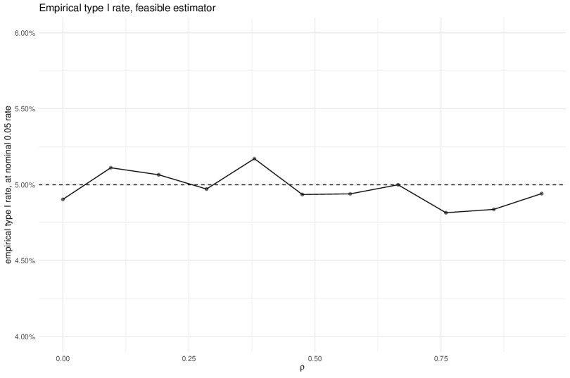
Figure 5: The empirical type I rate at the nominal 0.05 level is plotted against the correlation, $\rho$. Simulations use an estimated $\rho$ to perform the hypothesis test, and the $df=n-1$ cutoff.

Feasible Estimator, Misspecified Model, Varying $\rho$:

We repeat those simulations, estimating the $\rho$ from the sample, but now we let the correlation matrix take an “AR(1)” structure. That is, we let ${\mathsf{\hat{R}}}^{i,j}=\rho^{\left|i-j\right|}$, and vary $\rho$. Again we have $n=1,008$ days, $p=16$, the signal-noise ratio is equal to $1{{\mbox{yr}}^{-1/2}}$. We compute the empirical type I rate at the nominal $0.05$ level for each set of $50,000$ simulations.

For these simulations, we also record the type I rate when the $\rho$ is not estimated, but instead assumed to be $0$. Given that $\rho=0$ forms a kind of ‘stochastic lower bound’, we expect that the procedure will be anti-conservative when performed this way. Indeed we see in the plot that the empirical type I rate decreases to zero in increasing $\rho$. For the case where we take the median sample correlation as the estimate of $\rho$, the procedure is somewhat conservative for small $\rho$, then anti-conservative for large $\rho$. This is not surprising: for large $\rho$, the median element of $\mathsf{\hat{R}}$ will be fairly large, but the correlation among assets is somewhat weak. A more robust heuristic for estimating the $\rho$ is needed.

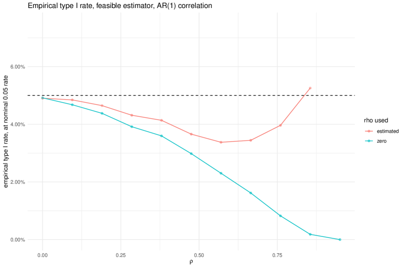
Figure 6: The empirical type I rate at the nominal 0.05 level is plotted against the correlation, $\rho$, for simulations where the correlation follows an AR(1) structure. Simulations use an estimated $\rho$ to perform the hypothesis test, and the $df=n-1$ cutoff. We include separate lines for the cases where $\rho$ is estimated, and for where it is assumed to equal $0$. For the estimated $\rho$, the procedure is conservative for small and moderate $\rho$, but anticonservative for $\rho$ near 1. When $\rho=0$ is assumed, the procedure is increasingly conservative in $\rho$.

3.2 Simulations under the alternative

We next perform the same simulations under the alternative. It is somewhat difficult to quantify the power of this procedure because the procedure can reject multiple nulls for a given experiment. Indeed, in the simulations under the null above, we analyzed the rate of any rejections for the multiple comparisons performed in a single simulation.

Under the alternative, one good:

In the first set of simulations we let $\boldsymbol{\zeta}$ have a single non-zero value, call it $\zeta$, and vary that $\zeta$. We then compute, as the ‘range’, the Sharpe ratio of the single good asset minus the minimum Sharpe ratio of the $p-1$ remaining assets. Because we are only testing $p-1$ comparisons, rather than ${p\choose 2}$, we expect to see fewer than the nominal type I rate when $\zeta=0$. Moreover, we are performing a one-sided test. As such it may be more natural to compare the rejection rate to $\alpha/2$.

We take $\mathsf{R}={\rho}\left(\boldsymbol{1}{{\boldsymbol{1}}^{\top}}\right)+{\left(1-\rho\right)}\,\mathsf{I},$ letting $\rho$ vary from 0 to 0.9; we set $n=1,008$ days, $p=16$, and let $\zeta$ vary from $0{{\mbox{yr}}^{-1/2}}$ to $1.5{{\mbox{yr}}^{-1/2}}$.

We compute the rejection rate at the nominal $0.05$ level for each set of $10,000$ simulations. We plot that (true) rejection rate against $\zeta$ in Figure 7. For these values of $n,p$, the procedure is fairly weak, only achieving power of one half for large $\zeta$ or highly correlated assets. It is not surprising that the power is increasing in $\rho$: one expects less spread among the assets for higher $\rho$, thus a true difference in signal-noise ratio is more easily detected. This same effect is visible in the paired test for equality of signal-noise ratios. [10]

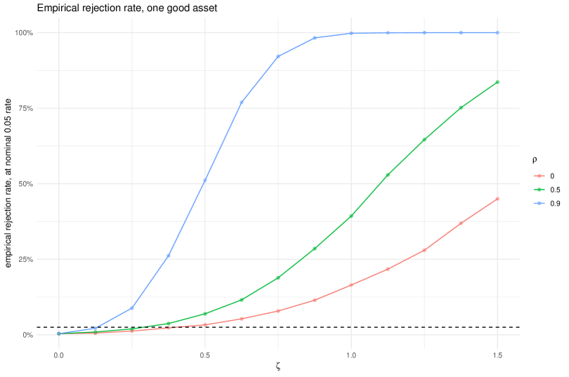
Figure 7: The empirical rejection rate at the nominal 0.05 level is plotted against the correlation, $\rho$. The population consists of one good asset with signal-noise ratio equal to $\zeta$, and the remainder with zero signal-noise ratio. Rejection is based on the Sharpe ratio of the single good asset minus the minimum Sharpe ratio of the remaining assets. Simulations use the exact $\rho$ to perform the hypothesis test, and the $df=n-1$ cutoff. We plot a horizontal line at half the nominal type I rate, 0.025, because we are performing a one-sided test.

Under the alternative, half good:

We repeat those experiments, but set half the $16$ assets to have signal-noise ratio equal to $\zeta$, and the rest to have zero signal-noise ratio. We compute, as the ‘range’, the maximum Sharpe ratio of the good assets minus the minimum Sharpe ratio of the $p-1$ remaining assets. We are effectively testing $\left(p/2\right)^{2}$ comparisons, Because we are only testing $p-1$ comparisons, rather than ${p\choose 2}$, so we expect to see fewer than the nominal type I rate when $\zeta=0$.

As above we take $\mathsf{R}={\rho}\left(\boldsymbol{1}{{\boldsymbol{1}}^{\top}}\right)+{\left(1-\rho\right)}\,\mathsf{I},$ let $\rho$ vary from 0 to 0.9, $n=1,008$ days, $p=16$, and let $\zeta$ vary from $0{{\mbox{yr}}^{-1/2}}$ to $1.5{{\mbox{yr}}^{-1/2}}$.

We compute the rejection rate at the nominal $0.05$ level for each set of $10,000$ simulations. We plot that (true) rejection rate against $\zeta$ in Figure 8. For these values of $n,p$, the procedure is again fairly underpowered, with higher power for more correlated assets.

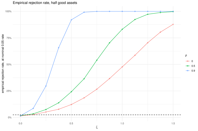
Figure 8: The empirical rejection rate at the nominal 0.05 level is plotted against the correlation, $\rho$. The population consists of half good assets with signal-noise ratio equal to $\zeta$, and the remainder with zero signal-noise ratio. Rejection is based on the maximum Sharpe ratio of the good assets minus the minimum Sharpe ratio of the remaining assets. Simulations use the exact $\rho$ to perform the hypothesis test, and the $df=n-1$ cutoff. We plot a horizontal line at half the nominal type I rate, 0.025, because we are performing a one-sided test.

3.3 Real Assets

We now apply the technique to real asset returns.

Five Industry Portfolios:

We consider the 5 industry portfolios, whose returns are computed and distributed by French. [3] The dataset consists of 1104 months of returns, from Jan 1927 to Dec 2018. The returns are highly correlated, and the correlation matrix is likely well modeled by the form ${\rho}\left(\boldsymbol{1}{{\boldsymbol{1}}^{\top}}\right)+{\left(1-\rho\right)}\,\mathsf{I},$ with $\rho$ estimated as approximately $0.8$. The Sharpe ratios range from $0.485{{\mbox{yr}}^{-1/2}}$ for Other to $0.667{{\mbox{yr}}^{-1/2}}$ for Healthcare.

First we perform the hypothesis test of equality of signal-noise ratios, as proposed by Wright et al. [17] We compute a statistic of $12.2$ which should be distributed as a $\chi^{2}\left(4\right)$ under the null. [10] This corresponds to a p-value of $0.016$, and we reject the null of equality of all signal-noise ratios.

Using the $df=n-1$ formulation and the estimated $\rho$, we compute $HSD=0.18{{\mbox{yr}}^{-1/2}}$ for $\alpha=0.05$, and narrowly reject the equality of signal-noise ratios for Other and Healthcare. In Figure 9, we plot these Sharpe ratios, along with error bars at plus and minus one $HSD$.

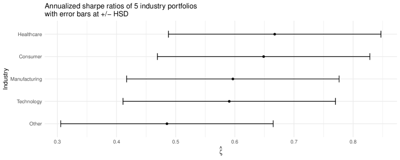
Figure 9: The annualized Sharpe ratio of French’s 5 industry portfolios are plotted, as computed on monthly returns from Jan 1927 to Dec 2018. We plot error bars at $\pm HSD$ for $\alpha=0.05$. We narrowly reject equality of the signal-noise ratio of Other and Healthcare.

Sharpe’s 34 Mutual Funds:

We consider the returns of the 34 mutual funds described by Sharpe in his original paper. [14] We transcribed the annualized percent return and standard deviation values from Sharpe’s Table I. In his paper, Sharpe computed the “reward-to-variability ratio” of each using a fixed rate of $3\%$; however, we compute the Sharpe ratio without subtracting a fixed rate. The Sharpe ratios range from $0.549{{\mbox{yr}}^{-1/2}}$ for Incorporated Investors to $1.087{{\mbox{yr}}^{-1/2}}$ for American Business Shares.

We do not have access to the series of returns, and cannot estimate the correlation structure. Somewhat optimistically we make the wild guess $\rho=0.85$. Based on this value, and setting $\alpha=0.05$, we compute $HSD=0.68{{\mbox{yr}}^{-1/2}}$, and we fail to reject the null hypothesis that all signal-noise ratios are equal. In Figure 10, we plot these Sharpe ratios, along with error bars at $\pm HSD$. Given the lack of separation of the funds, it is curious that Sharpe found correlation between the in-sample and out-of-sample Sharpe ratios of his funds. [14]

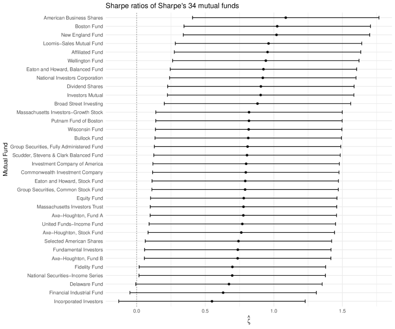
Figure 10: The annualized Sharpe ratio of Sharpe’s 34 mutual funds are plotted. Returns are from the decade 1954-1963. [14] We plot error bars at $\pm HSD$. We fail to reject the nulls that all pairwise differences are equal.

4 Future Work

A number of issues remain outstanding:

1. The heuristic use of the $df=n-1$ cutoff requires theoretical justification.

2. A stochastic inequality like Slepian’s lemma for ranges would allow one to apply the test using a lower bound $\rho$ to achieve maximum type I rate.

3. Should we expect the Tukey HSD cutoff and the Bonferroni Cutoff to be nearly equal, or will one dominate the other under certain conditions?

4. Can we quantify the power of the test?

5. Though we suspect it cannot, can the power of the test be improved?

References

- Bain and Engelhardt [1992] L. J. Bain and M. Engelhardt. Introduction to Probability and Mathematical Statistics. Classic Series. Cengage Learning, 1992. ISBN 9780534380205. URL http://books.google.com/books?id=MkFRIAAACAAJ.
- Bretz et al. [2016] Frank Bretz, Torsten Hothorn, and Peter Westfall. Multiple comparisons using R. Chapman and Hall/CRC, 2016. URL http://www.ievbras.ru/ecostat/Kiril/R/Biblio_N/R_Eng/Bretz2011.pdf.
- French [2019] Kenneth French. 5 industry portfolios. Privately Published, 2019. URL http://mba.tuck.dartmouth.edu/pages/faculty/ken.french/Data_Library/det_5_ind_port.html.
- Jobson and Korkie [1981] J. D. Jobson and Bob M. Korkie. Performance hypothesis testing with the Sharpe and Treynor measures. The Journal of Finance, 36(4):pp. 889–908, 1981. ISSN 00221082. URL http://www.jstor.org/stable/2327554.
- Johnson and Welch [1940] N. L. Johnson and B. L. Welch. Applications of the non-central t-distribution. Biometrika, 31(3-4):362–389, mar 1940. doi: 10.1093/biomet/31.3-4.362. URL http://dx.doi.org/10.1093/biomet/31.3-4.362.
- Leung and Wong [2008] Pui-Lam Leung and Wing-Keung Wong. On testing the equality of multiple Sharpe ratios, with application on the evaluation of iShares. Journal of Risk, 10(3):15–30, 2008. URL http://www.risk.net/digital_assets/4760/v10n3a2.pdf.
- Lo [2002] Andrew W. Lo. The statistics of Sharpe ratios. Financial Analysts Journal, 58(4), July/August 2002. URL http://ssrn.com/paper=377260.
- Miller and Gehr [1978] Robert E. Miller and Adam K. Gehr. Sample size bias and Sharpe’s performance measure: A note. Journal of Financial and Quantitative Analysis, 13(05):943–946, 1978. doi: 10.2307/2330636. URL https://doi.org/10.2307/2330636.
- Odeh and Evans [1974] R. E. Odeh and J. O. Evans. Algorithm AS 70: The percentage points of the normal distribution. Journal of the Royal Statistical Society. Series C (Applied Statistics), 23(1):96–97, 1974. ISSN 00359254, 14679876. doi: 10.2307/2347061. URL http://www.jstor.org/stable/2347061.
- Pav [2017] Steven E. Pav. A short Sharpe course. Privately Published, 2017. URL https://papers.ssrn.com/sol3/papers.cfm?abstract_id=3036276.
- Pav [2019] Steven E. Pav. Conditional inference on the asset with maximum Sharpe ratio. Privately Published, 2019. URL http://arxiv.org/abs/1906.00573.
- R Core Team [2015] R Core Team. R: A Language and Environment for Statistical Computing. R Foundation for Statistical Computing, Vienna, Austria, 2015. URL http://www.R-project.org/. ISBN 3-900051-07-0.
- Roy [1952] A. D. Roy. Safety first and the holding of assets. Econometrica, 20(3):pp. 431–449, 1952. ISSN 00129682. URL http://www.jstor.org/stable/1907413.
- Sharpe [1965] William F. Sharpe. Mutual fund performance. Journal of Business, 39:119, 1965. URL http://ideas.repec.org/a/ucp/jnlbus/v39y1965p119.html.
- Slepian [1962] David Slepian. The one-sided barrier problem for Gaussian noise. Bell System Technical Journal, 41(2):463–501, 1962. doi: 10.1002/j.1538-7305.1962.tb02419.x. URL https://onlinelibrary.wiley.com/doi/abs/10.1002/j.1538-7305.1962.tb02419.x.
- Tukey [1949] John W. Tukey. Comparing individual means in the analysis of variance. Biometrics, 5(2):99–114, 1949. ISSN 0006341X, 15410420. doi: 10.2307/3001913. URL http://www.jstor.org/stable/3001913.
- Wright et al. [2014] John Alexander Wright, Sheung Chi Phillip Yam, and Siu Pang Yung. A test for the equality of multiple Sharpe ratios. Journal of Risk, 16(4), 2014. URL http://www.risk.net/journal-of-risk/journal/2340044/latest-issue-of-the-journal-of-risk-volume-16-number-4-2014.
- Yin [2019] Chuancun Yin. Stochastic orderings of multivariate elliptical distributions, 2019. URL https://arxiv.org/abs/1910.07158.
- Zeitouni [2017] Ofer Zeitouni. GAUSSIAN FIELDS notes for lectures. unpublished notes, 2017. URL http://www.wisdom.weizmann.ac.il/~zeitouni/notesGauss.pdf.