Model-Free Learning of Optimal
Ergodic Policies in Wireless Systems

Abstract

Learning optimal resource allocation policies in wireless systems can be effectively achieved by formulating finite dimensional constrained programs which depend on system configuration, as well as the adopted learning parameterization. The interest here is in cases where system models are unavailable, prompting methods that probe the wireless system with candidate policies, and then use observed performance to determine better policies. This generic procedure is difficult because of the need to cull accurate gradient estimates out of these limited system queries. This paper constructs and exploits smoothed surrogates of constrained ergodic resource allocation problems, the gradients of the former being representable exactly as averages of finite differences that can be obtained through limited system probing. Leveraging this unique property, we develop a new model-free primal-dual algorithm for learning optimal ergodic resource allocations, while we rigorously analyze the relationships between original policy search problems and their surrogates, in both primal and dual domains. First, we show that both primal and dual domain surrogates are uniformly consistent approximations of their corresponding original finite dimensional counterparts. Upon further assuming the use of near-universal policy parameterizations, we also develop explicit bounds on the gap between optimal values of initial, infinite dimensional resource allocation problems, and dual values of their parameterized smoothed surrogates. In fact, we show that this duality gap decreases at a linear rate relative to smoothing and universality parameters. Thus, it can be made arbitrarily small at will, also justifying our proposed primal-dual algorithmic recipe. Numerical simulations confirm the effectiveness of our approach.

I Introduction and Problem Formulation

We investigate optimal wireless communication systems operating over realizations of random fading channels ${\mathbf{H}}\in{\mathcal{H}}\subseteq{\mathbb{R}}^{N_{{\mathbf{H}}}}$ with distribution ${\mathcal{M}}_{{\mathbf{H}}}$. Resources such as transmission power and channel access are allocated to jointly maximize the service levels of one or multiple users, in a certain sense. Due to randomness of ${\mathbf{H}}$, a reasonable objective is to optimize quality of service in an ergodic regime, i.e., by averaging all possible instantaneous service levels relative to the fading distribution ${\cal M}_{{\mathbf{H}}}$. Then, optimal wireless system design may be abstracted to a stylized base resource allocation problem of the form [1]

$$\begin{array}[]{rl}\underset{{\mathbf{x}},{\mathbf{p}}(\cdot)}{\mathrm{maximize}}&g^{o}({\mathbf{x}})\\ \mathrm{subject\,to}&{\mathbf{x}}\leq\mathbb{E}\{{\mathbf{f}}({\mathbf{p}}({\mathbf{H}}),{\mathbf{H}})\}\\ &{\mathbf{g}}({\mathbf{x}})\geq{\bf 0},\,({\mathbf{x}},{\mathbf{p}})\in{\cal X}\times{\cal P}\end{array}.$$ (1)

In (1), the policy ${\mathbf{p}}:{\mathcal{H}}\to{\mathbf{R}}^{N_{R}}$ maps fading states ${\mathbf{H}}$ to $N_{R}$ resource allocation decisions ${\mathbf{p}}({\mathbf{H}})$, the function ${\mathbf{f}}:{\mathbf{R}}^{N_{R}}\times{\mathcal{H}}\to{\mathbf{R}}^{N_{S}}$ maps decisions and fading values to $N_{S}$ instantaneous service level metrics, the average of which bounds the ergodic metrics ${\mathbf{x}}\in{\mathbf{R}}^{N_{S}}$, whose worth we evaluate through the utilities $g^{o}:{\mathbf{R}}^{N_{S}}\to{\mathbf{R}}$ and ${\mathbf{g}}:{\mathbf{R}}^{N_{S}}\to{\mathbf{R}}^{N_{{\mathbf{g}}}}$. Ergodic performances are further restricted to the set ${\mathcal{X}}\subseteq{\mathbf{R}}^{N_{S}}$ and resource allocations are further restricted to the set ${\mathcal{P}}$, the latter inducing pointwise constraints on each individual value ${\mathbf{p}}({\mathbf{H}})$ of every candidate policy ${\mathbf{p}}$ [1], for each fading realization ${\mathbf{H}}$.

Problem (1) conveniently abstracts several resource allocation tasks of practical importance. It is relatively straightforward to see that particular cases of (1) appear naturally in, e.g., point-to-point channels [1], interference channels [1, 2, 3, 4], wireless networking [1, 5, 6], as well as multiple access [7, 8], random access [9, 10] and frequency division multiplexing [11, 12, 13]. Less obvious application areas where resource allocation tasks can also be formulated as particular cases of (1) include MIMO systems [14, 15], beamforming [16, 17, 18], caching [19], and wireless control [20, 21, 22]. Although problems in [1, 5, 6, 2, 3, 4, 7, 8, 9, 10, 11, 12, 13, 14, 15, 16, 17, 18, 19, 20, 21, 22] have their own difficulties, they all share three challenges that are well-described by (1): Dimensionality, lack of convexity, and model availbaility. Indeed, when ${\mathcal{H}}$ is an infinite set –as in most applications– finding an optimal or near-optimal solution to (1) requires direct policy search, which is a rather obscure and complicated task. Further, while the utilities $g^{o}$ and ${\mathbf{g}}$ and the feasible set ${\mathcal{X}}$ are often known design choices and can be made concave or convex as needed, this is not the case with the distribution ${\mathcal{M}}_{{\mathbf{H}}}$, the service metric ${\mathbf{f}}$, or the set ${\mathcal{P}}$. These entities depend on propagation physics, as well as models of interference and multiple access management. Most often, such models are either inaccurate or unavailable, especially in complex networking settings, whereas in most existing models the form of ${\mathbf{f}}$ and ${\mathcal{P}}$ render (1) nonconvex [1].

Lack of convexity is an inherent challenge and it is accepted that we settle for locally optimal solutions, heuristics, or relaxations. To some extent, the same counts for dimensionality and model availability. However, the recent advent of machine learning for wireless communications [23, 24, 25, 26, 27, 28, 29, 30, 31, 32, 33, 34] has dawned the realization that both these challenges can be ameliorated with the incorporation of learning parametrizations [33, 34]. To see why this is true, introduce a parameterization $\boldsymbol{\phi}:{\cal H}\times\mathbb{R}^{N_{\boldsymbol{\phi}}}\rightarrow\mathbb{R}^{N_{R}}$, and restrict resource allocations as ${\mathbf{p}}(\cdot)\equiv\boldsymbol{\phi}(\cdot,\boldsymbol{\theta}),\boldsymbol{\theta}\in\mathbb{R}^{N_{\boldsymbol{\phi}}}$. Then, the base problem (1) may be relaxed as

$$\begin{array}[]{rl}\underset{{\mathbf{x}},\boldsymbol{\theta}}{\mathrm{maximize}}&g^{o}({\mathbf{x}})\\ \mathrm{subject\,to}&{\mathbf{x}}\leq\mathbb{E}\{{\mathbf{f}}(\boldsymbol{\phi}({\mathbf{H}},\boldsymbol{\theta}),{\mathbf{H}})\}\\ &{\mathbf{g}}({\mathbf{x}})\geq{\bf 0},\,({\mathbf{x}},\boldsymbol{\theta})\in{\cal X}\times\Theta\end{array},$$ (2)

where $\Theta\subseteq\big{\{}\boldsymbol{\theta}\in{\mathbf{R}}^{N_{\boldsymbol{\phi}}}\big{|}\hskip 0.50186pt\boldsymbol{\phi}(\cdot,\boldsymbol{\theta})\in{\mathcal{P}}\big{\}}$ is a nonempty and closed parameter space. Through the parametrization $\boldsymbol{\phi}$, also known as a policy function approximation (PFA) [35], problem (2) serves as a finite dimensional surrogate for the infinite dimensional problem (1) [33]. Solving such a surrogate incurs some inevitable loss of optimality. Nevertheless, this issue may be mitigated by exploiting well-known parametric function classes with universal or near-universal approximation properties such as Radial Basis Functions (RBFs) [36], Reproducing Kernel Hilbert Spaces (RKHSs) [37] and Deep Neural Networks (DNNs) [38].

While it is clear that (2) replaces infinite dimensional search by finite dimensional optimization, it is not obvious how (2) can circumvent the need for accurate models. This is addressed in [33], which builds on the observation that the PFA formulation (2) represents a scalarization of a multi-objective statistical learning problem. In fact, each entry of ${\mathbf{x}}$ is associated with an expected reward, with the difference of the two formulating a stochastic constraint. Each expected reward has the form of the objective of a greedy reinforcement learning problem [39, 40, 41, 35], in which ${\mathbf{H}}$ and $\boldsymbol{\phi}({\mathbf{H}},\boldsymbol{\theta})$ correspond to the state and control actions, respectively. In that sense, it is not only that we can reformulate optimal allocation of resources in wireless systems as a learning problem, but that learning resource allocations is inherently a learning problem. This observation led to a primal-dual training method for finding an optimal solution to (2) in [33], which relies on stochastic approximation [42, 43], and attains model-free operation borrowing randomization ideas from policy gradient methods in reinforcement learning [41].

Although the primal-dual learning algorithm of [33] has been shown to work well in some examples, including large scale networks with proper parameterizations [34], issues associated with model-free operation are not addressed. As is the case with policy gradient, the algorithm of [33] requires use of randomized policies. We know that these are inefficient as compared with deterministic policies, but we lack understanding of the loss of optimality associated with specific randomization choices. The main contribution of this paper is to put forth a principled approach for solving the PFA (2) via model-free training. We do so by avoiding the use of randomized policies altogether, and instead relying on appropriately constructed, smoothed surrogates to (2), which enable exact zeroth-order gradient representation [44]. This approach not only yields a new, efficient and technically grounded model-free training algorithm, but also enables detailed analysis, quantifying the relation of both problems (1) and (2) to the smoothed surrogate corresponding to the latter, in both primal and dual domains. Specifically, our contributions are as follows.

The Primal Smoothed Surrogate (Section III). We introduce a new smoothed surrogate to the constrained parameterized problem (2), for which we establish consistency, as well as explicit approximation rates. Our construction leverages recent results on function approximation via Gaussian convolution [44], and ensures that both the objective and constraints of the proposed smoothed surrogate approximate those of (2) uniformly in their feasible sets, under mild regularity conditions (Lemmata 3 and 4). The quality of the approximation is controlled by user-prescribed, nonnegative smoothing parameters $\mu_{S}$ and $\mu_{R}$, each associated with the decision variables ${\mathbf{x}}$ and $\boldsymbol{\theta}$ of (2), respectively. The proposed surrogate exhibits rather desirable properties. First, as either of the smoothing parameters decreases, the corresponding approximation errors shrink, and at a linear rate. Second, all smoothed approximations involved are always differentiable, and their gradients may be represented exactly as averages of finite differences, which are uniformly stable relative to both $\mu_{S}$ and $\mu_{R}$. Consequently, such approximations can be exploited to define zeroth-order stochastic quasi-gradients of the objective and all constraints of (2), with consistent and predictable behavior. Third, it is possible to establish simple and easily satisfiable conditions on (2), which ensure well-definiteness and consistency of the smoothed surrogate, as well as feasibility within the feasible sets of both (2) and (1) (Theorems 6 and 7).

The Dual Smoothed Surrogate (Section IV-A). We analyze the dual of our smoothed surrogate as a smoothed approximation to the dual of (2). We establish explicit upper and lower bounds on the difference of the respective dual optimal values, with both bounds being linearly decreasing relative to both $\mu_{S}$ and $\mu_{R}$ (Theorem 11). This result is of independent interest, because it is the first to confirm that Gaussian smoothing can be effectively leveraged in the dual domain the design of general zeroth-order (model-free) methods, applicable to constrained programs and, more broadly, problems of the saddle point type.

Duality Gap of Smoothed Surrogates (Section IV-B). Assuming an $\epsilon$-universal policy parameterization, we take [33] strictly one step further by completely characterizing the duality gap between the optimal value of the variational problem (1) and the dual value of the proposed smoothed surrogate. Specifically, we show that the aforementioned duality gap is, in absolute value, of the order of ${\cal O}(\mu_{S}{\textstyle\sqrt{N_{S}}}+\mu_{R}{\textstyle\sqrt{N_{\boldsymbol{\phi}}}}+\epsilon)$ (Theorem 15). If $\mu_{S}\equiv\mu_{R}\equiv 0$, our duality result recovers exactly that developed earlier in [33], whereas, for $\mu_{S}>0$ and $\mu_{R}>0$, it explicitly quantifies the combined effects of both policy parameterization and smoothing on approximating the optimal value of the original problem (1) via surrogate dualization.

Model-Free Learning (Section V). We develop a new randomized zeroth-order primal-dual algorithm for tackling (2), which exploits the stochastic zeroth-order gradient representation of our proposed smoothed approximations, and fits the desired model-free setting by construction. Our primal-dual algorithm is similar to that proposed in [33], but with a couple of twists; it takes advantage of our sensitivity and duality analyses and, compared to the policy gradient approach of [33], it requires no policy randomization, and it operates exclusively on probing $g^{o}$, ${\mathbf{g}}$ and the composition ${\mathbf{f}}(\boldsymbol{\phi}({\mathbf{H}},\cdot),{\mathbf{H}})$, without the need of computing the gradient of the parametric representation $\boldsymbol{\phi}({\mathbf{H}},\cdot)$. Further, the proposed algorithm converges at least to a stationary point of the dualized smoothed surrogate, which satisfies our duality gap guarantees; its optimal value can be made arbitrarily close to the optimal value of the original resource allocation problem (1) at will, by properly selecting smoothing parameters $\mu_{S}$ and $\mu_{R}$, as well as an $\epsilon$-universal parameterization $\boldsymbol{\phi}$.

Our contributions are also supported by indicative numerical simulations (Section VI), justifying our approach and confirming our theoretical findings. Indeed, our simulations demonstrate near-ideal performance of the proposed model-free method, as compared to both strictly optimal solutions and state-of-the-art heuristics, both relying on availability of explicit system models.

In the analysis that follows, we assume that the feasible set of (1) is nonempty, that ${\mathbb{E}}\{{\mathbf{f}}({\mathbf{p}}({\mathbf{H}}),{\mathbf{H}})\}$ exists and is finite for every ${\mathbf{p}}\in{\mathcal{P}}$, and that the optimal value of (1), $\mathscr{P}^{*}\in(-\infty,\infty]$, is attained for at least one feasible decision; thus, $\mathscr{P}^{*}<\infty$. Similar to (1), we assume that (2) has at least one feasible point, as well. Then, if $\mathscr{P}_{\boldsymbol{\phi}}^{*}\in(-\infty,\infty]$ denotes the optimal value of (2), it follows that $\mathscr{P}_{\boldsymbol{\phi}}^{*}\leq\mathscr{P}^{*}$, implying that $\mathscr{P}_{\boldsymbol{\phi}}^{*}<\infty$. For simplicity, we also assume that $\mathscr{P}_{\boldsymbol{\phi}}^{*}$ is attained within the feasible set of (2).

II Smoothing via Gaussian Convolution

This section introduces Gaussian smoothing and its properties, and follows closely the corresponding treatment in [44].

Let $f:{\mathbf{R}}^{N}\to{\mathbf{R}}$ be Borel. Also, for any random element $\boldsymbol{U}:\Omega\to{\mathbf{R}}^{N}$ following the standard Gaussian measure on ${\mathbf{R}}^{N}$, hereafter denoted as $\boldsymbol{U}\sim{\cal N}\left({\bf 0},\boldsymbol{I}_{N}\right)$, and for $\mu\geq 0$, consider another Borel function $f_{\mu}:{\mathbf{R}}^{N}\to{\mathbf{R}}$, defined, for every ${\mathbf{x}}\in{\mathbf{R}}^{N}$, as

$$f_{\mu}\left({\mathbf{x}}\right)\triangleq{\mathbb{E}}\left\{f\left({\mathbf{x}}+\mu\boldsymbol{U}\right)\right\}\equiv\int f\left({\mathbf{x}}+\mu\boldsymbol{u}\right){\cal N}\left(\boldsymbol{u}\right)\text{d}\boldsymbol{u},$$ (3)

with ${\cal N}:{\mathbf{R}}^{N}\to{\mathbf{R}}$ being the standard Gaussian density, i.e.,

$${\cal N}\left(\boldsymbol{u}\right)\triangleq\left(2\pi\right)^{-N/2}\exp\bigl{(}-\left\|\boldsymbol{u}\right\|_{2}^{2}/2\bigr{)},\quad\boldsymbol{u}\in{\mathbf{R}}^{N},$$ (4)

provided that the involved integral is well-defined. For every $\mu>0$, $f_{\mu}$ may be easily shown to be a convolution of the original function $f$ with the Gaussian density on ${\mathbf{R}}^{N}$ with mean zero and covariance equal to $\mu^{2}\boldsymbol{I}_{N}$. Indeed, for every ${\mathbf{x}}\in{\mathbf{R}}^{N}$, and via a simple change of variables, it is true that

$$f_{\mu}\left({\mathbf{x}}\right) =\int f\left(\boldsymbol{u}\right)\mu^{-N}{\cal N}\left(\dfrac{{\mathbf{x}}-\boldsymbol{u}}{\mu}\right)\text{d}\boldsymbol{u}$$

$$\equiv\bigl{(}f*\big{[}\mu^{-N}{\cal N}\bigl{(}\left(\cdot\right)\mu^{-1}\bigr{)}\big{]}\bigr{)}\left({\mathbf{x}}\right).$$ (5)

Therefore, the smoothed function $f_{\mu}$ may be seen as the output of a linear filter whose impulse response is the standard gaussian pulse, taking $f$ as its input.

In many cases, $f_{\mu}$ turns out to be everywhere differentiable on ${\mathbf{R}}^{N}$, even if $f$ is not, whereas the gradient of $f_{\mu}$ admits a zeroth-order representation. In particular, such is the case of all Lipschitz functions on ${\mathbf{R}}^{N}$ [44], as the next result suggests.

Lemma 1.

(Properties of $f_{\mu}$ [44]) Let $\boldsymbol{U}\sim{\cal N}\left({\bf 0},\boldsymbol{I}_{N}\right)$, and consider any globally Lipschitz function $f:{\mathbf{R}}^{N}\to{\mathbf{R}}$. Then, for any ${\cal F}\subseteq{\mathbf{R}}^{N}$, the following statements are true:

• For every $\mu\geq 0$, $f_{\mu}$ is well-defined and finite on ${\cal F}$, and

  $$\sup_{{\mathbf{x}}\in{\cal F}}|f_{\mu}\left({\mathbf{x}}\right)-f\left({\mathbf{x}}\right)|\leq\mu L\sqrt{N}.$$ (6)

• If $f$ is convex on ${\mathbf{R}}^{N}$, so is $f_{\mu}$, and $f_{\mu}\geq f$ on ${\cal F}$.

• For every $\mu>0$, $f_{\mu}$ is differentiable on ${\cal F}$, and its gradient $\nabla f_{\mu}:{\mathbf{R}}^{N}\to{\mathbf{R}}^{N}$ admits the representation

  $$\nabla f_{\mu}\left({\mathbf{x}}\right) \equiv{\mathbb{E}}\bigg{\{}\dfrac{f\left({\mathbf{x}}+\mu\boldsymbol{U}\right)-f\left({\mathbf{x}}\right)}{\mu}\boldsymbol{U}\bigg{\}},$$ (7)

  for all ${\mathbf{x}}\in{\cal F}$. Further, it is true that

  $$\sup_{{\mathbf{x}}\in{\cal F}}{\mathbb{E}}\left\{\bigg{\|}\dfrac{f\left({\mathbf{x}}+\mu\boldsymbol{U}\right)-f\left({\mathbf{x}}\right)}{\mu}\boldsymbol{U}\bigg{\|}_{2}^{2}\right\} \leq L^{2}(N+4)^{2}.$$ (8)

Lemma 1 will be key to the results presented in this paper, as discussed in detail as follows.

III Smoothed Constrained Program Surrogates

In this section, we introduce a new, smoothed surrogate of the whole constrained program (2), as promised in Section I, leveraging the results of Section II. We also introduce conditions under which this smoothed surrogate is well-defined, and establish various of its properties, as well as its structural relation to (2). The power of the proposed surrogate is in that it provides a technically grounded means for dealing with (2) in the model-free setting, i.e., when the functions $g^{o}$, ${\mathbf{g}}$ and ${\mathbf{f}}$ are apriori unknown, and may be only observed through limited probing.

III-A Surrogate Construction

Let $\mu_{S}\geq 0$, $\mu_{R}\geq 0$, and consider random elements $\boldsymbol{U}_{S}\sim{\cal N}(\boldsymbol{0},\boldsymbol{I}_{N_{S}})$ and $\boldsymbol{U}_{R}\sim{\cal N}(\boldsymbol{0},\boldsymbol{I}_{N_{\boldsymbol{\phi}}})$, the latter taken independent of ${\mathbf{H}}$. Driven by the results of Section II, we define smoothed versions of $g^{o}$, ${\mathbf{g}}$ and ${\mathbb{E}}\{{\mathbf{f}}(\boldsymbol{\phi}({\mathbf{H}},\cdot),{\mathbf{H}})\}\triangleq\overline{{\mathbf{f}}}^{\boldsymbol{\phi}}(\cdot)$ as

$$g_{\mu_{S}}^{o}({\mathbf{x}}) \triangleq{\mathbb{E}}\{g^{o}({\mathbf{x}}+\mu_{S}\boldsymbol{U}_{S})\},\quad{\mathbf{x}}\in{\mathcal{X}},$$ (9)

$${\mathbf{g}}_{\mu_{S}}({\mathbf{x}}) \triangleq{\mathbb{E}}\{{\mathbf{g}}({\mathbf{x}}+\mu_{S}\boldsymbol{U}_{S})\},\quad{\mathbf{x}}\in{\mathcal{X}}\quad\text{and}$$ (10)

$$\overline{{\mathbf{f}}}_{\mu_{R}}^{\boldsymbol{\phi}}(\boldsymbol{\theta}) \triangleq{\mathbb{E}}\{{\mathbf{f}}(\boldsymbol{\phi}({\mathbf{H}},\boldsymbol{\theta}+\mu_{R}\boldsymbol{U}_{R}),{\mathbf{H}})\},\quad\boldsymbol{\theta}\in\Theta,$$ (11)

where, at this point, we arbitrarily assume that the involved expectations are well-defined and finite on ${\mathcal{X}}$ and $\Theta$. We will return to those issues shortly. Then, we may formulate a (hopefully) smoothed version of problem (2) as

$$\begin{array}[]{rl}\underset{{\mathbf{x}},{\mathbf{p}}(\cdot)}{\mathrm{maximize}}&g_{\mu_{S}}^{o}({\mathbf{x}})\\ \mathrm{subject\,to}&{\mathbf{x}}+\mathtt{S}(\mu_{R})\leq\overline{{\mathbf{f}}}_{\mu_{R}}^{\boldsymbol{\phi}}(\boldsymbol{\theta})\\ &{\mathbf{g}}_{\mu_{S}}({\mathbf{x}})\geq{\bf 0},\,({\mathbf{x}},\boldsymbol{\theta})\in{\mathcal{X}}\times\Theta\end{array},$$ (12)

where $\mathtt{S}:{\mathbf{R}}_{+}\to{\mathbf{R}}_{+}^{N_{S}}$ is a nonnegative feasibility slack, with properties to be determined. Formulation of the smoothed surrogate (12) is well motivated due to the fact that, whenever the objective $g^{o}$ and all entries of the constraint vector functions ${\mathbf{g}}$ and ${\mathbf{f}}(\boldsymbol{\phi}({\mathbf{H}},\cdot),{\mathbf{H}})$ are sufficiently well-behaved, such that Lemma 1 appropriately applies, the smoothed functions $g_{\mu_{S}}^{o}$, ${\mathbf{g}}_{\mu_{S}}$ and $\overline{{\mathbf{f}}}_{\mu_{R}}^{\boldsymbol{\phi}}$ are differentiable, and the respective gradients may be represented as averages of suitably defined finite differences. This is particularly important in developing effective and predictable methods for solving problem (2) in the model-free setting: Finite differences are by construction based on function evaluations only. Thus, the surrogate (12) constitutes a natural zeroth-order proxy for dealing with the original parameterized problem (2).

However, before focusing on how to use (12) in order to solve (2), we have to make sure that (12) is a well-defined and feasible problem, and also reveal its fundamental connection to (2). These tasks are the subject of the rest of this section.

III-B Smoothing $g^{o},{\mathbf{g}}$ and $\overline{{\mathbf{f}}}^{\boldsymbol{\phi}}$

Our treatment will require imposing appropriate structure on the functions involved in (2), as we now discuss in detail. Hereafter, the $i$-th entries of ${\mathbf{g}}$ (resp. ${\mathbf{g}}_{\mu_{S}}$) and ${\mathbf{f}}$ (resp. $\overline{{\mathbf{f}}}_{\mu_{R}}^{\boldsymbol{\phi}}$) will be denoted as $g^{i}$ ($g_{\mu_{S}}^{i}$), $i\in\mathbb{N}_{N_{{\mathbf{g}}}}^{+}$ and $f^{i}$ ($\overline{f}_{\mu_{R}}^{\boldsymbol{\phi},i}$), $i\in\mathbb{N}_{N_{S}}^{+}$, respectively.

Assumption 1.

The following conditions are satisfied:

${\bf C1}$

For every $i\in\{o,\mathbb{N}_{N_{{\mathbf{g}}}}^{+}\}$, $g^{i}$ is $L_{g}^{i}$-Lipschitz on ${\mathbf{R}}^{N_{S}}$.

${\bf C2}$

For every $i\in\mathbb{N}_{N_{S}}^{+}$, there is $L_{f}^{i}<\infty$, such that

$$\hskip 6.0pt\|f^{i}(\boldsymbol{\phi}({\mathbf{H}},\boldsymbol{\theta}_{1}),{\mathbf{H}})-f^{i}(\boldsymbol{\phi}({\mathbf{H}},\boldsymbol{\theta}_{2}),{\mathbf{H}})\|_{{\cal L}_{2}}\\ \;\leq L_{f}^{i}\|\boldsymbol{\theta}_{1}-\boldsymbol{\theta}_{2}\|_{2},\,\forall\,(\boldsymbol{\theta}_{1},\boldsymbol{\theta}_{2})\in{\mathbf{R}}^{N_{\boldsymbol{\phi}}}\times{\mathbf{R}}^{N_{\boldsymbol{\phi}}}.\hskip 8.0pt$$ (13)

Condition $\mathbf{C2}$ of Assumption 1 has the following consequences on the behavior of ${\mathbb{E}}\{{\mathbf{f}}(\boldsymbol{\phi}({\mathbf{H}},\cdot),{\mathbf{H}})\}\equiv\overline{{\mathbf{f}}}^{\boldsymbol{\phi}}(\cdot)$.

Proposition 2.

(Properties of $\overline{{\mathbf{f}}}^{\boldsymbol{\phi}}$) Suppose that condition $\mathbf{C2}$ of Assumption 2 is in effect. Then, for every $i\in\mathbb{N}_{N_{S}}^{+}$, $\overline{f}^{\boldsymbol{\phi},i}$ is $L_{f}^{i}$-Lipschitz on ${\mathbf{R}}^{N_{\boldsymbol{\phi}}}$. Additionally, it is true that

$$\quad\quad{\mathbb{E}}\{|f^{i}(\boldsymbol{\phi}({\mathbf{H}},\boldsymbol{\theta}+\boldsymbol{u}),{\mathbf{H}})|\}\\ \leq L_{f}^{i}\|\boldsymbol{u}\|_{2}+{\mathbb{E}}\{|f^{i}(\boldsymbol{\phi}({\mathbf{H}},\boldsymbol{\theta}),{\mathbf{H}})|\},\quad\quad$$ (14)

for all $\left(\boldsymbol{\theta},\boldsymbol{u}\right)\in\Theta\times{\mathbf{R}}^{N_{\boldsymbol{\phi}}}$, and for all $i\in\mathbb{N}_{N_{S}}^{+}$.

Proof:

The first part of the result follows immediately from condition ${\bf C2}$, by the nested structure of ${\cal L}_{p}$-spaces, and Jensen. The second part follows via an application of the triangle inequality. ∎

Assumption 1 and Proposition 2 may be further exploited to establish well-definiteness and basic properties of $g_{\mu_{S}}^{o}$, ${\mathbf{g}}_{\mu_{S}}$ and $\overline{{\mathbf{f}}}_{\mu_{R}}^{\boldsymbol{\phi}}$. To this end, for ${\mathbf{x}}\in{\mathcal{X}},\mu_{S}>0$ and for every $i\in\{o,\mathbb{N}_{N_{{\mathbf{g}}}}^{+}\}$, let us define finite differences

$$\Delta_{g}^{i}({\mathbf{x}},\mu_{S},\boldsymbol{U}_{S})\triangleq\dfrac{g^{i}({\mathbf{x}}+\mu_{S}\boldsymbol{U}_{S})-g^{i}({\mathbf{x}})}{\mu_{S}}.$$ (15)

Similarly, for $\boldsymbol{\theta}\in\Theta,\mu_{R}>0$ and for every $i\in\mathbb{N}_{N_{S}}^{+}$, define

$$\Delta_{f}^{i}(\boldsymbol{\theta},\mu_{R},\boldsymbol{U}_{R},{\mathbf{H}})\\ \triangleq\dfrac{f^{i}(\boldsymbol{\phi}({\mathbf{H}},\boldsymbol{\theta}+\mu_{R}\boldsymbol{U}_{R}),{\mathbf{H}})-f^{i}(\boldsymbol{\phi}({\mathbf{H}},\boldsymbol{\theta}),{\mathbf{H}})}{\mu_{R}}.$$ (16)

The relevant results now follow.

Lemma 3.

(Existence & Properties of $g_{\mu_{S}}^{o}$ and ${\mathbf{g}}_{\mu_{S}}$) Suppose that Assumption 1 is in effect. Then, for every $i\in\{o,\mathbb{N}_{N_{{\mathbf{g}}}}^{+}\}$ and for every $\mu_{S}>0$, each $g_{\mu_{S}}^{i}$ is a well-defined, finite, concave and everywhere differentiable underestimator of $g^{i}$ on ${\mathcal{X}}$, such that

$$\sup_{{\mathbf{x}}\in{\mathcal{X}}}|g_{\mu_{S}}^{i}\left({\mathbf{x}}\right)-g^{i}\left({\mathbf{x}}\right)| \leq\mu_{S}L_{g}^{i}{\textstyle\sqrt{N_{S}}},$$ (17)

$$\sup_{{\mathbf{x}}\in{\mathcal{X}}}{\mathbb{E}}\{\|\Delta_{g}^{i}({\mathbf{x}},\mu_{S},\boldsymbol{U}_{S})\boldsymbol{U}_{S}\|_{2}^{2}\} \leq(L_{g}^{i})^{2}(N_{S}+4)^{2}$$ (18)

$$\text{and}\quad{\mathbb{E}}\{\Delta_{g}^{i}({\mathbf{x}},\mu_{S},\boldsymbol{U}_{S})\boldsymbol{U}_{S}\} \equiv\nabla g_{\mu_{S}}^{i}\left({\mathbf{x}}\right),$$ (19)

for all ${\mathbf{x}}\in{\mathcal{X}}$.

Proof:

Trivial, see Lemma 1 (Section II). ∎

Lemma 4.

(Existence & Properties of $\overline{{\mathbf{f}}}_{\mu_{R}}^{\boldsymbol{\phi}}$) Suppose that Assumption 1 is in effect. Then, for every $i\in\mathbb{N}_{N_{S}}^{+}$ and for every $\mu_{R}>0$, each $f_{\mu_{R}}^{i}$ is well-defined, finite, differentiable everywhere on $\Theta$, such that

$$\sup_{\boldsymbol{\boldsymbol{\theta}}\in\Theta}\big{|}\overline{f}_{\mu_{R}}^{\boldsymbol{\phi},i}\left(\boldsymbol{\theta}\right)-\overline{f}^{\boldsymbol{\phi},i}\left(\boldsymbol{\boldsymbol{\theta}}\right)\big{|} \leq\mu_{R}L_{f}^{i}{\textstyle\sqrt{N_{\boldsymbol{\phi}}}},$$ (20)

$$\sup_{\boldsymbol{\theta}\in\Theta}{\mathbb{E}}\{\|\Delta_{f}^{i}(\boldsymbol{\theta},\mu_{R},\boldsymbol{U}_{R},{\mathbf{H}})\boldsymbol{U}_{R}\|_{2}^{2}\} \leq(L_{f}^{i})^{2}(N_{\boldsymbol{\phi}}+4)^{2}$$ (21)

$$\text{and}\quad{\mathbb{E}}\{\Delta_{f}^{i}(\boldsymbol{\theta},\mu_{R},\boldsymbol{U}_{R},{\mathbf{H}})\boldsymbol{U}_{R}\} \equiv\nabla\overline{f}_{\mu_{R}}^{\boldsymbol{\phi},i}\left(\boldsymbol{\theta}\right),$$ (22)

for all $\boldsymbol{\theta}\in\Theta$.

Proof:

Fix $i\in\mathbb{N}_{N_{S}}^{+}$, and consider the function $\overline{f}^{\boldsymbol{\phi},i}(\cdot)\equiv{\mathbb{E}}\{f^{i}(\boldsymbol{\phi}({\mathbf{H}},\cdot),{\mathbf{H}})\}$, which, by Proposition 2, is $L_{f}^{i}$-Lipschitz on ${\mathbf{R}}^{N_{\boldsymbol{\phi}}}$. Then, Lemma 1 implies that, for every $\mu_{R}\geq 0$,

$$\sup_{\boldsymbol{\boldsymbol{\theta}}\in\Theta}\big{|}{\mathbb{E}}\big{\{}\overline{f}^{\boldsymbol{\phi},i}\left(\boldsymbol{\theta}+\mu_{R}\boldsymbol{U}_{R}\right)\big{\}}-\overline{f}^{\boldsymbol{\phi},i}\left(\boldsymbol{\boldsymbol{\theta}}\right)\big{|}\leq\mu_{R}L_{f}^{i}{\textstyle\sqrt{N_{\boldsymbol{\phi}}}}.$$ (23)

Note that we are not done yet, since ${\mathbb{E}}\big{\{}\overline{f}^{\boldsymbol{\phi},i}\left((\cdot)+\mu_{R}\boldsymbol{U}_{R}\right)\big{\}}$ involves an iterated expectation, and not an expectation relative to the joint distribution of $\boldsymbol{U}_{R}$ and ${\mathbf{H}}$. However, again by Proposition 2, it follows that, for every $\boldsymbol{\theta}\in\Theta$,

$$\int{\mathbb{E}}\{|f^{i}(\boldsymbol{\phi}({\mathbf{H}},\boldsymbol{\theta}+\mu_{R}\boldsymbol{u}),{\mathbf{H}})|\}{\mathcal{P}}_{\boldsymbol{U}_{R}}\left(\mathrm{d}\boldsymbol{u}\right)$$

$$\leq\mu_{R}L_{f}^{i}\int\|\boldsymbol{u}\|_{2}{\mathcal{P}}_{\boldsymbol{U}_{R}}\left(\mathrm{d}\boldsymbol{u}\right)+{\mathbb{E}}\{|f^{i}(\boldsymbol{\phi}({\mathbf{H}},\boldsymbol{\theta}),{\mathbf{H}})|\}$$

$$\leq\mu_{R}L_{f}^{i}\sqrt{N_{\boldsymbol{\phi}}}+{\mathbb{E}}\{|f^{i}(\boldsymbol{\phi}({\mathbf{H}},\boldsymbol{\theta}),{\mathbf{H}})|\}<\infty.$$ (24)

Then, Fubini’s Theorem (Corollary 2.6.5 and Theorem 2.6.6 in [45]) implies that $\overline{f}_{\mu_{R}}^{\boldsymbol{\phi},i}\left(\cdot\right)\equiv{\mathbb{E}}\{f^{i}(\boldsymbol{\phi}({\mathbf{H}},(\cdot)+\mu_{R}\boldsymbol{U}_{R}),{\mathbf{H}})\}$ is finite on $\Theta$, and that

$${\mathbb{E}}\big{\{}\overline{f}^{\boldsymbol{\phi},i}\left(\boldsymbol{\theta}+\mu_{R}\boldsymbol{U}_{R}\right)\big{\}}$$

$$\equiv\int{\mathbb{E}}\{f^{i}(\boldsymbol{\phi}({\mathbf{H}},\boldsymbol{\theta}+\mu_{R}\boldsymbol{u}),{\mathbf{H}})\}{\mathcal{P}}_{\boldsymbol{U}_{R}}\left(\mathrm{d}\boldsymbol{u}\right)$$

$$\equiv\int f^{i}(\boldsymbol{\phi}({\mathbf{H}},\boldsymbol{\theta}+\mu_{R}\boldsymbol{u}),{\mathbf{H}})\left[{\mathcal{P}}_{{\mathbf{H}}}\times{\mathcal{P}}_{\boldsymbol{U}_{R}}\right]\left(\mathrm{d}\left[\boldsymbol{u},{\mathbf{H}}\right]\right)$$

$$\equiv\overline{f}_{\mu_{R}}^{\boldsymbol{\phi},i}\left(\boldsymbol{\theta}\right),\quad\forall\,\boldsymbol{\theta}\in\Theta,$$ (25)

where ${\mathbf{H}}$ and $\boldsymbol{U}_{R}$ are statistically independent by assumption; now we are done. Next, differentiability of $\overline{f}_{\mu_{R}}^{\boldsymbol{\phi},i}$, as well as the form of its gradient also follow from Lemma 1 on $\overline{f}^{\boldsymbol{\phi},i}$ and, again, (25). Finally, to verify (21), we may write (due to condition ${\bf C2}$)

$${\mathbb{E}}\{\|\Delta_{f}^{i}(\boldsymbol{\theta},\mu_{R},\boldsymbol{U}_{R},{\mathbf{H}})\boldsymbol{U}_{R}\|_{2}^{2}\}$$

$$\equiv\dfrac{1}{\mu_{R}^{2}}{\mathbb{E}}\big{\{}{\mathbb{E}}\big{\{}|f^{i}(\boldsymbol{\phi}({\mathbf{H}},\boldsymbol{\theta}+\mu_{R}\boldsymbol{U}_{R}),{\mathbf{H}})$$

$$\quad\quad\quad-f^{i}(\boldsymbol{\phi}({\mathbf{H}},\boldsymbol{\theta}),{\mathbf{H}})|^{2}|\boldsymbol{U}_{R}\big{\}}\left\|\boldsymbol{U}_{R}\right\|_{2}^{2}\big{\}}$$

$$\leq\dfrac{1}{\mu_{R}^{2}}{\mathbb{E}}\big{\{}(L_{f}^{i})^{2}\|\mu_{R}\boldsymbol{U}_{R}\|_{2}^{2}\left\|\boldsymbol{U}_{R}\right\|_{2}^{2}\big{\}}$$

$$\leq(L_{f}^{i})^{2}(N_{\boldsymbol{\phi}}+4)^{2},$$ (26)

as required. The proof is complete. ∎

Remark 5.

We would like to mention that a weaker version of Lemma 3 holds if we weaken condition ${\bf C2}$ of Assumption 1, by replacing the ${\cal L}_{2}$-norm with an ${\cal L}_{1}$-norm. In this case, the $\ell_{2}$-norm-squared inside the expectation of (21) would be replaced by a mere $\ell_{2}$-norm; essentially, only boundedness of $\|\Delta_{f}^{i}(\boldsymbol{\theta},\mu_{R},\boldsymbol{U}_{R},{\mathbf{H}})\boldsymbol{U}_{R}\|_{2}$ in ${\cal L}_{1}$ would be guaranteed, instead of boundedness in ${\cal L}_{2}$. The main reason why (21) (and therefore condition ${\bf C2}$) is desirable is that it crucially affects the behavior of gradient-based algorithms for solving problems such as (12), considered later in this work. $\blacksquare$

III-C Surrogate Feasibility

We are now in place to investigate conditions ensuring feasibility of the smoothed surrogate (12). In particular, we will be interested in conditions ensuring feasibility of (12), but are on the original parameterized problem (2). This is very important from a practical point of view, since the exact form of (12) will be, in most cases, unknown. On the other hand, feasibility of (2) should be somehow guaranteed apriori, even in the model-free setting; indeed, both resource allocation problems (1) and (2) are initially proposed by the wireless engineer, who is the one responsible for formulating meaningful resource allocation tasks.

It turns out that all that is needed for (12) to be feasible is the existence of at least one strictly feasible point for (2). What is more, (12) can be made strictly feasible at will. The relevant result follows right after we define the vectors

$$\boldsymbol{c}_{S}\triangleq\big{[}L_{g}^{1}\,\ldots\,L_{g}^{N_{{\mathbf{g}}}}\big{]}^{\boldsymbol{T}}\quad\text{and}\quad\boldsymbol{c}_{R}\triangleq\big{[}L_{f}^{1}\,\ldots\,L_{f}^{N_{S}}\big{]}^{\boldsymbol{T}},$$ (27)

and under the following assumption.

Assumption 2.

The feasibility slack $\mathtt{S}_{{\mathbf{f}}}$ is increasing around the origin, and $\lim_{\mu_{R}\downarrow 0}\mathtt{S}_{{\mathbf{f}}}(\mu_{R})\equiv\mathtt{S}_{{\mathbf{f}}}(0)\equiv{\bf 0}$.

Theorem 6.

(Surrogate Strict Feasibility) Let Assumptions 1 and 2 be in effect, and suppose that $({\mathbf{x}}^{\dagger},\boldsymbol{\theta}^{\dagger})\in{\mathbf{R}}^{N_{S}}\times{\mathbf{R}}^{N_{\boldsymbol{\phi}}}$ is a strictly feasible point of the parameterized problem (2). Then there exist $\mu_{S}^{\dagger}>0$ and $\mu_{R}^{\dagger}>0$, possibly dependent on $({\mathbf{x}}^{\dagger},\boldsymbol{\theta}^{\dagger})$, such that, for every $0\leq\mu_{S}\leq\mu_{S}^{\dagger}$ and $0\leq\mu_{R}\leq\mu_{R}^{\dagger}$, the same point $({\mathbf{x}}^{\dagger},\boldsymbol{\theta}^{\dagger})$ is strictly feasible for the smoothed surrogate (12).

Proof:

Let the point $({\mathbf{x}}^{\dagger},\boldsymbol{\theta}^{\dagger})\in{\mathbf{R}}^{N_{S}}\times{\mathbf{R}}^{N_{\boldsymbol{\phi}}}$ be strictly feasible for (2), implying that $({\mathbf{x}}^{\dagger},\boldsymbol{\theta}^{\dagger})\in{\mathcal{X}}\times\Theta$, and

$${\mathbf{g}}({\mathbf{x}}^{\dagger})\geq\mathtt{s}_{{\mathbf{g}}}^{\dagger}\quad\text{and}\quad\overline{{\mathbf{f}}}^{\boldsymbol{\phi}}(\boldsymbol{\theta}^{\dagger})-{\mathbf{x}}^{\dagger}\geq\mathtt{s}_{{\mathbf{f}}}^{\dagger},$$ (28)

for some positive slacks $\mathtt{s}_{{\mathbf{g}}}^{\dagger}\in{\mathbf{R}}_{++}^{N_{{\mathbf{g}}}}$ and $\mathtt{s}_{{\mathbf{f}}}^{\dagger}\in{\mathbf{R}}_{++}^{N_{S}}$. Also, from Lemma 3, it follows that, for every $\mu_{S}\geq 0$ and $\mu_{R}\geq 0$,

$${\mathbf{g}}({\mathbf{x}}^{\dagger}) \leq{\mathbf{g}}_{\mu_{S}}({\mathbf{x}}^{\dagger})+\mu_{S}\boldsymbol{c}_{S}{\textstyle\sqrt{N_{S}}}\quad\text{and}$$ (29)

$$\overline{{\mathbf{f}}}^{\boldsymbol{\phi}}(\boldsymbol{\theta}^{\dagger}) \leq\overline{{\mathbf{f}}}_{\mu_{R}}^{\boldsymbol{\phi}}(\boldsymbol{\theta}^{\dagger})+\mu_{R}\boldsymbol{c}_{R}{\textstyle\sqrt{N_{\boldsymbol{\phi}}}},$$ (30)

Consequently, it is true that

$${\mathbf{g}}_{\mu_{S}}({\mathbf{x}}^{\dagger}) \geq\mathtt{s}_{{\mathbf{g}}}^{\dagger}-\mu_{S}\boldsymbol{c}_{S}{\textstyle\sqrt{N_{S}}}\quad\text{and}$$ (31)

$$\overline{{\mathbf{f}}}_{\mu_{R}}^{\boldsymbol{\phi}}(\boldsymbol{\theta}^{\dagger})-{\mathbf{x}}^{\dagger} \geq\mathtt{s}_{{\mathbf{f}}}^{\dagger}-\mu_{R}\boldsymbol{c}_{R}{\textstyle\sqrt{N_{\boldsymbol{\phi}}}}.$$ (32)

Therefore, we can find $\mu_{S}^{\dagger}>0$ and $\mu_{R}^{\dagger}>0$ sufficiently small but strictly positive, such that, for every $0\leq\mu_{S}\leq\mu_{S}^{\dagger}$ and $0\leq\mu_{R}\leq\mu_{R}^{\dagger}$, the strict inequalities $\mathtt{s}_{{\mathbf{g}}}^{\dagger}-\mu_{S}\boldsymbol{c}_{S}\sqrt{N_{S}}>{\bf 0}$ and $\mathtt{s}_{{\mathbf{f}}}^{\dagger}-\mu_{R}\boldsymbol{c}_{R}\sqrt{N_{\boldsymbol{\phi}}}>\mathtt{S}(\mu_{R})$ hold. This, of course, implies that $({\mathbf{x}}^{\dagger},\boldsymbol{\theta}^{\dagger})$ is a strictly feasible point for problem (12), for all aforementioned choices of $\mu_{S}$ and $\mu_{R}$. ∎

Theorem 6 is important, as it confirms the existence of a strictly feasible point for problem (12), uniformly relative to $\mu_{S}$ and $\mu_{R}$, the latter being allowed to vary in appropriate sets, whose length is controlled by the feasibility of (2) and the feasibility slack of (12). An evident byproduct of Theorem 6 is that (12) is a feasible and, therefore, meaningful optimization problem.

Another similar question we may ask is how much the constraints of (2) are violated for every feasible solution of (12). In this respect, we may formulate the following result.

Theorem 7.

(PFA Constraint Violation) Let Assumption 1 be in effect. Then, for every $\mu_{R}\geq 0$ such that

$$\mathtt{S}(\mu_{R})-\mu_{R}\boldsymbol{c}_{R}{\textstyle\sqrt{N_{\boldsymbol{\phi}}}} \geq{\bf 0},$$ (33)

and for every $\mu_{S}\geq 0$, every feasible point of (12) is also feasible for (2). Otherwise, if (33) fails to hold, then the negative values of its left-hand-side correspond to the respective levels of maximal constraint violation for (2).

Proof:

Fix qualifying $\mu_{S}$ and $\mu_{R}$, and let the point $({\mathbf{x}}^{\mu_{S}},\boldsymbol{\theta}^{\mu_{R}})\in{\mathbf{R}}^{N_{S}}\times{\mathbf{R}}^{N_{\boldsymbol{\phi}}}$ be feasible for problem (12). Then, it is in fact true that $({\mathbf{x}}^{\mu_{S}},\boldsymbol{\theta}^{\mu_{R}})\in{\mathcal{X}}\times\Theta$, whereas from Lemma 3 it follows that

$${\mathbf{g}}({\mathbf{x}}^{\mu_{S}})\geq{\mathbf{g}}_{\mu_{S}}({\mathbf{x}}^{\mu_{S}}) \geq{\bf 0}\quad\text{and}$$ (34)

$$\overline{{\mathbf{f}}}^{\boldsymbol{\phi}}(\boldsymbol{\theta}^{\mu_{R}})-{\mathbf{x}}^{\mu_{S}}+\mu_{R}\boldsymbol{c}_{R}{\textstyle\sqrt{N_{\boldsymbol{\phi}}}} \geq\overline{{\mathbf{f}}}_{\mu_{R}}^{\boldsymbol{\phi}}(\boldsymbol{\theta}^{\mu_{R}})-{\mathbf{x}}^{\mu_{S}}$$

$$\geq\mathtt{S}(\mu_{R}).$$ (35)

Rearranging the second inequality, we obtain

$$\overline{{\mathbf{f}}}^{\boldsymbol{\phi}}(\boldsymbol{\theta}^{\mu_{R}})-{\mathbf{x}}^{\mu_{S}}\geq\mathtt{S}(\mu_{R})-\mu_{R}\boldsymbol{c}_{R}{\textstyle\sqrt{N_{\boldsymbol{\phi}}}},$$ (36)

where the right-hand-sides are independent of the feasible point $({\mathbf{x}}^{\mu_{S}},\boldsymbol{\theta}^{\mu_{R}})$. The result now readily follows. ∎

It would be useful to note that if $\mathtt{S}$ is such that condition (33) is satisfied for all qualifying $\mu_{R}$, then feasibility of (2) is ensured uniformly relative to the choice of $\mu_{R}$ (and $\mu_{S}$). This means that, whenever a solution to (12) is determined, this solution will automatically satisfy the original resource constraints of the initial parameterized problem (2).

Another important observation is that Theorems 6 and 7 are not exclusive; in other words, they can hold simultaneously. Indeed, the former concerns choosing $\mu_{S}$ and $\mu_{R}$, whereas the latter concerns choosing the slack $\mathtt{S}$, which is a function $\mu_{R}$, in a way which is compatible with Assumption 2.

As an example, one can set $\mathtt{S}(\mu_{R})\equiv\mu_{R}\boldsymbol{c}_{R}{\textstyle\sqrt{N_{\boldsymbol{\phi}}}}$, where $\mathtt{S}$ readily satisfies Assumption 2. However, this might not be a feasible choice in practice, since the entries of $\boldsymbol{c}_{R}$ will probably be unknown. Still, Theorem 7 provides a basic principle for choosing $\mathtt{S}$. For instance, the choice $\mathtt{S}(\mu_{R})\equiv\boldsymbol{C}\mu_{R}{\textstyle\sqrt{N_{\boldsymbol{\phi}}}}$ would work fine, for an appropriate constant vector $\boldsymbol{C}>{\bf 0}$, which may chosen experimentally. This last point also highlights the operational importance of Theorem 7.

IV Lagrangian Duality

A promising approach for dealing with the explicit constraints of either problems (2) or (12) is by exploiting Lagrangian Duality, which has been proven essential and undoubtedly important in analyzing and efficiently solving constrained convex optimization problems; see, e.g., [46, 47, 48]. Note, however, that, since both problems (2) and (12) are typically nonconvex, most standard results in Lagrangian Duality for convex optimization do not apply automatically.

Instead, our treatment will be based on recent results reported in [33], which in turn relies on earlier results reported in [1]. In particular, the purpose of this section is to explicitly link the smoothed surrogate (12) to the parameterized problem (2), and ultimately to the base policy search problem (1), in the dual domain, effectively characterizing the respective duality gaps. Our results essentially provide a technically grounded path to dealing with the constrained problem (1) in the model-free setting, through the zeroth-order proxy (12).

To this end, consider the Lagrangian function $\mathscr{L}_{\boldsymbol{\phi}}:{\mathbf{R}}^{N_{S}}\times{\mathbf{R}}^{N_{\boldsymbol{\phi}}}\times{\mathbf{R}}^{N_{{\mathbf{g}}}}\times{\mathbf{R}}^{N_{S}}\to{\mathbf{R}}$ defined as

$$\mathscr{L}_{\boldsymbol{\phi}}({\mathbf{x}},\boldsymbol{\theta},\boldsymbol{\lambda})\triangleq g^{o}({\mathbf{x}})+\left\langle\boldsymbol{\lambda}_{S},{\mathbf{g}}({\mathbf{x}})\right\rangle+\big{\langle}\boldsymbol{\lambda}_{R},\overline{{\mathbf{f}}}^{\boldsymbol{\phi}}(\boldsymbol{\theta})-{\mathbf{x}}\big{\rangle},$$ (37)

where $\boldsymbol{\lambda}\equiv(\boldsymbol{\lambda}_{S},\boldsymbol{\lambda}_{R})\in{\mathbf{R}}^{N_{{\mathbf{g}}}}\times{\mathbf{R}}^{N_{S}}$ are multipliers associated with the respective constraint of the primal problem (2). Then the dual function $\mathscr{D}_{\boldsymbol{\phi}}:{\mathbf{R}}^{N_{{\mathbf{g}}}}\times{\mathbf{R}}^{N_{S}}\to(-\infty,\infty]$ is defined as

$$\mathscr{D}_{\boldsymbol{\phi}}(\boldsymbol{\lambda})\triangleq\sup_{({\mathbf{x}},\boldsymbol{\theta})\in{\mathcal{X}}\times\Theta}\mathscr{L}({\mathbf{x}},\boldsymbol{\theta},\boldsymbol{\lambda}).$$ (38)

Since it is true that $\mathscr{P}_{\boldsymbol{\phi}}^{*}\leq\mathscr{D}_{\boldsymbol{\phi}}$ on ${\mathbf{R}}_{+}^{N_{{\mathbf{g}}}}\times{\mathbf{R}}_{+}^{N_{S}}$, it is most reasonable to consider the dual problem

$$\begin{array}[]{rl}\mathrm{minimize}&\mathscr{D}_{\boldsymbol{\phi}}(\boldsymbol{\lambda})\\ \mathrm{subject\,to}&\boldsymbol{\lambda}\geq{\bf 0}\end{array},$$ (39)

whose optimal value

$$\mathscr{D}_{\boldsymbol{\phi}}^{*}\triangleq\inf_{\boldsymbol{\lambda}\geq{\bf 0}}\mathscr{D}_{\boldsymbol{\phi}}(\boldsymbol{\lambda})\in(-\infty,\infty]$$ (40)

serves as the tightest over-estimate of the optimal value of (2), $\mathscr{P}_{\boldsymbol{\phi}}^{*}$, when knowing only $\mathscr{D}_{\boldsymbol{\phi}}$.

In the same fashion, for $\mu_{S}>0$ and $\mu_{R}>0$, we define the Lagrangian function $\mathscr{L}_{\mu}:{\mathcal{X}}\times\Theta\times{\mathbf{R}}^{N_{{\mathbf{g}}}}\times{\mathbf{R}}^{N_{S}}\to{\mathbf{R}}$ associated with the smoothed surrogate (12) as

$$\quad\mathscr{L}_{\boldsymbol{\phi},\mu}({\mathbf{x}},\boldsymbol{\theta},\boldsymbol{\lambda})\triangleq g_{\mu_{S}}^{o}({\mathbf{x}})+\left\langle\boldsymbol{\lambda}_{S},{\mathbf{g}}_{\mu_{S}}({\mathbf{x}})\right\rangle\quad\quad\\ +\big{\langle}\boldsymbol{\lambda}_{R},\overline{{\mathbf{f}}}_{\mu_{R}}^{\boldsymbol{\phi}}(\boldsymbol{\theta})-{\mathbf{x}}-\mathtt{S}(\mu_{R})\big{\rangle},\,\,\,$$ (41)

whereas the dual function $\mathscr{D}_{\boldsymbol{\phi},\mu}:{\mathbf{R}}^{N_{{\mathbf{g}}}}\times{\mathbf{R}}^{N_{S}}\to(-\infty,\infty]$ and corresponding dual infimal value are

$$\mathscr{D}_{\boldsymbol{\phi},\mu}(\boldsymbol{\lambda}) \triangleq\sup_{({\mathbf{x}},\boldsymbol{\theta})\in{\mathcal{X}}\times\Theta}\mathscr{L}_{\boldsymbol{\phi},\mu}({\mathbf{x}},\boldsymbol{\theta},\boldsymbol{\lambda})\quad\text{and}$$ (42)

$$\mathscr{D}_{\boldsymbol{\phi},\mu}^{*} \triangleq\inf_{\boldsymbol{\lambda}\geq{\bf 0}}\mathscr{D}_{\boldsymbol{\phi},\mu}(\boldsymbol{\lambda})\in(-\infty,\infty],$$ (43)

respectively. Note that the both $\mathscr{D}_{\boldsymbol{\phi}}$ and $\mathscr{D}_{\boldsymbol{\phi},\mu}$ are convex on ${\mathbf{R}}^{N_{{\mathbf{g}}}}\times{\mathbf{R}}^{N_{S}}$, as pointwise suprema of affine functions. In our analysis, we will exploit another basic assumption, as follows.

Assumption 3.

Problem (2) is strictly feasible.

Under Assumption 3, it is true that the base problem (1) is strictly feasible as well; its feasible set contains that of (2).

IV-A Dual Optimal Values

Our first task will be to explicitly relate the optimal dual values $\mathscr{D}_{\boldsymbol{\phi}}^{*}$ and $\mathscr{D}_{\boldsymbol{\phi},\mu}^{*}$. To do so, we develop and exploit the following technical results.

Lemma 8.

(Lagrangian Approximation) Let Assumption 1 be in effect, and for every $\mu_{S}\geq 0$ , $\mu_{R}\geq 0$ and $\boldsymbol{\lambda}\geq{\bf 0}$, define the nonnegative quantities

$$\Gamma_{\mu}^{l}(\boldsymbol{\lambda}) \triangleq\mu_{S}L_{g}^{o}{\textstyle\sqrt{N_{S}}}+\mu_{S}\big{\langle}\boldsymbol{\lambda}_{S},\boldsymbol{c}_{S}\big{\rangle}{\textstyle\sqrt{N_{S}}}$$

$$\quad+\mu_{R}\big{\langle}\boldsymbol{\lambda}_{R},\boldsymbol{c}_{R}\big{\rangle}{\textstyle\sqrt{N_{\boldsymbol{\phi}}}}+\big{\langle}\mathtt{S}(\mu_{R}),\boldsymbol{\lambda}_{R}\big{\rangle},\;\text{and}$$ (44)

$$\Gamma_{\mu}^{r}(\boldsymbol{\lambda}) \triangleq\mu_{R}\big{\langle}\boldsymbol{\lambda}_{R},\boldsymbol{c}_{R}\big{\rangle}{\textstyle\sqrt{N_{\boldsymbol{\phi}}}}-\big{\langle}\mathtt{S}(\mu_{R}),\boldsymbol{\lambda}_{R}\big{\rangle}.$$ (45)

Then, for every $({\mathbf{x}},\boldsymbol{\theta})\in{\mathcal{X}}\times\Theta$, it is true that

$$-\Gamma_{\mu}^{l}(\boldsymbol{\lambda})\leq\mathscr{L}_{\boldsymbol{\phi},\mu}({\mathbf{x}},\boldsymbol{\theta},\boldsymbol{\lambda})-\mathscr{L}_{\boldsymbol{\phi}}({\mathbf{x}},\boldsymbol{\theta},\boldsymbol{\lambda})\leq\Gamma_{\mu}^{r}(\boldsymbol{\lambda}).$$ (46)

Proof:

Let $\mu_{S}\geq 0$ and $\mu_{R}\geq 0$. Since Assumption 1 is in effect, Lemma 3 implies that, for every $({\mathbf{x}},\boldsymbol{\theta},\boldsymbol{\lambda})\in{\mathcal{X}}\times\Theta\times{\mathbf{R}}_{+}^{N_{{\mathbf{g}}}}\times{\mathbf{R}}_{+}^{N_{S}}$,

$$\mathscr{L}_{\boldsymbol{\phi},\mu}({\mathbf{x}},\boldsymbol{\theta},\boldsymbol{\lambda})$$

$$\equiv g_{\mu_{S}}^{o}({\mathbf{x}})+\left\langle\boldsymbol{\lambda}_{S},{\mathbf{g}}_{\mu_{S}}({\mathbf{x}})\right\rangle+\big{\langle}\boldsymbol{\lambda}_{R},\overline{{\mathbf{f}}}_{\mu_{R}}^{\boldsymbol{\phi}}(\boldsymbol{\theta})-{\mathbf{x}}-\mathtt{S}(\mu_{R})\big{\rangle}$$

$$\leq g^{o}({\mathbf{x}})+\left\langle\boldsymbol{\lambda}_{S},{\mathbf{g}}({\mathbf{x}})\right\rangle+\big{\langle}\boldsymbol{\lambda}_{R},\overline{{\mathbf{f}}}^{\boldsymbol{\phi}}(\boldsymbol{\theta})-{\mathbf{x}}\big{\rangle}$$

$$\quad+\big{\langle}\boldsymbol{\lambda}_{R},\mu_{R}\boldsymbol{c}_{R}{\textstyle\sqrt{N_{\boldsymbol{\phi}}}}-\mathtt{S}(\mu_{R})\big{\rangle}$$

$$\equiv\mathscr{L}_{\boldsymbol{\phi}}({\mathbf{x}},\boldsymbol{\theta},\boldsymbol{\lambda})+\Gamma_{\mu}^{r}(\boldsymbol{\lambda}).$$ (47)

By symmetry, a similar argument is possible for $\mathscr{L}_{\boldsymbol{\phi}}$, namely,

$$\mathscr{L}_{\boldsymbol{\phi}}({\mathbf{x}},\boldsymbol{\theta},\boldsymbol{\lambda})$$

$$\equiv g^{o}({\mathbf{x}})+\left\langle\boldsymbol{\lambda}_{S},{\mathbf{g}}({\mathbf{x}})\right\rangle+\big{\langle}\boldsymbol{\lambda}_{R},\overline{{\mathbf{f}}}^{\boldsymbol{\phi}}(\boldsymbol{\theta})-{\mathbf{x}}\big{\rangle}$$

$$\leq g_{\mu_{S}}^{o}({\mathbf{x}})+\left\langle\boldsymbol{\lambda}_{S},{\mathbf{g}}_{\mu_{S}}({\mathbf{x}})\right\rangle+\big{\langle}\boldsymbol{\lambda}_{R},\overline{{\mathbf{f}}}_{\mu_{R}}^{\boldsymbol{\phi}}(\boldsymbol{\theta})-{\mathbf{x}}-\mathtt{S}(\mu_{R})\big{\rangle}$$

$$\quad+\mu_{S}L_{g}^{o}{\textstyle\sqrt{N_{S}}}+\big{\langle}\boldsymbol{\lambda}_{S},\mu_{S}\boldsymbol{c}_{S}{\textstyle\sqrt{N_{S}}}\big{\rangle}$$

$$\quad\quad+\big{\langle}\boldsymbol{\lambda}_{R},\mu_{R}\boldsymbol{c}_{R}{\textstyle\sqrt{N_{\boldsymbol{\phi}}}}\big{\rangle}+\big{\langle}\boldsymbol{\lambda}_{R},\mathtt{S}(\mu_{R})\big{\rangle}$$

$$\equiv\mathscr{L}_{\boldsymbol{\phi},\mu}({\mathbf{x}},\boldsymbol{\theta},\boldsymbol{\lambda})+\Gamma_{\mu}^{l}(\boldsymbol{\lambda}).$$ (48)

Rearranging (47) and (48) gives the result. ∎

Lemma 9.

(Dual Functions are Proper & Closed) As long as $\mathscr{D}_{\boldsymbol{\phi}}^{*}<\infty$, the dual function $\mathscr{D}_{\boldsymbol{\phi}}$ is proper and closed. If, additionally, Assumption 1 is in effect, then, for every $\mu_{S}>0$ and $\mu_{R}>0$, the smoothed dual function $\mathscr{D}_{\boldsymbol{\phi},\mu}$ is also proper and closed.

Proof:

Since $\mathscr{D}_{\boldsymbol{\phi}}^{*}<\infty$, there exists a dual feasible point $\boldsymbol{\lambda}^{\ddagger}\geq{\bf 0}$ such that $\mathscr{D}_{\boldsymbol{\phi}}(\boldsymbol{\lambda}^{\ddagger})<\infty$, whereas the fact that $\mathscr{L}_{\boldsymbol{\phi}}$ is real-valued on its domain implies that $\mathscr{D}_{\boldsymbol{\phi}}>-\infty$ on ${\mathbf{R}}^{N_{{\mathbf{g}}}}\times{\mathbf{R}}^{N_{S}}$. Then $\mathscr{D}_{\boldsymbol{\phi}}$ is proper, by definition (p. 7 in [48]).

To show that $\mathscr{D}_{\boldsymbol{\phi}}$ is also closed, it suffices to observe that it is the pointwise supremum of affine functions, each of which is continuous (thus lower semicontinuous) on the closed set ${\mathbf{R}}^{N_{{\mathbf{g}}}}\times{\mathbf{R}}^{N_{S}}$, and, therefore, closed (Proposition 1.1.3 in [48]). Then $\mathscr{D}_{\boldsymbol{\phi}}$ must be closed, by ([48], Proposition 1.1.6).

If now Assumption 1 is in effect, then for the same dual feasible point $\boldsymbol{\lambda}^{\ddagger}$ as above, and for every $({\mathbf{x}},\boldsymbol{\theta})\in{\mathcal{X}}\times\Theta$, Lemma 8 implies that

$$\mathscr{L}_{\boldsymbol{\phi},\mu}({\mathbf{x}},\boldsymbol{\theta},\boldsymbol{\lambda}^{\ddagger})\leq\mathscr{L}_{\boldsymbol{\phi}}({\mathbf{x}},\boldsymbol{\theta},\boldsymbol{\lambda}^{\ddagger})+\Gamma_{\mu}^{r}(\boldsymbol{\lambda}^{\ddagger}).$$ (49)

Therefore, it follows that

$$\mathscr{D}_{\boldsymbol{\phi},\mu}(\boldsymbol{\lambda}^{\ddagger}) \equiv\sup_{({\mathbf{x}},\boldsymbol{\theta})\in{\mathcal{X}}\times\Theta}\mathscr{L}_{\boldsymbol{\phi},\mu}({\mathbf{x}},\boldsymbol{\theta},\boldsymbol{\lambda}^{\ddagger})$$

$$\leq\bigg{[}\sup_{({\mathbf{x}},\boldsymbol{\theta})\in{\mathcal{X}}\times\Theta}\mathscr{L}_{\boldsymbol{\phi}}({\mathbf{x}},\boldsymbol{\theta},\boldsymbol{\lambda}^{\ddagger})\bigg{]}+\Gamma_{\mu}^{r}(\boldsymbol{\lambda}^{\ddagger})$$

$$\equiv\mathscr{D}_{\boldsymbol{\phi}}(\boldsymbol{\lambda}^{\ddagger})+\Gamma_{\mu}^{r}(\boldsymbol{\lambda}^{\ddagger})<\infty.$$ (50)

As before, $\mathscr{L}_{\boldsymbol{\phi},\mu}$ is real-valued on its domain, thus $\mathscr{D}_{\boldsymbol{\phi},\mu}>-\infty$ everywhere on ${\mathbf{R}}^{N_{{\mathbf{g}}}}\times{\mathbf{R}}^{N_{S}}$, showing that $\mathscr{D}_{\boldsymbol{\phi},\mu}$ is proper. Lastly, closeness of $\mathscr{D}_{\boldsymbol{\phi},\mu}$ follows by the same argument as that for $\mathscr{D}_{\boldsymbol{\phi}}$, above. ∎

Lemma 10.

(Existence of Dual Optimal Solutions) Suppose that $\mathscr{D}_{\boldsymbol{\phi}}^{*}<\infty$, and let Assumption 3 be in effect. Then, the set of dual optimal solutions $\arg\min_{\boldsymbol{\lambda}\geq{\bf 0}}\mathscr{D}_{\boldsymbol{\phi}}(\boldsymbol{\lambda})$ is nonempty and compact in ${\mathbf{R}}_{+}^{N_{{\mathbf{g}}}}\times{\mathbf{R}}_{+}^{N_{S}}$. If, additionally, Assumptions 1 and 2 are in effect, then there exist $\mu_{S}^{\dagger}>0$ and $\mu_{R}^{\dagger}>0$, such that, for every $0<\mu_{S}\leq\mu_{S}^{\dagger}$ and $0<\mu_{R}\leq\mu_{R}^{\dagger}$, the solution set $\arg\min_{\boldsymbol{\lambda}\geq{\bf 0}}\mathscr{D}_{\boldsymbol{\phi},\mu}(\boldsymbol{\lambda})$ is a nonempty and compact subset of ${\mathbf{R}}_{+}^{N_{{\mathbf{g}}}}\times{\mathbf{R}}_{+}^{N_{S}}$, as well.

Proof:

For any point $({\mathbf{x}}^{\dagger},\boldsymbol{\theta}^{\dagger})\in{\mathbf{R}}^{N_{S}}\times{\mathbf{R}}^{N_{\boldsymbol{\phi}}}$, which is strictly feasible for (2), it is true that ${\mathbf{g}}({\mathbf{x}}^{\dagger})>{\bf 0}$ and $\overline{{\mathbf{f}}}^{\boldsymbol{\phi}}(\boldsymbol{\theta}^{\dagger})-{\mathbf{x}}^{\dagger}>{\bf 0}$. Then, for every $\boldsymbol{\lambda}\geq{\bf 0}$, we have

$$\mathscr{L}_{\boldsymbol{\phi}}({\mathbf{x}}^{\dagger},\boldsymbol{\theta}^{\dagger},\boldsymbol{\lambda})\leq\mathscr{D}_{\boldsymbol{\phi}}(\boldsymbol{\lambda}),$$ (51)

where the left-hand-side is non-trivially affine in $\boldsymbol{\lambda}$. Now, consider any sequence $\{\boldsymbol{\lambda}^{n}\}_{n\in\mathbb{N}}\subseteq{\mathbf{R}}_{+}^{N_{{\mathbf{g}}}}\times{\mathbf{R}}_{+}^{N_{S}}$, such that $\lim_{n\to\infty}\|\boldsymbol{\lambda}^{n}\|_{2}\equiv\infty$. Since $\mathscr{L}_{\boldsymbol{\phi}}({\mathbf{x}}^{\dagger},\boldsymbol{\theta}^{\dagger},\cdot)$ is a non-trivial affine function and with positive slope, we may write

$$\liminf_{n\to\infty}\mathscr{D}_{\boldsymbol{\phi}}(\boldsymbol{\lambda}^{n}) \geq\liminf_{n\to\infty}\mathscr{L}_{\boldsymbol{\phi}}({\mathbf{x}}^{\dagger},\boldsymbol{\theta}^{\dagger},\boldsymbol{\lambda}^{n})$$

$$\equiv\lim_{n\to\infty}\mathscr{L}_{\boldsymbol{\phi}}({\mathbf{x}}^{\dagger},\boldsymbol{\theta}^{\dagger},\boldsymbol{\lambda}^{n})\equiv\infty,$$ (52)

which in turn yields

$$\liminf_{n\to\infty}\mathscr{D}_{\boldsymbol{\phi}}(\boldsymbol{\lambda}^{n})\equiv\infty\implies\lim_{n\to\infty}\mathscr{D}_{\boldsymbol{\phi}}(\boldsymbol{\lambda}^{n})\equiv\infty.$$ (53)

Noting that $\mathscr{D}_{\boldsymbol{\phi}}$ is proper due to $\mathscr{D}_{\boldsymbol{\phi}}^{*}$ being finite by assumption and Lemma 9, it is straightforward to show that the clipped dual function $\widetilde{\mathscr{D}}_{\boldsymbol{\phi}}:{\mathbf{R}}^{N_{{\mathbf{g}}}}\times{\mathbf{R}}^{N_{S}}\to(-\infty,\infty]$ defined as

$$\widetilde{\mathscr{D}}_{\boldsymbol{\phi}}(\boldsymbol{\lambda})\triangleq\begin{cases}\mathscr{D}_{\boldsymbol{\phi}}(\boldsymbol{\lambda}),&\text{if }\boldsymbol{\lambda}\geq{\bf 0}\\ \infty,&\text{otherwise}\end{cases}$$ (54)

is proper and coercive (p. 119 in [48]). Since, also by Lemma 9, $\mathscr{D}_{\boldsymbol{\phi}}$ is closed, it follows that $\widetilde{\mathscr{D}}_{\boldsymbol{\phi}}$ is closed as well (as a sum of proper closed functions: $\mathscr{D}_{\boldsymbol{\phi}}$ itself and the indicator of ${\mathbf{R}}_{+}^{N_{{\mathbf{g}}}}\times{\mathbf{R}}_{+}^{N_{S}}$; see ([48], Proposition 1.1.5)). Thus, we may call ([48], Proposition 3.2.1), which ensures that $\arg\min_{\boldsymbol{\lambda}\geq{\bf 0}}\mathscr{D}_{\boldsymbol{\phi}}(\boldsymbol{\lambda})$ is a nonempty and compact set in ${\mathbf{R}}_{+}^{N_{{\mathbf{g}}}}\times{\mathbf{R}}_{+}^{N_{S}}$.

Next, whenever Assumptions 1 and 2 are in effect, Theorem 6 ensures the existence of strictly positive numbers $\mu_{S}^{\dagger}>0$ and $\mu_{R}^{\dagger}>0$, possibly dependent on $({\mathbf{x}}^{\dagger},\boldsymbol{\theta}^{\dagger})$, such that, for every $0<\mu_{S}\leq\mu_{S}^{\dagger}$ and $0<\mu_{R}\leq\mu_{R}^{\dagger}$, the particular point $({\mathbf{x}}^{\dagger},\boldsymbol{\theta}^{\dagger})$ is also strictly feasible for problem (12). Then, with the help of the respective part of Lemma 9, the procedure presented above for (2) may be repeated for (12), for each pair of qualifying $\mu_{S}$ and $\mu_{R}$. ∎

Out of Lemmata 8, 9 and 10, the first and the last are the most important. In particular, Lemma 8 provides explicit non-symmetric upper and lower bounds for the difference between the Lagrangians of (2) and (12), which are independent of ${\mathbf{x}}$ and $\boldsymbol{\theta}$. Therefore, it should be possible to obtain approximation bounds on the respective dual functions, uniform relative to $({\mathbf{x}},\boldsymbol{\theta})$. On top of this, Lemma 10 verifies the existence of dual optimal solutions for (2) and (12), which could be exploited in conjunction with the aforementioned uniform bounds on the respective dual functions, to provide fundamental upper and lower bounds on the corresponding dual optimal (infimal) values. All this is confirmed and rigorously quantified by the next central result.

Theorem 11.

(Dual Value Approximation) Let Assumptions 1, 2 and 3 be in effect, and suppose that $\mathscr{D}_{\boldsymbol{\phi}}^{*}<\infty$. Then there exist $\mu_{S}^{\dagger}>0$ and $\mu_{R}^{\dagger}>0$, such that, for every $0\leq\mu_{S}\leq\mu_{S}^{\dagger}$ and $0\leq\mu_{R}\leq\mu_{R}^{\dagger}$,

$$\boxed{-\Gamma_{\mu}^{l}(\boldsymbol{\lambda}_{\boldsymbol{\phi}}^{\dagger})\leq-\Gamma_{\mu}^{l}(\boldsymbol{\lambda}_{\boldsymbol{\phi},\mu}^{*})\leq\mathscr{D}_{\boldsymbol{\phi},\mu}^{*}-\mathscr{D}_{\boldsymbol{\phi}}^{*}\leq\Gamma_{\mu}^{r}(\boldsymbol{\lambda}_{\boldsymbol{\phi}}^{*}).}$$ (55)

where $\boldsymbol{\lambda}_{\boldsymbol{\phi},\mu}^{*}\in\arg\min_{\boldsymbol{\lambda}\geq{\bf 0}}\mathscr{D}_{\boldsymbol{\phi},\mu}(\boldsymbol{\lambda})$, $\mathscr{D}_{\boldsymbol{\phi},0}^{*}\equiv\mathscr{D}_{\boldsymbol{\phi}}^{*}$ and $\boldsymbol{\lambda}_{\boldsymbol{\phi},0}^{*}\equiv\boldsymbol{\lambda}_{\boldsymbol{\phi}}^{*}$, identically, and where $\boldsymbol{\lambda}_{\boldsymbol{\phi}}^{\dagger}\geq{\bf 0}$ is a finite constant, problem dependent but independent of $\mu_{S}$ and $\mu_{R}$. Further, if $\mathtt{S}(\mu_{R})\equiv\boldsymbol{C}\mu_{R}{\textstyle\sqrt{N_{\boldsymbol{\phi}}}},\boldsymbol{C}\geq{\bf 0}$, then there always exist finite constants $\Sigma_{S}^{l}\geq 0$, $\Sigma_{R}^{l}\geq 0$ and $\Sigma_{R}^{r}\in{\mathbf{R}}$, problem dependent but independent of $\mu_{S}$ and $\mu_{R}$, such that

$$\boxed{-(\mu_{S}\Sigma_{S}^{l}+\mu_{R}\Sigma_{R}^{l})\leq\mathscr{D}_{\boldsymbol{\phi},\mu}^{*}-\mathscr{D}_{\boldsymbol{\phi}}^{*}\leq\mu_{R}\Sigma_{R}^{r}.}$$ (56)

In particular, $\Sigma_{S}^{l}$, $\Sigma_{R}^{l}$ and $\Sigma^{r}$ are defined as

$$\Sigma_{S}^{l} \triangleq\big{(}L_{g}^{o}+\big{\langle}\boldsymbol{\lambda}_{\boldsymbol{\phi},S}^{\dagger},\boldsymbol{c}_{S}\big{\rangle}\big{)}{\textstyle\sqrt{N_{S}}},$$ (57)

$$\Sigma_{R}^{l} \triangleq\big{\langle}\boldsymbol{\lambda}_{\boldsymbol{\phi},R}^{\dagger},\boldsymbol{c}_{R}+\boldsymbol{C}\big{\rangle}{\textstyle\sqrt{N_{\boldsymbol{\phi}}}}\quad\text{and}$$ (58)

$$\Sigma_{R}^{r} \triangleq\big{\langle}\boldsymbol{\lambda}_{\boldsymbol{\phi},R}^{*},\boldsymbol{c}_{R}-\boldsymbol{C}\big{\rangle}{\textstyle\sqrt{N_{\boldsymbol{\phi}}}}.$$ (59)

Lastly, whenever $\mathtt{S}(\mu_{R})\equiv\boldsymbol{C}\mu_{R}{\textstyle\sqrt{N_{\boldsymbol{\phi}}}}$ with $\boldsymbol{C}\geq\boldsymbol{c}_{R}$, then the right-hand-sides of (55) and (56) are nonpositive, and may be replaced by zero.

Proof:

Under the assumptions of the theorem, Lemma 10 ensures that the dual optimal solution set $\arg\min_{\boldsymbol{\lambda}\geq{\bf 0}}\mathscr{D}_{\boldsymbol{\phi},\mu}(\boldsymbol{\lambda})$ is nonempty, for all $0\leq\mu_{S}\leq\mu_{S}^{\dagger}$ and $0\leq\mu_{R}\leq\mu_{R}^{\dagger}$. Consequently, there exist optimal multipliers $\boldsymbol{\lambda}_{\boldsymbol{\phi},\mu}^{*}\geq{\bf 0}$, such that

$$-\infty<\mathscr{D}_{\boldsymbol{\phi},\mu}(\boldsymbol{\lambda}_{\boldsymbol{\phi},\mu}^{*})\equiv\mathscr{D}_{\boldsymbol{\phi},\mu}^{*}\equiv\inf_{\boldsymbol{\lambda\geq{\bf 0}}}\mathscr{D}_{\boldsymbol{\phi},\mu}(\boldsymbol{\lambda}),$$ (60)

for all allowable values of $\mu_{S}$ and $\mu_{R}$. Therefore, invoking Lemma 8, we may carefully write

$$\mathscr{D}_{\boldsymbol{\phi},\mu}^{*} \leq\mathscr{D}_{\boldsymbol{\phi},\mu}(\boldsymbol{\lambda}_{\boldsymbol{\phi}}^{*})$$

$$\equiv\sup_{({\mathbf{x}},\boldsymbol{\theta})\in{\mathcal{X}}\times\Theta}\mathscr{L}_{\boldsymbol{\phi},\mu}({\mathbf{x}},\boldsymbol{\theta},\boldsymbol{\lambda}_{\boldsymbol{\phi}}^{*})$$

$$\leq\bigg{[}\sup_{({\mathbf{x}},\boldsymbol{\theta})\in{\mathcal{X}}\times\Theta}\mathscr{L}_{\boldsymbol{\phi}}({\mathbf{x}},\boldsymbol{\theta},\boldsymbol{\lambda}_{\boldsymbol{\phi}}^{*})\bigg{]}+\Gamma_{\mu}^{r}(\boldsymbol{\lambda}_{\boldsymbol{\phi}}^{*})$$

$$\equiv\mathscr{D}_{\boldsymbol{\phi}}(\boldsymbol{\lambda}_{\boldsymbol{\phi}}^{*})+\Gamma_{\mu}^{r}(\boldsymbol{\lambda}_{\boldsymbol{\phi}}^{*})$$

$$\equiv\mathscr{D}_{\boldsymbol{\phi}}^{*}+\Gamma_{\mu}^{r}(\boldsymbol{\lambda}_{\boldsymbol{\phi}}^{*}).$$ (61)

By symmetry, we also have

$$\mathscr{D}_{\boldsymbol{\phi}}^{*} \leq\mathscr{D}_{\boldsymbol{\phi}}(\boldsymbol{\lambda}_{\boldsymbol{\phi},\mu}^{*})$$

$$\equiv\sup_{({\mathbf{x}},\boldsymbol{\theta})\in{\mathcal{X}}\times\Theta}\mathscr{L}_{\boldsymbol{\phi}}({\mathbf{x}},\boldsymbol{\theta},\boldsymbol{\lambda}_{\boldsymbol{\phi},\mu}^{*})$$

$$\leq\bigg{[}\sup_{({\mathbf{x}},\boldsymbol{\theta})\in{\mathcal{X}}\times\Theta}\mathscr{L}_{\boldsymbol{\phi},\mu}({\mathbf{x}},\boldsymbol{\theta},\boldsymbol{\lambda}_{\boldsymbol{\phi},\mu}^{*})\bigg{]}+\Gamma_{\mu}^{l}(\boldsymbol{\lambda}_{\boldsymbol{\phi},\mu}^{*})$$

$$\equiv\mathscr{D}_{\boldsymbol{\phi},\mu}(\boldsymbol{\lambda}_{\boldsymbol{\phi},\mu}^{*})+\Gamma_{\mu}^{l}(\boldsymbol{\lambda}_{\boldsymbol{\phi},\mu}^{*})$$

$$\equiv\mathscr{D}_{\boldsymbol{\phi}}^{*}+\Gamma_{\mu}^{l}(\boldsymbol{\lambda}_{\boldsymbol{\phi},\mu}^{*}).$$ (62)

Rearranging (61) and (62), we obtain the last three inequalities of (55) (left-to-right), as in the statement of the theorem.

Now, recalling that $\boldsymbol{\lambda}_{\boldsymbol{\phi},\mu}^{*}\equiv(\boldsymbol{\lambda}_{\boldsymbol{\phi},S}^{*}(\mu_{S}),\boldsymbol{\lambda}_{\boldsymbol{\phi},R}^{*}(\mu_{R}))$, we may define maximal multipliers (here the supremum is taken elementwise on the involved vectors)

$$\boldsymbol{\lambda}_{\boldsymbol{\phi},S}^{\dagger} \triangleq\sup_{\mu\in[0,\mu_{S}^{\dagger}]}\boldsymbol{\lambda}_{\boldsymbol{\phi},S}^{*}(\mu_{S}),\quad\text{and}$$ (63)

$$\boldsymbol{\lambda}_{\boldsymbol{\phi},R}^{\dagger} \triangleq\sup_{\mu\in[0,\mu_{R}^{\dagger}]}\boldsymbol{\lambda}_{\boldsymbol{\phi},R}^{*}(\mu_{R}).$$ (64)

Note that $\boldsymbol{\lambda}_{\boldsymbol{\phi}}^{\dagger}\equiv(\boldsymbol{\lambda}_{\boldsymbol{\phi},S}^{\dagger},\boldsymbol{\lambda}_{\boldsymbol{\phi},R}^{\dagger})\geq{\bf 0}$ is finite, since $\boldsymbol{\lambda}_{\boldsymbol{\phi},S}^{*}(\mu_{S})\geq{\bf 0}$ and $\boldsymbol{\lambda}_{\boldsymbol{\phi},R}^{*}(\mu_{R})\geq{\bf 0}$ are finite everywhere on the compact sets $[0,\mu_{S}^{\dagger}]$ and $[0,\mu_{R}^{\dagger}]$, respectively. Using these definitions, it follows that, for every $0\leq\mu_{S}\leq\mu_{S}^{\dagger}$ and $0\leq\mu_{R}\leq\mu_{R}^{\dagger}$,

$$\Gamma_{\mu}^{l}(\boldsymbol{\lambda}_{\boldsymbol{\phi},\mu}^{*})\leq\Gamma_{\mu}^{l}(\boldsymbol{\lambda}_{\boldsymbol{\phi}}^{\dagger}),$$ (65)

verifying the left inequality of (55).

When $\mathtt{S}(\mu_{R})\equiv\boldsymbol{C}\mu_{R}{\textstyle\sqrt{N_{\boldsymbol{\phi}}}},\boldsymbol{C}\geq{\bf 0}$, the rest of the claims stated in the theorem follow by noting that, for every $\boldsymbol{\lambda}\geq{\bf 0}$,

$$\Gamma_{\mu}^{l}(\boldsymbol{\lambda}) \triangleq\mu_{S}\big{(}L_{g}^{o}+\big{\langle}\boldsymbol{\lambda}_{S},\boldsymbol{c}_{S}\big{\rangle}\big{)}{\textstyle\sqrt{N_{S}}}$$

$$\quad+\mu_{R}\big{(}\big{\langle}\boldsymbol{\lambda}_{R},\boldsymbol{c}_{R}\big{\rangle}+\big{\langle}\boldsymbol{C},\boldsymbol{\lambda}_{R}\big{\rangle}\big{)}{\textstyle\sqrt{N_{\boldsymbol{\phi}}}}\quad\text{and}$$ (66)

$$\Gamma_{\mu}^{r}(\boldsymbol{\lambda}) \triangleq\mu_{R}\big{(}\big{\langle}\boldsymbol{\lambda}_{R},\boldsymbol{c}_{R}\big{\rangle}-\big{\langle}\boldsymbol{C},\boldsymbol{\lambda}_{R}\big{\rangle}\big{)}{\textstyle\sqrt{N_{\boldsymbol{\phi}}}},$$

where both functions $\Gamma_{(\cdot)}^{l}$ and $\Gamma_{(\cdot)}^{r}$ are nondecreasing in both $\mu_{S}$ and $\mu_{R}$. If, additionally, $\boldsymbol{C}\geq\boldsymbol{c}_{R}$, then $\Gamma_{(\cdot)}^{r}\leq 0$. The proof is complete. ∎

IV-B Approximate Strong Duality

After explicitly relating the dual optimal values $\mathscr{D}_{\boldsymbol{\phi}}^{*}$ and $\mathscr{D}_{\boldsymbol{\phi},\mu}^{*}$, our second task will be to relate $\mathscr{D}_{\boldsymbol{\phi},\mu}^{*}$ to the optimal value of the base problem (1). In particular, we would like to characterize the duality gap between the primal problem (1) and the dual to problem (12). Note that we are not interested in characterizing the duality gap of (12); quite interestingly, to the best of our knowledge, this constitutes a nontrivial problem.

Following [33], we exploit the notion of a $\epsilon$-universal policy parameterization. This allows us to characterize the intermediate duality gap between the optimal value of (1), and the optimal value of the dualization of (12) [33].

Definition 12.

($\epsilon$-Universality) Fix $\epsilon\geq 0$, choose a parameterization $\boldsymbol{\phi}:{\mathcal{H}}\times{\mathbf{R}}^{N_{\boldsymbol{\phi}}}\to{\mathbf{R}}^{N_{R}}$, and let $\Theta\subseteq{\mathbf{R}}^{N_{\boldsymbol{\phi}}}$ be any parameter subspace. A class of admissible policies

$${\mathcal{P}}_{\Theta}^{\boldsymbol{\phi}}\triangleq\{{\mathbf{p}}\in{\mathcal{P}}\,|\,{\mathbf{p}}(\cdot)\equiv\boldsymbol{\phi}(\cdot,\boldsymbol{\theta}),\;\boldsymbol{\theta}\in\Theta\}\subseteq{\mathcal{P}}$$ (67)

is called $\epsilon$-universal in ${\mathcal{P}}$ if and only if, for every ${\mathbf{p}}\in{\mathcal{P}}$, there exists $\boldsymbol{\phi}(\cdot,\boldsymbol{\theta}\equiv\boldsymbol{\theta}(\epsilon,{\mathbf{p}}))\in{\mathcal{P}}_{\Theta}^{\boldsymbol{\phi}}$, such that

$${\mathbb{E}}\{\|{\mathbf{p}}({\mathbf{H}})-\boldsymbol{\phi}({\mathbf{H}},\boldsymbol{\theta})\|_{\infty}\}<\epsilon.$$ (68)

Remark 13.

Note that, when $\Theta\subseteq\big{\{}\boldsymbol{\theta}\in{\mathbf{R}}^{N_{\boldsymbol{\phi}}}\big{|}\hskip 0.50186pt\boldsymbol{\phi}(\cdot,\boldsymbol{\theta})\in{\mathcal{P}}\big{\}}$, as assumed in Section I, it follows that ${\mathcal{P}}_{\Theta}^{\boldsymbol{\phi}}\equiv\{\boldsymbol{\phi}(\cdot,\boldsymbol{\theta})|\hskip 0.50186pt\boldsymbol{\theta}\in\Theta\}$. Then, trivially, $\boldsymbol{\phi}(\cdot,\boldsymbol{\theta})\in{\mathcal{P}}_{\Theta}^{\boldsymbol{\phi}}$, for all $\boldsymbol{\theta}\in\Theta$, and $\epsilon$-universality of ${\mathcal{P}}_{\Theta}^{\boldsymbol{\phi}}$ in ${\mathcal{P}}$ is ensured as long as, for every admissible policy ${\mathbf{p}}\in{\mathcal{P}}$, there is at least one $\boldsymbol{\theta}\in\Theta$ satisfying (68). $\blacksquare$

Additionally, also as in [33], we will impose the following additional structural assumptions.

Assumption 4.

The Borel pushforward ${\cal M}_{{\mathbf{H}}}:\mathpzc{B}({\mathcal{H}})\to[0,1]$ is nonatomic: For every Borel set ${\cal E}\in\mathpzc{B}({\mathcal{H}})$ such that ${\cal M}_{{\mathbf{H}}}({\cal E})>0$, there exists another Borel set ${\cal E}^{o}\in\mathpzc{B}({\mathcal{H}})$ satisfying ${\cal M}_{{\mathbf{H}}}({\cal E})>{\cal M}_{{\mathbf{H}}}({\cal E}^{o})>0$.

Assumption 5.

For every pair $({\mathbf{x}},{\mathbf{x}}^{\prime})\in{\mathcal{X}}\times{\mathcal{X}}$ such that ${\mathbf{x}}\leq{\mathbf{x}}^{\prime}$, it is true that $g^{o}({\mathbf{x}})\leq g^{o}({\mathbf{x}}^{\prime})$ and ${\mathbf{g}}({\mathbf{x}})\leq{\mathbf{g}}({\mathbf{x}}^{\prime})$.

Assumption 6.

There exists a number $L_{{\mathcal{P}}}^{{\mathbf{f}}}<\infty$, such that, for every pair $({\mathbf{p}},{\mathbf{p}}^{\prime})\in{\mathcal{P}}\times{\mathcal{P}}$, it is true that

$$\quad\quad\;\;\|{\mathbb{E}}\{{\mathbf{f}}({\mathbf{p}}({\mathbf{H}}),{\mathbf{H}})\}-{\mathbb{E}}\{{\mathbf{f}}({\mathbf{p}}^{\prime}({\mathbf{H}}),{\mathbf{H}})\}\|_{\infty}\\ \leq L_{{\mathcal{P}}}^{{\mathbf{f}}}{\mathbb{E}}\{\|{\mathbf{p}}({\mathbf{H}})-{\mathbf{p}}^{\prime}({\mathbf{H}})\|_{\infty}\}.\quad\quad\quad\quad\;\;\;\;$$ (69)

As clearly explained in ([33], Section III.A), Assumptions 4, 5 and 6 are reasonable and are fulfilled by most practically significant wireless resource allocation problems. We thus do not further comment.

Under Assumptions 3, 4, 5 and 6, an important result was presented in [33], which characterizes the duality gap between the base problem (1) and the parameterized surrogate (2), leveraging the notion of $\epsilon$-universality of Definition 12. For completeness, we also report this result here, as follows.

Theorem 14.

(PFA Duality Gap [33]) Let Assumptions 3, 4, 5 and 6 be in effect, and suppose that, for some $\epsilon\geq 0$, $\boldsymbol{\phi}$ is $\epsilon$-universal in ${\mathcal{P}}$. Then it is true that $\mathscr{D}_{\boldsymbol{\phi}}^{*}<\infty$ and, further,

$$-\|\boldsymbol{\lambda}^{*}\|L_{{\mathcal{P}}}^{{\mathbf{f}}}\epsilon\leq\mathscr{D}_{\boldsymbol{\phi}}^{*}-\mathscr{P}^{*}\leq 0,$$ (70)

where $\boldsymbol{\lambda}^{*}\in\arg\min_{\boldsymbol{\lambda}\geq{\bf 0}}\mathscr{D}(\boldsymbol{\lambda})\neq\emptyset$, and $\mathscr{D}:{\mathbf{R}}^{N_{{\mathbf{g}}}}\times{\mathbf{R}}^{N_{S}}\to(-\infty,\infty]$ denotes the dual function of the base problem (1).

We now combine Theorem 14 with Theorem 11 developed in Section IV-A, resulting in the main result of this paper. The proof is elementary, and thus omitted.

Theorem 15.

(Smoothed PFA Duality Gap) Let Assumptions 1, 2, 3, 4, 5 and 6 be in effect, and suppose that, for some $\epsilon\geq 0$, $\boldsymbol{\phi}$ is $\epsilon$-universal in ${\mathcal{P}}$. Then, by the definitions of Lemma 8 and Theorem 11, there exist $\mu_{S}^{\dagger}>0$ and $\mu_{R}^{\dagger}>0$, such that, for every $0\leq\mu_{S}\leq\mu_{S}^{\dagger}$ and $0\leq\mu_{R}\leq\mu_{R}^{\dagger}$,

$$\boxed{-\big{(}\Gamma_{\mu}^{l}(\boldsymbol{\lambda}_{\boldsymbol{\phi},\mu}^{*})+\|\boldsymbol{\lambda}^{*}\|L_{{\mathcal{P}}}^{{\mathbf{f}}}\epsilon\big{)}\leq\mathscr{D}_{\boldsymbol{\phi},\mu}^{*}-\mathscr{P}^{*}\leq\Gamma_{\mu}^{r}(\boldsymbol{\lambda}_{\boldsymbol{\phi}}^{*}),}$$ (71)

with $\Gamma_{\mu}^{l}(\boldsymbol{\lambda}_{\boldsymbol{\phi},\mu}^{*})\leq\Gamma_{\mu}^{l}(\boldsymbol{\lambda}_{\boldsymbol{\phi}}^{\dagger})$. Further, if $\mathtt{S}(\mu_{R})\equiv\boldsymbol{C}\mu_{R},\boldsymbol{C}\geq{\bf 0}$, it is true that

$$\boxed{-(\mu_{S}\Sigma_{S}^{l}+\mu_{R}\Sigma_{R}^{l}+\|\boldsymbol{\lambda}^{*}\|L_{{\mathcal{P}}}^{{\mathbf{f}}}\epsilon)\leq\mathscr{D}_{\boldsymbol{\phi},\mu}^{*}-\mathscr{P}^{*}\leq\mu_{R}\Sigma_{R}^{r}.}$$ (72)

Lastly, whenever $\mathtt{S}(\mu_{R})\equiv\boldsymbol{C}\mu_{R}{\textstyle\sqrt{N_{\boldsymbol{\phi}}}}$ with $\boldsymbol{C}\geq\boldsymbol{c}_{R}$, then the right-hand-sides of (71) and (72) are nonpositive, and may be replaced by zero.

We may also state a trivial corollary to Theorem 15, masking all its technicalities, which sometimes might be unnecessary in more qualitative arguments.

Corollary 16.

(Smoothed PFA Duality Gap | Simplified) Let Assumptions 1, 2, 3, 4, 5 and 6 be in effect and suppose that, for some $\epsilon\geq 0$, $\boldsymbol{\phi}$ is $\epsilon$-universal in ${\mathcal{P}}$. Further, choose $\mathtt{S}(\mu_{R})\equiv\boldsymbol{C}\mu_{R}{\textstyle\sqrt{N_{\boldsymbol{\phi}}}},\boldsymbol{C}\geq{\bf 0}$. Then, it is true that

$$\boxed{\big{|}\mathscr{D}_{\boldsymbol{\phi},\mu}^{*}-\mathscr{P}^{*}\big{|}\equiv{\cal O}(\mu_{S}{\textstyle\sqrt{N_{S}}}+\mu_{R}{\textstyle\sqrt{N_{\boldsymbol{\phi}}}}+\epsilon),}$$ (73)

as $(\mu_{S},\mu_{R},\epsilon)\to{\bf 0}$ and $(N_{S},N_{\boldsymbol{\phi}})\to\infty$. If, further, $\boldsymbol{C}\geq\boldsymbol{c}_{R}$, (73) may be improved as

$$\boxed{0\leq\mathscr{P}^{*}-\mathscr{D}_{\boldsymbol{\phi},\mu}^{*}\equiv{\cal O}(\mu_{S}{\textstyle\sqrt{N_{S}}}+\mu_{R}{\textstyle\sqrt{N_{\boldsymbol{\phi}}}}+\epsilon),}$$ (74)

as $(\mu_{S},\mu_{R},\epsilon)\to{\bf 0}$ and $(N_{S},N_{\boldsymbol{\phi}})\to\infty$.

Theorem 15 and Corollary 16 explicitly quantify the gap between dual optimal value of the smoothed surrogate (12) and the (primal) optimal value of the constrained variational problem (1). What is more, the gap can be made arbitrarily small at will, and scales linearly relative to the near-universality precision $\epsilon$, and the smoothing parameters $\mu_{S}$ and $\mu_{R}$.

The importance of Theorem 15 and Corollary 16 is twofold. First, similarly to [33] and together with Theorems 6 and 7, Theorem 15 and Corollary 16 provide solid technical evidence justifying the dualization of (12) as a proxy for obtaining the optimal value of (1). This very useful per se, since the dual problem embeds the constraints of (12) in its objective, via the Lagrangian formulation.

Second, and most importantly, solving for (12) in the dual domain can be performed in a gradient-free fashion, using only evaluations of the functions present in both the objective and constraints of (12), as we discuss next. This makes optimal wireless resource allocation in the model-free setting possible, within a non-heuristic and predictable framework.

V Primal-Dual Model-Free Learning

Input: ${\mathbf{x}}^{0}$, $\boldsymbol{\theta}^{0}$, $\boldsymbol{\lambda}_{S}^{0}$, $\boldsymbol{\lambda}_{R}^{0}$, $\{\gamma_{{\mathbf{x}}}^{n},\gamma_{\boldsymbol{\theta}}^{n},\gamma_{\boldsymbol{\lambda}_{S}}^{n},\gamma_{\boldsymbol{\lambda}_{R}}^{n}\}_{n\in\mathbb{N}}$, $\mu_{S}$, $\mu_{R}$

Output: $\{{\mathbf{x}}^{n+1},\boldsymbol{\theta}^{n+1}\}_{n\in\mathbb{N}}$

1: for $n=0,1,2,\ldots$ do

2:   Draw samples $\boldsymbol{U}_{S}^{n+1}$ and $\boldsymbol{U}_{R}^{n+1}$.

3:   Sample values

$$g^{o}({\mathbf{x}}^{n}),\; g^{o}({\mathbf{x}}^{n}+\mu_{S}\boldsymbol{U}_{S}^{n+1})\quad\text{and}$$

$${\mathbf{g}}({\mathbf{x}}^{n}),\; {\mathbf{g}}({\mathbf{x}}^{n}+\mu_{S}\boldsymbol{U}_{S}^{n+1}),$$

3:   and probe the wireless system to obtain

$${\mathbf{f}}(\boldsymbol{\phi}({\mathbf{H}}^{n+1},\boldsymbol{\theta}^{n}),{\mathbf{H}}^{n+1})\quad\text{and}$$

$${\mathbf{f}}(\boldsymbol{\phi}({\mathbf{H}}^{n+1},\boldsymbol{\theta}^{n}+\mu_{R}\boldsymbol{U}_{R}^{n+1}),{\mathbf{H}}^{n+1}).$$

4:   Compute ${\mathbf{x}}^{n+1}$ and $\boldsymbol{\theta}^{n+1}$ from (84) and (85).

5:   Sample ${\mathbf{g}}({\mathbf{x}}^{n+1}+\mu_{S}\boldsymbol{U}_{S}^{n+1})$ and probe the wireless system 3:   to obtain ${\mathbf{f}}(\boldsymbol{\phi}({\mathbf{H}}^{n+1},\boldsymbol{\theta}^{n+1}+\mu_{R}\boldsymbol{U}_{R}^{n+1})$.

6:   Compute $\boldsymbol{\lambda}_{S}^{n+1}$and $\boldsymbol{\lambda}_{R}^{n+1}$ from (86) and (87).

7: end for

Algorithm 1 Model-Free Randomized Primal-Dual Learning

We now present a simple and efficient zeroth-order randomized primal-dual algorithm for dealing directly with the smoothed surrogate (12) in the model-free setting. The algorithm is non-heuristic and derived from first principles, and uses stochastic approximation to tackle the minimax problem

$$\begin{array}[]{rl}\mathrm{minimize}&\sup_{({\mathbf{x}},\boldsymbol{\theta})\in{\mathcal{X}}\times\Theta}\mathscr{L}_{\boldsymbol{\phi},\mu}({\mathbf{x}},\boldsymbol{\theta},\boldsymbol{\lambda})\\ \mathrm{subject\,to}&\boldsymbol{\lambda}\geq{\bf 0}\end{array},$$ (75)

for every qualifying choice of $\mu_{S}$ and $\mu_{R}$.

Apparently, a basic primal-dual method for solving (75) may be easily derived by taking gradients relative to all of its variables, and then performing alternating gradient steps in appropriate directions. Specifically, for every $({\mathbf{x}},\boldsymbol{\theta})\in{\mathcal{X}}\times\Theta$ and for every $\boldsymbol{\lambda}\equiv(\boldsymbol{\lambda}_{S},\boldsymbol{\lambda}_{R})\geq{\bf 0}$, the gradients of $\mathscr{L}_{\boldsymbol{\phi},\mu}$ with respect to each of its arguments may be readily expressed as

$$\nabla_{{\mathbf{x}}}\mathscr{L}_{\boldsymbol{\phi},\mu}({\mathbf{x}},\boldsymbol{\theta},\boldsymbol{\lambda}) \equiv\nabla g_{\mu_{S}}^{o}({\mathbf{x}})+\nabla{\mathbf{g}}_{\mu_{S}}({\mathbf{x}})\boldsymbol{\lambda}_{S}-\boldsymbol{\lambda}_{R},$$ (76)

$$\nabla_{\boldsymbol{\theta}}\mathscr{L}_{\boldsymbol{\phi},\mu}({\mathbf{x}},\boldsymbol{\theta},\boldsymbol{\lambda}) \equiv\nabla\overline{{\mathbf{f}}}_{\mu_{R}}^{\boldsymbol{\phi}}(\boldsymbol{\theta})\boldsymbol{\lambda}_{R},$$ (77)

$$\nabla_{\boldsymbol{\lambda}_{S}}\mathscr{L}_{\boldsymbol{\phi},\mu}({\mathbf{x}},\boldsymbol{\theta},\boldsymbol{\lambda}) \equiv{\mathbf{g}}_{\mu_{S}}({\mathbf{x}})\quad\text{and}$$ (78)

$$\nabla_{\boldsymbol{\lambda}_{R}}\mathscr{L}_{\boldsymbol{\phi},\mu}({\mathbf{x}},\boldsymbol{\theta},\boldsymbol{\lambda}) \equiv\overline{{\mathbf{f}}}_{\mu_{R}}^{\boldsymbol{\phi}}(\boldsymbol{\theta})-{\mathbf{x}}-\mathtt{S}(\mu_{R}).$$ (79)

Then, the idea is to iteratively ascend in $({\mathbf{x}},\boldsymbol{\theta})$ and descend in $\boldsymbol{\lambda}$, in an alternating fashion. If $n\in\mathbb{N}$ denotes an iteration index, this implies the updates

$${\mathbf{x}}^{n+1} \equiv\Pi_{{\mathcal{X}}}\big{\{}{\mathbf{x}}^{n}+\boldsymbol{\gamma}_{{\mathbf{x}}}^{n}\circ(\nabla g_{\mu_{S}}^{o}({\mathbf{x}}^{n})$$

$$\;\;+\nabla{\mathbf{g}}_{\mu_{S}}({\mathbf{x}}^{n})\boldsymbol{\lambda}_{S}^{n}-\boldsymbol{\lambda}_{R}^{n})\big{\}},$$ (80)

$$\boldsymbol{\theta}^{n+1} \equiv\Pi_{\Theta}\big{\{}\boldsymbol{\theta}^{n}+\boldsymbol{\gamma}_{\boldsymbol{\theta}}^{n}\circ\nabla\overline{{\mathbf{f}}}_{\mu_{R}}^{\boldsymbol{\phi}}(\boldsymbol{\theta}^{n})\boldsymbol{\lambda}_{R}^{n}\big{\}},$$ (81)

$$\boldsymbol{\lambda}_{S}^{n+1} \equiv(\boldsymbol{\lambda}_{S}^{n}-\boldsymbol{\gamma}_{\boldsymbol{\lambda}_{S}}^{n}\circ\hskip 0.5pt{\mathbf{g}}_{\mu_{S}}({\mathbf{x}}^{n+1}))_{+}\quad\text{and}$$ (82)

$$\boldsymbol{\lambda}_{R}^{n+1} \equiv\big{(}\boldsymbol{\lambda}_{R}^{n}-\boldsymbol{\gamma}_{\boldsymbol{\lambda}_{S}}^{n}\circ\big{(}\overline{{\mathbf{f}}}_{\mu_{R}}^{\boldsymbol{\phi}}(\boldsymbol{\theta}^{n+1})-{\mathbf{x}}^{n+1}-\mathtt{S}(\mu_{R})\big{)}\big{)}_{+},$$ (83)

where “$\circ$” denotes the Hadamard product operation, $\{\boldsymbol{\gamma}_{{\mathbf{x}}}^{n}\}_{n\in\mathbb{N}}$, $\{\boldsymbol{\gamma}_{\boldsymbol{\theta}}^{n}\}_{n\in\mathbb{N}}$, $\{\boldsymbol{\gamma}_{\boldsymbol{\lambda}_{S}}^{n}\}_{n\in\mathbb{N}}$ and $\{\boldsymbol{\gamma}_{\boldsymbol{\lambda}_{R}}^{n}\}_{n\in\mathbb{N}}$ are nonnegative vector stepsize sequences, $\nabla{\mathbf{g}}_{\mu_{S}}:{\mathbf{R}}^{N_{S}}\to{\mathbf{R}}^{N_{S}}\times{\mathbf{R}}^{N_{{\mathbf{g}}}}$ and $\nabla\overline{{\mathbf{f}}}_{\mu_{R}}^{\boldsymbol{\phi}}:{\mathbf{R}}^{N_{\boldsymbol{\phi}}}\to{\mathbf{R}}^{N_{\boldsymbol{\phi}}}\times{\mathbf{R}}^{N_{S}}$ are corresponding Jacobians and, for every nonempty closed set ${\cal A}\subseteq{\mathbf{R}}^{N}$, $\Pi_{{\cal A}}:{\mathbf{R}}^{N}\to{\cal A}$ is the usual Euclidean projection operator.

We may observe that the algorithm described by (80), (81), (82) and (83) is in general not implementable. This is because neither the functions $g_{\mu_{S}}^{o},$ ${\mathbf{g}}_{\mu_{S}}$ and $\overline{{\mathbf{f}}}_{\mu_{R}}^{\boldsymbol{\phi}}$ (in general), nor their gradients are explicitly known apriori, for any possible values of $\mu_{S}>0$ and $\mu_{R}>0$ .

Nevertheless, by Lemma 3 from Section II (assuming that the respective assumptions are satisfied), all three functions $g_{\mu_{S}}^{o},$ ${\mathbf{g}}_{\mu_{S}}$, $\overline{{\mathbf{f}}}_{\mu_{R}}^{\boldsymbol{\phi}}$, and their derivatives are given by known expectation functions. What is more, all these expectation functions depend exclusively on zeroth-order information, that is, on evaluations of $g_{\mu_{S}}^{o},$ ${\mathbf{g}}_{\mu_{S}}$ and $\overline{{\mathbf{f}}}_{\mu_{R}}^{\boldsymbol{\phi}}$, only. Therefore, a stochastic gradient version of the algorithm consisting by (80), (81), (82) and (83) may be readily formulated by replacing all involved expectations as

$${\mathbf{x}}^{n+1} \equiv\Pi_{{\mathcal{X}}}\big{\{}{\mathbf{x}}^{n}+\boldsymbol{\gamma}_{{\mathbf{x}}}^{n}\circ(\Delta_{g}^{o}({\mathbf{x}}^{n},\mu_{S},\boldsymbol{U}_{S}^{n+1})\boldsymbol{U}_{S}^{n+1}$$

$$\;\;+\langle\boldsymbol{\Delta}_{{\mathbf{g}}}({\mathbf{x}}^{n},\mu_{S},\boldsymbol{U}_{S}^{n+1}),\boldsymbol{\lambda}_{S}^{n}\rangle\boldsymbol{U}_{S}^{n+1}-\boldsymbol{\lambda}_{R}^{n})\big{\}},$$ (84)

$$\boldsymbol{\theta}^{n+1} \equiv\Pi_{\Theta}\big{\{}\boldsymbol{\theta}^{n}$$

$$\;\;+\boldsymbol{\gamma}_{\boldsymbol{\theta}}^{n}\circ\langle\boldsymbol{\Delta}_{{\mathbf{f}}}(\boldsymbol{\theta}^{n},\mu_{R},\boldsymbol{U}_{R}^{n+1},{\mathbf{H}}^{n+1}),\boldsymbol{\lambda}_{R}^{n}\rangle\boldsymbol{U}_{R}^{n+1}\big{\}},$$ (85)

$$\boldsymbol{\lambda}_{S}^{n+1} \equiv(\boldsymbol{\lambda}_{S}^{n}-\boldsymbol{\gamma}_{\boldsymbol{\lambda}_{S}}^{n}\circ\hskip 0.5pt{\mathbf{g}}({\mathbf{x}}^{n+1}+\mu_{S}\boldsymbol{U}_{S}^{n+1}))_{+}\quad\text{and}$$ (86)

$$\boldsymbol{\lambda}_{R}^{n+1} \equiv\big{(}\boldsymbol{\lambda}_{R}^{n}-\boldsymbol{\gamma}_{\boldsymbol{\lambda}_{R}}^{n}\circ\big{(}{\mathbf{f}}(\boldsymbol{\phi}({\mathbf{H}}^{n+1},\boldsymbol{\theta}^{n+1}+\mu_{R}\boldsymbol{U}_{R}^{n+1}),{\mathbf{H}}^{n+1})$$

$$\;\;-{\mathbf{x}}^{n+1}-\mathtt{S}(\mu_{R})\big{)}\big{)}_{+},$$ (87)

where, dropping dependencies, the vectors of finite differences $\boldsymbol{\Delta}_{{\mathbf{g}}}\in{\mathbf{R}}^{N_{{\mathbf{g}}}}$ and $\boldsymbol{\Delta}_{{\mathbf{g}}}\in{\mathbf{R}}^{N_{S}}$ are defined as

$$\boldsymbol{\Delta}_{{\mathbf{g}}}\triangleq\big{[}\Delta_{g}^{1}\,\ldots\,\Delta_{g}^{N_{{\mathbf{g}}}}\big{]}^{\boldsymbol{T}}\>\text{and}\>\boldsymbol{\Delta}_{{\mathbf{f}}}\triangleq\big{[}\Delta_{f}^{1}\,\ldots\,\Delta_{f}^{N_{S}}\big{]}^{\boldsymbol{T}},$$ (88)

respectively. A complete description of the proposed model-free primal-dual method is provided in Algorithm 1. We may readily observe that the algorithm requires exactly three system probes per user, per iteration.

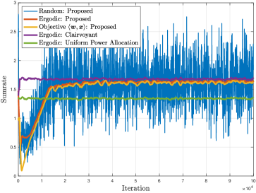
Figure 1: Sumrates achieved by the proposed method, the clairvoyant policy, as well as a deterministic uniform power allocation policy, in the case of a simple AWGN channel.

Key differences between Algorithm 1 and the primal-dual method presented in [33] are the presence of the feasibility slack $\mathtt{S}$, which follows from our analysis, as well as the interesting fact that, due to our explicit formulation of the smoothed surrogate (12), the dual updates (86) and (87) are naturally randomized, in addition to the primal updates (84) and (85). Further, while the model-free algorithm of [33] relies on policy gradient, Algorithm 1 completely bypasses the need for introducing randomized policies into the learning procedure. This also makes Algorithm 1 straightforward to implement, as computation of the gradient of $\boldsymbol{\phi}$ is not required; in fact, Algorithm 1 may be executed as described for any admissible choice of $\boldsymbol{\phi}$, without additional computational requirements.

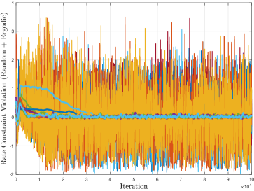
(a)

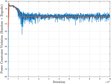
(b)

Figure 2: Rate (left) and power (right) constraint violation exhibited by the proposed method, both random and ergodic, in the case of a simple AWGN channel.

VI Numerical Simulations & Discussion

We now numerically confirm and discuss the efficacy of the proposed primal-dual algorithm (Algorithm 1) by application on two basic wireless models, namely, a classical Additive White Gaussian Noise (AWGN) channel, as well as a Multiple Access Interference (MAI) channel. Also, in all simulations presented in this section, the parameterization $\boldsymbol{\phi}$ is appropriately selected from the well-known $\epsilon$-universal class of fully connected, feed-forward DNNs, with ReLU hidden layers and sigmoid output layers, similar to the setting considered in [33].

For the AWGN channel case, we consider a simple multiuser networking scenario where each user is given a dedicated channel to communicate, with no channel interference. We wish to allocate power between users in order to maximize the weighted sumrate of the network, within a total expected power budget $p_{max}$, provided as a specification. Given fixed and given user priority weights $w^{i}\geq 0,i\in\mathbb{N}_{N_{S}}^{+},$ selected, without loss of generality, such that $\sum_{i}w^{i}\equiv 1$, optimal power allocation may be achieved by solving the stochastic program

$$\begin{array}[]{rl}\underset{x^{i},\boldsymbol{\theta}^{i},i\in\mathbb{N}_{N_{S}}^{+}}{\mathrm{maximize}}&{\displaystyle\sum_{i\in\mathbb{N}_{N_{S}}^{+}}}w^{i}x^{i}\\ \mathrm{subject\,to}&x^{i}\leq{\mathbb{E}}\Bigg{\{}\log\bigg{(}1+\dfrac{H^{i}\phi^{i}(H^{i},\boldsymbol{\theta}^{i})}{\nu^{i}}\bigg{)}\Bigg{\}}\\ &{\mathbb{E}}\Bigg{\{}{\displaystyle\sum_{i\in\mathbb{N}_{N_{S}}^{+}}}\phi^{i}(H^{i},\boldsymbol{\theta}^{i})\Bigg{\}}\leq p_{max}\\ &(x^{i},\boldsymbol{\theta}^{i})\in{\mathbf{R}}_{+}\times{\mathbf{R}}^{N_{\phi^{i}}},\;\forall i\in\mathbb{N}_{N_{S}}^{+}\end{array},$$ (89)

where $H^{i}\geq 0$ and $\nu^{i}>0$ are the fading power and noise variance experienced by the $i$-th user, and each parameterization $\phi^{i}:{\mathbf{R}}_{+}\times{\mathbf{R}}^{N_{\phi^{i}}}\to[0,p_{max}]$ is chosen as a DNN with single input, two hidden layers with eight and four neurons, respectively, and a single output, for all $i\in\mathbb{N}_{N_{S}}^{+}$. The rest of details in regard to the architecture of each of the involved DNNs follows the discussion above. The reason for choosing $N_{S}$ uncoupled DNNs, one for each user, comes from the structure of the globally optimal solution to the most general, unparameterized version of problem (89) (mapping to (1)), which, for this simple networking setting, may be efficiently determined [7]. Of course, this solution results in an ultimate benchmark upper bound of the sumrate achieved by any feasible $\epsilon$-universal resource allocation policy, at the expense of assuming complete knowledge of the true information theoretic description of the communication system; for this reason, we hereafter fairly refer to this solution as clairvoyant.

By defining vectors

$$\boldsymbol{w} \triangleq[w^{1}\,\ldots\,w^{N_{S}}]^{\boldsymbol{T}},$$ (90)

$$\boldsymbol{\phi}({\mathbf{H}},\boldsymbol{\theta}) \triangleq\big{[}\phi^{1}(H^{1},\boldsymbol{\theta}^{1})\,\ldots\,\phi^{N_{S}}(H^{N_{S}},\boldsymbol{\theta}^{N_{S}})\big{]}^{\boldsymbol{T}}\;\text{and}$$ (91)

$$\boldsymbol{\nu} \triangleq\big{[}\nu^{1}\,\ldots\,\nu^{N_{S}}\big{]}^{\boldsymbol{T}},$$ (92)

problem (89) may be reexpressed in the canonical form (2) as

$$\begin{array}[]{rl}\underset{{\mathbf{x}},\boldsymbol{\theta}}{\mathrm{maximize}}&\langle\boldsymbol{w},{\mathbf{x}}\rangle\\ \mathrm{subject\,to}&\begin{bmatrix}{\mathbf{x}}\\ 0\end{bmatrix}\leq{\mathbb{E}}\begin{bmatrix}\log({\bf 1}+{\mathbf{H}}\circ\boldsymbol{\phi}({\mathbf{H}},\boldsymbol{\theta})\varoslash\boldsymbol{\nu})\\ p_{max}-{\bf 1}^{\boldsymbol{T}}\boldsymbol{\phi}({\mathbf{H}},\boldsymbol{\theta})\end{bmatrix}\\ &({\mathbf{x}},\boldsymbol{\theta})\in{\mathbf{R}}_{+}^{N_{S}}\times{\mathbf{R}}^{N_{\boldsymbol{\phi}}}\end{array},$$ (93)

where $\log(\cdot)$ and “$\varoslash$” denote the operations of entrywise logarithm and division, respectively. Therefore, Algorithm 1 is applicable to problem (93) and, in turn, (89), by considering the corresponding smoothed surrogate based on (12).

Since the objective of (89) is usually perfectly known to the wireless engineer, we may set $\mu_{S}\equiv 0$. In other words, in the corresponding smoothed surrogate (cf. (12)), Gaussian smoothing is applied only to the constraints of problem (93).

Remark 17.

Note that, in (89), $H^{i}$ denotes the square of the fading channel experienced by user $i$. Nevertheless, since the square function is one-to-one and onto on the nonnegative reals, taking directly the square of the involved channels is virtually consistent with our setting established in Section I. $\blacksquare$

To assess the performance of the proposed Algorithm 1 on problem (93), we assume $N_{S}\equiv 10$ users, set $p_{max}\equiv 20$, and consider a randomly generated weight vector $\boldsymbol{w}$. We also assume that $\nu^{i}\equiv 1$, and that $H^{i}$ is exponentially distributed with parameter $\lambda\equiv 1/2$, modeling the square of a unit variance Rayleigh fading channel state, for all $i\in\mathbb{N}_{N_{S}}^{+}$. Then, we execute Algorithm 1 for $10^{5}$ iterations, with initial values ${\mathbf{x}}^{0}\equiv{\bf 1},\boldsymbol{\theta}^{0}\equiv{\bf 0}$, $\boldsymbol{\lambda}_{S}^{0}\equiv{\bf 1}_{N_{S}+1}$, constant stepsizes $\boldsymbol{\gamma}_{{\mathbf{x}}}^{n}\equiv 0.001{\bf 1},\boldsymbol{\gamma}_{\boldsymbol{\theta}}^{n}\equiv 0.0008{\bf 1},\boldsymbol{\gamma}_{\boldsymbol{\lambda}_{S}}^{n}\equiv\big{[}0.008{\bf 1}_{N_{S}}^{\boldsymbol{T}}\,0.0001\big{]}^{\boldsymbol{T}}$, for all $n\in\mathbb{N}$, null feasibility slack $\mathtt{S}\equiv{\bf 0}$, and with the smoothing parameter set as $\mu_{R}\equiv 10^{-9}$.

Fig. 1 shows the evolution of the sequence of objective values $\{\langle\boldsymbol{w},{\mathbf{x}}^{n}\rangle\}_{n\in\mathbb{N}}$, the instantaneous sumrate sequence $\{\langle\boldsymbol{w},\log({\bf 1}+{\mathbf{H}}^{n}\circ\hskip 1.0pt\boldsymbol{\phi}({\mathbf{H}}^{n},\boldsymbol{\theta}^{n})\varoslash\hskip 0.5pt\boldsymbol{\nu})\rangle\}_{n\in\mathbb{N}}$, as well as an approximation of the ergodic sumrate sequence $\{\langle\boldsymbol{w},{\mathbb{E}}\{\log({\bf 1}+{\mathbf{H}}\circ\boldsymbol{\phi}({\mathbf{H}},\boldsymbol{\theta}^{n})\varoslash\boldsymbol{\nu})\rangle\}\}_{n\in\mathbb{N}}$. The ergodic performance of Algorithm 1, expressed by the latter estimate, is also compared with the ergodic performance of the unparameterized, globally optimal power allocation policy solving (1) (the clairvoyant), as well as that of a deterministic uniform power allocation policy across users. All ergodic estimates were computed via simple moving average smoothing of the respective process realizations.

Fig. 1 readily demonstrates that the values of the objective of (93) match the values of the estimated ergodic sumrate, as both obtained from Algorithm 1. At the same time, the ergodic sumrate obtained from Algorithm 1 converges remarkably close to that achieved by the clairvoyant policy, which assumes full knowledge of the model describing the wireless system. Therefore, in this case, the proposed zeroth-order primal-dual method attains actually near-optimal system performance.

Fig. 2 shows similar type estimates (instantaneous and ergodic) concerning violation of the rate and power constraints of problem (93), during execution of Algorithm 1 (positive values indicate constraint violation). We observe that all constraints are active (i.e., met with equality) on average, which confirms that the proposed primal-dual-method indeed converges to feasible power allocation policies, while achieving maximal ergodic rates on a per user basis, as desired. We emphasize that, contrary to the clairvoyant solution, such good performance of Algorithm 1 is achieved without the availability of a baseline model of the wireless system, and at the absence of gradient information of information rate functions, as well as DNN parameterizations.

Next, we consider the case of a MAI channel, where $N_{S}$ transmitters simultaneously communicate with a central node, for instance, a common receiver, or a base station. In this case, the signal transmitted by each user creates interference to the signals transmitted by all other users in the network. As before, we would like to optimally allocate power between users in order to maximize the weighted sumrate of the network, within a total expected power specification $p_{max}$. Working similarly to the AWGN channel case discussed above, we may formulate the stochastic program

$$\begin{array}[]{rl}\underset{x^{i},i\in\mathbb{N}_{N_{S}}^{+},\boldsymbol{\theta}}{\mathrm{maximize}}&{\displaystyle\sum_{i\in\mathbb{N}_{N_{S}}^{+}}}w^{i}x^{i}\\ \mathrm{subject\,to}&x^{i}\leq{\mathbb{E}}\Bigg{\{}\log\Bigg{(}1+\dfrac{H^{i}\phi^{i}({\mathbf{H}},\boldsymbol{\theta})}{\nu^{i}+\sum_{i\neq j}H^{j}\phi^{j}({\mathbf{H}},\boldsymbol{\theta})}\Bigg{)}\Bigg{\}}\\ &{\mathbb{E}}\Bigg{\{}{\displaystyle\sum_{i\in\mathbb{N}_{N_{S}}^{+}}}\phi^{i}({\mathbf{H}},\boldsymbol{\theta})\Bigg{\}}\leq p_{max}\\ &(x^{i},\boldsymbol{\theta})\in{\mathbf{R}}_{+}\times{\mathbf{R}}^{N_{\boldsymbol{\phi}}},\;\forall i\in\mathbb{N}_{N_{S}}^{+}\end{array},$$ (94)

where each parameterization $\phi^{i}:{\mathbf{R}}_{+}^{N_{S}}\times{\mathbf{R}}^{N_{\boldsymbol{\phi}}}\to[0,p_{max}]$, $i\in\mathbb{N}_{N_{S}}^{+}$ is an element of the output layer of a single DNN taking as input the full fading channel vector ${\mathbf{H}}\in{\mathbf{R}}_{+}^{N_{S}}$, and having two hidden layers with thirty-two and sixteen neurons, respectively. The intuition behind the adopted multiple-input multiple-output DNN architecture lies in the strong coupling among the channels of all users in every rate constraint of (94). The rest of details in regard to the architecture of each of the involved DNNs follows the discussion above.

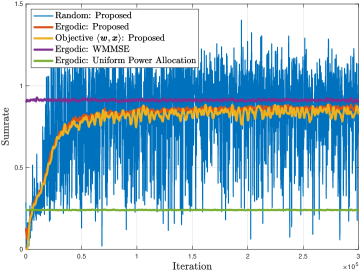
Figure 3: Sumrates achieved by the proposed method, the WMMSE policy, and a deterministic uniform power allocation policy, in the case of a MAI channel.

As before, problem (94) may be reexpressed in the form of (2); however, the details are slightly more technical compared to the case of an AWGN channel, and are omitted for brevity.

In our simulations for this setting, we assume $N_{S}\equiv 5$ users, a power budget $p_{max}\equiv 20$, and a randomly generated weight vector $\boldsymbol{w}$. We also let $\nu^{i}\equiv 1$, and $H^{i}$ follows the same exponential distribution as before, for all $i\in\mathbb{N}_{N_{S}}^{+}$. Then, we execute Algorithm 1 for $3\cdot 10^{5}$ iterations, with initial values ${\mathbf{x}}^{0}\equiv\boldsymbol{\theta}^{0}\equiv{\bf 0}$, $\boldsymbol{\lambda}_{S}^{0}\equiv{\bf 1}_{N_{S}+1}$, constant stepsizes $\boldsymbol{\gamma}_{{\mathbf{x}}}^{n}\equiv 0.0008{\bf 1},\boldsymbol{\gamma}_{\boldsymbol{\theta}}^{n}\equiv 0.0005{\bf 1},\boldsymbol{\gamma}_{\boldsymbol{\lambda}_{S}}^{n}\equiv\big{[}0.005{\bf 1}_{N_{S}}^{\boldsymbol{T}}\,0.0001\big{]}^{\boldsymbol{T}}$, for all $n\in\mathbb{N}$, null feasibility slack $\mathtt{S}\equiv{\bf 0}$, and with the smoothing parameter set as $\mu_{R}\equiv 10^{-9}$. As before, we set $\mu_{R}\equiv 0$, that is, the objective of (94) is reasonable assumed known.

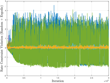
(a)

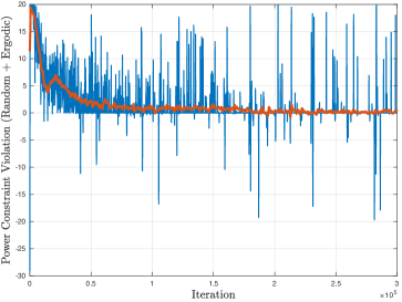
(b)

Figure 4: Rate (left) and power (right) constraint violation exhibited by the proposed method, both random and ergodic, in the case of a MAI channel.

Fig. 3 shows the evolution of the sequence of objective values $\{\langle\boldsymbol{w},{\mathbf{x}}^{n}\rangle\}_{n\in\mathbb{N}}$ and, as before, the instantaneous sumrate sequence obtained from Algorithm 1, as well as an approximation of the corresponding ergodic sumrate. Since the solution to the variational version of (94) is unavailable mainly due to nonconvexity of the involved rate constraints (cf. (1)), we compare the ergodic performance of Algorithm 1 with that of the well-known WMMSE policy [15], which is an iterative algorithm providing an approximate solution, for each fading realization, to the deterministic sumrate maximization problem

$$\begin{array}[]{rl}\underset{p^{i},i\in\mathbb{N}_{N_{S}}^{+}}{\mathrm{maximize}}&{\displaystyle\sum_{i\in\mathbb{N}_{N_{S}}^{+}}}w^{i}\log\bigg{(}1+\dfrac{H^{i}p^{i}}{\nu^{i}+\sum_{i\neq j}H^{j}p^{j}}\bigg{)}\\ \mathrm{subject\,to}&{\displaystyle\sum_{i\in\mathbb{N}_{N_{S}}^{+}}}p^{i}\leq p_{max}\\ &p^{i}\geq 0,\;\forall i\in\mathbb{N}_{N_{S}}^{+}\end{array},$$ (95)

Additionally, note that, as the form of problem (95) suggests, the WMMSE heuristic assumes complete knowledge of the information theoretic model of the wireless system. For reference, Fig. 3 also shows the ergodic performance achieved by a uniform power allocation policy across users. As before, all ergodic estimates were computed via simple moving average smoothing of the respective process realizations.

Fig. 3 confirms that Algorithm 1 exhibits similar behavior as in the AWGN channel case previously discussed, but for the significantly more complicated resource allocation problem (94). Again, the objective of (94) and the ergodic sumrate obtained from Algorithm 1 match, whereas the latter converges rather close to the ergodic sumrate achieved by WMMSE.

Instantaneous and ergodic estimates of the rate and power constraint violation of the decisions produced by Algorithm 1 for problem (94) are provided in Fig. 4 (again, positive values indicate constraint violation). As in the AWGN channel case, all constraints are active on average, confirming that the proposed zeroth-order primal-dual method produces feasible and near-state-of-the-art power allocation policies without knowledge of a system model and in absence of gradient information, verifying the effectiveness of the method in a model-agnostic setting.

VII Conclusion

We have considered the general problem of learning optimal resource allocation policies in wireless systems, under a model-free, data-driven setting. Starting with a generic variational formulation of the resource allocation problem, and driven by its intractability in most wireless networking scenarios, we focused on parametric policy function approximations. Leveraging classical results on Gaussian smoothing, we first showed that it is possible to crucially simplify gradient evaluation for all utility and service functions involved, by appropriately constructing a finite dimensional, smoothed surrogate to the original variational problem. Then, assuming near-universal policy parameterizations, e.g., Deep Neural Networks (DNNs), we completely characterized the duality gap between the original problem and the dual of the proposed surrogate, establishing linear dependence of this duality gap relative to smoothing and near-universality parameters. In fact, this gap may be made arbitrarily small at will. Motivated by our results, and in conjunction with the special properties of the proposed smoothed surrogate, we also developed a zeroth-order stochastic primal-dual algorithm, enabling completely model-free, data-driven optimal resource allocation for ergodic network optimization. Our simulations show that DNN-based, data-driven policies produced by the proposed primal-dual method attain near-ideal performance, relying exclusively on limited system probing, completely bypassing the need for gradient computations and policy randomization, and at the absence of baseline channel or information rate models.

References

- [1] A. Ribeiro, “Optimal resource allocation in wireless communication and networking,” EURASIP Journal on Wireless Communications and Networking, vol. 2012, no. 1, p. 272, 2012.
- [2] Wei Yu and R. Lui, “Dual methods for nonconvex spectrum optimization of multicarrier systems,” IEEE Transactions on Communications, vol. 54, no. 7, pp. 1310–1322, Jul. 2006.
- [3] C. S. Chen, K. W. Shum, and C. W. Sung, “Round-robin power control for the weighted sumrate maximisation of wireless networks over multiple interfering links,” European Transactions on Telecommunications, vol. 22, no. 8, pp. 458–470, Dec. 2011.
- [4] N. Naderializadeh and A. S. Avestimehr, “Itlinq: A new approach for spectrum sharing in device-to-device communication systems,” IEEE Journal on Selected Areas in Communications, vol. 32, no. 6, pp. 1139–1151, Jun. 2014.
- [5] J. Zhang and D. Zheng, “A stochastic primal-dual algorithm for joint flow control and mac design in multi-hop wireless networks,” in 2006 40th Annual Conference on Information Sciences and Systems. IEEE, Mar. 2006, pp. 339–344.
- [6] X. Wu, S. Tavildar, S. Shakkottai, T. Richardson, J. Li, R. Laroia, and A. Jovicic, “Flashlinq: A synchronous distributed scheduler for peer-to-peer ad hoc networks,” IEEE/ACM Transactions on Networking, vol. 21, no. 4, pp. 1215–1228, Aug. 2013.
- [7] X. Wang and N. Gao, “Stochastic resource allocation over fading multiple access and broadcast channels,” IEEE Transactions on Information Theory, vol. 56, no. 5, pp. 2382–2391, May 2010.
- [8] J. Rubio, O. Muñoz-Medina, A. Pascual-Iserte, and J. Vidal, “Stochastic resource allocation with a backhaul constraint for the uplink,” in IEEE International Symposium on Personal, Indoor and Mobile Radio Communications, PIMRC. IEEE, Sep. 2016, pp. 1–6.
- [9] Yichuan Hu and A. Ribeiro, “Adaptive distributed algorithms for optimal random access channels,” IEEE Transactions on Wireless Communications, vol. 10, no. 8, pp. 2703–2715, Aug. 2011.
- [10] Y. Hu and A. Ribeiro, “Optimal wireless networks based on local channel state information,” IEEE Transactions on Signal Processing, vol. 60, no. 9, pp. 4913–4929, Sep. 2012.
- [11] X. Wang and G. B. Giannakis, “Resource allocation for wireless multiuser ofdm networks,” IEEE Transactions on Information Theory, vol. 57, no. 7, pp. 4359–4372, Jul. 2011.
- [12] D. Wang, Z. Li, and X. Wang, “Joint optimal subcarrier and power allocation for wireless cooperative networks over ofdm fading channels,” in IEEE Transactions on Vehicular Technology, vol. 61, no. 1, Jan. 2012, pp. 249–257.
- [13] T. He, X. Wang, and W. Ni, “Optimal chunk-based resource allocation for ofdma systems with multiple ber requirements,” IEEE Transactions on Vehicular Technology, vol. 63, no. 9, pp. 4292–4301, Nov. 2014.
- [14] H. Yu and M. J. Neely, “Dynamic transmit covariance design in mimo fading systems with unknown channel distributions and inaccurate channel state information,” IEEE Transactions on Wireless Communications, vol. 16, no. 6, pp. 3996–4008, Jun. 2017.
- [15] Q. Shi, M. Razaviyayn, Z.-Q. Luo, and C. He, “An iteratively weighted mmse approach to distributed sum-utility maximization for a mimo interfering broadcast channel,” IEEE Transactions on Signal Processing, vol. 59, no. 9, pp. 4331–4340, Sep. 2011.
- [16] N. Sidiropoulos, T. Davidson, and Zhi-Quan Luo, “Transmit beamforming for physical-layer multicasting,” IEEE Transactions on Signal Processing, vol. 54, no. 6, pp. 2239–2251, Jun. 2006.
- [17] J.-A. Bazerque and G. B. Giannakis, “Distributed scheduling and resource allocation for cognitive ofdma radios,” in 2007 2nd International Conference on Cognitive Radio Oriented Wireless Networks and Communications. IEEE, Aug. 2007, pp. 343–350.
- [18] A. S. Bedi and K. Rajawat, “Asynchronous incremental stochastic dual descent algorithm for network resource allocation,” IEEE Transactions on Signal Processing, vol. 66, no. 9, pp. 2229–2244, May 2018.
- [19] ——, “Network resource allocation via stochastic subgradient descent: Convergence rate,” IEEE Transactions on Communications, vol. 66, no. 5, pp. 2107–2121, May 2018.
- [20] K. Gatsis, M. Pajic, A. Ribeiro, and G. J. Pappas, “Opportunistic control over shared wireless channels,” IEEE Transactions on Automatic Control, vol. 60, no. 12, pp. 3140–3155, Dec. 2015.
- [21] M. Eisen, K. Gatsis, G. J. Pappas, and A. Ribeiro, “Learning in wireless control systems over nonstationary channels,” IEEE Transactions on Signal Processing, vol. 67, no. 5, pp. 1123–1137, Mar. 2019.
- [22] K. Gatsis, A. Ribeiro, and G. J. Pappas, “Random access design for wireless control systems,” Automatica, vol. 91, pp. 1–9, May 2018.
- [23] T. Van Chien, E. Björnson, and E. G. Larsson, “Sum spectral efficiency maximization in massive mimo systems: Benefits from deep learning,” arXiv preprint, arXiv:1903.08163, Mar. 2019.
- [24] D. Xu, X. Che, C. Wu, S. Zhang, S. Xu, and S. Cao, “Energy-efficient subchannel and power allocation for hetnets based on convolutional neural network,” arXiv preprint, arXiv:1903.00165, Mar. 2019.
- [25] L. Lei, L. You, G. Dai, T. X. Vu, D. Yuan, and S. Chatzinotas, “A deep learning approach for optimizing content delivering in cache-enabled hetnet,” in 2017 International Symposium on Wireless Communication Systems (ISWCS). IEEE, Aug. 2017, pp. 449–453.
- [26] H. Sun, X. Chen, Q. Shi, M. Hong, X. Fu, and N. D. Sidiropoulos, “Learning to optimize: Training deep neural networks for interference management,” IEEE Transactions on Signal Processing, vol. 66, no. 20, pp. 5438–5453, Oct. 2018.
- [27] W. Lee, M. Kim, and D.-H. Cho, “Deep power control: Transmit power control scheme based on convolutional neural network,” IEEE Communications Letters, vol. 22, no. 6, pp. 1276–1279, Jun. 2018.
- [28] P. de Kerret, D. Gesbert, and M. Filippone, “Team deep neural networks for interference channels,” in 2018 IEEE International Conference on Communications Workshops (ICC Workshops). IEEE, May 2018, pp. 1–6.
- [29] F. Liang, C. Shen, W. Yu, and F. Wu, “Towards optimal power control via ensembling deep neural networks,” arXiv preprint, arXiv:1807.10025, Jul. 2018.
- [30] W. Cui, K. Shen, and W. Yu, “Spatial deep learning for wireless scheduling,” IEEE Journal on Selected Areas in Communications, vol. 37, no. 6, pp. 1248–1261, Dec. 2019.
- [31] Z. Xu, Y. Wang, J. Tang, J. Wang, and M. C. Gursoy, “A deep reinforcement learning-based framework for power-efficient resource allocation in cloud rans,” in 2017 IEEE International Conference on Communications (ICC). IEEE, May 2017, pp. 1–6.
- [32] F. Meng, P. Chen, L. Wu, and J. Cheng, “Power allocation in multi-user cellular networks: Deep reinforcement learning approaches,” arXiv preprint, arXiv:1901.07159, Jan. 2019.
- [33] M. Eisen, C. Zhang, L. F. Chamon, D. D. Lee, and A. Ribeiro, “Learning optimal resource allocations in wireless systems,” IEEE Transactions on Signal Processing, vol. 67, no. 10, pp. 2775–2790, May 2019.
- [34] M. Eisen and A. Ribeiro, “Optimal wireless resource allocation with random edge graph neural networks,” arXiv preprint, arXiv:1909.01865, Sep. 2019.
- [35] W. B. Powell, “A unified framework for stochastic optimization,” pp. 795–821, Jun. 2019. [Online]. Available: https://www.sciencedirect.com/science/article/abs/pii/S0377221718306192
- [36] J. Park and I. W. Sandberg, “Universal approximation using radial-basis-function networks,” Neural Computation, vol. 3, no. 2, pp. 246–257, Jun. 1991.
- [37] B. K. Sriperumbudur, K. Fukumizu, and G. R. G. Lanckriet, “On the relation between universality , characteristic kernels and rkhs embedding of measures,” in 13th Intern. Conf. Artificial Intelligence and Statistics, no. 9, Mar. 2010, pp. 773–780.
- [38] K. Hornik, M. Stinchcombe, and H. White, “Multilayer feedforward networks are universal approximators,” Neural Networks, vol. 2, no. 5, pp. 359–366, 1989.
- [39] W. B. Powell, Approximate Dynamic Programming: Solving the Curses of Dimensionality, 2nd ed. Wiley-Interscience, 2011.
- [40] D. Bertsekas, Dynamic Programming & Optimal Control, 4th ed. Belmont, Massachusetts: Athena Scientific, 2012, vol. II.
- [41] R. S. Sutton and A. G. Barto, Reinforcement Learning: An Introduction, 2nd ed. MIT Press, 2018.
- [42] H. J. H. J. Kushner and G. Yin, Stochastic Approximation and Recursive Algorithms and Applications. Springer, 2003.
- [43] J. C. Spall, Introduction to Stochastic Search and Optimization: Estimation, Simulation, and Control. Wiley-Interscience, 2003.
- [44] Y. Nesterov and V. Spokoiny, “Random gradient-free minimization of convex functions,” Foundations of Computational Mathematics, vol. 17, no. 2, pp. 527–566, Apr. 2017.
- [45] R. B. Ash and C. Doléans-Dade, Probability and Measure Theory. Academic Press, 2000.
- [46] S. P. Boyd and L. Vandenberghe, Convex Optimization. Cambridge University Press, 2004.
- [47] A. P. Ruszczyński, Nonlinear Optimization. Princeton University Press, 2006.
- [48] D. P. Bertsekas, Convex optimization theory, 1st ed. Athena Scientific, 2009.