A unified approach for projections onto the intersection of $\ell_{1}$ and $\ell_{2}$ balls or spheres

Abstract

This paper focuses on designing a unified approach for computing the projection onto the intersection of an $\ell_{1}$ ball/sphere and an $\ell_{2}$ ball/sphere. We show that the major computational efforts of solving these problems all rely on finding the root of the same piecewisely quadratic function, and then propose a unified numerical method to compute the root. In particular, we design breakpoint search methods with/without sorting incorporated with bisection, secant and Newton methods to find the interval containing the root, on which the root has a closed form. It can be shown that our proposed algorithms without sorting possess $O(n\log n)$ worst-case complexity and $O(n)$ in practice. The efficiency of our proposed algorithms are demonstrated in numerical experiments.

Keywords: projection , intersection , $\ell_{1}$ ball, breakpoint search, principle component analysis

1 Introduction

In this paper, we consider designing a unified numerical method for computing the solution of the following three types of problems: projection onto the intersection of an $\ell_{1}$ ball and an $\ell_{2}$ ball:

$$\mathop{\rm minimize}\limits_{{\bm{x}}\in{\mathbb{R}}^{n}}\tfrac{1}{2}\|{\bm{x}}-{\bm{v}}\|_{2}^{2}\quad{\rm subject\ to}\ {\bm{x}}\in\mathbb{B}_{1}^{t}\cap\mathbb{B}_{2},$$ (1.1)

projection onto the intersection of an $\ell_{1}$ ball and an $\ell_{2}$ sphere:

$$\mathop{\rm minimize}\limits_{{\bm{x}}\in{\mathbb{R}}^{n}}\tfrac{1}{2}\|{\bm{x}}-{\bm{v}}\|_{2}^{2}\quad{\rm subject\ to}\ {\bm{x}}\in\mathbb{B}_{1}^{t}\cap\mathbb{S}_{2},$$ (1.2)

and projection onto the intersection of an $\ell_{1}$ sphere and an $\ell_{2}$ sphere:

$$\mathop{\rm minimize}\limits_{{\bm{x}}\in{\mathbb{R}}^{n}}\tfrac{1}{2}\|{\bm{x}}-{\bm{v}}\|_{2}^{2}\quad{\rm subject\ to}\ {\bm{x}}\in\mathbb{S}_{1}^{t}\cap\mathbb{S}_{2}.$$ (1.3)

Here the $\ell_{2}$ (i.e., Euclidean) norm on ${\mathbb{R}}^{n}$ is indicated as $\|\cdot\|_{2}$ with the unit $\ell_{2}$ ball (sphere) defined as ${\mathbb{B}}_{2}:=\{{\bm{x}}\in{\mathbb{R}}^{n}:\|{\bm{x}}\|_{2}\leq 1\}$ $(\mathbb{S}_{2}=\{{\bm{x}}\in{\mathbb{R}}^{n}:\|{\bm{x}}\|_{2}=1\}$), and the $\ell_{1}$ norm is indicated as $\|\cdot\|_{1}$ with the $\ell_{1}$ ball (sphere) with radius $t$ denoted as ${\mathbb{B}}_{1}^{t}:=\{{\bm{x}}\in{\mathbb{R}}^{n}:\|{\bm{x}}\|_{1}\leq t\}$ ($\mathbb{S}_{1}^{t}=\{{\bm{x}}\in{\mathbb{R}}^{n}:\|{\bm{x}}\|_{1}=t\}$). Notice that $\|x\|_{2}\leq\|x\|_{1}\leq\sqrt{n}\|x\|_{2}$. Trivial cases for the problems of interests are: (a) $t\leq 1$, in this case $\|x\|_{1}\leq t$ implies $\|x\|_{2}<1$, meaning ${\mathbb{B}}_{1}^{t}\subset{\mathbb{B}}_{2}$, $\mathbb{S}_{1}^{t}\cap{\mathbb{B}}_{2}=\emptyset$ and $\mathbb{S}_{1}^{t}\cap\mathbb{S}_{2}=\emptyset$. (b) $t\geq\sqrt{n}$, in this case $\|x\|_{2}\leq 1$ implies $\|x\|_{1}<t$, meaning ${\mathbb{B}}_{2}\subset{\mathbb{B}}_{1}^{t}$, $\mathbb{S}_{1}^{t}\cap{\mathbb{B}}_{2}=\emptyset$ and $\mathbb{S}_{1}^{t}\cap\mathbb{S}_{2}=\emptyset$. Without loss of generality, we assume $1\leq t\leq\sqrt{n}$ in the remainder of this paper.

Problems (1.1) (1.2) and (1.3) arise widely in modern science, engineering and business. For example, the gradient projection methods for Sparse Principal Component Analysis (sPCA)[1, 2, 3, 4] often involve problems of (1.1) or (1.3), and (1.3) is also an integral part in efficient sparse non-negative matrix factorization [6, 7], supervised online autoencoder intended for classification using neural networks that features sparse activity and sparse connectivity [8], and dictionary learning with sparseness-enforcing projections [8]. Problem (1.2) often arises in Sparse Generalized Canonical Correlation Analysis (SGCCA)[5], and Witten et al. [4] use (1.2) for computing the rank-1 approximation for a given matrix along with a block coordinate decent method, which can be applied to sparse principal components and canonical correlation.

Our contribution in this paper can be summarized as follows:

• We propose a unified analysis for solving these problems. Specifically, we show that their solutions can all be determined by the root of a piecewisely quadratic auxiliary function.

• A series of properties of the proposed auxiliary function are provided, which provide detailed characterization of the solutions of these problems.

• A unified method with/without sorting is designed for finding the root of the auxiliary function, which accounts for the major computational efforts of solving these problems.

1.1 Organization

In the remainder of this section, we outline our notation and introduce various concepts that will be employed throughout the paper. In §2, we discuss the most related existing problems and algorithms. In §3, we introduce our proposed auxiliary function and provide a series of properties of the auxiliary function. We use the proposed auxiliary function to characterize the optimal solutions in §4. A unified algorithm is proposed in §5 for finding the root of the auxiliary function. The results of numerical results are shown in §6. Concluding remarks are provided in §7.

1.2 Notation

For any ${\bm{x}}\in{\mathbb{R}}^{n}$, let $x_{i}$ be the $i$-th element of ${\bm{x}}$ and ${\mathbb{R}}^{n}_{+}$ be the nonnegative orthant of ${\mathbb{R}}^{n}$, i.e., ${\mathbb{R}}^{n}_{+}:=\{{\bm{x}}\in{\mathbb{R}}^{n}:x_{i}\geq 0,i=1,\ldots,n\}$. Denote the soft thresholding operator in ${\mathbb{R}}^{n}$ with threshold $\lambda>0$ by $S_{\lambda}(\cdot)$, i.e., for any ${\bm{x}}\in{\mathbb{R}}^{n}$, $(S_{\lambda}({\bm{x}}))_{i}={\rm sign}(x_{i})\max(|x_{i}|-\lambda)$ for $i=1,\ldots,n$. Given ${\bm{v}}\in\mathbb{R}^{n}$, denote ${\bm{v}}^{+}$ as the projection of ${\bm{v}}$ onto the nonnegative orthant $\mathbb{R}^{n}_{+}$, i.e. ${\bm{v}}^{+}=\max({\bm{v}},0)$. The $\ell_{p,q}$ norm of ${\bm{x}}$ is defined as $\|{\bm{x}}\|_{p,q}=\left(\sum_{i=1}^{G}\|{\bm{x}}_{i}\|_{q}^{p}\right)^{1/p}$ with ${\bm{x}}_{i}\in\mathbb{R}^{n_{i}}$ and $\sum_{i=1}^{G}n_{i}=n$, where $G$ is the number of groups. For a compact set $\Omega\subset\mathbb{R}^{n}$ and ${\bm{v}}\in\mathbb{R}^{n}$, denote $\text{proj}_{\Omega}({\bm{v}})=\arg\min_{{\bm{x}}\in\mathbb{R}^{n}}\|{\bm{v}}-{\bm{x}}\|_{2}^{2}$. The function $\phi:\mathbb{R}^{n}\to\bar{\mathbb{R}}:=\mathbb{R}\cup\{+\infty\}$ is convex, then the subdifferential of $\phi$ at $\bar{\bm{x}}$ is given by $\partial\phi(\bar{\bm{x}}):=\{{\bm{z}}\in{\mathbb{R}}^{n}\mid\phi(\bar{\bm{x}})+{\bm{z}}^{T}({\bm{x}}-\bar{\bm{x}})\leq\phi({\bm{x}}),\forall{\bm{x}}\in\mathbb{R}^{n}\}.$

Denote ${\bf 1}\in{\mathbb{R}}^{n}$ be the vector of all ones. The largest and the second-largest of ${\bm{v}}$ are denoted as $v_{\max}=\max(v_{1},...,v_{n})$ and $v_{\text{2nd-max}}$, respectively. To simplify the analysis, we assume $\lambda_{j},j=1,\ldots,k$ are the $k$ distinct components of ${\bm{v}}$ such that $\lambda_{1}>\ldots>\lambda_{k}$ with $\lambda_{1}=v_{\max}$ and $\lambda_{k+1}=-\infty$.

2 Related methods

We discuss the most related works in this section.

Projection onto $\ell_{1}$ ball. As for projection onto a single $\ell_{1}$ ball, many algorithms have emerged. It can be shown [9, 10, 11] that the projection of ${\bm{v}}$ onto $\mathbb{B}_{1}^{t}$ can be characterized by the root of the auxiliary function

$$\psi(\lambda):=\sum_{i=1}^{n}\max(v_{i}-\lambda,0)-t=\|({\bm{v}}-\lambda\bm{1})^{+}\|_{1}-t.$$

The properties of $\psi$ are summarized in the proposition below.

Proposition 2.1.

Function $\psi$ is continuous, strictly decreasing and piecewisely linear on $(-\infty,v_{\max}]$ with breakpoints $\lambda_{1},\ldots,\lambda_{k}$, and $\psi\equiv-t<0$ for any $\lambda\geq v_{\max}$.

By Proposition 2.1, $\psi(\lambda)=0$ has a unique root on $(-\infty,v_{\max})$ since $\psi(\lambda)\to+\infty$ as $\lambda\to-\infty$ and $\psi(v_{\max})=-t<0$. The algorithms for computing the $\ell_{1}$ ball projection are summarized and compared in [12], in which an efficient algorithm is also proposed with worst-case complexity $O(n^{2})$ and observed complexity $O(n)$.

Group ball projection. The first related work is the Euclidean projection onto the intersection of $\ell_{1}$ and $\ell_{1,q}$ norm balls ($q=2$ or $q=\infty$) proposed by Su et al. [13]. With $q=2$ and one group, this problem reverts to (1.1). They proved that the projection can be reduced to finding the root of an auxiliary function

$$\phi_{1}(\lambda):=\|S_{\lambda}({\bm{v}})\|_{1}/\|S_{\lambda}({\bm{v}})\|_{2}-t,\quad\lambda\in[0,v_{\max}).$$

Su et al. [13] studied the properties of this auxiliary function, which are summarized in the following Lemma 2.2. Based on this lemma, a bisection algorithm is proposed to find the root of $\phi_{1}$.

Lemma 2.2 ([13] Theorem 1).

The following statements hold true: (i) $\phi_{1}$ is continuous piece-wise smooth on $(0,v_{\max})$; (ii) $\phi_{1}$ is monotonically decreasing and has a unique root in $(0,v_{\max})$.

Remark: However, part (ii) of this lemma may not hold in general. We show this by the following two counterexamples.

Example 1. Consider $n=2,t=1.2$ and ${\bm{v}}=(1,0)$. Then for $\lambda\in(0,1)$

$$\phi_{1}(\lambda)=\frac{\max(1-\lambda,0)+\max(-\lambda,0)}{\sqrt{(\max(1-\lambda,0))^{2}+(\max(-\lambda,0))^{2}}}-1.2=-0.2.$$

Obviously, for this instance, $\phi_{1}$ has no root on $(0,1)$. Therefore, Lemma 2.2 does not hold.

Example 2. Consider $n=3,t=\sqrt{2}$ and ${\bm{v}}=(1,1,0)$. Then for $\lambda\in(0,1)$

$$\phi_{1}(\lambda)=\frac{2\max(1-\lambda,0)+\max(-\lambda,0)}{\sqrt{2(\max(1-\lambda,0))^{2}+(\max(-\lambda,0))^{2}}}-\sqrt{2}\equiv 0.$$

Clearly, any point in $(0,1)$ is the root of $\phi_{1}$, so that Lemma 2.2 does not hold.

Sparseness-enforcing projection operator. Another related work is the “sparseness-enforcing projection operator” proposed by Hoyer [6], which requires the solution to satisfy a normalized smooth “sparseness measure” defined by

$$\sigma:{\mathbb{R}}^{n}\setminus\{0\}\to[0,1],\ {\bm{v}}\mapsto(\sqrt{n}-\|{\bm{v}}\|_{1}/\|{\bm{v}}\|_{2})/(\sqrt{n}-1).$$

This leads to solving the problem of (1.3).

Theis et al. [14] shown that the projection is almost surely unique for ${\bm{v}}$ drawn from a continuous distribution, and if it is unique, the projection is shown to be determined by the root of $\phi_{1}$. We summarized the results in Lemma 2.3. Algorithms for solving (1.3) mainly include the alternating projection method in [6, 14], the method of Lagrange multipliers based on sorted ${\bm{v}}$ in [7], and the method in [8] based on computing the root of the auxiliary function $\phi_{1}(\lambda)$.

Lemma 2.3.

([8, Lemma 3 in Appendix]) Let ${\bm{v}}\in\mathbb{R}^{n}_{+}\setminus{\mathbb{R}^{n}_{+}\cap\mathbb{S}^{t}_{1}\cap\mathbb{S}_{2}}$ be a point such that ${\rm proj}_{\mathbb{R}^{n}_{+}\cap\mathbb{S}^{t}_{1}\cap\mathbb{S}_{2}}({\bm{v}})$ is unique and $\sigma({\bm{v}})<\sigma^{*}$. Then $\phi_{1}$ is well defined and the following hold:

1. $\phi_{1}$ is continuous on $(0,v_{\max})$;

2. $\phi_{1}$ is differentiable on $(0,v_{\max})\setminus\{v_{1},\ldots,v_{n}\}$.

3. $\phi_{1}$ is strictly decreasing on $(0,v_{\rm 2nd-max})$, and is constant on $[v_{\rm 2nd-max},v_{\max})$.

4. $\phi_{1}$ has a unique root $\alpha^{*}\in(0,v_{\rm 2nd-max})$, and ${\rm proj}_{\mathbb{R}^{n}_{+}\cap\mathbb{S}^{t}_{1}\cap\mathbb{S}_{2}}({\bm{v}})=\frac{S_{\alpha^{*}}({\bm{v}})}{\|S_{\alpha^{*}}({\bm{v}})\|_{2}}$.

Remark: Here the condition $\sigma({\bm{v}})<\sigma^{*}$ holds if and only $\|{\bm{v}}^{+}\|_{1}>t\|{\bm{v}}^{+}\|_{2}$. Compared with Theorem 4.3, Lemma 2.3 may not include the situation where the projection is not unique or the projection is unique but $\sigma({\bm{v}})\geq\sigma^{*}$.

Projection onto intersection of an $\ell_{1}$ ball and an $\ell_{2}$ sphere. Tenenhaus et al. [5] provided a close form of the solution (1.2). The algorithms for solving (1.2) mainly include the root finding with bisection proposed by [5] and the root finding method with sorting ${\bm{v}}$ by [15]. Let $\tilde{\bm{v}}=|{\bm{v}}|$ and suppose the elements are sorted in descent order. They analyzed the properties of $\phi_{1}(\lambda)$ in the following lemma.

Lemma 2.4.

([15, Proposition 1]) The following statements hold true.

• $\phi_{1}$ is continuous and decreasing.

• Let $n_{\max}$ be the number of elements of ${\bm{v}}$ equal to $v_{\max}$. For $t\in[\sqrt{n_{\max}},\sqrt{n}]$, there exists $i\in\{1,\ldots,n\}$ and $\delta\in[0,\tilde{v}_{i}-\tilde{v}_{i+1})$ such that $\phi_{1}(\tilde{v}_{i}-\delta)=0$.

• $\delta$ is a solution of a second degree polynomial equation.

Remark. Part (ii) of Lemma 2.4 shown that $n_{\max}\leq t^{2}$ is the sufficient condition that $\phi_{1}(\lambda)=0$ have a root on $(0,\tilde{v}_{\max})$. However, Example 1 is a counterexample indicating that $n_{\max}\leq t^{2}$ is not sufficient to guarantee $\phi_{1}(\lambda)$ has a root on $(0,v_{\max})$.

3 Proposed auxiliary function

Based on the discussion in §2, most existing projection algorithms onto the intersection of $\ell_{1}$ and $\ell_{2}$ balls/spheres are constructed by using the auxiliary function $\phi_{1}(\lambda)$. Our proposed methods are based on different auxiliary functions for characterizing the properties of the projections, which is the main focus of this section.

We first show that the solutions of (1.1)/(1.2)/(1.3), have the same sign as the given ${\bm{v}}$, which is a generalized result of the $\ell_{1}$ ball projection in [9, 16].

Proposition 3.1.

Let ${\bm{x}}$ be the first-order optimal to (1.1)/(1.2)/(1.3), then $v_{i}x_{i}\geq 0$ for $i=1,\ldots,n$.

Proof.

Assume by contradiction that there exists $i_{0}$ such that $v_{i_{0}}x_{i_{0}}<0$. Define $\hat{\bm{x}}$ such that $\hat{x}_{i_{0}}=-x_{i_{0}}$ and $\hat{x}_{i}=x_{i}$ for all $i\neq i_{0}$, implying $\|\hat{\bm{x}}\|_{p}=\|{\bm{x}}\|_{p},p=1,2$. Therefore, $\hat{\bm{x}}$ is feasible for (1.1)/(1.2)/(1.3). However,

$$\tfrac{1}{2}(\|{\bm{x}}-{\bm{v}}\|_{2}^{2}-\|\hat{\bm{x}}-{\bm{v}}\|_{2}^{2})=\tfrac{1}{2}((x_{i_{0}}-v_{i_{0}})^{2}-(-x_{i_{0}}-v_{i_{0}})^{2})=-2v_{i_{0}}x_{i_{0}}>0,$$

contradicting that ${\bm{x}}$ is optimal for (1.1)/(1.2)/(1.3). This completes the proof. ∎

Using the symmetry of the feasible region stated in Proposition 3.1, we can transform the original problems (1.1), (1.2) and (1.3) to their corresponding problems restricted in $\mathbb{R}^{n}_{+}$, so that from now on we can focus on the following problems

$$\mathop{\rm minimize}\limits_{{\bm{x}}}\tfrac{1}{2}\|{\bm{x}}-{\bm{v}}\|_{2}^{2}\quad{\rm subject\ to}\ {\bm{x}}\in\mathbb{B}_{1}^{t}\cap\mathbb{B}_{2}\cap{\mathbb{R}}^{n}_{+},$$ (3.1)

$$\mathop{\rm minimize}\limits_{{\bm{x}}}\tfrac{1}{2}\|{\bm{x}}-{\bm{v}}\|_{2}^{2}\quad{\rm subject\ to}\ {\bm{x}}\in\mathbb{B}_{1}^{t}\cap\mathbb{S}_{2}\cap{\mathbb{R}}^{n}_{+},$$ (3.2)

$$\mathop{\rm minimize}\limits_{{\bm{x}}}\tfrac{1}{2}\|{\bm{x}}-{\bm{v}}\|_{2}^{2}\quad{\rm subject\ to}\ {\bm{x}}\in\mathbb{S}_{1}^{t}\cap\mathbb{S}_{2}\cap{\mathbb{R}}^{n}_{+},$$ (3.3)

corresponding to (1.1), (1.2) and (1.3), respectively.

We define the following univariate function for given ${\bm{v}}\in\mathbb{R}^{n}$ and $t>0$:

$$\phi(\lambda):= \ \|({\bm{v}}-\lambda\bm{1})^{+}\|_{1}^{2}-t^{2}\|({\bm{v}}-\lambda\bm{1})^{+}\|_{2}^{2}.$$

Denote the index set of components greater than or equal to a given $\lambda$:

$${\mathcal{I}}_{\lambda}=\{i:v_{i}\geq\lambda,i=1,\ldots,n\}\ \text{ and }\ I_{\lambda}=|{\mathcal{I}}_{\lambda}|.$$

The summations of those components and the squared components are denoted as $s_{\lambda}=\sum\limits_{i\in{\mathcal{I}}_{\lambda}}v_{i}$ and $w_{\lambda}=\sum\limits_{i\in{\mathcal{I}}_{\lambda}}v_{i}^{2},$ respectively. For simplicity, for the $k$ distinct values in ${\bm{v}}$, we write

$${\mathcal{I}}_{j}={\mathcal{I}}_{\lambda_{j}},\ I_{j}=I_{\lambda_{j}},\ s_{j}=s_{\lambda_{j}},\ w_{j}=w_{\lambda_{j}},\ \text{ for }j=1,\ldots k.$$

Notice that since $\lambda_{j}>\lambda_{j+1}$,

$${\mathcal{I}}_{j}\subset{\mathcal{I}}_{j+1},\ I_{j}<I_{j+1},\ s_{j}<s_{j+1},\ w_{j}<w_{j+1},\ \text{ for }j=1,\ldots,k-1.$$

In particular, it is obvious that

$$\begin{cases}{\mathcal{I}}_{\lambda}={\mathcal{I}}_{j},I_{\lambda}=I_{j},s_{\lambda}=s_{j},w_{\lambda}=w_{j},&\ \forall\lambda\in(\lambda_{j+1},\lambda_{j}],\ j=1,...,k,\\ I_{k}=n,s_{k}=\sum\limits_{i=1}^{n}v_{i},w_{k}=\sum\limits_{i=1}^{n}v_{i}^{2}.&\end{cases}$$ (3.4)

Therefore, we can rewrite $\phi(\lambda)$ as

$$\phi(\lambda) =\ (I_{\lambda}-t^{2})(I_{\lambda}\lambda-2s_{\lambda})\lambda+s^{2}_{\lambda}-t^{2}w_{\lambda}.$$ (3.5)

For $I_{j}$, $s_{j}$, $w_{j}$, $j=1,\ldots,k$, define

$$\varphi_{j}(\lambda):=(I_{j}-t^{2})\left(I_{j}\lambda-2s_{j}\right)\lambda+s_{j}^{2}-t^{2}w_{j},\ j=1,\ldots,k.$$ (3.6)

For brevity, let $j_{t}=\min\{j:I_{j}\geq t^{2},j=1,\ldots,k\}$ which must exist by the fact that $I_{k}=|{\mathcal{I}}_{\lambda_{k}}|=n$ and $n\geq t^{2}$.

The properties of $\varphi_{j}$ dependent on $j_{t}$ are analyzed below.

Lemma 3.2.

1. For $j<j_{t}$, $\varphi_{j}$ is concave on ${\mathbb{R}}$ and strictly increasing on $(-\infty,\lambda_{j}]$.

2. If $j\geq j_{t}$ and $I_{j_{t}}>t^{2}$, $\varphi_{j}$ is convex and strictly decreasing on $(-\infty,\lambda_{j}]$. If $j>j_{t}$ and $I_{j_{t}}=t^{2}$, $\varphi_{j}$ is convex on ${\mathbb{R}}$ and strictly decreasing on $(-\infty,\lambda_{j}]$ and

   $$\varphi_{j_{t}}(\lambda)\equiv s_{j_{t}}^{2}-t^{2}w_{j_{t}}\leq 0,\ \forall\lambda\in{\mathbb{R}},$$ (3.7)

   where the equality holds only if $I_{1}=t^{2}$.

3. For $j>j_{t},\varphi_{j}(\lambda_{j})=\varphi_{j-1}(\lambda_{j})$ and $\varphi_{j}(\lambda)>\varphi_{j-1}(\lambda)$, for any $\lambda<\lambda_{j}$.

4. For $j\geq j_{t}$, the smaller root for $\varphi_{j}(\lambda)=0$ is

   $$\lambda^{\varphi}_{j}=\frac{1}{I_{j}}\left(s_{j}-t\sqrt{\frac{I_{j}w_{j}-s_{j}^{2}}{I_{j}-t^{2}}}\right).$$ (3.8)

   There is no root for $\varphi_{j}(\lambda)=0$ if $2\leq j<j_{t}$.

Proof.

(i) It follows from (3.6) that the first and second derivative of $\varphi_{j}$ is

$$\varphi_{j}^{\prime}(\lambda)=2(I_{j}-t^{2})\left(I_{j}\lambda-s_{j}\right)\ \text{ and}\quad\varphi_{j}^{\prime\prime}(\lambda)=2I_{j}(I_{j}-t^{2}).$$ (3.9)

Note that $I_{j}\lambda-s_{j}<I_{j}\lambda_{j}-s_{j}\leq 0$ for any $\lambda<\lambda_{j}$. Therefore, both the sign of $\varphi_{j}^{\prime}$ and $\varphi_{j}^{\prime\prime}$ are determined by the sign of $I_{j}-t^{2}$. For $j<j_{t}$, $\varphi^{\prime\prime}_{j}<0$ on ${\mathbb{R}}$ and $\varphi^{\prime}_{j}(\lambda)>0$ on $(-\infty,\lambda_{j})$ since $I_{j}<t^{2}$ by the definition of $j_{t}$.

(ii) For $j\geq j_{t}$ and $I_{j}\geq I_{j_{t}}>t^{2}$, we have $\varphi^{\prime\prime}_{j}>0$ on ${\mathbb{R}}$ and $\varphi^{\prime}_{j}(\lambda)<0$ on $(-\infty,\lambda_{j})$. For $j>j_{t}$ and $I_{j}>I_{j_{t}}=t^{2}$, we have $\varphi^{\prime\prime}_{j}>0$ on ${\mathbb{R}}$ and $\varphi^{\prime}_{j}(\lambda)<0$ on $(-\infty,\lambda_{j})$; in particular, $\varphi^{\prime}_{j_{t}}(\lambda)=\varphi^{\prime\prime}_{j_{t}}(\lambda)=0$ and $\varphi_{j_{t}}$ takes constant (3.7) on ${\mathbb{R}}$ by the definition (3.6).

(iii) It holds naturally that

$$I_{j}=\ I_{j-1}+(I_{j}-I_{j-1}),\ s_{j}=\ s_{j-1}+(I_{j}-I_{j-1})\lambda_{j},\ w_{j}=\ w_{j-1}+(I_{j}-I_{j-1})\lambda_{j}^{2}.$$

Plugging this into $\varphi_{j}(\lambda_{j})$ yields that $\varphi_{j}(\lambda_{j})=\varphi_{j-1}(\lambda_{j})$. Moreover, it can be easily verified that for $j=2,\ldots,k$,

$$\varphi^{\prime}_{j}(\lambda)-\varphi^{\prime}_{j-1}(\lambda)=2(I_{j}-I_{j-1})\big{[}(I_{j}-t^{2})(\lambda-\lambda_{j})+I_{j-1}\lambda-s_{j-1}\big{]}.$$

If $j\geq j_{t}$, then $I_{j}-t^{2}\geq 0$, meaning $(I_{j}-t^{2})(\lambda-\lambda_{j})\leq 0$ for $\lambda<\lambda_{j}$. In addition,

$$I_{j-1}\lambda-s_{j-1}=\lambda|{\mathcal{I}}_{j-1}|-\sum_{i\in{\mathcal{I}}_{j-1}}v_{i}<\lambda_{j}|{\mathcal{I}}_{j-1}|-\sum_{i\in{\mathcal{I}}_{j-1}}v_{i}<0$$

for any $\lambda<\lambda_{j}$. Therefore, for $j\geq j_{t}$, it holds that $\varphi^{\prime}_{j}(\lambda)-\varphi^{\prime}_{j-1}(\lambda)<0,\quad\text{for any }\lambda<\lambda_{j}.$ It then follows that $\varphi_{j}(\lambda)>\varphi_{j-1}(\lambda)$ for any $\lambda<\lambda_{j}$, completing the proof of (iii).

(iv) The discriminant of $\varphi_{j}(\lambda)=0$ is $\Delta=4t^{2}(I_{j}-t^{2})(I_{j}w_{j}-s_{j}^{2}).$ Now we discuss the sign of $\Delta$. By the Cauchy-Schwarz inequality

$$I_{j}w_{j}-s_{j}^{2}=|{\mathcal{I}}_{j}|\sum_{i\in{\mathcal{I}}_{j}}v_{i}^{2}-\big{(}\sum_{i\in{\mathcal{I}}_{j}}v_{i}\big{)}^{2}\geq 0,$$

where the inequality holds strictly for $j\geq 2$ since there are at least two distinct values in the summation. Therefore, if $j\geq j_{t}\geq 1$, then $\Delta\geq 0$ and the smaller root of $\varphi_{j}(\lambda)=0$ is given by (3.8). In particular, if $j=1$, then $\Delta=0$ and $\varphi_{1}(\lambda)$ has a unique root $\lambda_{1}$. Moreover, if $j_{t}>j\geq 2$, then $\Delta<0$ since $I_{j}-t^{2}<0$ and $I_{j}w_{j}-s_{j}^{2}>0$, implying $\varphi_{j}(\lambda)=0$ has no root. This completes the proof of (iv). ∎

Proposition 3.3.

The following statements hold true.

1. $\phi$ is continuous on ${\mathbb{R}}$.

2. Suppose $I_{1}>t^{2}$, $\phi$ is decreasing, piecewisely convex and quadratic on $(-\infty,v_{\max})$.

3. Suppose $I_{1}=t^{2}$, $\phi$ is decreasing, piecewisely convex and quadratic on $(-\infty,\lambda_{2}]$ and $\phi\equiv 0$ on $(\lambda_{2},v_{\max})$.

4. Suppose $I_{1}<t^{2}$. $\phi$ is increasing and piecewisely concave and quadratic on $[\lambda_{j_{t}},v_{\max})$. Furthermore, if $I_{j_{t}}>t^{2}$, then $\phi(\lambda)$ is decreasing and piecewisely convex and quadratic on $(-\infty,\lambda_{j_{t}})$; if $I_{j_{t}}=t^{2}$, then $\phi(\lambda)$ is decreasing and piecewise quadratic convex on $(-\infty,\lambda_{j_{t}+1})$, and on $(\lambda_{j_{t}+1},\lambda_{j_{t}}]$

   $$\varphi_{j_{t}}(\lambda)\equiv s_{j_{t}}^{2}-t^{2}w_{j_{t}}.$$

5. For any $\lambda\leq\lambda_{j_{t}}$,

   $$\phi(\lambda)=\max\{q_{j_{t}}(\lambda),\ldots,q_{k}(\lambda)\},$$ (3.10)

   and $\phi(\lambda)$ is convex on $(-\infty,\lambda_{j_{t}}]$. Furthermore, for $j\geq{j_{t}}$ $\phi^{\prime}(\lambda)=\varphi^{\prime}_{j}(\lambda)$ for $\lambda\in(\lambda_{j+1},\lambda_{j})$ and $\varphi^{\prime}_{j}(\lambda_{j})\in\partial\phi(\lambda_{j})$.

Proof.

Part (i) is trivial.

For part (ii), it can easily verified that

$$\phi(\lambda)=\varphi_{j}(\lambda),\forall\lambda\in(\lambda_{j+1},\lambda_{j}],\ j=1,...,k$$ (3.11)

since (3.4) and (3.5). Moreover, $\phi(\lambda)\equiv 0$ for $\lambda\in(\lambda_{1},+\infty)$.

Part (iii) follows naturally from Part (ii) and Lemma 3.2(ii).

For part (iv), Lemma 3.2(ii) shows $\varphi_{j}$ is convex for $j\geq j_{t}$. Since Lemma 3.2(iii), $\phi$ takes form (3.10). Therefore, $\phi$ is convex on $(-\infty,\lambda_{j_{t}}]$ with $\varphi^{\prime}_{j}(\lambda_{j})\in\partial\phi(\lambda_{j})$. ∎

Using Proposition 3.3, we can summarize the behavior of $\phi$ as follows.

Proposition 3.4.

For $\phi$, the following statements hold true:

1. If $I_{1}>t^{2}$, then $\phi(\lambda)>0$ for any $\lambda\in(-\infty,v_{\max})$.

2. If $I_{1}=t^{2}$, then $\phi(\lambda)>0$ for any $\lambda\in(-\infty,\lambda_{2})$ and $\phi(\lambda)\equiv 0$ for any $\lambda\in[\lambda_{2},v_{\max})$.

3. If $I_{1}<t^{2}$, $\phi(\lambda)=0$ possesses a unique root on $(-\infty,v_{\max})$ and this root lies in $(-\infty,\lambda_{j_{t}})$. Furthermore, $\phi(\lambda)=0$ possesses a unique root on $(0,v_{\max})$ if and only if $\phi(0)>0$.

Proof.

(i) If $I_{1}-t^{2}>0$, then $j_{t}=1$. By Proposition 3.3(ii), $\phi$ is strictly decreasing on $(-\infty,v_{\max})$. Therefore, part (i) is true.

(ii) If $I_{1}-t^{2}=0$, then $j_{t}=1$ and $k>1$ since $I_{1}=t^{2}<n$. By Proposition 3.3(iii), $\phi$ is decreasing on $(-\infty,\lambda_{2})$. Hence part (ii) is true.

(iii) If $I_{1}-t^{2}<0$, then $j_{t}\geq 2$ and $\phi$ is strictly increasing on $[\lambda_{j_{t}},\lambda_{1})$ by Proposition 3.3 (iv). Now we consider two cases. If $I_{j_{t}}>t^{2}$, $\phi$ is decreasing on $(-\infty,\lambda_{j_{t}})$ by Proposition 3.3 (iv); this together with the fact $\phi$ is continuous and $\phi(\lambda_{1})=0$, implies part (iii) is true. If $I_{j_{t}}=t^{2}$, $\phi$ is strictly decreasing on $(-\infty,\lambda_{j_{t}+1})$ and keeps a negative constant by Proposition 3.3 (iv) because $j_{t}\geq 2$ and $n_{j_{t}}=t^{2}$. This implies that $\phi(\lambda)$ attains 0 only once on $(-\infty,v_{\max})$, and more precisely we know the root lies in $(-\infty,\lambda_{j_{t}+1})$. Overall, we know part (iii) is true. ∎

4 Characterizing the solution

In this section, we use $\phi$ to characterize the solution of (3.1), (3.2) and (3.3). Notice that (3.1) is convex; (3.2) and (3.3) are nonconvex. We develop a unified framework using the partial Lagrangian duality, which takes form

$$L({\bm{x}},\lambda,\mu)=\tfrac{1}{2}\|{\bm{x}}-{\bm{v}}\|_{2}^{2}+\lambda\Big{(}\sum_{i=1}^{n}x_{i}-t\Big{)}+\tfrac{\mu}{2}\Big{(}\sum_{i=1}^{n}x_{i}^{2}-1\Big{)}.$$

Here for each problem the dual variables $\lambda$ is associated with the $\ell_{1}$ ball/sphere constraint and $\mu$ is associated with the $\ell_{2}$ ball/sphere constraint, respectively. The dual function is given by

$$g(\lambda,\mu)=\inf_{{\bm{x}}\in\mathbb{R}_{+}^{n}}L({\bm{x}},\lambda,\mu). \mathcal{P}$$ ()

The properties of $g$ are analyzed in the following lemma.

Lemma 4.1.

For given $\lambda,\mu\in{\mathbb{R}}$, the following hold.

1. Suppose $\mu=-1$. If $\lambda>v_{\max}$, then the optimal solution of ($\mathcal{P}$) is ${\bm{x}}=0$; if $\lambda=v_{\max}$, then any ${\bm{x}}$ satisfying

   $$x_{i}\geq 0,i\in\mathcal{I}_{1},\text{ and }\ x_{i}=0,i\notin\mathcal{I}_{1};$$ (4.1)

   is optimal. In both cases, we have

   $$g(\lambda,\mu)=\frac{1}{2}\|{\bm{v}}\|_{2}^{2}-\lambda t+\frac{1}{2}.$$

2. Suppose $\mu>-1$. The solution of ($\mathcal{P}$) is

   $${\bm{x}}(\lambda,\mu)=\frac{1}{1+\mu}({\bm{v}}-\lambda\mathbf{1})^{+}.$$ (4.2)

   with dual function being

   $$g(\lambda,\mu)=\frac{1}{2}\|{\bm{v}}\|_{2}^{2}-\lambda t-\frac{\mu}{2}-\frac{1}{2(1+\mu)}\|({\bm{v}}-\lambda\mathbf{1})^{+}\|^{2}_{2}$$

   and partial derivative

   $$\frac{\partial g}{\partial\lambda} =\frac{1}{1+\mu}\|({\bm{v}}-\lambda\mathbf{1})^{+}\|_{1}-t,$$ (4.3)

   $$\frac{\partial g}{\partial\mu} =\frac{1}{(1+\mu)^{2}}\|({\bm{v}}-\lambda\mathbf{1})^{+}\|_{2}^{2}-1.$$ (4.4)

   Moreover, $\nabla g(\lambda^{*},\mu^{*})=0$ if and only if $\phi(\lambda^{*})=0$ with $\lambda^{*}\in(-\infty,v_{\max})$ and $\mu^{*}=\|({\bm{v}}-\lambda^{*}\bm{1})^{+}\|_{2}-1$. In addition, ${\bm{x}}(\lambda^{*},\mu^{*})$ reduces to ${\bm{x}}^{*}=({\bm{v}}-\lambda^{*}\mathbf{1})^{+}/\|({\bm{v}}-\lambda^{*}\mathbf{1})\|_{2}$.

3. If $\mu<-1$ or $\mu=-1$ and $\lambda<v_{\max}$, then $g(\lambda,\mu)=-\infty$.

Proof.

(i) Suppose $\mu=-1$. We have $L({\bm{x}},\lambda,\mu)=(\lambda\mathbf{1}-{\bm{v}})^{T}{\bm{x}}-\lambda t-\frac{\mu}{2}+\frac{1}{2}\|{\bm{v}}\|_{2}^{2}.$ Clearly, if $\lambda>v_{\max}$, the optimal solution of ($\mathcal{P}$) is ${\bm{x}}=0$; if $\lambda=v_{\max}$, the solution must satisfy (4.1). The rest of (i) is trivial.

(ii) Suppose $\mu>-1$. Let $\bm{\zeta}\in\mathbb{R}^{n}$ be the multipliers for ${\bm{x}}\in\mathbb{R}_{+}^{n}$. The optimal $({\bm{x}},\bm{\zeta})$ must satisfy

$${\bm{x}}-{\bm{v}}+\lambda\bm{1}+\mu{\bm{x}}-\bm{\zeta}=0,\ {\bm{x}}^{T}\bm{\zeta}=0,\ {\bm{x}}\geq 0,\ \bm{\zeta}\geq 0.$$

If $x_{i}>0$, meaning $\zeta_{i}=0$, it follows that $x_{i}=\frac{1}{1+\mu}(v_{i}-\lambda)$. If $x_{i}=0$, it follows that $v_{i}-\lambda=-\zeta_{i}\leq 0$. Therefore, (4.2) is true, and ((ii)), (4.3) and (4.4) can be computed accordingly.

Now, suppose $(\lambda^{*},\mu^{*})$ is stationary for $g$. It holds that $\nabla g(\lambda^{*},\mu^{*})=0$, implying $\lambda^{*}\in(-\infty,v_{\max})$ and

$$\phi(\lambda^{*})=(1+\mu^{*})^{2}[\frac{\partial}{\partial\lambda}g(\lambda^{*},\mu^{*})+t]^{2}-(1+\mu^{*})^{2}t^{2}[\frac{\partial}{\partial\mu}g(\lambda^{*},\mu^{*})+1]^{2}=0.$$

Conversely, if $\phi(\lambda^{*})=0$ with $\lambda^{*}\in(-\infty,v_{\max})$, letting

$$\mu^{*}=\sqrt{\|({\bm{v}}-\lambda^{*}\mathbf{1})^{+}\|_{2}}-1,$$

we can see $\frac{\partial}{\partial\lambda}g(\lambda^{*},\mu^{*})=0$ and $\frac{\partial}{\partial\mu}g(\lambda^{*},\mu^{*})=0$. Hence $(\lambda^{*},\mu^{*})$ is stationary for $g$. This completes the proof of part (ii).

(iii) It can be verified trivially.

∎

4.1 Projection onto $\mathbb{B}_{1}^{t}\cap\mathbb{B}_{2}\cap{\mathbb{R}}^{n}_{+}$

We first use the dual to analyze the properties of the solution of (3.1). Consider the Lagrangian dual problem of (3.1)

$$\begin{array}[]{ll}{\rm maximize}&g(\lambda,\mu)\\ {\rm subject\ to}&\lambda\geq 0,\mu\geq 0.\end{array} \mathcal{D}_{1}$$ ()

Let $(\lambda^{*},\mu^{*})$ solve dual ($\mathcal{D}_{1}$). If the solution ${\bm{x}}^{*}$ of ($\mathcal{P}$) for given $(\lambda^{*},\mu^{*})$ is feasible for (3.1) and satisfies the complementary condition

$$\lambda^{*}(\mathbf{1}^{T}{\bm{x}}^{*}-t)=0\text{and}\ \ \mu^{*}(\|{\bm{x}}^{*}\|_{2}^{2}-1)=0,$$ (4.5)

then $g(\lambda^{*},\mu^{*})=\tfrac{1}{2}\|{\bm{x}}^{*}-{\bm{v}}\|_{2}^{2}.$ We know ${\bm{x}}^{*}$ solves (3.1). By the first-order optimality condition, $(\lambda^{*},\mu^{*})$ solves ($\mathcal{D}_{1}$) if and only if

$$\frac{\partial g(\lambda^{*},\mu^{*})}{\partial\lambda}(\lambda-\lambda^{*})+\frac{\partial g(\lambda^{*},\mu^{*})}{\partial\mu}(\mu-\mu^{*})\leq 0,\ \text{ for any }\lambda\geq 0,\mu\geq 0.$$ (4.6)

Theorem 4.2.

Let ${\bm{x}}$ be the optimal solution of (3.1). Then one of the following statements must be true:

1. $\|{\bm{v}}^{+}\|_{2}\leq 1$ and $\|{\bm{v}}^{+}\|_{1}\leq t$. In this case, ${\bm{x}}={\bm{v}}^{+}$.

2. $\|{\bm{v}}^{+}\|_{2}>1$ and $\|{\bm{v}}^{+}\|_{1}\leq t\|{\bm{v}}^{+}\|_{2}$. In this case, ${\bm{x}}={\bm{v}}^{+}/\|{\bm{v}}^{+}\|_{2}$.

3. $\|{\bm{v}}^{+}\|_{1}>t$ and $\|{\bm{v}}^{+}\|_{1}>t\|{\bm{v}}^{+}\|_{2}$. In this case, $\psi(\lambda)=0$ has a unique root $\hat{\lambda}$ in $(0,v_{\max})$. Furthermore, if $\|({\bm{v}}-\hat{\lambda}\mathbf{1})^{+}\|_{2}\leq 1$, then ${\bm{x}}=({\bm{v}}-\hat{\lambda}\mathbf{1})^{+}$; Otherwise, $\phi(\lambda)=0$ has a unique root $\lambda^{*}$ in $(0,\hat{\lambda})$, and

   $${\bm{x}}=({\bm{v}}-\lambda^{*}\mathbf{1})^{+}/\|({\bm{v}}-\lambda^{*}\mathbf{1})\|_{2}.$$ (4.7)

Proof.

Case (i). If $\|{\bm{v}}^{+}\|_{2}\leq 1$ and $\|{\bm{v}}^{+}\|_{1}\leq t$, we can see $\lambda^{*}=0,\mu^{*}=0$ satisfies the optimality condition (4.6) by (4.3) and (4.4). In this case, by (4.2), the solution of ($\mathcal{P}$) is ${\bm{x}}^{*}={\bm{v}}^{+}$. Obviously ${\bm{v}}^{+}$ is feasible for (3.1), and $(\lambda^{*},\mu^{*},{\bm{x}}^{*})$ satisfies (4.5).

Case (ii). If $\|{\bm{v}}^{+}\|_{2}>1$ and $\|{\bm{v}}^{+}\|_{1}\leq t\|{\bm{v}}^{+}\|_{2}$, we can see that $\lambda^{*}=0,\mu^{*}=\|{\bm{v}}^{+}\|_{2}-1$ satisfies the optimality condition (4.6) by (4.3) and (4.4). In this case, by (4.2), the solution of ($\mathcal{P}$) is ${\bm{x}}^{*}={\bm{v}}^{+}/\|{\bm{v}}^{+}\|_{2}$. Obviously ${\bm{x}}^{*}$ is feasible for (3.1), and $(\lambda^{*},\mu^{*},{\bm{x}}^{*})$ satisfies (4.5).

Case (iii). Now consider the case that neither (i) nor (ii) happens. Since case (i) is not satisfied, we know ${\bm{v}}$ must satisfy

$$\|{\bm{v}}^{+}\|_{2}>1\quad\text{ or}\quad\|{\bm{v}}^{+}\|_{1}>t.$$

On the other hand, case (ii) is not satisfied, so that we know ${\bm{v}}$ must satisfy

$$\|{\bm{v}}^{+}\|_{2}\leq 1\quad\text{or}\quad\|{\bm{v}}^{+}\|_{1}>t\|{\bm{v}}^{+}\|_{2}.$$

There are four subcases to consider. (a) $\|{\bm{v}}^{+}\|_{2}>1$ and $\|{\bm{v}}^{+}\|_{2}\leq 1$, which can never happen. (b) $\|{\bm{v}}^{+}\|_{2}>1$ and $\|{\bm{v}}^{+}\|_{1}>t\|{\bm{v}}^{+}\|_{2}$, implying $\|{\bm{v}}^{+}\|_{1}>t$. (c) $\|{\bm{v}}^{+}\|_{1}>t$ and $\|{\bm{v}}^{+}\|_{2}\leq 1$, indicating $\|{\bm{v}}^{+}\|_{1}>t\geq t\|{\bm{v}}^{+}\|_{2}$. (d) $\|{\bm{v}}^{+}\|_{1}>t$ and $\|{\bm{v}}^{+}\|_{1}>t\|{\bm{v}}^{+}\|_{2}$.

Overall, we have shown that if ${\bm{v}}$ does not satisfy Case (i) nor (ii), then it must be true that $\|{\bm{v}}^{+}\|_{1}>t$ and $\|{\bm{v}}^{+}\|_{1}>t\|{\bm{v}}^{+}\|_{2}$. It follows that $\psi(0)=\|{\bm{v}}^{+}\|_{1}-t>0$ and $\phi(0)=\|{\bm{v}}^{+}\|_{1}^{2}-t^{2}\|{\bm{v}}^{+}\|_{2}^{2}>0$. From Proposition 2.1, $\psi=0$ has a unique root $\hat{\lambda}$ on $(0,\lambda_{1})$. We consider two situations.

First, if $\|({\bm{v}}-\hat{\lambda}\mathbf{1})^{+}\|_{2}\leq 1$, we can see that $(\lambda,\mu)=(\hat{\lambda},0)$ satisfies the optimality condition (4.6) by (4.3) and (4.4). Therefore, by (4.2), the solution of ($\mathcal{P}$) is ${\bm{x}}=({\bm{v}}-\hat{\lambda}\mathbf{1})^{+}$. Obviously, $({\bm{x}}^{*},\lambda^{*},\mu^{*})=(({\bm{v}}-\hat{\lambda}\mathbf{1})^{+},\hat{\lambda},0)$ satisfy the complementary slackness and is primal-dual feasible for (3.1).

Second, if $\|({\bm{v}}-\hat{\lambda}\mathbf{1})^{+}\|_{2}>1$, then

$$\phi(\hat{\lambda})=\|({\bm{v}}-\hat{\lambda}\mathbf{1})^{+}\|_{1}^{2}-t^{2}\|({\bm{v}}-\hat{\lambda}\mathbf{1})^{+}\|_{2}^{2}=t^{2}(1-\|({\bm{v}}-\hat{\lambda}\mathbf{1})^{+}\|_{2}^{2})<0,$$

where the second equality follows $\psi(\hat{\lambda})=0$, i.e. $\|({\bm{v}}-\hat{\lambda}\bm{1})^{+}\|_{1}=t$. It follows from Proposition 3.4 that $\phi(\lambda)=0$ has a unique root $\lambda^{*}$ on $(0,\hat{\lambda})$, meaning $\lambda^{*}<\hat{\lambda}$. This implies $\|({\bm{v}}-\lambda^{*}\mathbf{1})^{+}\|_{2}\geq\|({\bm{v}}-\hat{\lambda}\mathbf{1})^{+}\|_{2}>1$. We can see that $(\lambda^{*},\mu^{*})$, with $\mu^{*}=\|({\bm{v}}-\lambda^{*}\mathbf{1})^{+}\|_{2}-1$ satisfies the optimality condition (4.6) by (4.3) and (4.4), and it follows from (4.2) that the solution of ($\mathcal{P}$) is (4.7). Therefore, $\|{\bm{x}}^{*}\|_{2}=1$ and

$$\mathbf{1}^{T}{\bm{x}}^{*}=\|({\bm{v}}-\lambda^{*}\mathbf{1})^{+}\|_{1}/\|({\bm{v}}-\lambda^{*}\mathbf{1})^{+}\|_{2}=t$$

from $\phi(\lambda^{*})=0$. Obviously, $({\bm{x}}^{*},\lambda^{*},\mu^{*})=(({\bm{v}}-\lambda^{*}\mathbf{1})^{+}/\|({\bm{v}}-\lambda^{*}\mathbf{1})\|_{2},\lambda^{*},\|({\bm{v}}-\lambda^{*}\mathbf{1})^{+}\|_{2}-1)$ satisfies (4.5) and is primal-dual feasible for (3.1). This completes the proof. ∎

Table 1 summarizes the four cases (Case (iii) is further split into two subcases) described in Theorem 4.2, which are represented by the four regions illustrated in $\mathbb{R}^{2}$ in Figure 1.

Region $C_{\text{o}}$: If ${\bm{v}}^{+}\|_{1}\leq t$ and $\|{\bm{v}}^{+}\|_{2}\leq 1$, this indicates that ${\bm{v}}$ is in the feasible region. The projection of ${\bm{v}}$ is simply ${\bm{v}}$. This corresponds to Case (i).

Region $C_{\text{I}}$: If $\|{\bm{v}}\|_{1}\leq t^{2}\|{\bm{v}}\|_{2}$, in $\mathbb{R}^{2}$, this condition is equivalent to

$$(t^{2}-1)v_{2}\leq(1-t\sqrt{2-t^{2}})v_{1}\ \text{ or }\ (t^{2}-1)v_{2}\geq({1+t\sqrt{2-t^{2}}})v_{1}$$

(note that it is assumed $t<\sqrt{2}$). If ${\bm{v}}$ lies in region $C_{\text{I}}$, then the projection of ${\bm{v}}$ reverts to the projection onto the $\ell_{2}$ ball, which is simply ${\bm{v}}/\|{\bm{v}}\|_{2}$. This corresponds to Case (ii).

Now suppose ${\bm{v}}$ does not lie in region $C_{\text{o}}$ nor $C_{\text{I}}$. This corresponds to the situation of Theorem 4.2(iii), i.e., $\|{\bm{v}}\|_{1}>t$ and $\|{\bm{v}}\|_{1}>t\|{\bm{v}}\|_{2}$. It follows that $\psi(\lambda)=0$ has a positive root $\hat{\lambda}$.

Region $C_{\text{II}}$: if $v_{1}-\sqrt{2-t^{2}}\leq v_{2}\leq v_{1}+\sqrt{2-t^{2}}$, then $v_{1}\geq\frac{v_{1}+v_{2}-t}{2}$ and $v_{2}\geq\frac{v_{1}+v_{2}-t}{2}$. It is easy to see that $\hat{\lambda}$ satisfies $\psi(\hat{\lambda})=t$ and $\|({\bm{v}}-\hat{\lambda}\mathbf{1})^{+}\|_{2}\leq 1$. This corresponds to the region $C_{\text{II}}$ in Figure 1, and the projection of ${\bm{v}}$ is simply the projection onto the $\ell_{1}$ ball, which is $({\bm{v}}-\hat{\lambda}\mathbf{1})^{+}$. This corresponds to Case (iii)-a.

Region $C_{\text{III}}$: if $(v_{2}-v_{1})^{2}>2-t^{2}$ and $\|{\bm{v}}\|_{1}^{2}>t^{2}\|{\bm{v}}\|_{2}^{2}$, the projection of ${\bm{v}}$ onto $\ell_{1}$ ball is outside the $\ell_{2}$ ball, i.e., $\|({\bm{v}}-\hat{\lambda}\mathbf{1})^{+}\|_{2}>1$. This corresponds to Case (iii)-b.

Table 1: Four cases of $(\lambda^{*},\mu^{*},{\bm{x}}^{*})$ where $\hat{\lambda}$ is the root of $\psi$.

	Case	${\bm{x}}^{*}$	$\lambda^{*}$	$\mu^{*}$	Region
(i)	$\|{\bm{v}}^{+}\|_{1}\leq t,\|{\bm{v}}^{+}\|_{2}\leq 1$	${\bm{v}}^{+}$	0	0	$C_{\text{o}}$
(ii)	$\|{\bm{v}}^{+}\|_{2}>1,\|{\bm{v}}^{+}\|_{1}\leq t\|{\bm{v}}^{+}\|_{2}$	${\bm{v}}^{+}/\|{\bm{v}}^{+}\|_{2}$	0	$\|{\bm{v}}^{+}\|_{2}-1$	$C_{\text{I}}$
(iii)-a	$\|({\bm{v}}-\hat{\lambda}\mathbf{1})^{+}\|_{2}\leq 1$	$({\bm{v}}-\hat{\lambda}\mathbf{1})^{+}$	$\hat{\lambda}$	0	$C_{\text{II}}$
(iii)-b	$\|({\bm{v}}-\hat{\lambda}\mathbf{1})^{+}\|_{2}>1$	$\frac{({\bm{v}}-\lambda^{*}\mathbf{1})^{+}}{\|({\bm{v}}-\lambda^{*}\mathbf{1})^{+}\|_{2}}$	$\lambda^{*}$	$\|({\bm{v}}-\lambda^{*}\mathbf{1})^{+}\|_{2}-1$	$C_{\text{III}}$

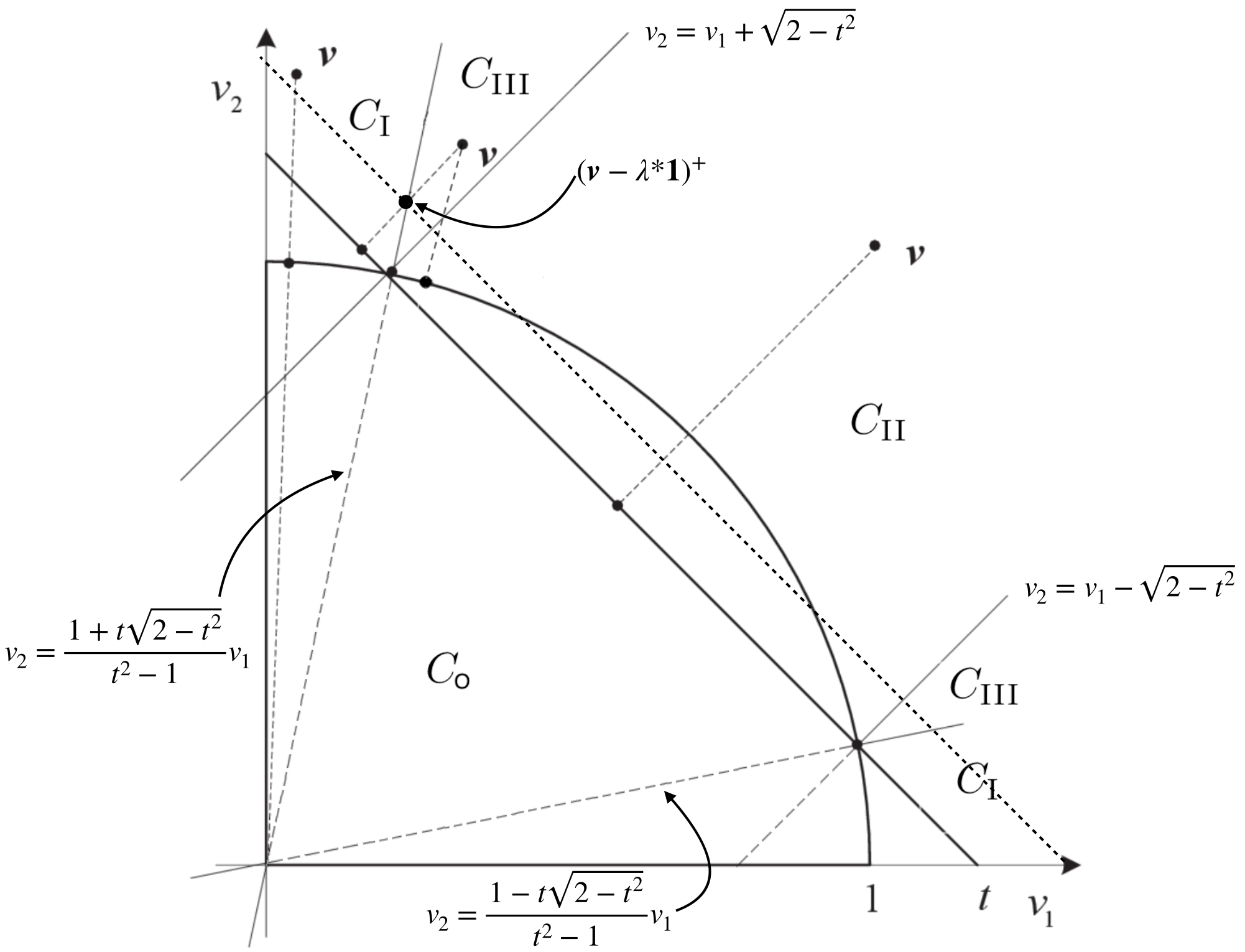
Figure 1: The projection of ${\bm{v}}$ in $\mathbb{R}^{2}$.

4.2 Projection onto $\mathbb{S}_{1}^{t}\cap\mathbb{S}_{2}\cap{\mathbb{R}}^{n}_{+}$

We characterize the projections onto $\mathbb{S}_{1}^{t}\cap\mathbb{S}_{2}\cap{\mathbb{R}}^{n}_{+}$, i.e., the optimal solution of (3.3). By Theorem 4.1, we can consider the Lagrangian dual problem of (3.3),

$$\begin{array}[]{ll}{\rm maximize}&g(\lambda,\mu)\\ {\rm subject\ to}&\mu\geq-1.\end{array} \mathcal{D}_{2}$$ ()

and let $(\lambda^{*},\mu^{*})$ solve the dual ($\mathcal{D}_{2}$). If the solution ${\bm{x}}^{*}$ of ($\mathcal{P}$) for given dual feasible $(\lambda^{*},\mu^{*})$ is primal feasible for (3.3), then $g(\lambda^{*},\mu^{*})=\tfrac{1}{2}\|{\bm{x}}^{*}-{\bm{v}}\|_{2}^{2}$. We get ${\bm{x}}^{*}$ solves (3.3). Therefore, for such ${\bm{x}}^{*}$, we only have to verify its satisfaction of the constraints of (3.3).

Theorem 4.3.

For any ${\bm{v}}\in{\mathbb{R}}^{n}$, one of the following statements must be true:

1. If $I_{1}>t^{2}$, the solution of (3.3) is not unique. Any solution of the system

   $$\sum_{i\in\mathcal{I}_{1}}x_{i}=t,\sum_{i\in\mathcal{I}_{1}}x_{i}^{2}=1,x_{i}\geq 0,i\in\mathcal{I}_{1},x_{i}=0,i\notin\mathcal{I}_{1}$$ (4.8)

   solves (3.3).

2. If $I_{1}=t^{2}$, then (3.3) has the unique solution

   $$x_{i}=1/\sqrt{I_{1}},i\in\mathcal{I}_{1}\ \text{ and }\ x_{i}=0,i\notin\mathcal{I}_{1},$$

   which is also the unique solution of (4.8).

3. If $I_{1}<t^{2}$, then (3.3) has the unique solution ${\bm{x}}=({\bm{v}}-\lambda^{*}\mathbf{1})^{+}/\|({\bm{v}}-\lambda^{*}\mathbf{1})^{+}\|_{2},$ where $\lambda^{*}$ is the unique root of $\phi(\lambda)=0$ on $(-\infty,v_{\max})$.

Proof.

(i) If $I_{1}>t^{2}$, by Proposition 3.4(i), $\phi(\lambda)$ has no root on $(0,v_{\max})$. By Lemma 4.1(ii), $g(\lambda,\mu)$ has no stationary point in the region ${\mathbb{R}}\times(-1,\infty)$. Therefore, the optimal solution of ($\mathcal{D}_{2}$) is $\lambda^{*}=\lambda_{1},\mu^{*}=-1$. By Lemma 4.1(i), any point ${\bm{x}}$ satisfying (4.8) must be a solution of ($\mathcal{P}$), since it satisfies (4.1). Moreover, it satisfies the constraints of (3.3), so that it is optimal. This completes the proof of (i).

(ii) If $I_{1}=t^{2}$, $\phi(\lambda)\equiv 0$ on $[\lambda_{2},v_{\max})$ by Proposition 3.4(ii), we can see that any $(\lambda,\mu)$ with $\lambda\in[\lambda_{2},\lambda_{1})$ and $\mu=\|({\bm{v}}-\lambda{\bm{1}})^{+}\|_{2}-1$ is stationary for the dual ($\mathcal{D}_{2}$). For those $(\lambda,\mu)$, by Lemma 4.1(ii), the solution of ($\mathcal{P}$) satisfies $x_{i}(\lambda,\mu)>0$, $i\in{\mathcal{I}}_{1}$ and $x_{i}(\lambda,\mu)=0$, $i\notin{\mathcal{I}}_{1}$. If we further require the satisfaction of the constraints of (3.3), then there is only a unique point $x_{i}^{*}=\tfrac{1}{\sqrt{I_{1}}}$ for $i\in\mathcal{I}_{1}$ and $x_{i}^{*}=0$ for $i\notin\mathcal{I}_{1}$ since $I_{1}=t^{2}$. This completes the proof of (ii).

(iii) If $I_{1}<t^{2}$, $\phi(\lambda)=0$ has a unique root $\lambda^{*}$ in $(-\infty,v_{\max})$ by Proposition 3.4(iii). Therefore, by (4.4) the optimal solution $(\lambda^{*},\mu^{*})$ of ($\mathcal{D}_{2}$) satisfies $\mu^{*}=\|({\bm{v}}-\lambda^{*}{\bm{1}})^{+}\|_{2}-1$. Given $(\lambda^{*},\mu^{*})$, by (4.2), the solution of ($\mathcal{P}$) is given in (4.7). It can be easily verified that ${\bm{x}}^{*}$ is feasible for (3.3). Therefore, ${\bm{x}}^{*}$ solves (3.3), completing the proof of (iii). ∎

4.3 Projection onto $\mathbb{B}_{1}^{t}\cap\mathbb{S}_{2}\cap{\mathbb{R}}^{n}_{+}$

We consider the Lagrangian dual problem of (3.2)

$$\begin{array}[]{ll}{\rm maximize}&g(\lambda,\mu)\\ {\rm subject\ to}&\lambda\geq 0,\mu\geq-1.\end{array} \mathcal{D}_{3}$$ ()

and let $(\lambda^{*},\mu^{*})$ be optimal for the dual ($\mathcal{D}_{3}$). If the optimal solution ${\bm{x}}^{*}$ of ($\mathcal{P}$) for given dual feasible $(\lambda^{*},\mu^{*})$ is also primal feasible for (3.2) and $(\lambda^{*},\mu^{*})$ and ${\bm{x}}^{*}$ satisfy complementarity

$$\lambda^{*}(\mathbf{1}^{T}{\bm{x}}^{*}-t)=0,$$ (4.9)

then $g(\lambda^{*},\mu^{*})=\tfrac{1}{2}\|{\bm{x}}^{*}-{\bm{v}}\|_{2}^{2}$. So ${\bm{x}}^{*}$ is optimal for (3.2).

We characterize the projections onto $\mathbb{B}_{1}^{t}\cap\mathbb{S}_{2}\cap{\mathbb{R}}^{n}_{+}$ below.

Theorem 4.4.

For any ${\bm{v}}\in{\mathbb{R}}^{n}$, one of the following statements must be true:

1. Suppose $v_{\max}>0$, $I_{1}\leq t^{2}$ and $\|{\bm{v}}^{+}\|_{1}>t\|{\bm{v}}^{+}\|_{2}$. Then (3.2) has a unique solution $({\bm{v}}-\lambda^{*}\mathbf{1})^{+}/\|({\bm{v}}-\lambda^{*}\mathbf{1})\|_{2},$ where $\lambda^{*}$ is the unique root of $\phi(\lambda)=0$ on $(0,v_{\max})$.

2. Suppose $v_{\max}>0$, $I_{1}\leq t^{2}$ and $\|{\bm{v}}^{+}\|_{1}\leq t\|{\bm{v}}^{+}\|_{2}$. Then (3.2) has a unique solution ${\bm{v}}^{+}/\|{\bm{v}}^{+}\|_{2}$.

3. Suppose $v_{\max}>0$ and $I_{1}>t^{2}$. Then the solution of (3.2) is not unique. Any point satisfying (4.8) is the optimal solution of (3.2).

4. Suppose $v_{\max}=0$. The solution of (3.2) is not unique. Any ${\bm{x}}$ satisfying

   $$\sum_{i\in\mathcal{I}_{1}}x_{i}\leq t,\sum_{i\in\mathcal{I}_{1}}x_{i}^{2}=1,x_{i}\geq 0,i\in\mathcal{I}_{1},x_{i}=0,i\notin\mathcal{I}_{1}$$ (4.10)

   is optimal for (3.2).

5. Suppose $v_{\max}<0$. Any ${\bm{x}}$ satisfying $x_{i}=1$ for some $i\in\mathcal{I}_{1}$ and $x_{j}=0$ for $j\neq i$ is optimal for (3.2).

Proof.

(i) If $I_{1}=t^{2}$, by Proposition 3.4(ii), $\phi(\lambda)=0$ for any $\lambda\in[\lambda_{2},v_{\max})$. If $I_{1}>t^{2}$, notice that $\|{\bm{v}}^{+}\|_{1}>t\|{\bm{v}}^{+}\|_{2}$ is equivalent to $\phi(0)>0$; by Proposition 3.4(iii), $\phi(\lambda)=0$ has a unique solution $\lambda^{*}$ on $(0,v_{\max})$. In both cases, we let $\mu^{*}=\|({\bm{v}}-\lambda^{*}{\bf 1})^{+}\|_{2}-1$. Then by Lemma 4.1(ii), we have $\nabla g(\lambda^{*},\mu^{*})=0$. So $(\lambda^{*},\mu^{*})$ is the optimal solution of ($\mathcal{D}_{3}$). In this case, ${\bm{x}}^{*}=({\bm{v}}-\lambda^{*}\mathbf{1})^{+}/\|({\bm{v}}-\lambda^{*}\mathbf{1})\|_{2}$ is the solution of (3.2) and is feasible for (3.2). In addition, $(\lambda^{*},\mu^{*},{\bm{x}}^{*})$ satisfies (4.9). This proves (i).

(ii) Same argument as for (i) implies that $\mu^{*}>-1$. Since $\|{\bm{v}}^{+}\|_{1}\leq t\|{\bm{v}}^{+}\|_{2}$, letting $(\lambda^{*},\mu^{*})$ with $\lambda^{*}=0$ and $\mu^{*}=\|{\bm{v}}^{+}\|_{2}-1$, we have

$$\ \frac{\partial g(\lambda^{*},\mu^{*})}{\partial\lambda}(\lambda-\lambda^{*})+\frac{\partial g(\lambda^{*},\mu^{*})}{\partial\mu}(\mu-\mu^{*})$$ (4.11)

$$= \ (\|{\bm{v}}^{+}\|_{1}/\|{\bm{v}}^{+}\|_{2}-t)\lambda+0(\mu-\mu^{*})$$

$$\leq \ 0$$

for any $\lambda\geq 0,\mu\geq 0$. Therefore, $(\lambda^{*},\mu^{*})$ is the optimal solution of ($\mathcal{D}_{3}$). For given $(\lambda^{*},\mu^{*})$, by (4.2) the solution of ($\mathcal{P}$) is ${\bm{x}}^{*}={\bm{v}}^{+}/\|{\bm{v}}^{+}\|_{2}$. We can see that ${\bm{x}}^{*}$ is feasible for (3.2). $(\lambda^{*},\mu^{*},{\bm{x}}^{*})$ obviously satisfies (4.9). This proves (ii).

(iii) Let $v_{\max}>0$ and $I_{1}>t^{2}$. By Proposition 3.4(i), $\phi(\lambda)=0$ does not have root on $(-\infty,v_{\max})$. By Lemma 4.1(ii), $g(\lambda,\mu)$ has no stationary point in the region ${\mathbb{R}}\times(-1,\infty)$. Therefore, the optimal solution of ($\mathcal{D}_{2}$) is $\lambda^{*}=\lambda_{1},\mu^{*}=-1$. By Lemma 4.1(i), any point ${\bm{x}}$ satisfying (4.8) must be a solution of ($\mathcal{P}$), since it satisfies (4.1). Moreover, it satisfies the constraints of (3.3). In addition, any ${\bm{x}}$ satisfying (4.8) with $\lambda^{*}=0$ and $\mu^{*}=-1$ also satisfies (4.9). This completes the proof of (iii).

(iv) Let ${\bm{v}}^{+}=0$ and $\lambda_{1}=0$. It must be true that $\mu^{*}=-1$ since otherwise $\nabla g(\lambda,\mu)\neq 0$ for any $\lambda\geq 0$ and $\mu>-1$ by (4.3) and (4.4). This indicates by Lemma 4.1(i) that $\lambda^{*}=v_{\max}=0$. For $(\lambda^{*},\mu^{*})=(0,-1)$, by (4.1) the solution of (4.10) solves ($\mathcal{P}$) and those ${\bm{x}}$ are feasible for (3.2). Therefore, any ${\bm{x}}$ satisfying (4.10) must be optimal for (3.2). This proves (iv).

(v) Let ${\bm{v}}^{+}=0$ and $\lambda_{1}<0$. Same argument applied to the proof of (iv) implies that the optimal solution of the dual ($\mathcal{D}_{3}$) is $(\lambda^{*},\mu^{*})=(0,-1)$. However, by (4.1) the solution of ($\mathcal{P}$) is ${\bm{x}}=0$ which is infeasible for (3.2). Therefore, we further investigate the primal optimal solution and rewrite (3.2) as

$$\mathop{\rm minimize}-{\bm{v}}^{T}{\bm{x}}\quad{\rm subject\ to}\ \ {\bm{x}}\in\mathbb{R}^{n}_{+}\cap\mathbb{B}_{1}^{t}\cap\mathbb{S}_{2}.$$ (4.12)

Since $-{\bm{v}}^{T}{\bm{x}}\geq(-\lambda_{1})\bm{1}^{T}{\bm{x}}$ for all ${\bm{x}}\in\mathbb{R}_{+}^{n}$ and equality holds if and only if $x_{i}=0$ for $i\notin\mathcal{I}_{1}$ since $-\lambda_{1}>0$. Hence, we can instead consider minimize $\bm{1}^{T}{\bm{x}}$ and obtain

$$\mathop{\rm minimize}\bm{1}^{T}{\bm{x}}\quad\ \ {\rm subject\ to}\quad{\bm{x}}\in\mathbb{R}^{n}_{+}\cap\mathbb{S}_{2}.$$ (4.13)

Notice the constraint $\sum_{i=1}^{n}x_{i}\leq t$ is eliminated since $\sum_{i=1}^{n}x_{i}$ is minimized in the objective; this constraint must be satisfied at the optimal solution of (4.13) since otherwise (4.12) is infeasible. The optimal solution of (4.13) is obviously any ${\bm{x}}$ with exactly one nonzero component, i.e., $x_{i}=1$ for some $i\in\{1,\ldots,n\}$, and such points are naturally feasible for $\sum_{i=1}^{n}x_{i}\leq t$ due to the assumption $t>1$. On the other hand, if we further require $i\in{\mathcal{I}}_{1}$, then $-{\bm{v}}^{T}{\bm{x}}=-\lambda_{1}\bm{1}^{T}{\bm{x}}$, meaning $-{\bm{v}}^{T}{\bm{x}}$ attains the minimum of $-\lambda_{1}\bm{1}^{T}{\bm{x}}$ on the same feasible region. Therefore, any ${\bm{x}}$ with only one nonzero component $x_{i}=1$ and $i\in{\mathcal{I}}_{1}$ is optimal for (3.2). Case (iv) is also true. ∎

5 Proposed Algorithms for Solving $\phi=0$

Based on Theorems 4.2, 4.3 and 4.4, the projections onto $\mathbb{B}_{1}^{t}\cap\mathbb{B}_{2}$, $\mathbb{S}_{1}^{t}\cap\mathbb{S}_{2}$ and $\mathbb{B}_{1}^{t}\cap\mathbb{S}_{2}$, as well as the problem of maximizing a linear function over the $\mathbb{B}_{1}^{t}\cap\mathbb{B}_{2}$ can all revert to solving the equation of $\phi(\lambda)=0$. If we can design an algorithm to quickly find the root, then all the problems above can be solved efficiently. Instead of presenting algorithms for solving each of the projection problems, in this section, we focus on designing algorithms for computing the root of $\phi(\lambda)=0$. Once we have the root of $\phi(\lambda)=0$, we can easily obtain the optimal solution.

5.1 Breakpoint Search with Sorting

In this subsection, we focus on designing algorithms for solving the nonsmooth equation $\phi(\lambda)=0$ by assuming ${\bm{v}}$ is already sorted in descending order. From Proposition 3.3, we know $\phi$ is piecewisely quadratic with breakpoints $\lambda_{1},...,\lambda_{k}$. Therefore, $\phi$ is quadratic on each interval $[\lambda_{j-1},\lambda_{j}]$, $j=2,\ldots,k$. If we know the index $j^{*}$ with $\phi(v_{j^{*}+1})\geq 0$ and $\phi(v_{j^{*}})<0$, then solving $\phi=0$ on $(a,b)$ reverts to solving a quadratic equation with $\lambda$ on $[v_{j^{*}+1},v_{j^{*}})$, which possesses a close form of the root. This motivates us to find such breakpoints $v_{j^{*}+1}$ and $v_{j^{*}}$, or equivalently, the index $j^{*}$. Once this interval is determined, from (3.8), we know $\phi(\lambda)$ has a root $\lambda^{*}$ on $(v_{j^{*}+1},v_{j^{*}})$:

$$\lambda^{*}=\frac{1}{j^{*}}\left(s-t\sqrt{\tfrac{j^{*}w-s^{2}}{j^{*}-t^{2}}}\right).$$ (5.1)

Notice that the projection is often sparse in the applications of interests. We propose a Forward Searching (FS) method to search for $j^{*}$, which checks the function value at each breakpoint in the order of $v_{1},\ldots,v_{n}$ to determine the first index $j$ satisfying $\phi(v_{j+1})\geq 0$. One may also consider other searching strategies, e.g., backward searching in the order of $v_{n},\ldots,v_{1}$.

The major computational cost besides sorting in this method is spent on the function evaluations of $\phi$, which takes $O(n)$ operations per each evaluation. Therefore, it can further reduce the computational cost by updating the function values in the recursive way in our FS method. A complete statement of this method is provided in Algorithm 1.

Algorithm 1 Forward searching (FS) method for solving $\phi(\lambda)=0$.

1:  Input a vector ${\bm{v}}\in{\mathbb{R}}^{n}$ and $t\in(1,\sqrt{n})$

2:  Sort ${\bm{v}}$ in decending order.

3:  Let $j_{t}=\lceil t^{2}\rceil$ and compute $s=\sum_{i=1}^{j_{t}}v_{i}$, $w=\sum_{i=1}^{j_{t}}v_{i}^{2}$.

4:  for $j=j_{t},...,n-1$ do

5:     $s=s+v_{j+1},w=w+v_{j+1}^{2}$;

6:     if $v_{j+1}<v_{j}$ then

7:        $\phi=\ ((j+1)-t^{2})((j+1)v_{j+1}-2sv_{j+1})v_{j+1}+s^{2}-t^{2}w$;

8:        if $\phi\geq 0$ then

9:           $j^{*}=j$; $s=s-v_{j+1},w=w-v_{j+1}^{2}$;

10:           return  

11:        end if

12:     end if

13:  end for

14:  Output $\lambda^{*}=\frac{1}{j^{*}}\left(s-t\sqrt{\frac{j^{*}w-s^{2}}{\hat{j}-t^{2}}}\right)$.

5.2 Improved Bisection Methods

The FS method should be witnessed complexity of $O(n\log n)$ at best due to the presence of sorting. In this subsection, we design a breakpoint search method without sorting, so that in practice faster speed could be witnessed.

The efficiency of the our iterative root-finding algorithms mainly depends on two factors: the computational cost of the function evaluation, and the total number of iterations. Next we discuss techniques to reduce the computational efforts caused by these two factors.

For efficiently evaluating $\phi$, (3.5) and (3.9) imply that the calculation of $\phi(\lambda)$ and the first-order derivative information depends on the calculation of $I_{\lambda},s_{\lambda}$ and $q_{\lambda}$. Notice that the first-order derivative of $\phi$ at $\lambda$ could be the gradient if $\phi$ is differentiable at $\lambda$ or a subgradient of $\phi$ at $\lambda$ if $\phi$ is nondifferentiable, since $\phi$ is convex on $(-\infty,\lambda_{j_{t}}]$ by Proposition 3.3 (v).

Let the interval that we are working on be $[l,r]$ with $\phi(l)>0$ and $\phi(r)<0$, and $\phi(r)$ and $\phi^{\prime}(r)$ have been computed. The set ${\mathcal{I}}_{r}$ and the respective scales $m_{r},s_{r},q_{r}$ have been recorded. We now show how to evaluate the set ${\mathcal{I}}_{\lambda}$ and $I_{\lambda},s_{\lambda},q_{\lambda}$ for any $\lambda\in[l,r)$. Denote ${\mathcal{U}}_{\lambda}=\{i:\lambda\leq v_{i}\leq r,i=1,\ldots,n\}$. Then we have ${\mathcal{I}}_{\lambda}={\mathcal{I}}_{r}\cup{\mathcal{U}}_{\lambda}$, so that

$$I_{\lambda}=m_{r}+|{\mathcal{U}}_{\lambda}|,\ s_{\lambda}=s_{r}+\sum_{i\in{\mathcal{U}}_{\lambda}}v_{i},\ w_{\lambda}=w_{r}+\sum_{i\in{\mathcal{U}}_{\lambda}}v_{i}^{2},$$ (5.2)

implying that we can simply focus on those elements of ${\bm{v}}$ on $[\lambda,r]$ for evaluation $\phi$ and the first-order derivative of $\phi$. Note that the number of elements in ${\bm{v}}$ in the interval $[\lambda,r]$ decreases as the algorithm proceeds, thus the computational cost needed per iteration decreases as well.

Bounding the Root. While solving an equation, it could be extremely helpful if one can find a relatively accurate estimate of the range (interval) containing the root. This can significantly reduce the number of iterations for many algorithms such as bisection method, secant method or even (nonsmooth) Newton method. It has been shown that $\phi(\lambda)=0$ must have a unique root in $(0,v_{\max})$ if $\phi(0)>0$. The next proposition further narrows down the interval containing $\lambda^{*}$.

Proposition 5.1.

For ${\bm{v}}\in\mathbb{R}^{n}_{+}$, suppose $\|{\bm{v}}\|_{1}>t,\ \|{\bm{v}}\|_{1}>t\|{\bm{v}}\|_{2}\ \text{ and }\ \|({\bm{v}}-\hat{\lambda}\mathbf{1})^{+}\|_{2}>1,$ with $\hat{\lambda}$ being the root of $\psi(\lambda)=0$ on ${\mathbb{R}}$, $\lambda^{*}$ be the root $\phi(\lambda)=0$ on $(0,v_{\max})$, and $\tilde{\lambda}:=(\|{\bm{v}}\|_{1}-t\|{\bm{v}}\|_{2})/n>0$. Then $\phi(\tilde{\lambda})>0$ and $\phi(\hat{\lambda})<0$.

Proof.

First of all, by Theorem 4.2, we have $\phi(\hat{\lambda})<0$ and $\hat{\lambda}\in(0,v_{\max})$.

Since $\phi$ is strictly decreasing on $(0,\lambda^{*}]$ by Proposition 3.3 (iv), we only have to prove that $\tilde{\lambda}<\lambda^{*}$ since $\phi(\lambda^{*})=0$. By the definition of $\psi$ it holds true that

$$\psi(\tilde{\lambda})\geq\sum_{i=1}^{n}(v_{i}-\tilde{\lambda})-t=t(\|{\bm{v}}\|_{2}-1)$$ (5.3)

where the equality comes from the definition of $\tilde{\lambda}$. Moreover, by $\hat{\lambda}>0$ and the definition of $\lambda^{*}$, $\psi$ and $\phi$,

$$\psi(\lambda^{*})=\sqrt{\phi(\lambda^{*})+t^{2}\|({\bm{v}}-\hat{\lambda}\bm{1})^{+}\|_{2}^{2}}-t=t\left(\|({\bm{v}}-\hat{\lambda}\bm{1})^{+}\|_{2}-1\right)<t(\|{\bm{v}}\|_{2}-1),$$

which, combined with (5.3), yields $\psi(\tilde{\lambda})>\psi(\lambda^{*})$. It follows that $\tilde{\lambda}<\lambda^{*}$ since $\psi$ is decreasing on $(0,\hat{\lambda})$ by Proposition 2.1, completing the proof. ∎

Proposition 5.1 can be used to initialize Algorithm 2 and 3. In Algorithm 2 and 3 where ${\bm{v}}$ is not sorted, we can set $l=\tilde{\lambda}\ \text{ and }\ r=\hat{\lambda}$ to further alleviate the computational effort.

Reducing the number of iterations. Suppose we are currently working on two endpoints $l$ and $r$ with $\phi(l)>0$ and $\phi(r)<0$. We first derive a tighter upper bound for the root than $r$. Consider the line passing through points $(l,\phi(l))$ and $(r,\phi(r))$:

$$S(\lambda)=\phi(r)+\frac{\phi(l)-\phi(r)}{l-r}(\lambda-r)\ \text{ with root }\ \lambda_{S}=r-\phi(r)\frac{l-r}{\phi(l)-\phi(r)}.$$

Notice that $S(l)=\phi(l)>0$ and $S(r)=\phi(r)<0$, implying $l<\lambda_{S}<r$. Therefore, if we can show $\phi(\lambda_{S})<0$, then $\lambda_{S}$ is a tighter upper bound for the root than $r$.

If $r\leq\lambda_{j_{t}}$, by Proposition 3.3 (iv), $\phi$ is convex on $(l,r)$. Since $S(l)=\phi(l)$ and $S(r)=\phi(r)$, the line $S(\lambda)$ is above the figure of $\phi$ on $[l,r]$, then it holds that $\phi(\lambda_{S})<S(\lambda_{S})=0$.

If $r>\lambda_{j_{t}}$, consider the line $\bar{S}(\lambda)$ passing through points $(l,\phi(l))$ and $(\lambda_{j_{t}},\phi(\lambda_{j_{t}}))$

$$\bar{S}(\lambda)=\phi(\lambda_{j_{t}})+\frac{\phi(\lambda_{l})-\phi(j_{t})}{l-\lambda_{j_{t}}}(\lambda-\lambda_{j_{t}})$$

and denote the root of this line as $\bar{\lambda}$. Notice that $\phi(\lambda_{j_{t}})<0$ by the definition of $j_{t}$. Following the same argument for $S(\lambda)$, it holds that $\phi(\bar{\lambda})<0$. On the other hand, $l-r<l-\lambda_{j_{t}}$ and $\phi(l)-\phi(r)<\phi(l)-\phi(\lambda_{j_{t}})$ since $\phi$ is monotonically increasing on $[\lambda_{j_{t}},v_{\max})$ by Proposition 3.3 (iv). Therefore, $\bar{S}^{\prime}(\lambda)<S^{\prime}(\lambda)<0$, combined with $S(l)=\bar{S}(l)>0$, implying $\lambda_{S}>\bar{\lambda}$. Hence, $\phi(\lambda_{S})<0$ by Proposition 3.3 (iv).

Next, we derive a tighter lower bound for the root than $l$. Consider the line passing through $(l,\phi(l))$ with derivative $\varphi^{\prime}_{j}(l)$, which by Proposition 3.3 (v) can be written as

$$T(\lambda)=\phi(l)+\phi^{\prime}(l)(\lambda-l).$$

Based on the definition of $\varphi^{\prime}_{j}$ in (3.9) and $j\geq j_{t}$ by $\phi(l)>0$, we have $\phi^{\prime}(l)=\varphi^{\prime}_{j}(l)<0$. Therefore the unique root of $T$ is

$$\lambda_{T}=l-\phi(l)/\phi^{\prime}(l)>l.$$ (5.4)

We only have to show that $\phi(\lambda_{T})>0$. To see this, notice that $\phi$ is convex on $(-\infty,\lambda_{j_{t}})$ and $\varphi^{\prime}_{j}(l)\in\partial\phi(l)$ by Proposition 3.3 (v), the line $T(\lambda)$ always underestimate $\phi$, implying $\phi(\lambda_{T})>T(\lambda_{T})=0$.

We finally consider $\phi(\cdot)$ on the interval $(\lambda_{j+1},\lambda_{j})$ containing $l$. It follows that on this interval $\phi$ is equal to the quadratic function

$$\varphi_{j}(\lambda)=(m_{l}-t^{2})m_{l}\lambda^{2}-2(m_{l}-t^{2})s_{l}\lambda+s_{l}^{2}-t^{2}w_{l}.$$

Here $j\geq j_{t}$ since $\phi(l)>0$. Denote the smaller root of $\varphi_{j}$ as $\lambda_{Q}$, then by (3.8),

$$\lambda_{Q}=\frac{1}{m_{l}}\left(s_{l}-t\sqrt{\frac{m_{l}w_{l}-s_{l}^{2}}{m_{l}-t^{2}}}\right),$$ (5.5)

which is shown $\phi(\lambda_{Q})\geq 0$ in the following lemma.

Proposition 5.2.

If no $v_{i}\in(l,\lambda_{Q})$, then $\phi(\lambda_{Q})=0$; otherwise $\phi(\lambda_{Q})>0$.

Proof.

If there no $v_{i}\in(l,\lambda_{Q})$, then $\lambda_{Q}\in(\lambda_{j+1},\lambda_{j})$. So $\phi(\lambda_{Q})=\varphi_{j}(\lambda_{Q})=0$. Otherwise, Since $j\geq j_{t}$, so by Proposition 3.3 (v), it holds that $\phi(\lambda_{Q})>\varphi_{j}(\lambda_{Q})=0$. ∎

Based on the discussion above, we design two methods. One is named as the Semi-Smooth Newton Secant Bisection method (SSNSB). The other is Quadratic Approximation Secant Bisection method (QASB). They are stated in Algorithm 2 and 3 respectivly.

Algorithm 2 Semi-Smooth Newton Secant Bisection (SSNSB) Method for $\phi(\lambda)=0$.

1:  Input a vector ${\bm{v}}\in{\mathbb{R}}^{n}$ and $t\in(1,\sqrt{n})$ and tolerance $\delta$.

2:  Given $r$ and $l$ satisfying $\phi(l)>0$ and $\phi(r)<0$.

3:  while  $r-l>\delta$ and $|\phi(\lambda)|>\delta$ do

4:     Compute $\lambda_{S}$, $\phi(\lambda_{S})$, $\lambda_{T}$, $\phi(\lambda_{T})$, $\lambda=(\lambda_{S}+\lambda_{T})/2$, $\phi(\lambda)$.

5:     if $\phi(\lambda)>0$ then

6:        $r=\lambda_{S}$, $l=\lambda_{T}$.

7:     else

8:        $l=\lambda$, $r=\lambda_{T}$.

9:     end if

10:  end while

11:  Output $\lambda$.

Algorithm 3 Quadratic Approximation Secant Bisection (QASB) Method for $\phi(\lambda)=0$.

1:  Input a vector ${\bm{v}}\in{\mathbb{R}}^{n}$ and $t\in(1,\sqrt{n})$ and tolerance $\delta$.

2:  Given $r$ and $l$ satisfying $\phi(l)>0$ and $\phi(r)<0$.

3:  while  $r-l>\delta$ and $|\phi(\lambda)|>\delta$ do

4:     Compute $\lambda_{S}$, $\phi(\lambda_{S})$, $\lambda_{Q}$, $\phi(\lambda_{Q})$, $\lambda=(\lambda_{S}+\lambda_{Q})/2$, $\phi(\lambda)$.

5:     if there is no $v_{i}$ in $(l,\lambda_{Q})$ then

6:        $\lambda=\lambda_{Q}$.

7:        return  

8:     end if

9:     if $\phi(\lambda)>0$ then

10:        $r=\lambda_{S}$, $l=\lambda_{Q}$.

11:     else

12:        $l=\lambda$, $r=\lambda_{Q}$.

13:     end if

14:  end while

15:  Output $\lambda$.

6 Numerical experiments

In this section, we test the performance of our proposed methods. The experiments consist of two parts. The first part is testing SSNSB and QASB with contemporary methods for computing the projection of a given ${\bm{v}}$ onto ${\mathbb{B}}_{1}^{\text{t}}\cap{\mathbb{B}}_{2}$. The main computational efforts focus on solving $\phi(\lambda)=0$, corresponding to the case where ${\bm{v}}$ lies in region $C_{\text{III}}$ in Table 1 (the hard case). The second part is to test SSNSB and QASB on solving $\phi(\lambda)=0$ for computing the projection onto $\mathbb{S}_{1}^{\text{t}}\cap\mathbb{S}_{2}$.

In all experiments, the tolerance is set as $\delta=10^{-9}$. The codes are implemented in C code, and runs on an HP laptop with a 1.80GHz Intel Core, i7-8565U CPU and 16.0GB RAM for Windows 10. In the table of results, each number is the average of 100 runs with fastest being the numbers in bold and the standard deviation in the parenthesis.

6.1 Projection onto ${\mathbb{B}}_{1}^{\text{t}}\cap{\mathbb{B}}_{2}$

For fixed dimension $n$, we randomly generate the input vector $\bm{v}\in{\mathbb{R}}^{n}$, and keep those that fall in $C_{\text{III}}$ and discard those that are not in $C_{\text{III}}$. We only compare the efficiency of FS, BM (the traditional Bisection method), SSNSB and QASB. Let $\sigma=(\sqrt{n}-t)/(\sqrt{n}-1)$, where $\sigma$ measures sparseness as suggested by Hoyer [6]. We set $\sigma$ for 0.9 as used by [8], and setting $t$ according to the values of $\sigma$ and $n$. We consider the following three types of approaches to generate the data, which is motivated in the test of [17] and represent the components in ${\bm{v}}$ have different mean values.

• Type I: $v_{1},\cdots,v_{n}$ are i.i.d random Guassian numbers with mean $0$ and standard deviation 1.

• Type II: 7/8 components of $\bm{v}$ are i.i.d random Guassian numbers of mean $0$ and standard deviation $0.2$, the rest are i.i.d random Guassian numbers of mean $0.9$ and standard deviation $0.2$.

• Type III: Components of $\bm{v}$ are randomly equally partitioned with i.i.d random Guassian numbers of mean $0.1$, $0.4$, $0.7$, $1.0$ respectively and standard deviation $0.2$.

The initial interval for SSNSB and QASB are chosen as ($\tilde{\lambda}$, $\hat{\lambda}$). As for BM, we test initial interval with ($0$, $v_{\max}$)and ($\tilde{\lambda}$, $\hat{\lambda}$) to show the benefits brought by our proposed initial interval.

An Illustrative Example We generate $\bm{v}$ of Type I with $n=100$ to illustrate the behavior of QASB. Table 2 shows the iteration information of BM, SSNSB and QASB over $k$. We also record $|{\mathcal{U}}|$ of those algorithms during the iteration in Table 3, where Iter. denotes the total number of iterations.

From Table 3, we can see that QASB converges faster than others. Once $\left|{\mathcal{U}}^{k}\right|=0$, QASB terminates, while other methods still need many iterations to terminate. Overall, SSNSB and QASB outperform BM in number of iterations. We can also see that our proposed initial interval is significantly narrowed.

Table 2: The iteration information of QASB terminating in 3 iterations.

$k$	$|{\mathcal{U}}^{k}|$	$l^{k}$	$\lambda_{Q}^{k}$	$\lambda^{k+1}$	$\lambda_{S}^{k}$	$r^{k}$
0	50	0	0.5747	1.4858	1.9600	1.9610
1	6	1.4858	1.8180	1.8846	1.9512	1.9600
2	1	1.8846	1.9271	1.9300	1.9329	1.9512
3	0	1.9271	-	1.9292	-	1.9300

Table 3: $|{\mathcal{U}}|$ of three algorithms on an example of Type I with $n=100$. We use our proposed initial interval $[\tilde{\lambda},\hat{\lambda}]$ for BM, SSNSB and QASB. We also test BM using this interval versus using $[0,v_{\max}]$.

$k$	BM $[0,v_{\max}]$	BM $[\tilde{\lambda},\hat{\lambda}]$	SSNSB	QASB
0	100	50	50	50
1	15	10	8	6
2	12	6	1	1
3	7	2	0	0
4	5	2	0
5	5	1	0
6	1	0	0
7	0	0
$\vdots$	$\vdots$	$\vdots$
31	0	0
32	0
Iter.	32	31	6	3

Number of Iterations We also test the total number of iterations needed by each algorithm for ${\bm{v}}$ with increasing dimension $n=10^{3},10^{5},10^{7}$. The initial interval for all algorithms are set as $[\tilde{\lambda},\hat{\lambda}]$. The results are summarized in Table 4.

Table 4: Iteration steps for solving zero point of $\phi$.

	Type I			Type II			Type III
$n$	BM	SSNSB	QASB	BM	SSNSB	QASB	BM	SSNSB	QASB
$10^{3}$	31.0	6.1	4.0	30.0	6.4	3.8	30.0	6.6	4.0
$10^{5}$	32.0	6.9	4.6	30.0	6.2	5.4	30.0	3.6	5.3
$10^{7}$	32.0	7.0	6.0	31.0	6.4	6.5	30.0	6.3	6.1

We can see from Table 4 that for three types of data, the total number of iterations needed by SSNSB and QASB are all significantly less than BM, and QASB needs usually two or three steps less than SSNSB. Another aspect to notice is that the numbers of iterations needed by SSNSB and QASB remain stable for different sizes of problems.

Computation Efficiency The CPU time (s) for each method is shown in Table 5, where we only record computational time for $\phi=0$ and $N_{z}$ denotes the number of non-zero elements of the obtained solution.

Table 5: Computation time for for solving zero point of $\phi$.

	$n$	$10^{3}$	$10^{5}$	$10^{7}$
	$N_{z}$	3.0e+1	1.9e+3	1.8e+5
Type I	FS	1.7e$-$4(8e$-$6)	1.4e$-$2(2e$-$3)	1.7e$+$0(2e$-$1)
	BM	6.2e$-$5(4e$-$6)	3.6e$-$3(6e$-$4)	3.9e$-$1(4e$-$2)
	SSNSB	2.9e$-$5(1e$-$6)	1.3e$-$3(3e$-$4)	1.9e$-$1(2e$-$2)
	QASB	2.8e$-$5(1e$-$6)	1.3e$-$3(2e$-$4)	1.9e$-$1(2e$-$2)
Type II	FS	1.8e$-$4(2e$-$5)	1.7e$-$2(4e$-$3)	1.6e$+$0(1e$-$1)
	BM	6.7e$-$5(1e$-$5)	4.0e$-$3(1e$-$3)	3.8e$-$1(2e$-$2)
	SSNSB	3.0e$-$5(4e$-$6)	1.5e$-$3(4e$-$4)	1.5e$-$1(1e$-$2)
	QASB	2.7e$-$5(4e$-$6)	1.5e$-$3(4e$-$4)	1.4e$-$1(1e$-$2)
Type III	FS	1.2e$-$4(4e$-$5)	1.5e$-$2(3e$-$3)	1.6e$+$0(6e$-$2)
	SSNSB	2.2e$-$5(8e$-$6)	1.4e$-$3(3e$-$4)	1.6e$-$1(2e$-$2)
	QASB	2.1e$-$5(9e$-$6)	1.4e$-$3(2e$-$4)	1.3e$-$1(2e$-$2)

Table 5 indicates that FS always takes the longest computational time, which is mainly due the sorting procedure in this method. Therefore, it cannot achieved faster observed complexity than $O(n\log n)$. In particular, for large-scale cases ($n=10^{7}$), QASB is substantially outperforms FS and BM. Compared with SSNSB, QASB has obvious advantage in the number of iterations, yet the computational time may not be always superior. The reason behind this observation may be the computational cost per iteration needed by SSNSB is low (simply the evaluation of a univariate quadratic function) when $|{\mathcal{U}}_{\lambda}|=0$.

6.2 Projection onto $\mathbb{S}_{1}^{\text{t}}\cap\mathbb{S}_{2}$

We also apply our methods on computing the projection of ${\bm{v}}$ onto $\mathbb{S}_{1}^{\text{t}}\cap\mathbb{S}_{2}$. In particular, we only consider the situation $\|\bm{v}\|_{1}>t\|\bm{v}\|_{2}$ for a given $t$, in which case the computational effort is spent on solving $\phi(\lambda)=0$ on $(0,|v|_{\text{m}ax})$. We compare QASB with existing algorithms under the situation with initial interval $(0,|v|_{\text{m}ax})$ in the experiment, since it is the fastest method from our previous experiments.

The contemporary algorithms we compare with include:

• Alternating Projection method (AP)[6].

• Newton method (NM1)[8]: NM1 uses Newton method to iterate to find the zero point of $\phi_{1}(\lambda)$. (If the Newton step yields an iterate outside of $[l,r]$, then it proceeds with a bisection iterate $\frac{l+r}{2}$.)

• Newton method (NM2)[8]: it solves $\phi_{2}(\lambda)=0$, a similar method to NM1.

• Forward Search method, (FS)[15]: A forward search method for solving $\phi_{1}(\lambda)=0$ with a sorting procedure.

We use the same data types as used in § 6.1 and compare the CPU time of these four algorithms in Table 6 for $n=10^{3},10^{5},10^{7}$.

Table 6: Comparison of computation times. Each result is the average of 100 realizations with the standard deviations in the parenthesis.

		$n=10^{3}$	$n=10^{5}$	$n=10^{7}$
Type I	FS	7.4e$-$5(3e$-$5)	1.2e$-$2(4e$-$4)	5.2e$+$1(5e$+$0)
	AP	5.7e$-$5(3e$-$5)	6.0e$-$3(3e$-$4)	1.5e+0(6e$-$1)
	NM1	1.5e$-$5(4e$-$5)	1.0e$-$3(1e$-$4)	2.6e$-$1(6e$-$2)
	NM2	2.0e$-$5(4e$-$5)	1.5e$-$3(1e$-$4)	3.4e$-$1(4e$-$2)
	QASB	1.8e$-$5(4e$-$5)	1.8e$-$3(1e$-$4)	3.5e$-$1(9e$-$2)
Type II	FS	1.7e$-$4(2e$-$5)	1.9e$-$2(3e$-$3)	4.5e$+$1(2e+0)
	AP	1.2e$-$4(2e$-$5)	8.5e$-$3(1e$-$3)	1.2e$+$0(3e$-$1)
	NM1	3.5e$-$5(6e$-$6)	1.8e$-$3(2e$-$4)	2.6e$-$1(4e$-$2)
	NM2	4.3e$-$5(7e$-$6)	2.3e$-$3(4e$-$4)	3.1e$-$1(4e$-$2)
	QASB	3.5e$-$5(5e$-$6)	1.7e$-$3(3e$-$4)	2.3e$-$1(1e$-$2)
Type III	FS	7.2e$-$5(2e$-$5)	1.2e$-$2(4e$-$3)	3.0e$+$1(1e$+$0)
	AP	6.0e$-$5(2e$-$5)	6.1e$-$3(2e$-$3)	8.5e$-$1(1e$-$1)
	NM1	1.8e$-$5(6e$-$6)	1.3e$-$3(5e$-$4)	1.8e$-$1(2e$-$2)
	NM2	1.8e$-$5(5e$-$6)	1.3e$-$3(5e$-$4)	1.8e$-$1(2e$-$2)
	QASB	1.8e$-$5(4e$-$6)	1.1e$-$3(5e$-$4)	1.3e$-$1(5e$-$3)

From Table 6, we can see that NM1 is the fastest for Type I data, and QASB is the fastest for Type II and Type III data.

7 Conclusions

In this paper, we have proposed, analyzed, and tested a unified approach for computing the projections onto the intersections of $\ell_{1}$ and $\ell_{2}$ balls or spheres. Novelties of our work is the proposed auxiliary function along with its properties for characterizing the optimal solutions and a unified approach for computing the solutions. The proposed approach has bisection and Newton method implementations that can work with/without sorting. The worst-case complexity of the proposed methods without sorting are $O(n\log n)$ and the complexity in practice is observed to be $O(n)$. Our numerical experiments have demonstrated the efficiency of the proposed methods.

Acknowledgements This research was supported by National Natural Science Foundation of China under Grant 11822103.

References

• [1] Jolliffe, I.T., Trendafilov, N.T., Uddin, M.: A modified principal component technique based on the lasso. Journal of computational and Graphical Statistics 12(3), 531–547 (2003)
• [2] Luss, R., Teboulle, M.: Convex approximations to sparse pca via lagrangian duality. Operations Research Letters 39(1), 57–61 (2011)
• [3] Sigg, C., Buhmann, J.: Expectation-maximization for sparse and non-negative pca. In: Machine Learning, Proceedings of the Twenty-Fifth International Conference (ICML 2008), pp. 960–967 (2008). DOI 10.1145/1390156.1390277
• [4] Witten, D.M., Tibshirani, R., Hastie, T.: A penalized matrix decomposition, with applications to sparse principal components and canonical correlation analysis. Biostatistics 10(3), 515–534 (2009)
• [5] Tenenhaus, A., Philippe, C., Guillemot, V., Le Cao, K.A.K.A., Grill, J., Frouin, V.: Variable Selection for Generalized Canonical Correlation Analysis. Biostatistics 15(3), 569–583 (2014). URL https://hal-supelec.archives-ouvertes.fr/hal-01071432
• [6] O. Hoyer, P.: Non-negative matrix factorization with sparseness constraints. Journal of Machine Learning Research 5, 1457–1469 (2004)
• [7] Potluru, V.K., Plis, S.M., Roux, J.L., Pearlmutter, B.A., Calhoun, V.D., Hayes, T.P.: Block coordinate descent for sparse nmf. arXiv preprint arXiv:1301.3527 (2013)
• [8] Thom, M., Rapp, M., Palm, G.: Efficient dictionary learning with sparseness-enforcing projections. International Journal of Computer Vision 114(2-3), 168–194 (2015)
• [9] Duchi, J., Shalev-Shwartz, S., Singer, Y., Chandra, T.: Efficient projections onto the $\ell_{1}$-ball for learning in high dimensions. Proceedings of the 25th International Conference on Machine Learning pp. 272–279 (2008). DOI 10.1145/1390156.1390191
• [10] Liu, J., Ye, J.: Efficient euclidean projections in linear time. In: Proceedings of the 26th Annual International Conference on Machine Learning, pp. 657–664. ACM (2009)
• [11] Songsiri, J.: Projection onto an $\ell_{1}$-norm ball with application to identification of sparse autoregressive models. In: Asean Symposium on Automatic Control (ASAC) (2011)
• [12] Condat, L.: Fast projection onto the simplex and the $\ell_{1}$ ball. Mathematical Programming 158(1-2), 575–585 (2016)
• [13] Wei Yu, A., Su, H., Li, F.F.: Efficient euclidean projections onto the intersection of norm balls. In: Proceedings of the 29th International Conference on Machine Learning, ICML 2012, vol. 1 (2012)
• [14] Theis, F.J., Stadlthanner, K., Tanaka, T.: First results on uniqueness of sparse non-negative matrix factorization. In: In Proceedings of the 13th European Signal Processing Conference (EUSIPCO05) (2005)
• [15] Gloaguen, A., Guillemot, V., Tenenhaus, A.: An efficient algorithm to satisfy $\ell_{1}$ and $\ell_{2}$ constraints. In: 49èmes Journées de Statistique. Avignon, France (2017). URL https://hal.archives-ouvertes.fr/hal-01630744
• [16] Gong, P., Gai, K., Zhang, C.: Efficient euclidean projections via piecewise root finding and its application in gradient projection. Neurocomputing 74(17), 2754–2766 (2011)
• [17] Dimitris Bertsimas, A.K., Mazumder, R.: Best subset selection via a modern optimization lens. The Annals of Statistics 44, 813–852 (2016). DOI 10.1214/15-AOS1388