Dark photon manifestation in the tripletlike QED processes $\gamma+\ell_{i}\to\ell^{+}_{j}\ell^{-}_{j}+\ell_{i}$, $i\neq j,$ $i=e,\mu,$ $j=e,\mu,\tau$

Abstract

The tripletlike QED processes $\gamma+\ell_{i}\to\ell^{+}_{j}\ell^{-}_{j}+\ell_{i}$ with $i\neq j$, and $i=e,\mu,$ $j=e,\mu,\tau$ has been investigated as the reactions where a dark photon, $A^{\prime}$, is produced as a virtual state with subsequent decay into a $\ell^{+}_{j}\ell^{-}_{j}$ pair. This effect arises due to the so-called kinetic mixing and is characterized by a small parameter $\epsilon$ describing the coupling strength relative to the electric charge $e$. In these processes, the dark photon appears as a resonance with Breit-Wigner propagator in the $\ell^{+}_{j}\ell^{-}_{j}$ system. The distributions over the invariant mass of the produced $\ell^{+}_{j}\ell^{-}_{j}$ pair is calculated and the value of the parameter $\epsilon$, as a function of the dark photon mass, is estimated for a given number of measured events in the specific experimental conditions. Assuming a standard deviation of $\sigma=2$ (corresponding to $\approx$ 95 $\%$ confidence limit) and a number of measured events equal to $10^{4}$, we obtain the following limits for the parameter space of the dark photon: $\epsilon^{2}\leq 10^{-7}$ ($\gamma+\mu^{-}\to e^{+}+e^{-}+\mu^{-}$) and $\epsilon^{2}\leq 10^{-7}\div 6\times 10^{-8}$ ($\gamma+e^{-}\to\mu^{+}+\mu^{-}+e^{-}$) in the $A^{\prime}$ mass region 520 $<m_{A^{\prime}}<$980 MeV. In the mass region 30 $<M_{A^{\prime}}<$400 MeV we obtain $\epsilon^{2}\leq 10^{-7}$ ($\gamma+\mu^{-}\to e^{+}+e^{-}+\mu^{-}$).

I Introduction

Cosmological and astrophysical measurements give evidence of the existence of dark matter. Its nature and interaction are unknown today. The recent experimental discoveries, such as neutrino oscillations (that imply massive neutrinos Fukuda et al. (1998)), and the discrepancy between the Standard Model (SM) prediction and the measured value of the anomalous magnetic moment of the muon Jegerlehner and Nyffeler (2009), as well as recent measurements of flavor-changing processes in B meson decays (showing tensions with the SM predictions Wackeroth (2019)), lead one to consider physics beyond the SM (see the reviews Hewett et al. (2012); Essig, R. and Jaros, J.A. and Wester, W. (2013); Soffer (2015); Alexander et al. (2016)). The extension of the SM includes various models predicting a number of new particles. The so-called dark photon (DP), $A^{\prime}$, is one of the possible new particles. It is a massive vector boson that can mix with the ordinary photon via ”kinetic mixing” Holdom (1986). Its mass and interaction strength are not predicted unambiguously by the theory, since DPs can arise via different mechanisms. Various theoretically motivated regions of the DP mass are given in Ref. Hewett et al. (2012). A DP with mass larger than 1 MeV can be produced in electron (proton) fixed-target experiments or at hadron or electron-positron colliders (see the references in the review Hewett et al. (2012)). The properties of a DP with a mass in the range eV - keV can be determined using astrophysical data.

A number of experiments searching for DPs are carried out or planned in various laboratories. Using APEX test run data obtained at the Jefferson Laboratory Essig et al. (2011); Abrahamyan et al. (2011), the DP was searched in electron-nucleus fixed-target scattering in the mass range 175$\div$250 MeV. The DarkLight Collaboration Freytsis et al. (2010) (JLab) studied the prospects for detecting a light boson with mass $m_{X}\leq$ 100 MeV in electron-proton scattering. The produced $A^{\prime}$ decays to an $e^{+}e^{-}$ pair leading to the $e^{-}pe^{+}e^{-}$ final state. An exclusion limit for the electromagnetic production of a light A^′ decaying to $e^{+}e^{-}$ was determined by the A1 Collaboration at the Mainz Microtron MAMI ( Merkel et al. (2011) using electron scattering from a heavy nucleus. The Heavy Photon Search (HPS) experiment Bravo (2019) searches for an electroproduced DP using an electron beam provided by the Continuous Electron Beam Accelerator Facility accelerator at JLab. HPS looks for DPs through two distinct methods - the search of a resonance in the $e^{+}e^{-}$ invariant mass distribution above the large QED background (large DP-SM particles coupling region) - and the search of a displaced vertex for long-lived DPs (small coupling region).

The manifestation of DPs is also searched for in the decay of known particles. The authors of Ref. Frlez et al. (2004) have studied the radiative pion decay, $\pi^{+}\rightarrow e^{+}\nu\gamma$. The measurements were performed at the $\pi$E1 channel of the Paul Scherrer Institute, Switzerland. The DP was also searched for in the decay of $\pi^{0}$-mesons ($\pi^{0}\rightarrow\gamma A^{\prime}\rightarrow\gamma e^{+}e^{-}$) produced in proton-nuclei collisions at the Heavy Ion Accelerator Facility (China) Wang et al. (2013). The decay of $\pi^{0}$-meson was the tool to search for the DP also in the experiment at WASA-at-COSY(Jülich, Germany) ($\pi^{0}$-mesons were produced in the reaction $pp\rightarrow pp\pi^{0}$) Moskal et al. (2014) and at CERN, where $\pi^{0}$-mesons were produced in the decay of $K$-mesons, $K^{\pm}\rightarrow\pi^{\pm}\pi^{0}$ Goudzovski (2015).

The search for a DP signal in inclusive dielectron spectra in proton-induced reactions on either a liquid hydrogen target or on a nuclear target was performed at the GSI in Darmstadt Agakishiev et al. (2014). An upper limit on the DP mixing parameter in the mass range $m(A^{\prime})=0.02-0.6$ GeV/$c^{2}$ was established. The constraints on the DP parameters from the data collected in experiments with electron beams were summarized in Ref. Andreas (2012). At JLab, it was demonstrated that electron-beam fixed-target experiments would have a powerful discovery potential for DPs in the MeV-GeV mass range Izaguirre et al. (2014). Reference Inguglia (2019) describes some of the main dark sector searches performed by the Belle II experiment at the SuperKEKB energy-asymmetric $e^{+}e^{-}$ collider (a substantial upgrade of the B factory facility at the Japanese KEK laboratory). The design luminosity of the machine is $8\times 10^{35}$ cm^-2s^-1. At Belle II, the DP is searched for in the reaction $e^{+}e^{-}\to\gamma_{ISR}A^{\prime}$, with subsequent decays of the DP to dark matter $A^{\prime}\to\chi\bar{\chi}$ (ISR stays for initial state radiation). The main backgrounds come from QED processes such as $e^{+}e^{-}\to e^{+}e^{-}\gamma(\gamma)$ and $e^{+}e^{-}\to\gamma\gamma(\gamma)$. Preliminary studies have been performed and the sensitivity to the kinetic mixing parameter strength is given. With a small integrated luminosity a very competitive measurement is possible, especially in the region for $M_{A^{\prime}}>$ few times $10$ MeV/$c^{2}$ where the BABAR experiment starts dominating in terms of sensitivity Lees et al. (2017). An experiment to search for $A^{\prime}$ was proposed at VEPP-3 (electron-positron collider) (Russia) Wojtsekhowski (2009). The search method is based on the missing mass spectrum in the reaction $e^{+}e^{-}\to\gamma A^{\prime}$. At the future CEPC experiment (China) running at $\sqrt{s}=91.2$ GeV it is possible for CEPC to perform a decisive measurement on a DP in the mass region 20 GeV $<m_{A^{\prime}}<$ 60 GeV, in about 3 months of operation Jiang et al. (2019). $\sqrt{s}=$ 240 GeV is also achievable.

DP formation in various reactions was investigated theoretically in a number of papers. Bjorken et al. Bjorken et al. (2009) considered several possible experimental setups for experiments aimed at the search for $A^{\prime}$ in the most probable range of masses from a few MeV to several GeV and confirmed that the experiments at a fixed target perfectly suit for the discovery of DPs in this interval of masses. DP production in the process of electron scattering on a proton or on heavy nuclei has been investigated in Ref. Beranek et al. (2013) (Ref. Beranek and Vanderhaeghen (2014)) for the experimental conditions of the MAMI (JLab) experiment Merkel et al. (2011) (Ref. Abrahamyan et al. (2011)). The authors of Ref. Chiang and Tseng (2017) proposed to use rare leptonic decays of kaons and pions $K^{+}(\pi^{+})\rightarrow\mu^{+}\nu_{\mu}e^{+}e^{-}$ to study the light DP (with a mass of about 10 MeV). The constraints on DPs in the 0.01-100 keV mass range are derived in Ref. An et al. (2015) (the indirect constraints following from $A^{\prime}\rightarrow 3\gamma$ decay are also revisited). The proposal to search for light DPs using the Compton-like process, $\gamma e\rightarrow A^{\prime}e$, in a nuclear reactor was suggested in Ref. Park (2017). This suggestion was developed in Ref. Ge and Shoemaker (2018), where the constraints on some DP parameters were determined using the experimental data obtained at the Taiwan EXperiment On NeutrinO reactor (TEXONO). Some results on the phenomenology of the DP in the mass range of a few MeV to GeV have been presented in Ref. Pospelov (2009), where $g$ - 2 of muons and electrons together with other precision QED data, as well as radiative decays of strange particles were analyzed.

The process of the triplet photoproduction on a free electron, $\gamma+e^{-}\to e^{+}+e^{-}+e^{-}$, in which $A^{\prime}$ can be formed as an intermediate state with subsequent decay into an $e^{+}e^{-}$ pair was investigated in Ref. Gakh et al. (2018). The advantage of this process is that the background is a purely QED process $\gamma+e^{-}\to e^{+}+e^{-}+e^{-}$, which can be calculated with the required accuracy. The analysis was done by taking into account the identity of the final electrons. The constraints on parameter $\epsilon$ depending on the DP mass and the statistics (number) of events were obtained with a special method of gathering events where the invariant mass of one $e^{+}e^{-}$ pair remains fixed while the other pair is scanned.

The search for DPs produced at $e^{+}e^{-}$ colliders in the forward region was considered in Ref. Chen et al. (2020). An additional detector set around BESIII can probe the DP coupling parameter $\epsilon$ down to $2\times 10^{-4}$, whereas at Belle-II, it would have a higher sensitivity down to $2\times 10^{-5}$.

It should be mentioned that the constraints on the DP parameters can be obtained using astrophysical data and that the astrophysical constraints on the DP with masses in the range $M_{A^{\prime}}\leq$ (eV-keV) are stronger than laboratory constraints (see, for example, Refs. Jaeckel and Ringwald (2010); Raffelt (1996)). The calculation of the cooling rates for the Sun gives the following constraint on the DP parameter space ($m_{A^{\prime}}<0.1$ eV) An et al. (2013):

$$\epsilon\times\frac{m_{A^{\prime}}}{eV}<1.4\times 10^{-11}.$$

The magnetometer data from $Voyager$ Pignol et al. (2015) probes DPs in the $10^{-24}$ to $10^{-19}$ eV mass range. Values of the coupling parameter $\epsilon$ as low as $3\times 10^{-5}$ for the highest masses were excluded. The proposed search for DPs using the Alpha Magnetic Spectrometer Feng et al. (2016) has a potential discovery for mass $m_{A^{\prime}}\sim{\cal{O}}$(100) MeV and kinetic mixing parameters $10^{-10}\leq\epsilon\leq 10^{-8}$. More information about DP (and dark matter) searches in astrophysical experiments can be found in Ref. Battaglieri et al. (2017).

In this work, we suggest a possible way to detect the DP signal through the reaction $\gamma+\ell_{i}\to\ell^{+}_{j}\,\ell^{-}_{j}+\ell_{i}$ ($\ell$ is a lepton), where a few tens MeV photon collides with a high-energy electron or muon beam. The advantage of this reaction, as compared with the reaction $\gamma+e^{-}\to e^{+}+e^{-}+e^{-}$ considered in Ref. Gakh et al. (2018), is that there are no identical particles in the final state. So, the analysis of the experimental results is simpler. We calculate the distributions over the invariant mass of the produced $\ell^{+}_{j}\ell^{-}_{j}$- pair and search for the kinematical region where the Compton-type diagram contribution is not suppressed with respect to the Borsellino ones. The distributions for the proposed reaction are more interesting (corresponding to a larger number of events) due to the increased phase space, since it is not necessary to fix the parameters of the second pair. We estimated the value of the parameter $\epsilon$ as a function of the DP mass, for a given number of measured events.

This work is organized in the following way: Section II contains the formalism for calculating the distribution over the invariant mass of the produced lepton pair. The kinematics of the proposed reaction is briefly considered in Sec. IIA. The calculation of the distribution over the invariant mass of the produced lepton pair, which is caused by the QED mechanism, is given in Sec. IIB. Section III is devoted to the analysis of the DP effects in the proposed reaction. Here we estimate the coupling constant $\epsilon$ as a function of the DP mass and the number of the measured events. The analytic form for the double differential cross section is given in the Appendix. Finally, in Sec. IV we summarize our conclusions.

II Formalism

We assume that the DP can manifest itself as some intermediate state with the photon quantum numbers that decays into a $\ell^{+}_{j}\ell^{-}_{j}$ pair. In such a case, the process

$$\gamma(k)+\ell^{-}_{i}(p)\rightarrow\ell^{+}_{j}(p_{3})+\ell^{-}_{j}(p_{1})+\ell^{-}_{i}(p_{2})\,,$$ (1)

in which a high-energy electron or muon interacts with a few tens MeV photon, can be used, in principle, to probe the $A^{\prime}$ signal in a wide range of $A^{\prime}$ masses, from a few MeV up to 10 GeV.

We suggest to scan the differential cross section over the $\ell_{j}^{+}\ell_{j}^{-}$ invariant mass, $s_{1}=(p_{3}+p_{1})^{2}$. The background, due to a pure QED mechanism, exceeds essentially the DP effect and has to be calculated with high accuracy. In the lowest approximation, the QED amplitude of the process (1) is given by the four diagrams shown in Fig. 1. The DP effect is calculated as a modification of the photon propagator in the single-photon (the Compton type) diagrams Fig. 1(b).

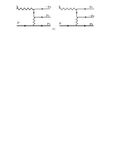
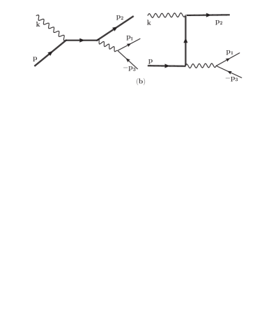
Figure 1: The Feynman diagrams for the process (1). Diagrams (a) are called the Borsellino diagrams, and diagrams (b) are the Compton-type diagrams.

The applied method is the following: We calculate first the double differential cross section over the invariant variables $s_{1}$ and $u=(k-p_{2})^{2}$. Next, we find the kinematical region, in terms of these variables, where the single-photon amplitudes give a comparable or larger contribution with respect to the double-photon amplitudes of the Borsellino diagrams in Fig. 1(a). This region can be delimited by excluding the large $|u|$ values with appropriate cuts. Then, we perform an integration over the variable $u$ in this restricted region and include the effect due to the DP contribution.

II.1 Kinematics

To describe the process (1) we introduce the following set of invariant variables Byckling and Kajantie (1972):

$$s= (k+p)^{2}=(p_{1}+p_{2}+p_{3})^{2},\ s_{1}=(p_{1}+p_{3})^{2}=(k+p-p_{2})^{2},$$

$$s_{2}= (p_{2}+p_{3})^{2}=(k+p-p_{1})^{2},$$

$$t_{1}= (k-p_{1})^{2}=(p_{2}+p_{3}-p)^{2},\ t_{2}=(p-p_{2})^{2}=(p_{1}+p_{3}-k)^{2}.$$

In terms of these variables, we have:

$$2(k\,p_{2})= s-s_{1}+t_{2}-M^{2},2(k\,p)=s-M^{2},\ 2(k\,p_{1})=m^{2}-t_{1},$$ (3)

$$2(k\,p_{3})= s_{1}+t_{1}-t_{2}-m^{2},\ u=2M^{2}-s+s_{1}-t_{2},$$

$$2(p\,p_{1})= s-s_{2}+t_{1},\ 2(p\,p_{2})=2M^{2}-t_{2},\ 2(p\,p_{3})=s_{2}-t_{1}+t_{2}-M^{2},$$

$$2(p_{1}\,p_{3})= s_{1}-2m^{2},\ 2(p_{2}\,p_{3})=s_{2}-M^{2}-m^{2},\ 2(p_{1}\,p_{2})=s-s_{1}-s_{2}+m^{2},$$

where $M~{}(m)$ is the mass of the initial (created) lepton.

For back-to-back events azimuthal symmetry applies and the phase space of the final particles can be written as Byckling and Kajantie (1972):

$$d\,R_{3}=\frac{d^{3}p_{1}}{2\,E_{1}}\,\frac{d^{3}p_{2}}{2\,E_{2}}\,\frac{d^{3}p_{3}}{2\,E_{3}}\,\delta(k+p-p_{1}-p_{2}-p_{3})=\frac{\pi}{16(s-M^{2})}\frac{dt_{1}\,dt_{2}\,ds_{1}\,ds_{2}}{\sqrt{-\Delta}}\,,$$ (4)

where $\Delta$ is the Gramian determinant. The limits of integration are defined by the condition of the positiveness of $(-\Delta).$ In Ref. Gakh et al. (2018) these limits have been obtained for the triplet production process where the masses of all leptons are equal. Similarly, we obtain for the considered reactions

$$t_{1-}<t_{1}<t_{1+}\,,\ \ \ t_{1\pm}=\frac{A\pm 2\sqrt{B}}{(s-s_{1})^{2}-2(s+s_{1})M^{2}+M^{4}}\,,$$ (5)

where

$$A = \left\{-M^{4}s_{1}+s_{1}s_{2}(s_{1}-t_{2})+s^{2}t_{2}+M^{2}\left[s_{1}^{2}+s_{1}s_{2}+s(s_{1}-t_{2})+s_{2}t_{2}\right]-\right.$$

$$\left.s\left[s_{2}t_{2}+s_{1}(s_{2}+t_{2})\right]+m^{2}\left[M^{4}+s(s-s_{1})+(s+s_{1})t_{2}-M^{2}(2s+3s_{1}+t_{2})\right]\right\}\,,$$

$$B = \left[st_{2}(s-s_{1}+t_{2})+M^{2}(s_{1}^{2}-2st_{2}-s_{1}t_{2})+M^{4}t_{2}\right]\times\left[m^{2}M^{4}+m^{4}s_{1}-m^{2}M^{2}(2s+s_{1})+\right.$$

$$\left.\ \ \ m^{2}(s^{2}-ss_{1}-2s_{1}s_{2})+M^{2}s_{1}(s-s_{2})+s_{1}s_{2}(-s+s_{1}+s_{2})\right]\,.$$

At fixed $s_{1}$ and $t_{2}$, we have $s_{2-}<s_{2}<s_{2+}$ where

$$s_{2\pm}=\displaystyle\frac{2m^{2}+M^{2}+s-s_{1}\pm\lambda_{1}\sqrt{1-\displaystyle\frac{4m^{2}}{s_{1}}}}{2}\,,\lambda_{1}=\sqrt{(s-s_{1})^{2}-2M^{2}(s+s_{1})+M^{4}}\,.$$ (6)

The corresponding range for $t_{2}$, $t_{2-}<t_{2}<t_{2+}$ and for $s_{1}$, $4m^{2}<s_{1}<(\sqrt{s}-M)^{2}$, is limited by the curves

$$t_{2\pm}=\frac{1}{2s}\left[C\pm\lambda_{1}(M^{2}-s)\,\right]\,,\ C=s_{1}(s+M^{2})-(s-M^{2})^{2}\,.$$ (7)

Furthermore, it is preferred to use the variable $u$ instead of $t_{2}$ because one of the Compton-type diagrams has a pole behavior precisely in the $u$ channel. The kinematical region ($s_{1},u$) is shown in Fig. 2, where:

$$u_{\pm}=\frac{1}{2s}\left[\bar{C}\pm\lambda_{1}(s-M^{2})\,\right]\,,\ \bar{C}=M^{4}+M^{2}(2s-s_{1})-s(s-s_{1})\,.$$ (8)

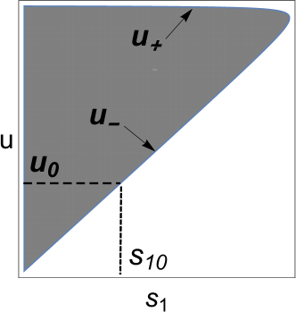
Figure 2: Kinematical region for $(s_{1},u)$. The quantity $s_{10}$ is the solution of the equation $u_{0}=u_{-}$, where $u_{0}$ is the negative cut parameter.

II.2 Calculation of the QED cross section

In the case of unpolarized particles, we have to average over (to sum over) the polarization states of the initial (final) particles. The differential cross section can be written in the form

$$d\sigma=\frac{1}{4}\,\frac{e^{6}}{4(k\,p)\,(2\pi)^{5}}\,\sum_{pol}|M|^{2}\,dR_{3}\,,$$ (9)

where $M$ is the matrix element of the process (1):

$$\sum_{pol}|M|^{2}=|M_{b}|^{2}+|M_{c}|^{2}+2{\cal Re}\big{(}M_{b}M^{*}_{c}\big{)},\$$ (10)

and the index $b\,\,(c)$ corresponds to the Borsellino (the Compton-type) diagrams.

The double differential cross section, as a function of the variables $s_{1}$ and $t_{2}$ [or the $(s_{1},t_{2})$ distribution], is

$$\frac{d\,\sigma}{d\,s_{1}\,d\,t_{2}}=\frac{\alpha^{3}}{64\,\pi(s-M^{2})^{2}}\int\int\frac{d\,s_{2}\,d\,t_{1}}{\sqrt{-\Delta}}\sum_{pol}|M|^{2}\,.$$ (11)

The calculation of the matrix element squared (10) gives:

$$|M_{b}|^{2} = \displaystyle\frac{8}{t_{2}^{2}}\left\{\displaystyle\frac{8d^{2}m^{2}}{d_{3}^{2}}+t_{2}^{2}\left[\left(\frac{1}{d_{3}^{2}}+\displaystyle\frac{1}{d_{1}^{2}}\right)m^{2}-\displaystyle\frac{2M^{2}}{d_{1}d_{3}}-\displaystyle\frac{2}{d_{3}}\left(\displaystyle\frac{d}{d_{1}}+1\right)\right]+\right.$$

$$8(\text{pp}_{3})^{2}\left[\left(\frac{1}{d_{3}}+\frac{1}{d_{1}}\right){}^{2}m^{2}-\frac{t_{2}}{d_{1}d_{3}}\right]+$$

$$4(\text{pp}_{3})\left[t_{2}\left(-m^{2}\left(\frac{1}{d_{3}}+\frac{1}{d_{1}}\right)^{2}-\frac{1}{d_{1}}+\frac{2d}{d_{1}d_{3}}+\frac{1}{d_{3}}\right)-\frac{4d}{d_{3}}\left(\frac{1}{d_{3}}+\frac{1}{d_{1}}\right)m^{2}+\frac{t_{2}^{2}}{d_{1}d_{3}}\right]+$$

$$t_{2}\left[2\left(\frac{1}{d_{3}}+\frac{1}{d_{1}}\right)^{2}m^{4}+2\left(\frac{1}{d_{3}}+\frac{1}{d_{1}}\right)^{2}m^{2}M^{2}+4\left(\frac{1}{d_{3}}+\frac{1}{d_{1}}\right)\left(\frac{d}{d_{3}}-1\right)m^{2}-\right.$$

$$\left.\left.4\left(\frac{1}{d_{3}}+\frac{1}{d_{1}}\right)M^{2}-2\left(\frac{d_{1}}{d_{3}}+\frac{2d}{d_{1}}\left(\frac{d}{d_{3}}-1\right)+\frac{d_{3}}{d_{1}}\right)\right]-4\left(\frac{d_{1}}{d_{3}}+\frac{d_{3}}{d_{1}}\right)M^{2}-\frac{t_{2}^{3}}{d_{1}d_{3}}\right\}\,,$$

$$|M_{c}|^{2} = |M_{b}|^{2}(p\leftrightarrow-p_{3},p_{1}\leftrightarrow p_{2},m\leftrightarrow M)\,,\ d_{i}=(kp_{i}).$$

On the level of the full differential cross section, the interference of $M_{c}$ and $M_{b}$ contributes also, but in the experimental setup considered in this paper, where only the scattered $\ell_{i}$ lepton is recorded, it vanishes due to the Furry theorem Furry (1937).

Introducing the short notation:

$$\frac{\pi}{64\,(s-M^{2})}\int\limits_{s_{2-}}^{s_{2+}}d\,s_{2}\int\limits_{t_{1-}}^{t_{1+}}d\,t_{1}\displaystyle\frac{W}{\sqrt{-\Delta}}\equiv\overbrace{W},$$

and applying the relation (3) between the variables $t_{2}$ and $u$, we have

$$\overbrace{|M_{c}|^{2}} = \displaystyle\frac{2\pi^{2}\sqrt{1-\displaystyle\frac{4m^{2}}{s_{1}}}(2m^{2}+s_{1})}{3(M^{2}-s)^{2}s_{1}^{3}(M^{2}-u)}\times$$

$$\left\{-4M^{6}+(s-s_{1}+u)(5M^{4}-2s_{1}^{2}+su)-M^{2}\left[s^{2}-4s_{1}^{2}+s_{1}u+u^{2}+s(s_{1}+6u)\right]\right\}\,,$$

$$\overbrace{|M_{b}|^{2}} =\frac{4\pi^{2}}{\left(M^{2}-s\right)\left(2M^{2}-s+s_{1}-u\right)^{2}}\times$$ (13)

$$\left\{\ln\left(\frac{\sqrt{s_{1}-4m^{2}}+\sqrt{s_{1}}}{2m}\right)\left[\frac{4s_{1}[s_{1}^{2}-2m^{2}(2m^{2}-3s_{1})](M^{2}-s)^{2}}{(-2M^{2}+s+u)^{4}}-\right.\right.$$

$$\frac{4(M^{2}-s)[2m^{2}\left(2m^{2}(M^{2}-s-s_{1})+s_{1}(-5M^{2}+5s+3s_{1})\right)+s_{1}^{2}\left(-2M^{2}+2s+s_{1}\right)]}{\left(2M^{2}-s-u\right)^{3}}-$$

$$\frac{2[-4m^{4}+m^{2}(-8M^{2}+8s+2s_{1})+(M^{2}-s)^{2}+s_{1}(-M^{2}+3s+2s_{1})]}{-2M^{2}+s+u}+$$

$$\frac{1}{(-2M^{2}+s+u)^{2}}2[2m^{2}\left(4(M^{2}-s)^{2}+s_{1}(10s+s_{1}-8M^{2})-2m^{2}(2s+s_{1})\right)+$$

$$s_{1}\left(3(M^{2}-s)^{2}+s_{1}(4s+s_{1}-2M^{2})\right)]+2M^{2}+s+3s_{1}-u\bigg{]}-$$

$$\sqrt{1-\frac{4m^{2}}{s_{1}}}\bigg{[}-\frac{4(M^{2}-s)[m^{2}s_{1}(M^{2}-s-s_{1})+2s_{1}^{2}(2M^{2}-2s-s_{1})]}{(-2M^{2}+s+u)^{3}}+$$

$$\frac{4s_{1}^{2}(M^{2}-s)^{2}(m^{2}+2s_{1})}{(-2M^{2}+s+u)^{4}}+$$

$$\frac{s_{1}[2m^{2}(2s+s_{1})+9(M^{2}-s)^{2}+2s_{1}(-6M^{2}+8s+s_{1})]}{(-2M^{2}+s+u)^{2}}-$$

$$\frac{s_{1}(2m^{2}-5M^{2}+9s+4s_{1})+(M^{2}-s)^{2}}{-2M^{2}+s+u}+\frac{1}{2}(2M^{2}+s+5s_{1}-u)\bigg{]}\bigg{\}}\,.$$

Following Eq. (11) and the definition of the quantity $\overbrace{W}$, the double differential cross section can be written as

$$\frac{d\sigma}{d\,s_{1}\,d\,u}=\frac{\alpha^{3}}{\pi^{2}(s-M^{2})}\overbrace{\sum_{pol}|M|^{2}}\,,$$ (14)

where $\sum_{pol}|M|^{2}$ is defined by Eq. (10). To measure the differential cross section $d\,\sigma/(ds_{1}du),$ it is sufficient to detect the final muon 4-momenta.

The integration of the double differential cross section (14) with respect to the variable $u$ in the limits $u_{-}<u<u_{+}$ gives

$$\frac{d\sigma_{c}}{ds_{1}} = \displaystyle\frac{\alpha^{3}\sqrt{1-\displaystyle\frac{4m^{2}}{s_{1}}}(2m^{2}+s_{1})}{3\pi s_{1}^{2}(s-M^{2})^{3}}\left\{\frac{\lambda_{1}[M^{6}-M^{4}(s+s_{1})+M^{2}s(15s+2s_{1})+s^{2}(s+7s_{1})]}{2s^{2}}-\right.$$ (15)

$$\left.[3M^{4}+M^{2}(6s-2s_{1})-s^{2}+2(s-s_{1})s_{1}]\ln\left[\frac{(M^{2}+s-s_{1}+\lambda_{1})^{2}}{4M^{2}s}\right]\right\}\,,$$

$$\frac{d\sigma_{b}}{d\,s_{1}} = \displaystyle\frac{2\alpha^{3}}{\pi(s-M^{2})}\left\{\displaystyle\frac{2\lambda_{1}\sqrt{1-\displaystyle\frac{4m^{2}}{s_{1}}}}{3s_{1}^{3}(M^{2}-s)^{2}}\right.$$

$$\left[m^{2}[17(M^{2}-s)^{2}+2s_{1}(4M^{2}-2s+s_{1})]+s_{1}[7(M^{2}-s)^{2}+s_{1}(4M^{2}-2s+s_{1})]\bigg{]}+\right.$$

$$\frac{1}{s_{1}^{4}(s-M^{2})}\Bigg{[}s_{1}\sqrt{1-\displaystyle\frac{4m^{2}}{s_{1}}}\bigl{[}2m^{2}[2(M^{2}-s)^{2}+s_{1}(6M^{2}-2s+s_{1})]$$

$$+s_{1}[(M^{2}-s)^{2}+s_{1}(5M^{2}-s)]\bigr{]}+2\bigl{[}4m^{4}[2(M^{2}-s)^{2}+s_{1}(6M^{2}-2s+s_{1})]-$$

$$-2m^{2}s_{1}[2(M^{2}-s)^{2}+s_{1}(6M^{2}-2s+s_{1})]-$$

$$s_{1}^{2}[(M^{2}-s)^{2}+s_{1}(3M^{2}-s)]\bigr{]}\ln\left(\frac{\sqrt{s_{1}-4m^{2}}+\sqrt{s_{1}}}{2m}\right)\Bigg{]}\times$$

$$\ln\left(\frac{\left(\lambda_{1}-M^{2}+s+s_{1}\right)^{2}}{4ss_{1}}\right)-$$

$$\frac{2\lambda_{1}}{3s_{1}^{4}(M^{2}-s)^{2}}\bigl{[}-4m^{4}[17(M^{2}-s)^{2}+2s_{1}(4M^{2}-2s+s_{1})]+$$

$$6m^{2}s_{1}(M^{2}-s)(7M^{2}-7s+2s_{1})+$$

$$s_{1}^{2}[8(M^{2}-s)^{2}+s_{1}(5M^{2}-s+2s_{1})]\bigr{]}\times\ln\left(\frac{\sqrt{s_{1}-4m^{2}}+\sqrt{s_{1}}}{2m}\right)+$$

$$\frac{1}{2s_{1}^{4}(s-M^{2})}\left[s_{1}\sqrt{1-\frac{4m^{2}}{s_{1}}}\bigl{[}4m^{2}[2(M^{2}-s)^{2}+s_{1}(6M^{2}-2s+s_{1})]+\right.$$

$$+s_{1}[2(M^{2}-s)^{2}+s_{1}(10M^{2}-2s+s_{1})]\bigr{]}+$$

$$2(8m^{4}-4m^{2}s_{1}-s_{1}^{2})[2(M^{2}-s)^{2}+s_{1}(6M^{2}-2s+s_{1})]\times$$

$$\left.\left.\ln\left(\frac{\sqrt{s_{1}-4m^{2}}+\sqrt{s_{1}}}{2m}\right)\right]\ln\left[\frac{[M^{4}+\lambda_{1}(M^{2}-s)-M^{2}(2s+s_{1})+s(s-s_{1})]^{2}}{4M^{2}ss_{1}^{2}}\right]\right\}\,.$$

We can also write a more complicated analytical expression for $d\sigma/ds_{1}$ accounting for the restriction on the variable $u$. The corresponding result is given in the Appendix.

In the limiting case $s\gg(s_{1},M^{2})\gg m^{2}$, which applies for electron-positron pair production, these expressions are essentially simplified, namely

$$\frac{d\sigma_{c}}{d\,s_{1}} = \frac{\alpha^{3}}{3\,\pi\,s\,s_{1}}\left[\frac{1}{2}+\frac{17\,M^{2}+2\,s_{1}}{2\,s}+\left(1-\frac{3\,M^{2}+2\,s_{1}}{s}\right)\ln{\frac{s}{M^{2}}}\right]\,,$$

$$\frac{d\sigma_{b}}{d\,s_{1}} = \frac{2\,\alpha^{3}}{\pi\,s_{1}^{2}}\left\{\ln{\frac{s_{1}}{m^{2}}}\ln{\frac{s^{2}}{s_{1}\,M^{2}}}-\frac{8}{3}\ln{\frac{s_{1}}{m^{2}}}-\ln{\frac{s^{2}}{s_{1}\,M^{2}}}+\frac{14}{3}+\right.$$

$$\left.\frac{1}{s}\left[-s_{1}\,\ln{\frac{s_{1}}{m^{2}}}\ln{\frac{s^{2}}{s_{1}M^{2}}}+(s_{1}-2M^{2})\ln{\frac{s_{1}}{m^{2}}}+s_{1}\,\ln{\frac{s^{2}}{s_{1}M^{2}}}-4s_{1}+2M^{2}\right]\right\}\,.$$

Eqs. (15) and (II.2) hold for particles with arbitrary masses. They can be applied to the reactions:

$$\gamma+e^{-}\to\mu^{+}\mu^{-}+e^{-},\ \gamma+e^{-}\to\tau^{+}\tau^{-}+e^{-},\ \gamma+\mu^{-}\to\tau^{+}\tau^{-}+\mu^{-},$$

and the asymptotic formulas, in the limit $s\gg(s_{1},\,m^{2})\gg M^{2},$ valid for muon pair production, become:

$$\frac{d\sigma_{c}}{d\,s_{1}} = \frac{\alpha^{3}}{6\pi\,s\,s_{1}}(2+y)\sqrt{1-y}\left[\frac{1}{2}+x_{1}+(1-2x_{1})\ln{\frac{s}{M^{2}}}\right]\,,\ x_{1}=\frac{s_{1}}{s}\,,\ y=\frac{4m^{2}}{s_{1}}\,,$$

$$\frac{d\sigma_{b}}{d\,s_{1}} = \frac{2\,\alpha^{3}}{\pi\,s_{1}^{2}}\left\{\left[(2+2y-y^{2})L-(1+y)\sqrt{1-y}\right](1-x_{1})\ln{\frac{s^{2}}{M^{2}s_{1}}}+\right.$$

$$\left.\left[\frac{17}{6}y^{2}-7y-\frac{16}{3}+x_{1}\left(2+5y-\frac{3}{2}y^{2}\right)\right]\,L+\sqrt{1-y}\left[\frac{14}{3}+\frac{17}{6}y-x_{1}\left(4+\frac{3}{2}y\right)\right]\right\},$$

$$L = \ln{\frac{\sqrt{s_{1}}+\sqrt{s_{1}-4m^{2}}}{2m}}\,.$$

III Analysis of the dark photon signal

We have to estimate first the QED background in order to find the kinematical conditions where the cross section $d\sigma_{c}/ds_{1}$ exceeds $d\sigma_{b}/ds_{1},$ because in our work, the DP signal is related to a modification of the Compton-type diagrams. We perform the following calculations for $e^{+}e^{-}$ pair creation.

It is well known that at photon energies larger than 10 MeV, the main contribution to the cross section of the tripletlike processes arises from the Borsellino diagrams due to the events at small values of $t_{2}$ Boldyshev et al. (1994).

In Fig. 3, we show : (a) the differential cross section, i.e., the sum of (15) and (II.2) contributions as a function of the dimensionless variable $x_{1}=s_{1}/s$ at fixed $s$, and (b) the ratio of the Compton-type diagrams contribution to the Borsellino ones as a function of $s_{1}$,

$$R^{c}_{b}=\frac{d\sigma_{c}}{d\sigma_{b}}\,,\$$

at different colliding energies: $s=$6, 30, 60 GeV², provided that the whole kinematical region ($s_{1},u$) is allowed. We see that in a wide, physically interesting range of variable $s_{1},$ the quantity $R^{c}_{b}(s_{1})$ is rather small (does not exceed 2$\cdot$10^-2) and it is obvious that, in the case of the nonlimited phase space, the Borsellino contribution leads to a very large QED background for searching for a small DP signal which modifies the Compton-type contribution only.

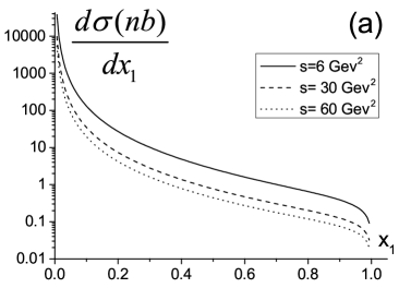
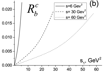
Figure 3: (a) Differential cross section of the process $\gamma+\mu^{-}\to e^{+}e^{-}+\mu^{-},$ as a function of $x_{1}=s_{1}/s$ for fixed values of the variable $s$, calculated with Eqs. (15) and (II.2); (b) Ratio of the contributions to the cross section of the Compton-type diagrams to the Borsellino ones as a function of the $e^{+}e^{-}$ invariant mass squared,.

To find the kinematical region where the signal over background ratio is maximized, we analyze the double $(s_{1},u)$ distribution separately for the Compton and Borsellino contributions, using relations (II.2) and (13), and the results are presented in Fig. 4, where we plot the corresponding double differential cross sections and from which one can easily determine the regions where the Compton contribution exceeds the Borsellino one. We see that the contribution due to the Compton-type diagrams increases with decrease of both variables, $s_{1}$ and $|u|$, whereas the contribution of the Borsellino diagrams indicates just the opposite behaviour. Since we have to scan $s_{1}-$distribution, we can restrict the ($s_{1},u$) region by cutting the large values of $|u|$ in order to reach our goal.

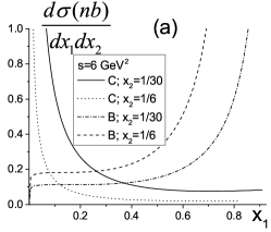
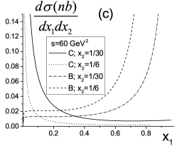
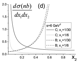
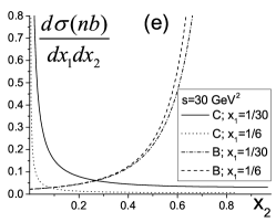
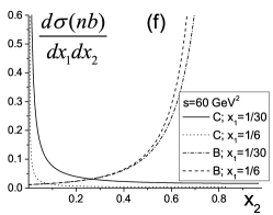
Figure 4: Double differential cross section for the reaction $\gamma+\mu^{-}\to e^{+}e^{-}+\mu^{-}.$ In the first row it is given as a function of $x_{1}=s_{1}/s$ for fixed values of the variable $x_{2}=|u|/s$: for the Compton-type diagrams $x_{2}=1/30$ (solid line) and $x_{2}=1/6$ (dotted line), for the Borsellino diagrams $x_{2}=1/30$ (dash-dotted line) and $x_{2}=1/6$ (dashed line); and for different values of the total energy squared $s$: $s=6$ GeV² (a), $s=30$ GeV² (b), and $s=60$ GeV² (c); - in the second row it is given as a function of $x_{2}$ for fixed values of the variable $x_{1}$: for the Compton-type diagrams $x_{1}=1/30$ (solid line) and $x_{1}=1/6$ (dotted line), for the Borsellino diagrams $x_{1}=1/30$ (dash-dotted line) and $x_{1}=1/6$ (dashed line), and for different values of the total energy squared $s:$   $s=6$ GeV² (a), $s=30$ GeV² (b), and $s=60$ GeV² (c).

As one can see from the curves in Fig. 4, there is a large region of variables $u$ and $s_{1}$ where the Compton contribution exceeds the Borsellino one, and it indicates that measurements should be preferentially performed in this region to detect the DP signal in form of a resonance in the single-photon intermediate state. The corresponding regions for the different reactions are shown in Fig. 5.

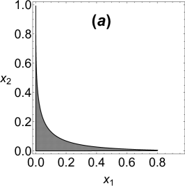
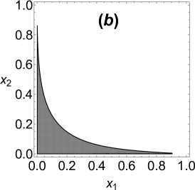
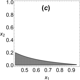
Figure 5: Kinematical region where the Compton contribution to the double differential cross section exceeds the Borsellino contribution, at $s$=30 GeV²: (a) for the process $\gamma+\mu^{-}\to e^{+}e^{-}+\mu^{-},$ (b) for the process $\gamma+e^{-}\to\mu^{+}\mu^{-}+e^{-},$ and (c) for the processes $\gamma+e^{-}(\mu^{-})\to\tau^{+}\tau^{-}+e^{-}(\mu^{-}).$

To reduce the Borsellino contribution, we suggest to remove the events with small values of the variable $|t_{2}|$ (or with large values of $|u|$) by the kinematical cut:

$$u\,>u_{0},$$ (17)

where $u_{0}$ is a negative parameter that may take different values in the numerical calculations below. We can perform the integration over the variable $u$ and derive an analytical result for the $s_{1}$ distribution even in the restricted phase space given by Eq. (17). In this case, the region of the variables $u$ and $s_{1}$ is shown in Fig. 2, where the quantity $s_{10}$ is the solution of the equation $u_{0}=u_{-}$ and reads

$$s_{10}=\frac{(M^{4}-su_{0})(2M^{2}-s-u_{0})}{(M^{2}-u_{0})(s-M^{2})}\,,\ u_{0}<\tilde{u}\,,\ \tilde{u}=M\left(\frac{M^{2}}{\sqrt{s}}+M-\sqrt{s}\right)\,.$$ (18)

Note that the solution given by Eq. (18) is the same also for the equation $u_{0}=u_{+}$, with

$$u_{0}>\tilde{u}\,,\ \big{[}4m^{2}<s_{1}<s_{10}\,,\ u_{0}<u<u_{+}\big{]}\,.$$

Two subregions can be delimited:

$$\left[4m^{2}<s_{1}<s_{10},\,u_{0}<u<u_{+}\right]\,;\ \left[s_{10}<s_{1}<(\sqrt{s}-M)^{2}\,,\ u_{-}<u<u_{+}\right]\,.$$

The event selection, under the constraint (17) (restricted phase space), decreases essentially the Borsellino contribution, whereas the Compton-type contribution decreases weakly. Their ratio

$$\widetilde{R}^{c}_{b}=\frac{d\sigma_{c}(u>u_{0})}{d\sigma_{b}(u>u_{0})},$$ (19)

in the limited phase space is shown in Fig. 6, to be compared to the ratio $R^{c}_{b}$.

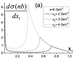
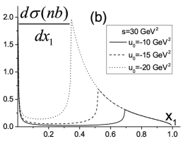
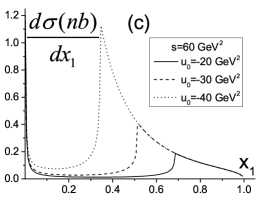
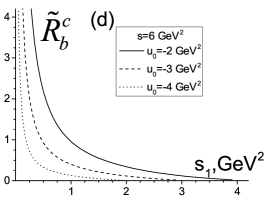
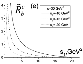
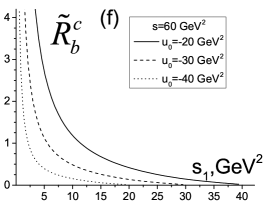
Figure 6: Differential cross section of the process $\gamma+\mu^{-}\to e^{+}e^{-}+\mu^{-}$, as a function of the $e^{+}e^{-}$ invariant mass squared, for the sum of the Compton-type (15) and the Borsellino (II.2) contributions, with the constraint (17), is shown for $s=6$ GeV² (a), $s=30$ GeV² (b), and $s=60$ GeV² (c), and for $u_{0}$=-2 GeV² (solid line), $u_{0}$=-3 GeV² (dashed line) and $u_{0}$=-4 GeV² (dotted line). The corresponding ratio of the Compton-type (15) to the Borsellino contributions is shown in the insets (d-f).

The differential cross section of the process $\gamma+\mu^{-}\to e^{+}e^{-}+\mu^{-}$ is illustrated in Figs. 6(a-c) taking into account all the contributions in the matrix element squared (10) and the constraint (17). This cross section is plotted as a function of the dimensionless variable $x_{1}$, for different values of $u_{0}$ . Figure 6 shows a steep decrease of this cross section, whereas $s$ and $u_{0}$ increase. The ratio Compton-type contribution to the Borsellino one for the corresponding kinematics is shown in Figs. 6(d-f). We apply the approach developed in Ref. Gakh et al. (2018) (see also Bjorken et al. (2009); Chiang and Tseng (2017)) to obtain the constraints on the possible values of DP parameters $\epsilon$ and $M_{A^{\prime}}$ for a fixed event number $N$ and standard deviation $\sigma.$ The effective QED and DP Lagrangian Bjorken et al. (2009)

$$\mathcal{L}=\mathcal{L}_{QED}+\displaystyle\frac{1}{2}\epsilon F^{\mu\nu}F^{\prime}_{\mu\nu}-\displaystyle\frac{1}{4}F^{{}^{\prime}\mu\nu}F^{\prime}_{\mu\nu}+M^{2}_{A^{\prime}}A^{{}^{\prime}\mu}A^{\prime}_{\mu}$$ (20)

ensures the propagation of the fields $A_{\mu}$ and $A^{\prime}_{\mu}$ and generates the interaction of the DP with the SM leptons in the form

$$e\epsilon\bar{\psi}_{j}(x)\gamma^{\mu}\psi_{j}(x)A^{\prime}_{\mu},\ \ j=e,\mu,\tau$$

due to the kinetic mixing effect [the second term in the rhs of Eq. (20)]. We assume that selected values of the $\ell^{+}_{j}~{}\ell^{-}_{j}$ invariant mass fall in the energy region

$$M_{A^{\prime}}-\delta m/2<\sqrt{s_{1}}<M_{A^{\prime}}+\delta m/2\,,$$

where $\delta m$ is the experimental resolution for the invariant mass, $i.e.$, the bin width containing the events of the possible signal.

The DP modifies the Compton-type matrix element by the spin-one particle Breit-Wigner propagator in such a way that its contribution into the cross section reads

$$d\sigma_{A^{\prime}}=\frac{\epsilon^{2}s_{1}[2(s_{1}-M^{2}_{A^{\prime}})+\epsilon^{2}s_{1}]d\sigma_{c}}{D(s_{1})}\,,\ D(s_{1})=(s_{1}-M^{2}_{A^{\prime}})^{2}+M^{2}_{A^{\prime}}\Gamma^{2}\,,$$ (21)

where the DP width $\Gamma$ is defined by its decays to SM lepton pairs

$$\Gamma(\gamma\,^{\prime}\to{\ell}^{+}{\ell}^{-})=\epsilon^{2}\,\frac{\alpha}{3M_{A^{\prime}}^{2}}(M_{A^{\prime}}^{2}+2m_{\ell}^{2})\sqrt{M_{A^{\prime}}^{2}-4m_{\ell}^{2}}\,\,\Theta(M_{A^{\prime}}-2m_{l})=\epsilon^{2}\,\Gamma_{0},$$ (22)

where $m_{\ell}$ is the SM lepton mass and $\Theta(x)$ is the Heaviside $\Theta$ function. The term $2(s_{1}-M^{2}_{A^{\prime}})$ in the numerator of $d\sigma_{A^{\prime}}$ in Eq. (21) describes the QED-DP interference, whereas the term $\epsilon^{2}\,s_{1}$ corresponds to the pure DP contribution.

In our numerical calculations, where $e^{+}e^{-}$ or $\mu^{+}\mu^{-}$ pairs are created, we restrict ourselves to the analysis of a light DP signal with mass $M_{A^{\prime}}<1$ GeV. Then, the decay $A^{\prime}\to\tau^{+}\tau^{-}$ is forbidden and, therefore, $m_{\ell}$ in (22) is the electron or the muon mass.

Bearing in mind that

$$\Gamma\ll\delta m\ll M_{A^{\prime}}\,,$$

we can apply the narrow resonance approximation and write:

$$\left[D(s_{1})\right]^{-1}=\frac{\pi}{M_{A^{\prime}}\,\epsilon^{2}\Gamma_{0}}\delta(s_{1}-M_{A^{\prime}}^{2})\,.$$

Applying Chiang and Tseng (2017); Gakh et al. (2018):

$$\sigma d\,\sigma_{Q}=\sqrt{N}d\,\sigma_{A^{\prime}}\,,$$ (23)

one obtains, by integrating both sides over the bin range

$$\epsilon^{2}=\frac{2\,\sigma}{\pi\sqrt{N}}\frac{\delta m\Gamma_{0}}{M_{A^{\prime}}^{2}}\frac{d\sigma_{Q}(M_{A^{\prime}}^{2})}{d\sigma_{c}(M_{A^{\prime}}^{2})}\,,$$ (24)

where $d\sigma_{Q}$ is the total QED contribution.

Equation (24) defines the constraints on the parameters $\epsilon^{2},M_{A^{\prime}}^{2}$ and the number of the detected events $N$ for a given standard deviation $\sigma.$ The effect due to the QED-DP interference relative to the pure DP contribution can be easily estimated by integrating Eq. (21) at $d\sigma(s_{1}=M^{2}_{A^{\prime}})$ over the above described bin range, giving

$$\frac{4\delta m\Gamma_{0}}{\pi M^{2}_{A^{\prime}}}\ll 1.$$

These constraints are illustrated below (Figs. 7-9) at $\sigma=2$ for the energy bin value $\delta m=1$ MeV. In our calculations we assume that there are three channels of the DP decays into SM leptons: $A^{\prime}\to e^{+}e^{-}$, $\mu^{+}\mu^{-}$, $\tau^{+}\tau^{-}$. The plots of $\epsilon^{2}$ versus $M_{A^{\prime}}$ for the reaction $\gamma+\mu^{-}\to e^{+}e^{-}+\mu^{-}$ are shown in Figs. 7, and 8 for $M_{A^{\prime}}<2M$ and $M_{A^{\prime}}>2M$, correspondingly. In the case of $e^{+}e^{-}$ pair production we restrict ourselves with the DP mass values $M_{A^{\prime}}<2m_{\tau}\ (m_{\tau}$ is the $\tau$ lepton mass) and, therefore, take into account DP decays into $e^{+}e^{-}$ and $\mu^{+}\mu^{-}$ when calculating the quantity $\Gamma_{0}.$ The plots for the $\gamma+\mu^{-}\to\tau^{+}\,\tau^{-}+\mu^{-}$ process are shown in Fig. 9. In this case, all three channels of DP decays contribute into $\Gamma_{0}.$

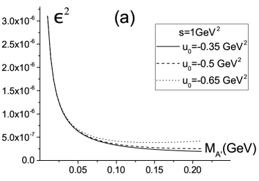
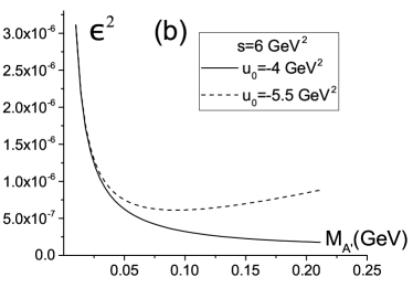
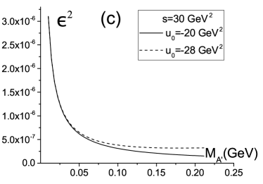
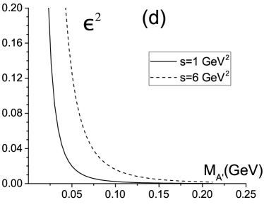
Figure 7: Constraints on the DP parameters in terms of $\epsilon^{2}$ as a function of $M_{A^{\prime}}$ for the conditions: $N=10^{4}$, $\sigma=2$, and $\delta m=1$ MeV, in the process $\gamma+\mu^{-}\to e^{+}e^{-}+\mu^{-}$, for $M_{A^{\prime}}<2M$, where only one channel of DP decay is allowed, for $s=1$ GeV² (a), $s=6$ GeV² (b), and $s=30$ GeV² (c). Different curves correspond to different values of $u_{0}$, i.e., different kinematical cuts, and represent the lower limit on the DP parameters in the case of no DP event detected. Inset (d) shows the ($\epsilon^{2}$, $M_{A^{\prime}})$ dependence for $s=1$ GeV² (solid line) and $s=6$ GeV² (dashed line) without kinematical cuts.

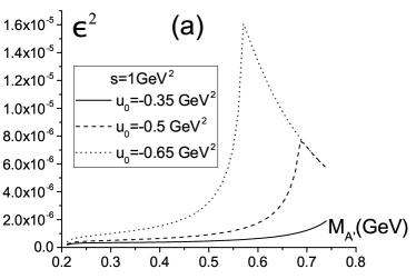
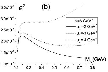
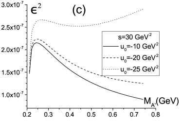
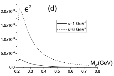
Figure 8: The same as in Fig.7 but in the region of greater DP masses, $M_{A^{\prime}}>2M$ where two channels are open for DP decays.

We can conclude that the kinematical limits to reduce the contribution of the Borsellino diagrams in the cross section increase essentially the sensitivity to the DP signal and should be implemented in the experimental event selection.

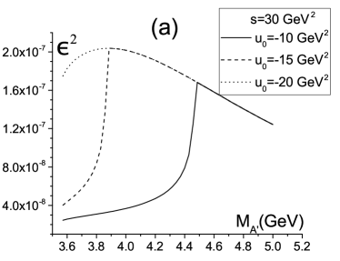
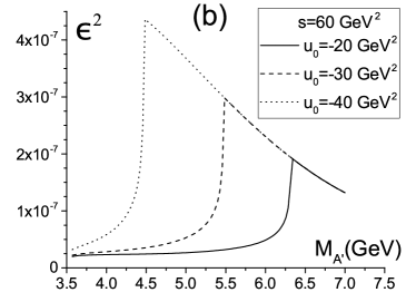
Figure 9: $\epsilon^{2}$ versus $M_{A^{\prime}}$ for the reaction $\gamma+\mu^{-}\to\tau^{+}\tau^{-}+\mu^{-}$, for $s=30$ GeV² (a) and $s=60$ GeV² (b). Different curves correspond to different values of $u_{0}$, i.e., different kinematical cuts.

The corresponding results of calculations for the reactions $\gamma+e^{-}\to\mu^{+}\,\mu^{-}+e^{-}$ and $\gamma+e^{-}\to\tau^{+}\,\tau^{-}+e^{-}$ are shown in Figs. 10 and 11. Again, in the case of $\mu^{+}\mu^{-}$ production, the limit $M_{A^{\prime}}<2m_{\tau}$ is applied.

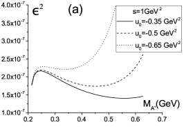
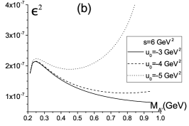
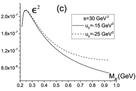
Figure 10: The same as in Figs. 8(a-c) but for the process $\gamma+e^{-}\to\mu^{+}\mu^{-}+e^{-}$.

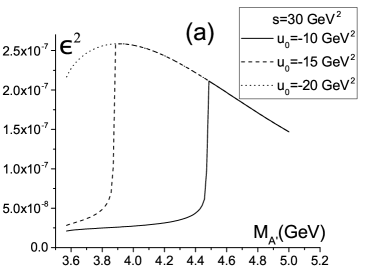
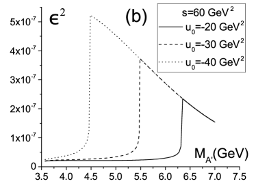
Figure 11: The same as in Fig. 9 but for the process $\gamma+e^{-}\to\tau^{+}\tau^{-}+e^{-}$.

For every point in the $(\epsilon^{2},M_{A^{\prime}})$ region (at a given values of $s$ ) below curves, $\sigma<2$ and above curves, $\sigma>2$. If the real $A^{\prime}$ signal corresponds, at least, to three (or more) standard deviations, then the quantities $\epsilon^{2}$ (at fixed $M_{A^{\prime}}$), when this signal can be recorded, increase by 1.5 times (or more) as compared with the corresponding points on the curves in Figs. 7-11. To be complete, we plot also in Fig.12 the possible $\epsilon^{2}$ and $M_{A^{\prime}}$ bounds which can be obtained in the triplet production process $\gamma+e^{-}\to e^{+}e^{-}+e^{-}$ for the DP masses enlarged up to 1 GeV values as compared with Ref.Gakh et al. (2018).

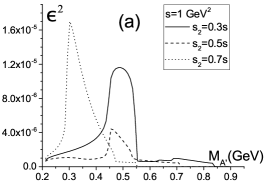
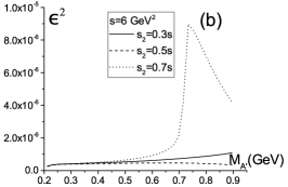
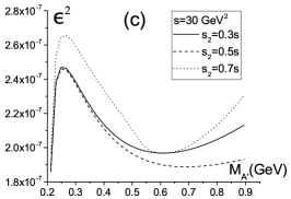
Figure 12: The $(\epsilon^{2},M_{A^{\prime}})$ bounds for the DP manifestation in the process $\gamma+e^{-}\to e^{+}e^{-}+e^{-}$ calculated by formulas of Ref. Gakh et al. (2018) but with corrected value of $\Gamma$ that takes into account decay $A^{\prime}\to\mu^{+}\mu^{-}$.

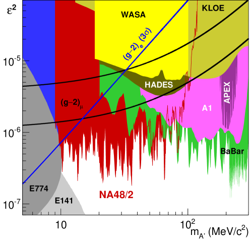
Figure 13: The NA48/2 preliminary upper limits at 90 $\%$ CL on the mixing parameter $\epsilon^{2}$ versus the DP mass $m_{A^{\prime}}$ Goudzovski (2015), compared to the other published exclusion limits from meson decay, beam dump and $e^{+}e^{-}$ collider experiments Lees et al. (2014). The results obtained in Refs. Davoudiasl et al. (2014) and Pospelov (2009) from the muon and electron $g-2$ factors are also shown.

It is easy to see from Eq. (24) that an increase of the energy bin value $\delta m$ decreases the sensitivity of the detection of the $A^{\prime}$ signal in the process (1). The reason is evident, because such an experimental device increases the QED background which is, in fact, proportional to $\delta m$ and leaves unchanged the number of events due to the DP signal in the narrow $A^{\prime}$ resonance. The dependence of the sensitivity on the DP mass $M_{A^{\prime}}$ is determined by the interplay of the $M_{A^{\prime}}$-dependences of $\Gamma_{0}$, $d\sigma_{Q}$ and $d\sigma_{c}$ entering in Eq. (24). This statement takes place also if we use the exact form of $D(s_{1})$ when integrating both sides of Eq. (23). Accounting for the kinematical restriction (17) increases essentially the sensitivity, due to the suppression of the QED background. To illustrate the corresponding effect, $\epsilon^{2}(M_{A^{\prime}})$ for the reaction $\gamma+\mu^{-}\to e^{+}e^{-}+\mu^{-}$ is also plotted without the kinematical cuts.

The number of the events $N$ in the denominator of the rhs of Eq. (24), in the frame of the described event selection, can be written with a good approximation as

$$N=\frac{2\delta mM_{A^{\prime}}}{s}\frac{d\sigma_{Q}}{dx_{1}}\Big{(}x_{1}=\frac{M_{A^{\prime}}^{2}}{s}\Big{)}L\cdot T\,.$$ (25)

that allows one to estimate the necessary integral luminosity $(L\cdot T)$ for collecting 10⁴ events. Taking values for $d\sigma_{Q}$ in the range $10^{-31}-10^{-34}$ cm^-2 (as it follows from the curves in Fig. 6 ) and values for $2\delta mM_{A^{\prime}}/s$ in the range 10^-3-10^-1, one finds the interval

$$L\cdot T\approx(10^{36}-10^{41})\ {\rm cm}^{-2}$$

at the considered values of $s$ between 1 and 60 GeV². The largest energies require the largest integral luminosity and vice versa. As concerns the radiative corrections to the QED contribution, they do not essentially change the ratio $\sigma_{Q}/\sigma_{c}$ entering Eq. (24) and cannot essentially change the curves in Figs. 7-11.

Let us compare the constraints on the parameter $\epsilon$ estimated in our paper with the ones obtained in various experiments (see Fig. 13). The A1 Collaboration at MAMI Merkel et al. (2011) measured the mass distribution of the reconstructed $e^{+}e^{-}$ pair in the reaction $e^{-}+^{181}Ta\to e^{-}+e^{-}+e^{+}+^{181}Ta$. The measured limit is $\epsilon^{2}<10^{-6}$ in the following range of DP masses: 210 MeV/$c^{2}$ $<m_{e^{+}e^{-}}<300$ MeV/$c^{2}$ to be compared to our estimation for the $\epsilon^{2}$ value in this DP mass range : $(1-2)\times 10^{-7}$. We suggest, instead, to measure the distribution over the invariant mass of the produced lepton pair in the reactions $\gamma+\mu^{-}\to e^{+}+e^{-}+\mu^{-}$ and $\gamma+e^{-}\to\mu^{+}+\mu^{-}+e^{-}$ (see Figs. 8-10). In the DP search with the KLOE detector at the DA$\Phi$NE $e^{+}e^{-}$ collider Babusci et al. (2014), the authors looked for a dimuon mass peak in the reaction $e^{+}e^{-}\rightarrow\mu^{+}\mu^{-}\gamma$, corresponding to the decay $A^{\prime}\rightarrow\mu^{+}\mu^{-}$. With an integrated luminosity of 239.3 pb^-1 (5.35$\times$10⁵ events), they set a 90$\%$ C.L. upper limit for the kinetic mixing parameter $\epsilon^{2}$ of 1.6$\times 10^{-5}$ to 8.5$\times 10^{-7}$ in the mass region 520 $<m_{A^{\prime}}<$980 MeV. Our estimation for this DP mass range is $\epsilon^{2}\leq 10^{-7}$ ($\gamma+\mu^{-}\to e^{+}+e^{-}+\mu^{-}$) and $\epsilon^{2}\leq(10^{-7}-6\cdot 10^{-8})$ ($\gamma+e^{-}\to\mu^{+}+\mu^{-}+e^{-}$). DP was searched as a maximum in the invariant mass distribution of $e^{+}e^{-}$ pairs originating from the radiative decays as e.g. $\phi\rightarrow\eta e^{+}e^{-}$ in the experiment Moskal et al. (2013). Only an upper limit was set with 90$\%$ C.L. on $\epsilon^{2}<1.7\times 10^{-5}$ for 30 $<M_{A^{\prime}}<$400 MeV and $\epsilon^{2}<8\times 10^{-6}$ for the subregion 50 $<M_{A^{\prime}}<$ 210 MeV. Our results are competitive also in these conditions: $\epsilon^{2}\leq 10^{-7}$ ($\gamma+\mu^{-}\to e^{+}+e^{-}+\mu^{-}$).

Some published exclusion limits on the DP parameter space from meson decay, beam dump and $e^{+}e^{-}$ collider experiments Lees et al. (2014) are presented in Fig. 13, readapted from Fig. 6 in Ref. Goudzovski (2015).

Let us summarize the advantages of the photoproduction reactions with different lepton flavors in the final state

1. In order to obtain the master bidimensional distribution $(s_{1},~{}u)$, it is sufficient to measure only the $\ell_{i}$ particle 4-momentum. The master distribution does not contain the interference between the Compton-type and the Borsellino diagrams, which simplifies essentially the theoretical analysis.

2. In order to suppress the background due to the Borsellino contribution it is sufficient to set a cut only in one invariant variable (if all final flavors are the same, one needs a cut in two variables).

3. The DP physical events are accumulated in a wide region of invariant variables, allowing one to reduce the necessary integral luminosity. In the case of triplet photoproduction, besides the two cuts on invariant variables mentioned above, the events must be selected at a fixed value of one (from two final) $e^{+}~{}e^{-}$ pair.

IV Conclusion

We investigated the direct detection of dark photon, one of the new particles that may possibly shed light on the nature and on the interaction of dark matter. The DP is mixed with the ordinary photon due to the effect of the kinetic mixing and it can, therefore, interact with the SM leptons. It is characterized by a mass $M_{A^{\prime}}$ and a small parameter $\epsilon$ describing the coupling strength relative the electric charge $e$.

We analyzed a possible way to detect a DP signal when its mass lies in the range between few MeV and few GeV. This mass region is presently accessible at the existing accelerators. The idea is to scan the distribution of the invariant mass squared of the $\ell^{+}_{j}\ell^{-}_{j}$ system, $s_{1}$, in the reactions $\gamma+\ell_{i}\to\ell^{+}_{j}\ell^{-}_{j}+\ell_{i}$ with $i\neq j$ and $i=e,\mu$; $j=e,\mu,\tau,$ where few tens MeV photons collide with high-energy electron or muon beams. Because of the interaction with SM leptons, DP appears as a narrow resonance in the $\ell^{+}_{j}\ell^{-}_{j}-$system over a background, and modifies the Compton-type diagrams by the Breit-Wigner term. Choosing processes with $i\neq j$ one avoids the ambiguity of the measurements arising from the final particle identity.

First, we calculated the double differential cross section with respect to the variables $s_{1}$, and $u$ and then derived the $s_{1}$ distribution after integration over the variable $u$. Note that to measure such double differential cross section it is sufficient to measure the four-momentum of the final lepton $\ell_{i}$.

The advantage of this reaction is that the background is of a pure QED origin and can be calculated exactly with the necessary precision.

In the case when all kinematically possible values of the variable $u$ are taken into account, a large QED background arises due to the contribution of the Borsellino diagrams, as illustrated in Fig. 3. To suppress this background, we analyzed the $(s_{1},u)$ distribution and identified the kinematical regions where the contribution of the Compton-type diagrams exceed the Borsellino ones (see Fig. 4.). The background contribution increases when the variables $s_{1}$ and $u$ decrease, whereas the DP signal has just the opposite behavior. Therefore we applied different cuts $(u>u_{0})$ to exclude the range of large values of $|u|$ (see Figs. 5 and 6).

Selecting the restricted $(s_{1},u)$ region, we estimated the constraints on the possible values of the parameters $\epsilon^{2}$ and $M_{A^{\prime}}$ for a given number of the detected events, $N=10^{4}$, and standard deviation $\sigma=2$ for all considered reactions (see Figs. 7 -11). Our results suggest that a convenient bin width containing all the events of the possible DP signal near $s_{1}=M_{A^{\prime}}$ could be $\delta m$= 1 MeV. Equation (24) determines the relation between $\epsilon^{2}$ and $M_{A^{\prime}}$ as a function of the parameters $N$, $\sigma$ and $\delta m$.

V Acknowledgments

Two of us (N.P.M. and M.I.K) acknowledge the hospitality of IRFU/DPhN, under the Paris-Saclay grant AAP-P2I-DARKPHI. This work was partially supported by the Ministry of Education and Science of Ukraine (project n. 0118U002031). The research was conducted in the scope of the IDEATE International Research Project (IRP). This work was partially supported by the ERASMUS+ program (code F PARIS 011).

VI Appendix

To obtain the $s_{1}$ distribution it is convenient to define the quantity

$$\int\frac{d\sigma_{i}}{ds_{1}du}du\equiv F_{i}(s,s_{1},u)\,,\ i=b,\,c.$$

Then we have;

$$F_{b}(s,s_{1},u)=\frac{\alpha^{3}}{\pi(s-M^{2})}\Biggl{\{}\frac{\sqrt{s_{1}-4m^{2}}}{\sqrt{s_{1}}}\Biggr{[}\frac{2(4m^{2}+s_{1})M^{2}}{(M^{2}-s)(-2M^{2}+s+u-s_{1})s_{1}}+$$

$$\frac{8(M^{2}-s)(m^{2}+2s_{1})}{3(-2M^{2}+s+u)^{3}}+\frac{4[(M^{2}-s+s_{1})m^{2}+2s_{1}^{2}]}{(-2M^{2}+s+u)^{2}s_{1}}+$$

$$\frac{2}{(M^{2}-s)(-2M^{2}+s+u)s_{1}^{2}}\big{[}2\left(2M^{4}-4(s-s_{1})M^{2}+2s^{2}+s_{1}^{2}-2ss_{1}\right)m^{2}+$$

$$s_{1}\big{[}M^{4}-2(s-2s_{1})M^{2}+s^{2}+2s_{1}^{2}]\big{]}\Biggr{]}-\ln\left(\frac{\sqrt{s_{1}}+\sqrt{s_{1}-4m^{2}}}{2m}\right)\times$$

$$\Biggl{[}\frac{4(-8m^{4}+4s_{1}m^{2}+s_{1}^{2})M^{2}}{(M^{2}-s)(-2M^{2}+s+u-s_{1})s_{1}^{2}}+\frac{8(M^{2}-s)(-4m^{4}+6s_{1}m^{2}+s_{1}^{2})}{3(-2M^{2}+s+u)^{3}s_{1}}+$$

$$+\frac{4\left[-4(M^{2}-s+s_{1})m^{4}+2s_{1}(M^{2}-s+3s_{1})m^{2}+s_{1}^{3}\right]}{(-2M^{2}+s+u)^{2}s_{1}^{2}}+$$

$$\frac{4}{(M^{2}-s)(-2M^{2}+s+u)s_{1}^{3}}\big{[}s_{1}^{2}[(M^{2}-s)^{2}+s_{1}(2M^{2}+s_{1})]+$$

$$2m^{2}(2m^{2}-s_{1})[2M^{4}-4(s-s_{1})M^{2}+2s^{2}+s_{1}^{2}-2ss_{1}]\big{]}\Biggr{]}+$$

$$\frac{2\ln(-2M^{2}+s+u)}{(M^{2}-s)s_{1}^{4}}\Biggl{[}-\sqrt{s_{1}}\sqrt{s_{1}-4m^{2}}\times$$

$$\big{[}2[2M^{4}+(6s_{1}-4s)M^{2}+2s^{2}+s_{1}^{2}-2ss_{1}]m^{2}+s_{1}[M^{4}+(5s_{1}-2s)M^{2}+s(s-s_{1})]\big{]}\Biggr{]}-$$

$$2\ln\left(\frac{\sqrt{s_{1}}+\sqrt{s_{1}-4m^{2}}}{2m}\right)\bigl{[}2m^{2}(2m^{2}-s_{1})[2M^{4}+(6s_{1}-4s)M^{2}+2s^{2}+s_{1}^{2}-2ss_{1}]+$$

$$s_{1}^{2}[M^{4}+(3s_{1}-2s)M^{2}+s(s-s_{1})]\big{]}+$$

$$\frac{\ln(-2M^{2}+s+u-s_{1})}{(M^{2}-s)s_{1}^{4}}\Biggl{[}2\ln\left(\frac{\sqrt{s_{1}}+\sqrt{s_{1}-4m^{2}}}{2m}\right)(8m^{4}-4s_{1}m^{2}-s_{1}^{2})\times$$

$$[2M^{4}+(6s_{1}-4s)M^{2}+2s^{2}+s_{1}^{2}-2ss_{1}]+\sqrt{s_{1}}\sqrt{s_{1}-4m^{2}}\times$$

$$\big{[}4[2M^{4}+(6s_{1}-4s)M^{2}+2s^{2}+s_{1}^{2}-2ss_{1}]m^{2}+$$

$$s_{1}[2M^{4}+(10s_{1}-4s)M^{2}+2s^{2}+s_{1}^{2}-2ss_{1}]\big{]}\Biggr{]}\ \Biggr{\}}\,,$$

$$F_{c}(s,s_{1},u)=-\frac{\alpha^{3}\sqrt{s_{1}-4m^{2}}(2m^{2}+s_{1})}{3\pi s_{1}^{5/2}(M^{2}-s)^{4}}\Biggl{[}-\frac{1}{2}u^{2}(M^{2}-s)-\frac{2M^{2}(2M^{2}+s_{1})(M^{2}-s)^{2}}{M^{2}-u}+$$

$$[3M^{4}+M^{2}(6s-2s_{1})-s^{2}-2s_{1}^{2}+2ss_{1}](M^{2}-s)\log(u-M^{2})+u(M^{4}-5M^{2}s-2ss_{1})\Biggr{]}\,.$$

The single $s_{1}$ distribution [Eqs. (15 and II.2)] is the difference

$$F_{i}(s,s_{1},u_{+})-F_{i}(s,s_{1},u_{-}),$$

where the analytical form of the $s_{1}$-distribution for the restricted phase space defined by Eq. (17), is given as

$$F_{i}(s,\,s_{1},\,u=u_{+})-F_{i}(s,\,s_{1},\,u=u_{0}),\ \ i=b,~{}c.$$

This expression is valid if $s_{1}<s_{10},$ where $s_{10}$ is the solution of the equation $u_{-}=u_{0}$ (see Fig. 2).

References

- Fukuda et al. (1998) Y. Fukuda et al. (Super-Kamiokande Collaboration), Phys. Rev. Lett. 81, 1562 (1998), arXiv:hep-ex/9807003 [hep-ex] .
- Jegerlehner and Nyffeler (2009) F. Jegerlehner and A. Nyffeler, Phys. Rep. 477, 1 (2009), arXiv:0902.3360 [hep-ph] .
- Wackeroth (2019) D. Wackeroth, in 54th Rencontres de Moriond on QCD and High Energy Interactions (Moriond QCD 2019) La Thuile, Italy, March 23-30, 2019 (2019) arXiv:1906.09138 [hep-ph] .
- Hewett et al. (2012) J. Hewett et al. (2012) arXiv:1205.2671 [hep-ex] .
- Essig, R. and Jaros, J.A. and Wester, W. (2013) Essig, R. and Jaros, J.A. and Wester, W., in Proceedings, 2013 Community Summer Study on the Future of U.S. Particle Physics: Snowmass on the Mississippi (CSS2013): Minneapolis, MN, USA, July 29-August 6, 2013 (2013) arXiv:1311.0029 [hep-ph] .
- Soffer (2015) A. Soffer, Proceedings, 13th Conference on Flavor Physics and CP Violation (FPCP 2015): Nagoya, Japan, May 25-29, 2015, PoS FPCP2015, 025 (2015), arXiv:1507.02330 [hep-ex] .
- Alexander et al. (2016) J. Alexander et al. (2016) arXiv:1608.08632 [hep-ph] .
- Holdom (1986) B. Holdom, Phys. Lett. B178, 65 (1986).
- Essig et al. (2011) R. Essig, P. Schuster, N. Toro, and B. Wojtsekhowski, JHEP 02, 009 (2011), arXiv:1001.2557 [hep-ph] .
- Abrahamyan et al. (2011) S. Abrahamyan et al. (APEX), Phys. Rev. Lett. 107, 191804 (2011), arXiv:1108.2750 [hep-ex] .
- Freytsis et al. (2010) M. Freytsis, G. Ovanesyan, and J. Thaler, JHEP 01, 111 (2010), arXiv:0909.2862 [hep-ph] .
- Merkel et al. (2011) H. Merkel et al. (A1), Phys. Rev. Lett. 106, 251802 (2011), arXiv:1101.4091 [nucl-ex] .
- Bravo (2019) C. Bravo (HPS), in Meeting of the Division of Particles and Fields of the American Physical Society (DPF2019) Boston, Massachusetts, July 29-August 2, 2019 (2019) arXiv:1910.04886 [hep-ex] .
- Frlez et al. (2004) E. Frlez et al., Phys. Rev. Lett. 93, 181804 (2004), arXiv:hep-ex/0312029 [hep-ex] .
- Wang et al. (2013) X. Wang, X. Chen, Q. Zeng, W. Jiang, R. Wang, and B. Zhang, (2013), arXiv:1312.3144 [hep-ph] .
- Moskal et al. (2014) P. Moskal et al. (WASA-at-COSY), in Proceedings, 49th Rencontres de Moriond on QCD and High Energy Interactions: La Thuile, Italy, March 22-29, 2014 (2014) pp. 237–242, arXiv:1406.5738 [nucl-ex] .
- Goudzovski (2015) E. Goudzovski (NA48/2), Proceedings, Dark Matter, Hadron Physics and Fusion Physics (DHF2014): Messina, Italy, September 24-26, 2014, EPJ Web Conf. 96, 01017 (2015), arXiv:1412.8053 [hep-ex] .
- Agakishiev et al. (2014) G. Agakishiev et al. (HADES), Phys. Lett. B731, 265 (2014), arXiv:1311.0216 [hep-ex] .
- Andreas (2012) S. Andreas, Proceedings, Dark Forces at Accelerators (DARK2012): Frascati, Italy, October 16-19, 2012, Frascati Phys. Ser. 56, 23 (2012), arXiv:1212.4520 [hep-ph] .
- Izaguirre et al. (2014) E. Izaguirre, G. Krnjaic, P. Schuster, and N. Toro, Phys. Rev. D90, 014052 (2014), arXiv:1403.6826 [hep-ph] .
- Inguglia (2019) G. Inguglia (Belle II), in 33rd Rencontres de Physique de La Vallée d’Aoste (LaThuile 2019) La Thuile, Aosta, Italy, March 10-16, 2019 (2019) arXiv:1906.09566 [hep-ex] .
- Lees et al. (2017) J. P. Lees et al. (BaBar), Phys. Rev. Lett. 119, 131804 (2017), arXiv:1702.03327 [hep-ex] .
- Wojtsekhowski (2009) B. Wojtsekhowski, Positrons at Jefferson Lab. Proceedings, International Workshop, JPOS 09, Newport News, USA, March 25-27, 2009, AIP Conf. Proc. 1160, 149 (2009), arXiv:0906.5265 [hep-ex] .
- Jiang et al. (2019) J. Jiang, C.-Y. Li, S.-Y. Li, S. D. Pathak, Z.-G. Si, and X.-H. Yang, (2019), arXiv:1910.07161 [hep-ph] .
- Bjorken et al. (2009) J. D. Bjorken, R. Essig, P. Schuster, and N. Toro, Phys. Rev. D80, 075018 (2009), arXiv:0906.0580 [hep-ph] .
- Beranek et al. (2013) T. Beranek, H. Merkel, and M. Vanderhaeghen, Phys. Rev. D88, 015032 (2013), arXiv:1303.2540 [hep-ph] .
- Beranek and Vanderhaeghen (2014) T. Beranek and M. Vanderhaeghen, Phys. Rev. D89, 055006 (2014), arXiv:1311.5104 [hep-ph] .
- Chiang and Tseng (2017) C.-W. Chiang and P.-Y. Tseng, Phys. Lett. B767, 289 (2017), arXiv:1612.06985 [hep-ph] .
- An et al. (2015) H. An, M. Pospelov, J. Pradler, and A. Ritz, Phys. Lett. B747, 331 (2015), arXiv:1412.8378 [hep-ph] .
- Park (2017) H. Park, Phys. Rev. Lett. 119, 081801 (2017), arXiv:1705.02470 [hep-ph] .
- Ge and Shoemaker (2018) S.-F. Ge and I. M. Shoemaker, JHEP 11, 066 (2018), arXiv:1710.10889 [hep-ph] .
- Pospelov (2009) M. Pospelov, Phys. Rev. D80, 095002 (2009), arXiv:0811.1030 [hep-ph] .
- Gakh et al. (2018) G. I. Gakh, M. I. Konchatnij, and N. P. Merenkov, J. Exp. Theor. Phys. 127, 279 (2018), [Zh. Eksp. Teor. Fiz.154,no.2,326(2018)].
- Chen et al. (2020) X. Chen, Z. Hu, and Y. Wu, (2020), arXiv:2001.04382 [hep-ph] .
- Jaeckel and Ringwald (2010) J. Jaeckel and A. Ringwald, Ann. Rev. Nucl. Part. Sci. 60, 405 (2010), arXiv:1002.0329 [hep-ph] .
- Raffelt (1996) G. G. Raffelt, Stars as laboratories for fundamental physics (1996).
- An et al. (2013) H. An, M. Pospelov, and J. Pradler, Phys. Lett. B725, 190 (2013), arXiv:1302.3884 [hep-ph] .
- Pignol et al. (2015) G. Pignol, B. Clement, M. Guigue, D. Rebreyend, and B. Voirin, (2015), arXiv:1507.06875 [astro-ph.CO] .
- Feng et al. (2016) J. L. Feng, J. Smolinsky, and P. Tanedo, Phys. Rev. D93, 115036 (2016), [Erratum: Phys. Rev.D96,no.9,099903(2017)], arXiv:1602.01465 [hep-ph] .
- Battaglieri et al. (2017) M. Battaglieri et al., in U.S. Cosmic Visions: New Ideas in Dark Matter College Park, MD, USA, March 23-25, 2017 (2017) arXiv:1707.04591 [hep-ph] .
- Byckling and Kajantie (1972) B. Byckling and K. Kajantie, Particle kinematics, Wiley interscience publication (John Wiley and Sons, 1972).
- Furry (1937) W. H. Furry, Phys. Rev. 51, 125 (1937).
- Boldyshev et al. (1994) V. F. Boldyshev, E. A. Vinokurov, N. P. Merenkov, and Yu. P. Peresunko, Phys. Part. Nucl. 25, 292 (1994).
- Lees et al. (2014) J. P. Lees et al. (BaBar), Phys. Rev. Lett. 113, 201801 (2014), arXiv:1406.2980 [hep-ex] .
- Davoudiasl et al. (2014) H. Davoudiasl, H.-S. Lee, and W. J. Marciano, Phys. Rev. D89, 095006 (2014), arXiv:1402.3620 [hep-ph] .
- Babusci et al. (2014) D. Babusci et al. (KLOE-2), Phys. Lett. B736, 459 (2014), arXiv:1404.7772 [hep-ex] .
- Moskal et al. (2013) P. Moskal et al. (KLOE, KLOE-2), in Proceedings, 48th Rencontres de Moriond on QCD and High Energy Interactions: La Thuile, Italy, March 9-16, 2013 (2013) pp. 275–278, arXiv:1306.5740 [hep-ex] .