Learning Koopman Operator under Dissipativity Constraints

Abstract

This paper addresses a learning problem for nonlinear dynamical systems with incorporating any specified dissipativity property. The nonlinear systems are described by the Koopman operator, which is a linear operator defined on the infinite-dimensional lifted state space. The problem of learning the Koopman operator under specified quadratic dissipativity constraints is formulated and addressed. The learning problem is in a class of the non-convex optimization problem due to nonlinear constraints and is numerically intractable. By applying the change of variable technique and the convex overbounding approximation, the problem is reduced to sequential convex optimization and is solved in a numerically efficient manner. Finally, a numerical simulation is given, where high modeling accuracy achieved by the proposed approach including the specified dissipativity is demonstrated.

, ,

1 Introduction

Artificial neural networks have re-developed recently and have brought high modeling accuracy in data-driven modeling of complex nonlinear systems. In the development, multi-layered hierarchical models play a central role, and their efficient learning methods receive considerable attention in various areas (see e.g., the works by Sitompul (2013), De la Rosa and Yu (2016), Jin et al. (2016)). For example, De la Rosa and Yu (2016) presents a identification method for nonlinear dynamical systems by using deep learning techniques. Jin et al. (2016) proposes a deep reconstruction model (DRM) to analyze the characteristics of nonlinear systems.

The drawback of such learning methods, in particular for researchers or engineers, is on the gap between the constructed model and some a priori information on a physical system. Although the model may fit a given data-set and emulate the system behavior accurately, it cannot necessarily possess some practically essential properties of the system. If we know a priori information on the properties, it is natural to try to incorporate them into the model. For linear dynamical systems, a variety of learning methods that incorporate a priori information have been studied well. For example, the subspace identification method is combined with the a priori information including stability by Lacy and Bernstein (2003), eigenvalue location by Okada and Sugie (1996); Miller and De Callafon (2013), steady-state property by Alenany et al. (2011); Yoshimura et al. (2019), moments by Inoue (2019), and positive-realness studied by Goethals et al. (2003); Hoagg et al. (2004), more general frequency-domain property by Abe et al. (2016). However, to the best of the authors’ knowledge, for nonlinear dynamical systems, learning methods with a priori information have not been studied well.

This paper addresses a learning problem for nonlinear dynamical systems with incorporating the a priori information on dissipativity, which is proposed by Willems (1972) and developed e.g., by Hill and Moylan (1976, 1977). To this end, the nonlinear system is described with the Koopman operator, which is a linear operator defined on infinite-dimensional lifted state space and has been applied to analysis of nonlinear dynamical systems. See e.g., the works by Koopman (1931), Kevrekidis et al. (2015), Williams et al. (2015), Korda and Mezić (2018). Then, the learning problem is reduced to the data-driven finite-dimensional approximation of the Koopman operator onto the dissipativity constraint.

The approximation is formulated as the minimization of a convex cost function, which measures the consistency of the model and data, subject to a nonlinear matrix inequality, which represents the dissipation inequality. The formulated problem, which is called Problem 3.1, is in a class of the non-convex optimization and is numerically intractable. Therefore, we aim at approximating Problem 3.1 to derive a numerically efficient algorithm that is composed of the solutions to the following two problems. 1) By applying the change of variable technique to the nonlinear matrix inequality, we derive a linear matrix inequality (LMI) constraint. In addition, the approximation of the cost function reduces Problem 3.1 to a convex optimization, which is called Problem 2 and provides the feasible solution to Problem 3.1. 2) The convex overbounding approximation method proposed by Sebe (2018) is applied to the nonlinear matrix inequality of Problem 3.1 to derive its inner approximation. Then, the derived convex optimization problem, which is called Problem 3.3, is sequentially solved by starting from the initial guess obtained in Problem 3.2. It is guaranteed that the overall algorithm generates a less conservative solution than the solution obtained in Problem 3.2.

The remaining parts of this paper is organized as follows. In Section 2, we review theory of the Koopman operator and dissipativity. In Section 3, the problem of learning the Koopman operator with the dissipativity-constraint is formulated, and the learning algorithm is proposed. In Section 4, a numerical simulation is performed, in which the learning problem of a dissipative nonlinear system is addressed and the effectiveness of the algorithm is presented. Section 5 concludes the works in this paper.

2 Preliminaries

2.1 Koopman Operator Theory

In this section, we review Koopman operator theory to show its application to control systems based on the work by Korda and Mezić (2018).

2.1.1 Koopman Operator

We consider a discrete-time nonlinear system described by

$$\left\{\begin{array}[]{ll}x(k+1)&=f\left(x(k),u(k)\right),\\ y(k)&=g\left(x(k)\right),\end{array}\right.$$ (3)

where $k$ is the discrete time, $u\in\mathbb{R}^{m}$ is the input, $x\in\mathbb{R}^{n}$ is the state, $y\in\mathbb{R}^{l}$ is the output, and $f(x,u):\mathbb{R}^{n+m}\to\mathbb{R}^{n}$ and $g(x):\mathbb{R}^{n}\to\mathbb{R}^{l}$ are the nonlinear functions. Let $z$ denote the extended state

$$z:=\left[\begin{array}[]{c}x\\ u\end{array}\right]\in\mathbb{R}^{n+m}.$$ (6)

Further let ${\mathcal{F}}$ be the nonlinear operator defined by

$${\mathcal{F}}(z) :=\left[\begin{array}[]{c}f(x,u)\\ {\mathcal{S}}(u)\end{array}\right],$$ (9)

where ${\mathcal{S}}$ is the time-shift operator defined as

$${\mathcal{S}}(u(k)) :=u(k+1).$$

Then, the time evolution of $z$ is described by

$$z(k+1)={\mathcal{F}}(z(k)).$$ (10)

Now, we let $\phi_{\mathrm{inf}}(z)$ denote the infinite-dimensional lifting function described by

$$\phi_{\mathrm{inf}}(z)=\left[\begin{array}[]{c}\phi_{1}(z)\\ \phi_{2}(z)\\ \vdots\end{array}\right].$$ (14)

Here, we introduce the Koopman operator $\mathcal{K}$ as

$$\mathcal{K}(\phi_{\mathrm{inf}}(z)):=\phi_{\mathrm{inf}}({\mathcal{F}}(z)).$$

Then, the time evolution of $\phi_{\mathrm{inf}}(z)$ is described by

$$\phi_{\mathrm{inf}}(z(k+1))=\mathcal{K}(\phi_{\mathrm{inf}}(z(k))).$$ (15)

Note that the Koopman operator is a linear operator defined on the infinite-dimensional state space, while expressing nonlinear dynamical systems (see e.g., the work by Korda and Mezić (2018)). Fig. 1 gives a sketch of the nonlinear operator ${\mathcal{F}}$ on the state space and the Koopman operator ${\mathcal{K}}$ on the lifted state space.

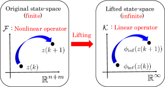
Fig. 1: Nonlinear operator $\mathcal{F}$ on state space and Koopman operator $\mathcal{K}$ on lifted state space

2.1.2 Approximation of Koopman Operator

Since the Koopman operator is the infinite-dimensional operator, it is difficult to be handled in numerical calculations. In this subsection, we give the finite-dimensional approximation of the Koopman operator. To this end, we define the $N_{\phi}$-dimensional lifting function $\phi(z):\mathbb{R}^{n+m}\to\mathbb{R}^{N_{\phi}}$ as

$$\phi(z)=\left[\begin{array}[]{c}\phi_{1}(z)\\ \vdots\\ \phi_{N_{\phi}}(z)\end{array}\right]\in\mathbb{R}^{N_{\phi}}.$$ (19)

Furthermore, we let $\mathcal{A}\in\mathbb{R}^{N_{\phi}\times N_{\phi}}$ be a finite-dimensional matrix that approximates the Koopman operator $\mathcal{K}$, i.e., the error

$$\|\mathcal{A}\phi(z)-\phi(\mathcal{F}(z))\|$$ (20)

is sufficiently small. With this $\mathcal{A}$, we have the expression

$$\phi(z(k+1))\approx\mathcal{A}\phi(z(k)),$$ (21)

which approximately describes the behavior of $\phi_{\mathrm{inf}}(z)$, defined by (15).

In this paper we propose the method of the data-driven approximation of ${\mathcal{K}}$, i.e., the learning method of ${\mathcal{A}}$ by using some data. In the method, we aim at constructing the model (21) that is compatible with controller design. It is tractable for controller design and its implementation that the model is linear to the input $u$. To this end, we further specialize the class of the lifting function $\phi(z)$ in the following form

$$\phi(z)=\left[\begin{array}[]{c}\psi(x)\\ u\end{array}\right]\in\mathbb{R}^{N+m},$$ (24)

where $\psi(x):\mathbb{R}^{n}\to\mathbb{R}^{N}$ is $N$-dimensional lifting function given by

$$\psi(x)=\left[\begin{array}[]{c}\psi_{1}(x)\\ \vdots\\ \psi_{N}(x)\end{array}\right]\in\mathbb{R}^{N},$$ (28)

and $N+m=N_{\phi}$ holds. Let the matrix $\mathcal{A}$ be partitioned as

$$\mathcal{A}=\left[\begin{array}[]{cc}A&B\\ &*\end{array}\right]\in\mathbb{R}^{(N+m)\times(N+m)},$$ (31)

where $A\in\mathbb{R}^{N\times N}$ and $B\in\mathbb{R}^{N\times m}$. Then, it follows from (21) that the following expression of the time-evolution of $\psi(x)$ holds.

$$\psi(x(k+1))\approx A\psi(x(k))+Bu(k).$$

In addition, we give the approximation of the output equation in (3) by

$$y(k)\approx C\psi(x(k)),$$

where $C\in\mathbb{R}^{l\times N}$. For simplicity of notation, we let $\psi(k)=\psi(x(k))$. Then, we obtain the state-space model defined on the functional space as

$$\left\{\begin{array}[]{ll}\psi(k+1)&=A\psi(k)+Bu(k),\\ y(k)&=C\psi(k).\end{array}\right.$$ (34)

The model (34) approximately describes the nonlinear input-output behavior generated by (3). In this paper, the model (34) is called the “Koopman model”. The aim of this paper is to propose the learning method of the system matrices $\left(A,B,C\right)$ based on some data-sets.

2.1.3 Learning Koopman Operator

For simplicity of notation, we define the following data-matrices based on the sequences of the input, output, and state of the system (3).

$$U_{k} :=\left[u(k)~{}u(k+1)~{}\cdots~{}u(k+M-1)\right]\in\mathbb{R}^{m\times M},$$

$$Y_{k} :=\left[y(k)~{}y(k+1)~{}\cdots~{}y(k+M-1)\right]\in\mathbb{R}^{m\times M},$$

$$\Psi_{k} :=\left[\psi(k)~{}\psi(k+1)~{}\cdots~{}\psi(k+M-1)\right]\in\mathbb{R}^{N\times M},$$

$$\Psi_{k+1} :=\left[\psi(k+1)~{}\psi(k+2)~{}\cdots~{}\psi(k+M)\right]\in\mathbb{R}^{N\times M}.$$

It should be noted that $\Psi_{k}$ and $\Psi_{k+1}$ are constructed by using the measured data on the state, $\{x(k),\ldots,x(k+M)\}$. In this paper, it is assumed that the data-set $\left(U_{k},Y_{k},\Psi_{k},\Psi_{k+1}\right)$ is given and available for learning the Koopman operator that expresses (3). The problem of learning is formulated as follows.

Given the data-matrices $(U_{k},Y_{k},\Psi_{k},\Psi_{k+1})$, solve the optimization problem:

$$\min_{A,B,C} \quad J_{1}(A,B)+J_{2}(C),$$ (35)

where $J_{1}(A,B)$ and $J_{2}(C)$ are given by

$$J_{1}(A,B) :=\left\|\Psi_{k+1}-\left[A~{}B\right]\left[\begin{array}[]{c}\Psi_{k}\\ U_{k}\end{array}\right]\right\|_{F}^{2},$$ (38)

$$J_{2}(C) :=\left\|Y_{k}-C\Psi_{k}\right\|_{F}^{2}.$$ (39)

The solution to the optimization problem (35) provides the system matrices $(A^{\dagger},B^{\dagger},C^{\dagger})$ of the Koopman model (34). It is assumed that $\left[\Psi_{k}^{\top}U_{k}^{\top}\right]^{\top}$ is of full row rank, which is a natural assumption when rich data is available for learning. Then, the learned matrices $(A^{\dagger},B^{\dagger},C^{\dagger})$ are uniquely determined by any given data.

Remark 1

Note that the optimization problem (35) is separately solvable: the minimization of just $J_{1}(A,B)$ provides the optimal $(A^{\dagger},B^{\dagger})$, while that of $J_{2}(C)$ provides the optimal $C^{\dagger}$.

2.2 Dissipativity

In this subsection, we review dissipativity of dynamical systems. Dissipativity is a property of characterizing dynamical systems and plays an important role in system analysis, in particular, the analysis of feedback or more general interconnection of dynamical systems (see e.g., the pioneering work by Willems (1972) and developments e.g., by Hill and Moylan (1976, 1977)). Dissipativity is defined for the input-output system (3) as follows.

Definition 1

Given a scalar function $s(u,y):\mathbb{R}^{m+l}\to\mathbb{R}$, the system (3) is said to be dissipative for $s(u,y)$ if there is a non-negative function $V(x):\mathbb{R}^{n}\to\mathbb{R}_{+}$ such that the inequality

$$V(x(k))-V(x(0))\leq\sum_{\tau=0}^{k}s(u(\tau),y(\tau)),\quad\forall k\geq 0$$ (40)

holds.

The functions $s(u,y)$ and $V(x)$ and the inequality (40) are called the supply rate, storage function, and dissipation inequality, respectively. In the view of dissipativity theory, dynamical systems are briefly modeled by an one-dimensional difference inequality (40), instead of a multi-dimensional difference equation (3).

A characterization of dissipative linear dynamical systems is given. We specialize the supply rate $s(u,y)$ in the quadratic form as

$$s(u,y)=-\left[\begin{array}[]{c}y\\ u\end{array}\right]^{\mathrm{T}}\Xi\left[\begin{array}[]{c}y\\ u\end{array}\right],$$ (45)

where $\Xi$ is the real symmetric matrix of

$$\Xi=\left[\begin{array}[]{cc}\Xi_{11}&\Xi_{12}\\ \Xi_{12}^{\mathrm{T}}&\Xi_{22}\end{array}\right].$$ (48)

Even for the specialization of the supply rate, the dissipativity includes some important property of dynamical systems. For example, the dissipativity with respect to $(\Xi_{11},\Xi_{12},\Xi_{22})=(0,-1,0)$ represents the passivity of dynamical systems, and that with respect to $(\Xi_{11},\Xi_{12},\Xi_{22})=(1,0,-\gamma)$ for some positive constant $\gamma$ represents the bounded $L_{2}$ gain.

The dissipativity of linear input-output systems, e.g., described by (34), is characterized by the following lemma.

Lemma 1

The following statements (i) and (ii) are equivalent (see the book by Brogliato et al. (2007)).

(i)

The Koopman model (34) is dissipative for the supply rate $s(u,y)$ of (45).

(ii)

There exists a symmetric matrix $P$ such that the following inequalities hold.

$$P\succ 0$$ (49)

$$\left[\begin{array}[]{cc}A&B\\ I&0\end{array}\right]^{\mathrm{T}}\left[\begin{array}[]{cc}P&0\\ 0&-P\end{array}\right]\left[\begin{array}[]{cc}A&B\\ I&0\end{array}\right]+\Theta\prec 0,$$ (56)

where

$$\Theta=\left[\begin{array}[]{cc}C&0\\ 0&I\end{array}\right]^{\mathrm{T}}\Xi\left[\begin{array}[]{cc}C&0\\ 0&I\end{array}\right].$$

3 Learning Koopman Operator with Dissipativity-Constraints

In this section, we propose a learning method of nonlinear dynamical systems with incorporating a priori information on the system dissipativity. We assume that the supply rate $s(u,y)$ characterizing the system dissipativity is already given and available for learning. Then, we aim at incorporating the dissipativity information into the Koopman model (34).

3.1 Problem Setting

We aim at constructing the Koopman model (34) that satisfies the dissipation inequality (40) based on some data-sets. This learning problem of the system matrices $\left(A,B,C\right)$ of (34) is reduced to the problem of (35) subject to the dissipativity constraints (49) and (56). The problem is mathematically formulated as follows.

Problem 3.1

Given the real symmetric matrix $\Xi$ and the data-matrices $\left(U_{k},Y_{k},\Psi_{k},\Psi_{k+1}\right)$, solve the optimization problem:

$$\min_{P,A,B,C} \quad{J_{1}(A,B)}+J_{2}(C)$$

sub to $$\quad(\ref{eq.b3_1}),(\ref{eq.b3}).$$

Suppose that the optimal solution to Problem 3.1 is given by $(P^{*},A^{*},B^{*},C^{*})$. Then the Koopman model (34) with $(A^{*},B^{*},C^{*})$ is dissipative for the supply rate $s(u,y)$ of (45).

Note that the dissipativity constraint, described by (49) and (56), is non-convex in decision variables $\left(P,A,B,C\right)$. It is not numerically tractable to solve Problem 3.1. In the next subsection, we try to approximately reduce the problem to a convex one.

3.2 Convex Approximation of Problem 3.1

On the basis of the variable transformation technique by Hoagg et al. (2004); Abe et al. (2016), the nonlinear inequality (56) is reduced into a linear matrix one. First, we expand the inequality (56) as

$$\left[\begin{array}[]{cc}P-C^{\mathrm{T}}\Xi_{11}C&-C^{\mathrm{T}}\Xi_{12}\\ -\Xi_{12}^{\mathrm{T}}C&-\Xi_{22}\end{array}\right]-\left[A~{}B\right]^{\mathrm{T}}P\left[A~{}B\right]\succ 0.$$ (59)

Noting $P\succ 0$ and applying the Schur complement to (59), it follows that

$$\left[\begin{array}[]{cc}\left[\begin{array}[]{cc}P-C^{\mathrm{T}}\Xi_{11}C&-C^{\mathrm{T}}\Xi_{12}\\ -\Xi_{12}^{\mathrm{T}}C&-\Xi_{22}\end{array}\right]&\left[\begin{array}[]{c}A^{\mathrm{T}}P\\ B^{\mathrm{T}}P\end{array}\right]\\ \left[PA~{}PB\right]&P\end{array}\right]\succ 0$$ (66)

holds.

Next, we apply the variable transformation to $(P,A,B)$. We let

$$R=PA,\quad S=PB$$ (67)

to reduce (66) to the inequality

$$\left[\begin{array}[]{ccc}P-C^{\mathrm{T}}\Xi_{11}C&-C^{\mathrm{T}}\Xi_{12}&R^{\mathrm{T}}\\ -\Xi_{12}^{\mathrm{T}}C&-\Xi_{22}&S^{\mathrm{T}}\\ R&S&P\end{array}\right]\succ 0.$$ (71)

Note that this (71) is still equivalent to (56). This is because that the solution $(P,R,S,C)$ to (71) generates the solution to (56) by $(P,A,B,C)=(P,P^{-1}R,P^{-1}S,C)$.

Now, suppose that $C$ is given, e.g., by just minimizing $J_{2}(C)$ based on the data-set $(Y_{k},\Phi_{k})$. Then, the inequality (71) is linear in the matrices $(P,R,S)$, which is numerically tractable.

There is the drawback in the variable transformation of (67): the cost function $J_{1}(A,B)$ of (38) becomes non-convex in the transformed variables $(P,R,S)$, which is numerically intractable. To overcome the drawback and to numerically obtain the feasible solution to Problem 3.1, we approximately transform $J_{1}(A,B)$ to a convex one. To this end, we introduce $W=P$, as a weighting matrix, into $J_{1}(A,B)$ to define a new cost function as follows.

$$J_{1,W}(P,R,S) =\left\|W\left(\Psi_{k+1}-\left[A~{}B\right]\left[\begin{array}[]{c}\Psi_{k}\\ U_{k}\end{array}\right]\right)\right\|_{F}^{2}$$ (74)

$$=\left\|P\Psi_{k+1}-\left[R~{}S\right]\left[\begin{array}[]{c}\Psi_{k}\\ U_{k}\end{array}\right]\right\|_{F}^{2}.$$ (77)

The function $J_{1,W}(P,R,S)$ of (77) is convex in the matrices $(P,R,S)$. The minimization problem of $J_{1,W}(P,R,S)$ under the inequalities (49) and (71) is in the class of the convex optimization. The optimization problem is summarized as follows.

Problem 3.2

Given the system matrix $C$, the real symmetric matrix $\Xi$, and the data-matrices $\left(U_{k},\Psi_{k},\Psi_{k+1}\right)$, solve the optimization problem:

$$\min_{P,R,S} \quad{J_{1,W}(P,R,S)}$$

$$\mathrm{sub\ to} \quad(\ref{eq.b3_1}),(\ref{eq.b11}).$$

Suppose that Problem 3.2 is feasible and that the solution $(\hat{P},\hat{R},\hat{S})$ is given. Then, we obtain the system matrices as

$$\hat{A}=\hat{P}^{-1}\hat{R},\quad\hat{B}=\hat{P}^{-1}\hat{S}.$$ (78)

We have the following proposition for the constructed model based on the solution to Problem 3.2.

Proposition 2

Suppose that Problem 3.2 is feasible and that system matrices are given by (78). Then, the quadruplet $(\hat{P},\hat{A},\hat{B},C)$ is the feasible solution to Problem 3.1. In other words, the Koopman model (34) with $(\hat{A},\hat{B},C)$ is dissipative for the supply rate $s(u,y)$ of (45).

As implied in the proposition, the solution to Problem 3.2 is the feasible solution, but may not be the optimal solution to Problem 3.1. In general, the solution $(\hat{P},\hat{A},\hat{B},C)$ is conservative for Problem 3.1. In the following subsection, we aim at finding a better approximation of Problem 3.1.

3.3 Sequential Convex Approximation of Problem 3.1

In this subsection, we give the efficient solution method for Problem 3.1 based on the overbounding method proposed by Sebe (2018). In the overbounding method, the inner approximations of nonlinear matrix inequalities are sequentially constructed. This sequential method contributes to gradually reduce the conservativeness of the solution of Problem 3.2.

Suppose that Problem 3.2 is feasible and that the feasible solution to Problem 3.1, denoted by $(\hat{P},\hat{A},\hat{B})$, is constructed. Then, we try to update the initial guess $(\hat{P},\hat{A},\hat{B})$ to reduce the conservativeness, i.e., to further reduce $J_{1}(A,B)$. First, we transform the decision variables of Problem 3.1, denoted by $(P,A,B)$, into $(\Delta P,\Delta A,\Delta B)$ as follows.

$$P=\hat{P}+\Delta P,\quad A=\hat{A}+\Delta A,\quad B=\hat{B}+\Delta B.$$

Further, we let $G$ and $H$ be additional decision variables. With those $G$ and $H$, we define the inequality condition described in (85), where $Q(\Delta P,\Delta A,\Delta B)$ is given by (95) and $F(\Delta P)$ is given by

$$\mathrm{He}\left(\left[\begin{array}[]{ccc}Q(\Delta P,\Delta A,\Delta B)&\left[\begin{array}[]{c}0\\ \Delta P\end{array}\right]&0\\ 0&-G&G\\ -H\left[\begin{array}[]{ccc}\Delta A&\Delta B&0\end{array}\right]&0&-H\end{array}\right]\right)\prec 0.$$ (85)

$$Q(\Delta P,\Delta A,\Delta B) =-\cfrac{1}{2}\left[\begin{array}[]{cc}-F(\Delta P)&0\\ 0&\hat{P}+\Delta P\end{array}\right]+\left[\begin{array}[]{ccc}0&0&0\\ -\hat{P}\hat{A}&-\hat{P}\hat{B}&0\end{array}\right]$$ (90)

$$\hskip 14.22636pt+\left[\begin{array}[]{ccc}0&0&0\\ -\Delta P\hat{A}&-\Delta P\hat{B}&0\end{array}\right]+\left[\begin{array}[]{ccc}0&0&0\\ -\hat{P}\Delta A&-\hat{P}\Delta B&0\end{array}\right].$$ (95)

$$F(\Delta P)=\left[\begin{array}[]{cc}\hat{P}+\Delta P-C^{\mathrm{T}}\Xi_{11}C&-C^{\mathrm{T}}\Xi_{12}\\ -\Xi_{12}^{\mathrm{T}}C&-\Xi_{22}\end{array}\right].$$

We show that (85) is a sufficient condition for (56) as stated in the following proposition.

Proposition 3

Suppose (85) holds. Then, letting $(P,A,B)=(\hat{P}+\Delta P,\hat{A}+\Delta A,\hat{B}+\Delta B)$, it holds that (56).

The proof follows Proposition 3 in the work by Sebe (2018) and is omitted in this paper. Furthermore, it should be noted that (85) is linear in $(\Delta P,\Delta A,\Delta B,G)$. This implies that for any fixed $H$, (85) is in the form of LMIs and is numerically tractable.

Recall $J_{1}(A,B)$ of $(\ref{eq.b1})$ to obtain the expression

$$J_{1}(\hat{A}+\Delta A,\hat{B}+\Delta B)$$

$$=\left\|\Psi_{k+1}-\left[\hat{A}+\Delta A,~{}\hat{B}+\Delta B\right]\left[\begin{array}[]{c}\Psi_{k}\\ U_{k}\end{array}\right]\right\|_{F}^{2}.$$ (98)

Then, the problem of finding $(\Delta P,\Delta A,\Delta B,G)$ that minimizes $J_{1}(\hat{A}+\Delta A,\hat{B}+\Delta B)$ under the constraint (85) based on the initial guess $(\hat{P},\hat{A},\hat{B})$ is stated as follows

Problem 3.3

Given the system matrix $C$, the real symmetric matrix $\Xi$, the data-matrices $\left(U_{k},\Psi_{k},\Psi_{k+1}\right)$, the feasible solution to Problem 3.1, denoted by $(\hat{P},\hat{A},\hat{B})$, and the real matrix $H$, solve the optimization problem:

$$\min_{\Delta P,\Delta A,\Delta B,G} \quad J_{1}(\hat{A}+\Delta A,\hat{B}+\Delta B)$$

$$\mathrm{sub\ to} \quad(\ref{eq.c8}),~{}\hat{P}+\Delta P\succ 0.$$

With the optimal solution $(\Delta\bar{P},\Delta\bar{A},\Delta\bar{B})$ to Problem 3.3, we obtain the matrices

$$\bar{P}=\hat{P}+\Delta\bar{P},\quad\bar{A}=\hat{A}+\Delta\bar{A},\quad\bar{B}=\hat{B}+\Delta\bar{B}.$$

The notation on the optimal solutions to Problems 3.1–3.3 are summarized on Table 1.

Table 1: Notation of optimal solutions

Problem	Solution
Unconstrained (35)	$(A^{\dagger},B^{\dagger},C^{\dagger})$
Problem 3.1	$(P^{*},A^{*},B^{*},C^{*})$
Problem 3.2	$(\hat{P},\hat{R},\hat{S})\to(\hat{P},\hat{A},\hat{B})$
Problem 3.3	$(\Delta\bar{P},\Delta\bar{A},\Delta\bar{B})\to(\bar{P},\bar{A},\bar{B})$

Note that the solution $(\bar{P},\bar{A},\bar{B})$ is the less conservative solution to Problem 3.1 than the initial guess $(\hat{P},\hat{A},\hat{B})$ for any real matrix $H$ satisfying

$$H+H^{\mathrm{T}}\succ 0.$$ (99)

This fact is mathematically stated in the following proposition.

Proposition 4

Suppose that Problem 3.2 is feasible. Then, for any real matrix $H$ satisfying the condition (99), Problem 3.3 is feasible. In addition, if $(\hat{P},\hat{A},\hat{B})$ is not the solution to Problem 3.1, the strict inequality

$$J_{1}(\bar{A},\bar{B})<J_{1}(\hat{A},\hat{B})$$ (100)

holds.

Proof. First, we prove that Problem 3.3 has at least one feasible solution $(\Delta P,\Delta A,\Delta B,G)=(\Delta P_{f},\Delta A_{f},\Delta B_{f},G_{f})$. Let $(\Delta P_{f},\Delta A_{f},\Delta B_{f})=\left(0,0,0\right)$. Then, the left hand side of (85) is reduced to

$$\mathrm{He}\left(\left[\begin{array}[]{cc}Q(0,0,0)&0\\ 0&X\end{array}\right]\right),$$ (103)

where

$$Q(0,0,0) =-\frac{1}{2}\left[\begin{array}[]{cc}\left[\begin{array}[]{cc}\hat{P}-C^{\mathrm{T}}\Xi_{11}C&-C^{\mathrm{T}}\Xi_{12}\\ -\Xi_{12}^{\mathrm{T}}C&-\Xi_{22}\end{array}\right]&\left[\begin{array}[]{c}\hat{A}^{\mathrm{T}}\hat{P}\\ \hat{B}^{\mathrm{T}}\hat{P}\end{array}\right]\\ \left[\hat{P}\hat{A}~{}\hat{P}\hat{B}\right]&\hat{P}\end{array}\right],$$ (110)

$$X =\left[\begin{array}[]{cc}-G&G\\ 0&-H\end{array}\right].$$ (113)

Since $(\hat{P},\hat{A},\hat{B})$ satisfies the inequality (71), we see that

$$\mathrm{He}\left(Q(0,0,0)\right)\prec 0$$ (114)

holds. In addition, letting $G_{f}=\frac{1}{2}\left(H+H^{\mathrm{T}}\right)$, we have

$$\mathrm{He}\left(X\right)=-\left[\begin{array}[]{cc}(H+H^{\mathrm{T}})&-\frac{1}{2}(H+H^{\mathrm{T}})\\ -\frac{1}{2}(H+H^{\mathrm{T}})&(H+H^{\mathrm{T}})\end{array}\right]\prec 0.$$ (117)

It follows from (114) and (117) that

$$(\Delta P_{f},\Delta A_{f},\Delta B_{f},G_{f})=\left(0,0,0,\frac{1}{2}(H+H^{\mathrm{T}})\right)$$ (118)

satisfies the constraint (85) and is the feasible solution to Problem 3.3.

Next, we prove that (100) holds. Since the constraint (85) is the strict inequality, i.e., the feasible region is open, the neighborhood of (118) still gives the feasible solution. In addition, recall that the cost function $J_{1}(\hat{A}+\Delta A,\hat{B}+\Delta B)$ is strongly convex in $(\Delta A,\Delta B)$. Then, $J_{1}(\hat{A}+\Delta A,\hat{B}+\Delta B)$ strictly decreases for some point in the neighborhood compared with $J_{1}(\hat{A}+\Delta A_{f},\hat{B}+\Delta B_{f})$. This completes the proof of the proposition. $\Box$

On the basis of the fact stated in Proposition 4, a sequential algorithm of solving Problem 3.1 is proposed. Suppose that Problem 3.3 with $(\hat{P},\hat{A},\hat{B},H)=(\bar{P}_{i},\bar{A}_{i},\bar{B}_{i},H_{i})$ has the optimal solution $(\Delta\bar{P}_{i},\Delta\bar{A}_{i},\Delta\bar{B}_{i},\bar{G}_{i})$. Consider the updating law

$$(\bar{P}_{i+1},\bar{A}_{i+1},\bar{B}_{i+1},H_{i+1})$$

$$\leftarrow(\bar{P}_{i}+\Delta\bar{P}_{i},\bar{A}_{i}+\Delta\bar{A}_{i},\bar{B}_{i}+\Delta\bar{B}_{i},\bar{G}_{i}).$$ (119)

Then, by sequentially solving Problem 3.3 with the updated $(\hat{P},\hat{A},\hat{B},H)=(\bar{P}_{i+1},\bar{A}_{i+1},\bar{B}_{i+1},H_{i+1})$, we obtain the solution $(\Delta\bar{P}_{i+1},\Delta\bar{A}_{i+1},\Delta\bar{B}_{i+1},\bar{G}_{i+1})$, which generates the less conservative solution to Problem 3.1.

We propose to sequentially solve Problem 3.3 with updated $(\bar{P}_{i+1},\bar{A}_{i+1},\bar{B}_{i+1},H_{i+1})$ to obtain the less conservative solution to Problem 3.1. The sequential solution method is summarized in Algorithm.

[l]Algorithm

• Find the solution $(\hat{P},\hat{R},\hat{S})=(\hat{P}_{0},\hat{R}_{0},\hat{S}_{0})$ to Problem 3.2 and obtain $\bar{A}_{0}=\hat{P}_{0}^{-1}\hat{R}_{0}$ and $\bar{B}_{0}=\hat{P}_{0}^{-1}\hat{S}_{0}$. In addition, let $H_{0}=I$ and $i=0$.

• Given $(\hat{P},\hat{A},\hat{B},H)=(\bar{P}_{i},\bar{A}_{i},\bar{B}_{i},H_{i})$, find the solution $(\Delta\bar{P}_{i},\Delta\bar{A}_{i},\Delta\bar{B}_{i},\bar{G}_{i})$ to Problem 3.3.

• Apply (119) to obtain $(\bar{P}_{i+1},\bar{A}_{i+1},\bar{B}_{i+1},H_{i+1})$. Then, set $i\leftarrow i+1$ and go to Step1.

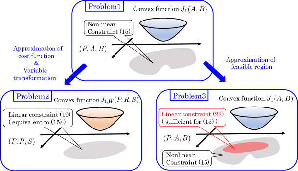
Fig. 2: Cost functions and feasible regions of Problems 3.1–3.3

Finally, the relationship among Problems 3.1–3.3 is illustrated in Fig. 2. Recall that Problem 3.1 is the minimization problem of the convex cost function $J_{1}$ under the nonlinear matrix inequality (56). The problem is approximated in different two ways as Problems 3.2 and 3.3. In Problem 3.2, $J_{1}$ is distorted and replaced by another convex one $J_{1,W}$, while (56) is equivalently reduced to the LMI (71). In Problem 3.3, the inner convex approximation of (56) is found and utilized, while keeping $J_{1}$. Problem 3.2 is solved aiming at finding the feasible solution to Problem 3.1, while Problem 3.3 is sequentially solved aiming at reducing the conservativeness of the solution.

4 Numerical Experiment

In this section, we demonstrate the procedure of learning a nonlinear dynamical system by applying the proposed algorithm. Consider a continuous-time nonlinear dynamical system described by

$$\left\{\begin{array}[]{lll}\dot{x}_{1}(t)&=x_{2}(t),\\ \dot{x}_{2}(t)&=-2x_{2}(t)+x(1)\cos\left(x_{1}(t)+x_{2}(t)\right)+u(t),\\ y(t)&=x_{2}(t).\end{array}\right.$$ (123)

It is known that the system is dissipative with respect to $(\Xi_{11},\Xi_{12},\Xi_{22})=(0,-1,0)$, i.e., the system is passive (see e.g., the work by Zakeri and Antsaklis (2019)). In this experiment, we aim at accurately learning the dynamical system in the Koopman model (34), while incorporating the passivity property.

In the experimental setup, we consider that the time series of $x(t)$, $u(t)$, and $y(t)$ are sampled at each 0.01 time period from the system (123), which are denoted by $\{x(k)\}$, $\{u(k)\}$, and $\{y(k)\}$, respectively. The input series $\{u(k)\}$ for learning are determined from randomly selected values from the uniform distribution in $[\,-1,\,1\,]$. Then, the state and output series $\{x(k)\}$ and $\{y(k)\}$ are measured synchronously. In total, the data at 5000 samples are obtained.

We try to apply Algorithm to the data $\{x(k)\}$, $\{u(k)\}$, and $\{y(k)\}$. To this end, first, we let $(\Xi_{11},\Xi_{12},\Xi_{22})=(0,-1,-0.2)$ and its corresponding dissipativity constraint be defined to inherit the a priori information on the passivity in a relaxed form. Furthermore, let the lifting function $\psi(x(k))$ be composed of the state $x(k)=[\,x_{1}(k),x_{2}(k)\,]^{\mathrm{T}}$ and thin plate spline radial basis functions $\psi_{i}(x(k))$, $i\in\{1,2,\ldots,8\}$, where $\psi_{i}(x(k))$ is given by

$$\psi_{i}(x(k))=\|x(k)-r_{i}\|_{2}^{2}\ln{\|x(k)-r_{i}\|_{2}}$$

and the values of $r_{i}$ are selected randomly from the uniform distribution on the unit box. Then, the lifting function $\psi(x(k))$ is described by

$$\psi(x(k))=\left[\,x(k)\ \psi_{1}(x(k))\ \cdots\ \psi_{8}(x(k))\,\right]^{\mathrm{T}}\in\mathbb{R}^{2+8}.$$ (124)

By applying Algorithm, we constructed the dissipativity-constrained Koopman model, which approximates the nonlinear system (123) and is called Model 1. In addition, we constructed two different models by using the same time series data: (Model 2) one is the no-constrained Koopman model, which is simply constructed by solving (35), while (Model 3) the other is the dissipativity-constrained linear model, which is based on $\psi(x(k))=x(k)$ and is constructed by applying the learning method proposed by Abe et al. (2016).

First, to show the model accuracy, the three models are compared with the true nonlinear system (123). The result of the frequency response against the sin-wave input is illustrated in Figs. 3 and 4, where the state trajectory of the models is shown. In the figures, the black solid, blue solid, red dashed, and pink dotted lines represent the state of the true system, Model 1 (proposed model), Model 2, and Model 3, respectively. We see from Fig. 3 that Models 1 and 2, i.e., the Koopman models, accurately express the nonlinear behavior generated by (123), while Model 3, i.e., the linear model, is not. The lifting function with the basis (124) contributes to improving the ability of model expression.

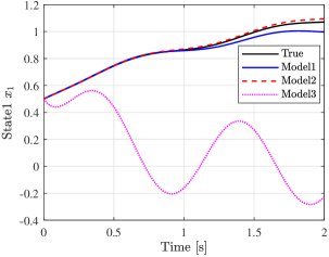
Fig. 3: State trajectory $x_{1}(k)$.

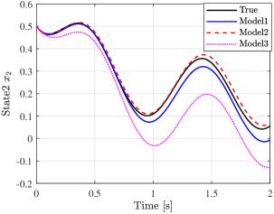
Fig. 4: State trajectory $x_{2}(k)$.

Next, to show the validity of the dissipativity constraint, we define the transfer function for the Koopman model. Letting $G(e^{j\omega T})=C\left(e^{j\omega T}I-A\right)^{-1}B$, we reduce the dissipativity constraint, characterized by $(\Xi_{11},\Xi_{12},\Xi_{22})=(0,-1,-0.2)$, to

$$\mathrm{Re}[G(e^{j\omega T})]\geq-0.1,\quad\forall\omega\in\mathbb{R}.$$

Then, the Nyquist plot of the $G(e^{j\omega T})$ for the three models is illustrated in Fig. 5. As illustrated in the figure, Models 1 and 3 satisfy the dissipativity constraint, while Model 2 violates. This shows that the dissipativity constraint imposed on the learning problems is valid.

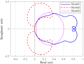
Fig. 5: Comparison of Nyquist plot

5 Conclusion

This paper addressed the learning problem of nonlinear dynamical systems with incorporating the a priori information on the quadratic dissipativity. The problem was reduced to the data-driven approximation of the Koopman operator under the dissipativity constraint, which was called Problem 3.1 in this paper. Then, the solution method to the problem was given and summarized in Algorithm. There are two main contributions of this paper. 1) One is in this numerically efficient algorithm, which sequentially solves LMIs. 2) The other is the performance analysis of the algorithm, which is stated in Proposition 4. In the analysis, it is guaranteed that the Koopman model constructed by the algorithm fits given data more accurately than the model defined at any initial guess.

References

- Abe et al. (2016) Abe, Y., Inoue, M., and Adachi, S. (2016). Subspace identification method incorporated with a priori information characterized in frequency domain. In 2016 European Control Conference (ECC), 1377–1382. IEEE.
- Alenany et al. (2011) Alenany, A., Shang, H., Soliman, M., and Ziedan, I. (2011). Improved subspace identification with prior information using constrained least squares. IET Control Theory & Applications, 5(13), 1568–1576.
- Brogliato et al. (2007) Brogliato, B., Lozano, R., Maschke, B., and Egeland, O. (2007). Dissipative systems analysis and control. Theory and Applications, 2.
- De la Rosa and Yu (2016) De la Rosa, E. and Yu, W. (2016). Randomized algorithms for nonlinear system identification with deep learning modification. Information Sciences, 364, 197–212.
- Goethals et al. (2003) Goethals, I., Van Gestel, T., Suykens, J., Van Dooren, P., and De Moor, B. (2003). Identification of positive real models in subspace identification by using regularization. IEEE Transactions on Automatic Control, 48(10), 1843–1847.
- Hill and Moylan (1976) Hill, D. and Moylan, P. (1976). The stability of nonlinear dissipative systems. IEEE Transactions on Automatic Control, 21(5), 708–711.
- Hill and Moylan (1977) Hill, D.J. and Moylan, P.J. (1977). Stability results for nonlinear feedback systems. Automatica, 13(4), 377–382.
- Hoagg et al. (2004) Hoagg, J.B., Lacy, S.L., Erwin, R.S., and Bernstein, D.S. (2004). First-order-hold sampling of positive real systems and subspace identification of positive real models. In Proceedings of the 2004 American control conference, volume 1, 861–866. IEEE.
- Inoue (2019) Inoue, M. (2019). Subspace identification with moment matching. Automatica, 99, 22–32.
- Jin et al. (2016) Jin, X., Shao, J., Zhang, X., An, W., and Malekian, R. (2016). Modeling of nonlinear system based on deep learning framework. Nonlinear Dynamics, 84(3), 1327–1340.
- Kevrekidis et al. (2015) Kevrekidis, I., Rowley, C., and Williams, M. (2015). A kernel-based method for data-driven Koopman spectral analysis. Journal of Computational Dynamics, 2(2), 247–265.
- Koopman (1931) Koopman, B.O. (1931). Hamiltonian systems and transformation in hilbert space. Proceedings of the National Academy of Sciences of the United States of America, 17(5), 315–318.
- Korda and Mezić (2018) Korda, M. and Mezić, I. (2018). Linear predictors for nonlinear dynamical systems: Koopman operator meets model predictive control. Automatica, 93, 149–160.
- Lacy and Bernstein (2003) Lacy, S.L. and Bernstein, D.S. (2003). Subspace identification with guaranteed stability using constrained optimization. IEEE Transactions on automatic control, 48(7), 1259–1263.
- Miller and De Callafon (2013) Miller, D.N. and De Callafon, R.A. (2013). Subspace identification with eigenvalue constraints. Automatica, 49(8), 2468–2473.
- Okada and Sugie (1996) Okada, M. and Sugie, T. (1996). Subspace system identification considering both noise attenuation and use of prior knowledge. In Proceedings of 35th IEEE Conference on Decision and Control, volume 4, 3662–3667. IEEE.
- Sebe (2018) Sebe, N. (2018). Sequential convex overbounding approximation method for bilinear matrix inequality problems. IFAC-PapersOnLine, 51(25), 102–109.
- Sitompul (2013) Sitompul, E. (2013). Adaptive neural networks for nonlinear dynamic systems identification. In 2013 Fifth International Conference on Computational Intelligence, Modelling and Simulation, 8–13. IEEE.
- Willems (1972) Willems, J.C. (1972). Dissipative dynamical systems part i: General theory. Archive for Rational Mechanics and Analysis, 45(5), 321–351. 10.1007/BF00276493.
- Williams et al. (2015) Williams, M.O., Kevrekidis, I.G., and Rowley, C.W. (2015). A data–driven approximation of the Koopman operator: Extending dynamic mode decomposition. Journal of Nonlinear Science, 25(6), 1307–1346.
- Yoshimura et al. (2019) Yoshimura, S., Matsubayashi, A., and Inoue, M. (2019). System identification method inheriting steady-state characteristics of existing model. International Journal of Control, 92(11), 2701–2711.
- Zakeri and Antsaklis (2019) Zakeri, H. and Antsaklis, P.J. (2019). Passivity and passivity indices of nonlinear systems under operational limitations using approximations. International Journal of Control, (just-accepted), 1–20.