Sequential Recommendation with Dual Side
Neighbor-based Collaborative Relation Modeling

Abstract.

Sequential recommendation task aims to predict user preference over items in the future given user historical behaviors. The order of user behaviors implies that there are resourceful sequential patterns embedded in the behavior history which reveal the underlying dynamics of user interests. Various sequential recommendation methods are proposed to model the dynamic user behaviors. However, most of the models only consider the user’s own behaviors and dynamics, while ignoring the collaborative relations among users and items, i.e., similar tastes of users or analogous properties of items. Without modeling collaborative relations, those methods suffer from the lack of recommendation diversity and thus may have worse performance. Worse still, most existing methods only consider the user-side sequence and ignore the temporal dynamics on the item side. To tackle the problems of the current sequential recommendation models, we propose Sequential Collaborative Recommender (SCoRe) which effectively mines high-order collaborative information using cross-neighbor relation modeling and, additionally utilizes both user-side and item-side historical sequences to better capture user and item dynamics. Experiments on three real-world yet large-scale datasets demonstrate the superiority of the proposed model over strong baselines.

ACM Reference Format:
Jiarui Qin, Kan Ren, Yuchen Fang, Weinan Zhang, Yong Yu. 2020. Sequential Recommendation with Dual Side Neighbor-based Collaborative Relation Modeling. In Proceedings of the 13th ACM International Conference on Web Search and Data Mining (WSDM ’20), February 3-7, 2020, Houston, TX, USA. ACM, New York, NY, USA, 9 pages. https://doi.org/10.1145/3336191.3371842

1. Introduction

With the emergence of large online information systems such as e-commerce platform, the amount of user behavioral data grows rapidly. Therefore, in recent years, the researchers in both academic and industrial fields have devoted many efforts on sequential recommendation task which aims to mine the resourceful yet complex temporal dynamics embedded in user behavior sequences.

As has been stated in many related works (Hidasi and Karatzoglou, 2018; Koren, 2009; He et al., 2016; Agarwal et al., 2009), the temporal dynamics have high impacts on the future user behaviors, especially accounted for concept drifting (Widmer and Kubat, 1996), long-term behavior dependency (Koren, 2009), periodic patterns (Ren et al., 2018a), etc.

Commonly, the current sequential recommendation models regard user’s purchasing or browsing behaviors as “token”s in the natural language processing (NLP) field. And the mainstream models use sequential modeling techniques that are widely used in NLP such as recurrent neural networks (RNNs) (Hidasi et al., 2016; Zhou et al., 2018a), convolutional neural networks (CNNs) (Tang and Wang, 2018) and Transformer (Kang and McAuley, 2018). These models make huge success on sequential recommendation task with many deployed real-world applications (Zhou et al., 2018a; Wu et al., 2016).

Despite the success of current sequential recommendation methods, there are still some limitations of them. The first one is that most of the models (Hidasi et al., 2016; Tang and Wang, 2018; Kang and McAuley, 2018) only consider user’s (or item’s) own interaction history, while ignoring similar users or items that have collaborative relations with itself. Therefore, each user (item) only know her (its) own behaviors, it is bad for the variety of recommendation and may hurt the recommendation performance.

We could regard the user-item interactions as a bipartite graph in which the nodes are users and items, and links are interaction records as illustrated in Figure 1. Traditional models (Koren, 2009, 2008) only consider the directly interacted items (users) of the target user (item) which are the 1-hop neighbors of the target node. In this way, it is difficult to capture the collaborative relations among users and items. But when we make a step forward and consider the 2-hop neighbors, we find that the neighbors in 2-hop have collaborative relations with the target node because both the 2-hop neighbors and the target node have interacted with the same group of nodes which are the 1-hop neighbors. As these relations are found through 2-hops on the graph, we call them high-order collaborative relations.

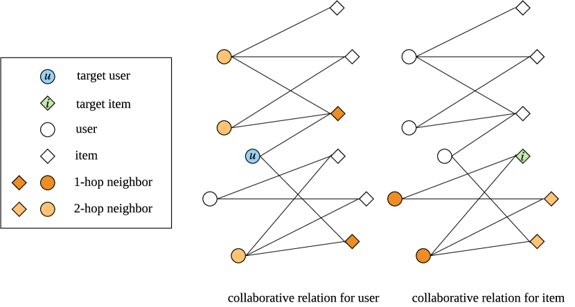
Figure 1. Graph illustration of user-item interactions.

By this means, we may find the corresponding collaborative information for the target user or item. Moreover, there are various patterns across the neighbors that can be utilized. By aggregating these collaborative relations to the representation of users and items, we could model more complex and various user interests (item attractions). And the collaborative modeling can be done in a sequential way to better handle the temporal dynamics.

Another key limitation of current models is that they only consider the user-side temporal dynamics while ignoring the ones on the item side. The user-side sequence consists of the items that are browsed by the user, and thus it could reveal the user’s drifting interests. However, the item-side also contains sequential patterns: an item attracts different users at different time which could reveal the item dynamics such as popularity trend or social topic drift. For example, the recommender system may present Christmas card to a user when the holiday is coming even before her interacting with any related items because the Christmas card has attracted the other users who share similar interests or collaborative relations to that specific user. The modeling of item-side sequence is similar with information dissemination (Petrovic et al., 2011; Rizoiu et al., 2018), which means the item information disseminates from users to users at different time and to predict which user will be the next one that the information disseminates to.

There are already some sequential recommendation models that have tried combining user-side and item-side sequences to perform dual sequence modeling (Wu et al., 2017, 2019a). However, these works intend to consider the two sequences in a relatively independent manner and the sequential representations of both sequences have interactions only in the final prediction stage. Nevertheless, our work aims to model the dual sequences in a more interactive way which means the information of both sequences have interactions along the timeline. As we do collaborative relation capturing from both user-side and item-side, it is natural that we interact both sequences at synchronized time which is illustrated in Figure 2.

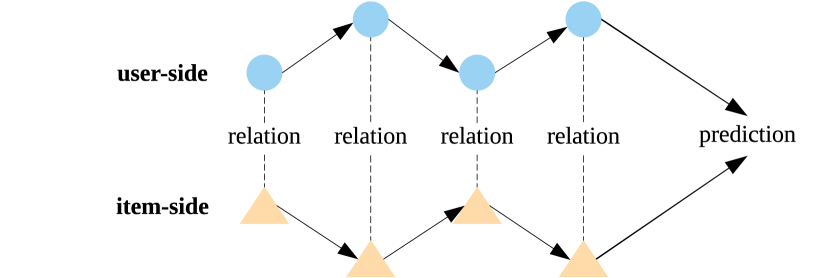
Figure 2. Illustration of interactive dual sequence modeling.

To address the limitations mentioned above, we propose Sequential Collaborative Recommender (SCoRe) which considers high-order collaborative relations and models dual sequences in an interactive and more expressive manner. The contribution of the paper can be summarized in three-fold:

• We propose to aggregate high-order collaborative relations which could enrich the representation of users and items. More importantly, through cross neighbor relation modeling, our model can effectively capture the various and complex patterns in the neighbor-to-neighbor collaborative relations.

• We propose to model both user-side and item-side sequence. Dual sequences interactions are modeled in a more thorough way, which makes the modeling of the dual sequence more expressive.

• We conduct extensive experiments of evaluating and comparing our model with several strong baselines over three real-world yet large-scale recommendation datasets. The results have proved the efficacy of SCoRe model and the detailed analysis reveals some key principles of training our model.

The rest of the paper is organized as follows. Section 2 and Section 3 present the preliminaries and describe the SCoRe model in detail. We also make some discussions about the model efficiency. We conduct comprehensive experiments and present the experimental setups with the corresponding results in Section 4. In Section 5, we discuss about some related works. Finally we conclude the paper and point out some future works in Section 6.

2. Preliminaries

In a recommender system, there are $M$ users in $\mathcal{U}=\{u_{1},\ldots,u_{M}\}$ and $N$ items in $\mathcal{V}=\{v_{1},\ldots,v_{N}\}$. In the history, any user may reveal interests on some items and the interaction behaviors would be tracked in the system as $\mathcal{Y}=\{y_{uv}|u\in\mathcal{U},v\in\mathcal{V}\}$ and

(1) $$y_{uv}=\left\{\begin{array}[]{rcl}1,&&u~{}\text{has interacted with}~{}v;\\ 0,&&\text{otherwise.}\\ \end{array}\right.$$

The user preference $y$ is either implicit feedback (Agarwal et al., 2009), e.g., clicks, or explicit user rating (Koren, 2009). Without loss of generality, we focus on the implicit feedback which is more common in practice. For sequential recommendation, each user-item interaction has the corresponding timestamp $ts$, thus we use the triplet $(u,v,ts)$ to denote one interaction. All the observed interaction records are denote as $\mathcal{T}=\{u,v,ts\}$.

2.1. Interaction Relations

For a target pair of $(u,v)$ that we need to predict the interaction probability, we could extract some interaction relations of the target user $u$ and target item $v$.

Definition 1. (Interaction Set): Given the target user $u$, we can conduct the interaction set of $u$ as

(2) $$\bm{G}(u)=\{v_{j}|y_{uv_{j}}=1\}.$$

The user’s interaction set is the collection of all the items that the user has interacted with. Symmetrically, we can define the item $v$’s interaction set as,

(3) $$\bm{G}(v)=\{u_{i}|y_{u_{i}v}=1\}.$$

which contains all the users that have interaction with the item $v$.

Definition 2. (Co-Interaction Set): To explicitly capture the collaborative relations among users and items, i.e., similar users or similar items, it is natural to consider the users (items) that have similar tastes (attractions). Therefore we define the co-interaction set of $u$ and $v$ respectively as

(4) $$\bm{G}(v|u)=\{u_{i}|y_{{u_{i}}{v_{j}}}=1,v_{j}\in\bm{G}(u)\},\\$$

(5) $$\bm{G}(u|v)=\{v_{j}|y_{{u_{i}}{v_{j}}}=1,u_{i}\in\bm{G}(v)\}.$$

For user $u$, the co-interaction set $\bm{G}(v|u)$ actually consists of a group of users that shares similar behaviors with $u$, because they all interacted with the items in $u$’s interaction set. Therefore they have collaborative relations in some extent. For item $v$, similarly, the co-interaction set $\bm{G}(u|v)$ consists of the items that attract the same group of users ($v$’s interaction set) with the target item $v$.

As shown in Figure 1, we can tell that the interaction set and co-interaction set are essentially the 1-hop and 2-hop neighbors of the rooted node ($u$ or $v$) respectively.

2.2. Evolving Time-sliced Interaction Relations

Now that we have defined the local interaction relations of the user $u$ (item $v$), we take one step forward and consider it in a temporal way.

Specifically, the users (items) may conduct different interactions with different items (users) at different time. Thus, the interaction relations are evolving all the time and could be regarded as a series of time-sliced processes.

To better model the temporal patterns of the interaction relations, we slice the whole timeline into $T$ time frames, each of which is constructed within a unified time interval $\Delta T$. In this way, all observed interactions $\mathcal{T}=\bigcup_{t=1}^{T}\mathcal{T}^{t}$ and $\mathcal{T}^{t}$ contains the triplet $(u,v,ts)$ that happens in the $t$-th time slice. Using the interaction records within $\mathcal{T}^{t}$, we could construct the user $u$’s and item $v$’s interaction relations. We denote them as,

(6) $$\bm{G}^{t}_{u}=\{\bm{G}^{t}(u),\bm{G}^{t}(v|u)\},$$

(7) $$\bm{G}^{t}_{v}=\{\bm{G}^{t}(v),\bm{G}^{t}(u|v)\}.$$

2.3. Task Definition

The goal of the recommender system is to estimate the probability of interactions $\hat{y}$ between the target user $u\in\mathcal{U}$ and the given item $v\in\mathcal{V}$, with consideration of the user’s interaction history $\bm{G}_{u}$ and the item’s interaction history $\bm{G}_{v}$ as

(8) $$\hat{y}_{uv}=\mathit{f}(u,v|\bm{G}_{u},\bm{G}_{v};\bm{\theta})$$

through the learned function $\mathit{f}$ with parameters $\bm{\theta}$ where $\bm{G}_{u}=\bigcup_{t=1}^{T}\bm{G}^{t}_{u}$ and $\bm{G}_{v}=\bigcup_{t=1}^{T}\bm{G}^{t}_{v}$. We conclude the notations and the corresponding descriptions in Table 1.

Table 1. Notations and descriptions

Notation	Description.
$u,v$	The target user and the target item.
$M,N$	The number of users and items.
$y,\hat{y}$	The indicator and the predicted probability of the user-item interaction.
$\bm{u},\bm{v}$	Dense representation of target user $u$ and target item $v$.
$\bm{G}^{t}(u),\bm{G}^{t}(v)$	User $u$’s/item $v$’s interaction set at $t$-th time slice.
$\bm{G}^{t}(v|u),\bm{G}^{t}(u|v)$	User $u$’s/item $v$’s co-interaction set at $t$-th time slice.
$\bm{G}^{t}_{u},\bm{G}^{t}_{v}$	User $u$’s/item $v$’s interaction relations at $t$-th time slice.
$\bm{u}_{t}^{agg},\bm{v}_{t}^{agg}$	Aggregated user/item-side representation at $t$-th time slice.
$U,V$	User/item-side sequence.
$\Delta T$	Time interval to split the whole timeline.
$S$	Size of (co-)interaction set.

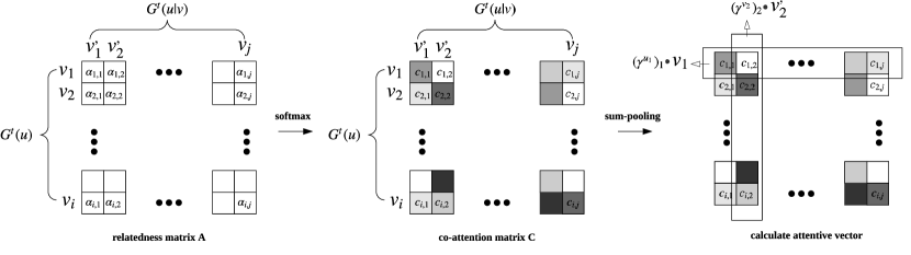
Figure 3. The processes of calculating the co-attention values. First, calculate relatedness matrix $A$; Second, softmax over the whole matrix $A$ and get the co-attention matrix $C$; Lastly, use sum pooling along rows and columns to get attentive vector and use the vector to weighted sum over objects in (co-)interaction set.

3. Methodology

In this section, we present our proposed model SCoRe (Sequential Collaborative Recommender) in detail. We first introduce the high-order collaborative relation mining through cross neighbor modeling, and then we describe the dual sequence modeling in an interactive manner. Furthermore, we analyze the time complexity of the proposed model.

3.1. High-Order Collaborative Relation Mining

In this section, we describe the proposed Co-Attention Network for handling the complex relations across the neighbors of interaction set and co-interaction set.

3.1.1. Cross Neighbor Co-Attention Network

At each time slice $t$, we use Co-Attention Network to capture the complex relations across neighbors in interaction and co-interaction sets.

One of the key parts of recent success of recommendation models (Song et al., 2019; Wu et al., 2019b; Zhou et al., 2018a) are the attention mechanism which attributes different credits to different item representations or temporal representations (e.g. hidden states of RNNs). The attentive weight of a user interacted item $v_{j}$ w.r.t target item $v$ is calculated following the paradigm as,

(9) $$\alpha_{v_{j},v}=Attn(r(v_{j}),v),v_{j}\in\bm{G}(u),$$

where the $Attn(\cdot)$ function can be various, $r(\cdot)$ is representation of $v_{j}$ which could be embedding or hidden states. The calculated $\alpha_{v_{j},v}$ measures the correlation (e.g. similarity) between $v_{j}$ and $v$. This paradigm only focuses on the relations between user interacted items and single target item $v$. But there are many neighboring items of $v$ (those items in $\bm{G}(u|v)$), so we could calculate neighbor-to-neighbor correlations between items in $\bm{G}(u|v)$ and those in $\bm{G}(u)$. In this way, the relation between target $u$ and $v$ can be modeled with more resourceful information.

To model this cross neighbor collaborative relations, we propose Co-Attention Network, which is illustrated in Figure 3. We not only consider the relatedness between the user interacted items and the target item, but also take the relatedness across user interacted items and the collaborative neighbors of the target item into account.

At each time slice, we calculate a co-attention relatedness matrix, $A^{\text{item}}_{t}\in R^{S\times S}$, each element of which is calculated as

(10) $$\alpha_{i,j}^{t}=\sigma(\bm{w}_{1}^{T}[\bm{v}_{i},\bm{v}_{j},\bm{v}]+b),v_{i}\in\bm{G}^{t}(u),v_{j}\in\bm{G}^{t}(u|v)$$

where $\bm{v}$ is the embedding of the target item $v$, $\sigma$ is the ReLU activation function $ReLU(x)=max(0,x)$ and $S$ is the number of items in $\bm{G}^{t}(u)$ and $\bm{G}^{t}(u|v)$. As the objects in $\bm{G}^{t}(u)$ and $\bm{G}^{t}(u|v)$ are all items, we denote this relatedness matrix as $A^{\text{item}}_{t}$. Followed by a softmax operation, we get the co-attention matrix $C^{\text{item}}_{t}$, each element of which is calculated as,

(11) $$c_{i,j}^{t}=\frac{\exp(\alpha_{i,j}^{t})}{\sum_{m,n}\exp(\alpha_{m,n}^{t})}.$$

Symmetrically, we could calculate each element of $A^{\text{user}}_{t}$ as

(12) $$\alpha_{i,j}^{t}=\sigma(\bm{w}^{T}_{2}[\bm{u}_{i},\bm{u}_{j},\bm{u}]+b),u_{i}\in\bm{G}^{t}(v),u_{j}\in\bm{G}^{t}(v|u)$$

and $C^{\text{user}}_{t}$ using the softmax operation described in Eq. (11).

In this way, we could capture cross neighbor relations which are more complex and resourceful than the original paradigm described in Eq. (9).

3.1.2. high-order Information Aggregation

In collaborative filtering (CF) models (Koren, 2008; He et al., 2017; Cheng et al., 2018) and sequential recommendation models (Hidasi et al., 2016; Tang and Wang, 2018; Zhou et al., 2018a), we only use the user (item) directly interacted items (users) to represent a user (item) which may cause a narrow understanding of user or item properties.

However, in previous section, by incorporating the information of co-interaction sets, not only could we model the cross neighbor collaborative relations but integrate high-order information by summarizing the co-interaction set. By integrating these co-interaction objects, we could enrich the representation of target user $u$ and item $v$.

By sum pooling (SP) along the rows or columns of the two co-attention matrix $C^{\text{item}}_{t}$ and $C^{\text{user}}_{t}$, we could get four attentive vector,

(13) $$\bm{\gamma}_{t}^{u_{1}}=SP(\{C^{\text{item}}_{ij}\}_{j=1}^{S}),$$

(14) $$\bm{\gamma}_{t}^{v_{2}}=SP(\{C^{\text{item}}_{ij}\}_{i=1}^{S}),$$

(15) $$\bm{\gamma}_{t}^{u_{2}}=SP(\{C^{\text{user}}_{ij}\}_{j=1}^{S}),$$

(16) $$\bm{\gamma}_{t}^{v_{1}}=SP(\{C^{\text{user}}_{ij}\}_{i=1}^{S}).$$

We denote the embeddings of interaction set and co-interaction set for $u$ and $v$ at $t$-th time slice as $\bm{U}_{t}^{1}\in R^{S\times d}$ (interaction), $\bm{U}_{t}^{2}\in R^{S\times d}$ (co-interaction), $\bm{V}_{t}^{1}\in R^{S\times d}$, $\bm{V}_{t}^{2}\in R^{S\times d}$ respectively, where $d$ is the dimension of the embedding and $S$ is the size of (co-)interaction set. The aggregated representation of $u$ and $v$ at $t$-th time slice are

(17) $$\bm{u}^{agg}_{t}=[{\bm{U}_{t}^{1}}^{T}\bm{\gamma}_{t}^{u_{1}},{\bm{U}_{t}^{2}}^{T}\bm{\gamma}_{t}^{u_{2}}]$$

(18) $$\bm{v}^{agg}_{t}=[{\bm{V}_{t}^{1}}^{T}\bm{\gamma}_{t}^{v_{1}},{\bm{V}_{t}^{2}}^{T}\bm{\gamma}_{t}^{v_{2}}].$$

3.2. Interactive Dual Sequence Modeling

In this section, we describe our approach on temporal dynamics modeling. We conduct a dual sequence modeling method which considers both user-side and item-side sequences and interactively models the relations among two sequences of synchronized time slice.

3.2.1. Temporal Dynamics Modeling

At each time slice, we get the aggregated representations of target user $u$ and target item $v$ as $\bm{u}_{t}^{agg}$ and $\bm{v}_{t}^{agg}$ respectively following the co-attention mechanism in Section 3.1. After that we get two sequences $U$ and $V$, which are the sequences of target user’s and item’s aggregated representation at different time respectively. For simplicity, we denote $\bm{u}_{t}=\bm{u}_{t}^{agg}$ and $\bm{v}_{t}=\bm{v}_{t}^{agg}$ thus

(19) $$U=\{\bm{u}_{1},\bm{u}_{2},...,\bm{u}_{T}\}~{},V=\{\bm{v}_{1},\bm{v}_{2},...,\bm{v}_{T}\}.$$

We use two recurrent neural network models to model the temporal dynamics for user-side and item-side respectively. And we implement each recurrent cell as Gated Recurrent Unit (Cho et al., 2014) (GRU). Each GRU unit takes the corresponding representation $\bm{u}_{t}$ (or $\bm{v}_{t}$) at each time step and the hidden state $\bm{h}_{t-1}$ from the last time step, and then calculates as

(20) $$\bm{z}_{t}^{u}= ~{}\sigma(\overline{\bm{W}}_{z}^{u}\bm{u}_{t}+\overline{\bm{U}}_{z}\bm{h}_{t-1}^{u}+\overline{\bm{b}}_{z}^{u})$$

$$\bm{r}_{t}^{u}= ~{}\sigma(\overline{\bm{W}}_{r}^{u}\bm{u}_{t}+\overline{\bm{U}}_{r}\bm{h}_{t-1}^{u}+\overline{\bm{b}}_{r}^{u})$$

$$\bm{h}_{t}^{u}= ~{}(1-\bm{z}_{t}^{u})\odot\bm{h}_{t-1}^{u}$$

$$~{}~{}~{}~{}~{}~{}~{}~{}~{}~{}~{}~{}~{}~{}~{}~{}~{}+\bm{z}_{t}^{u}\odot\tanh(\overline{\bm{W}}_{h}^{u}\bm{u}_{t}+\overline{\bm{U}}_{h}^{u}(\bm{r}_{t}^{u}\odot\bm{h}_{t-1}^{u})+\overline{\bm{b}}_{h}^{u})~{},$$

where $\odot$ is the element-wise product operator.

The item-side temporal dynamics are modeled in the same way. Till now, we’ve got user-side and item-side sequence of temporal representations: $\{\bm{h}_{1}^{u},\bm{h}_{2}^{u},...,\bm{h}_{T}^{u}\}$ and $\{\bm{h}_{1}^{v},\bm{h}_{2}^{v},...,\bm{h}_{T}^{v}\}$.

3.2.2. Interactive Attention Mechanism of Dual Sequence

As illustrated in Figure 4, different time slice has different impact on the final prediction at $(T+1)$. And hereby we introduce our Interactive Attention Mechanism. Unlike the attention mechanism in (Zhou et al., 2018a) and (Zhou et al., 2018b) which uses the target item to query the interacted items sequence, we utilize dual sequences information at the same time interactively to weigh across different time slice. The attention value of each time slice $\beta_{t}$ is calculated as,

(21) $$relation_{t}=R([\bm{h}_{t}^{u},\bm{h}_{t}^{v},\bm{\gamma}_{t}^{u_{1}},\bm{\gamma}_{t}^{v_{2}},\bm{\gamma}_{t}^{u_{2}},\bm{\gamma}_{t}^{v_{1}}],[\bm{u},\bm{v}])$$

(22) $$\beta_{t}=\frac{\exp(relation_{t})}{\sum_{i=1}^{T}\exp(relation_{i})}$$

where R is a three-layer MLP with ReLU activation function.

And the final representations of user-side and item-side sequences are

(23) $$\bm{r}_{u}=\sum_{t=1}^{T}\beta_{t}\bm{h}_{t}^{u},~{}~{}~{}~{}\bm{r}_{v}=\sum_{t=1}^{T}\beta_{t}\bm{h}_{t}^{v}$$

It is natural that we consider both side information to calculate attention, because the cross neighbor relations modeling described in Section 3.1 utilizes both user-side neighbors and item-side neighbors. As a result, we consider using both sides representations of synchronized time slice to interactively calculate attentive value. In this way, the modeling of two sequences are highly correlated.

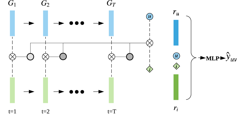
Figure 4. Temporal Interactive Dual Sequence Modeling of SCoRe.

3.3. Final Prediction and Loss Functions

The predicted probability of interaction between the target user and the target item is calculated as

(24) $$\hat{y}=f(\bm{r}_{u},\bm{r}_{v},\bm{u},\bm{v};\bm{\Theta}),$$

where $f$ is implemented as a multi-layer perceptron with the ReLU activation function. The parameters set of the MLP is $\bm{\Theta}$. The inference procedure is illustrated in Figure 4.

As for the loss function, we take an end-to-end training and introduce (i) the widely used cross entropy loss $\mathcal{L}_{\text{ce}}$ (Ren et al., 2018b; Zhou et al., 2018b, a) over the whole training dataset and (ii) the parameter regularization $\mathcal{L}_{\text{r}}$. We utilize Adam algorithm for optimization. Thus the final loss function is

(25) $$\operatorname*{arg\,min}_{\bm{\Theta},\bm{\Phi}} =\mathcal{L}_{\text{ce}}+\lambda\mathcal{L}_{r}$$

$$=-\sum_{s}\big{[}y_{s}\log\hat{y}_{s}+(1-y_{s})\log(1-\hat{y}_{s})\big{]}$$

$$+\frac{1}{2}\lambda\left(\|\bm{\Theta}\|_{2}^{2}+\|\bm{\Phi}\|_{2}^{2}\right)~{},$$

where $\bm{\Phi}$ includes the parameters in GRUs, $\bm{w}_{1}$, $\bm{w}_{2}$ in Co-Attention Network and the parameters of the three-layer MLP $R$ in the Interactive Attention Mechanism.

3.4. Model Efficiency

In this section, we analyze the computational complexity of our SCoRe model. From the previous sections, we can tell that the forward inference of SCoRe can be regarded as two relatively separate parts. The first part is the cross neighbor collaborative relations modeling, which can be paralleled conducted for each time slice. The cost of it can be viewed as a constant $O(C_{co-atten})$ as the co-attention network conduct single layer non-linear transformation, softmax and sum-pooling operations. The second part is the GRU temporal modeling. We assume the average time performance of the GRU is a constant $O(C_{GRU})$ which is related to the implementation of the GRU module yet can be parallelly executed through GPU processor. Recall that we have $T$ time slices, thus the time complexity of temporal inference is $O(T\cdot C_{GRU})$. Therefore the overall time complexity of SCoRe is $O(C_{co-atten})+O(T\cdot C_{GRU})=O(T\cdot C_{GRU})$ which is the time complexity of ordinary recurrent neural networks.

The inference time complexity is acceptable since several implementations sharing similar execution complexity have been adopted online (Wu et al., 2016; Zhou et al., 2018a), which indicates online inference efficiency for our SCoRe model in some extent.

4. Experiments

In this section, we present the details of the experiment setups and the corresponding results. To illustrate the effectiveness of our proposed model, we compare it with some strong baselines on sequential recommendation task. Moreover, we have published our reproductive code.

We start with three research questions (RQ) to lead the experiments and the following discussions.

• Compared to the baseline models, does SCoRe achieve state-of-the-art performance in sequential recommendation task?

• What is the influence of different components in SCoRe? Are the proposed co-attention network and interactive attention necessary for improving performance?

• What patterns does the proposed model capture for the final recommendation decision?

4.1. Experimental Setups

In this part, we describe our experiment setups including datasets with preprocessing method, some important implementation details, evaluation metrics and the compared baselines.

4.1.1. Datasets

We use three real-world large-scale datasets to evaluate all the compared models. The dataset statistics have been shown in Table  2.

CCMR:

(Cao et al., 2016) is a dataset consists of movie rating (from integer score 1 to 5) logs collected from Douban, which is one of China’s largest movie review websites. The data is collected and dumped in May 2015.

Taobao:

(Zhu et al., 2018) is a dataset consisting of user behavior data collected from Taobao, one e-commerce platform in China. It contains user behaviors from November 25 to December 3, 2017 of several behavior types including click, purchase, add to cart and item favoring.

Tmall:

is provided by Alibaba Group which contains user behavior history on Tmall e-commerce platform from May 2015 to November 2015.

Dataset Preprocessing. We cut the time line into total $T$ time slices with the specific time interval as shown in Table 2. And for each time slice, we use the interaction records within it to construct interaction and co-interaction set for both user and item. Here we use a simple way to do time slicing, we leave finer segmentation strategy in future work.

Table 2. The dataset statistics.

Dataset	Users #	Items #	Interaction #	Time slices $T$	Time interval $\Delta T$
CCMR	4,920,695	190,129	283,775,314	41	90 days
Taobao	987,994	4,162,024	100,150,807	9	1 day
Tmall	424,170	1,090,390	54,925,331	13	15 days

Positive & Negative Samples. To evaluate the recommendation performance, we use one positive item and sample 100 negative items at the prediction time $(T+1)$ for each user in all three datasets. For Tmall and Taobao datasets, as we only have the positive user feedbacks (click, buying, etc.), we have to randomly sample the negative items. As for CCMR datasets, we regard items whose ratings are 5 or 4 as positive items and those whose ratings are 1,2 or 3 as negative items. If a user does not have enough negative items, we use random sampling to generate negative items for her. The positive items in CCMR form the behavior sequence.

Train & Test Splitting. The training set contains the sequential behaviors from the first to the $(T-2)$th time slice, we use the interactions history from 1 to $(T-3)$ to predict in $(T-2)$. For the validation set, we use the interactions data from 1 to $(T-2)$ to predict in $(T-1)$. In testing set, interactions data from 1 to $(T-1)$ are used to predict in $T$.

Implementation Details. It is common that the target user doesn’t have any interaction record in a time slice, and similarly, the target item may be not visited by any user in a time slice. To handle this issue, we use a unified embedding vector to represent the situation.

We set the size of interaction set to $S$ which can be regarded as a hyperparameter. For simplicity, the size of co-interaction set is $S$ too. If there are more than $S$ objects in a set, we use random sampling. If there are less than $S$ objects (say $k$ ($<S$) objects), we random sample $(S-k)$ times among the original set.

4.1.2. Evaluation Metrics

Three evaluation metrics are used and all of them are widely used in recommendation tasks.

HR@k (Hit Ratio@k) measures the proportion of samples that the positive item is among the top-k in all test cases which is computed as,

(26) $$HR@k=\frac{1}{|\mathcal{U}|}\sum_{u\in\mathcal{U}}\mathbb{I}(R_{u,v}\leq k),$$

where $R_{u,v}$ is the ranking position of the user $u$’s interacting with item $v$, and $\mathbb{I}$ is the indicator function.

NDCG@k (Normalized Discounted Cumulative Gain) is a position-aware metric which assigns larger weights on higher ranks of the positive item, which is calculated as,

(27) $$NDCG@k=\frac{1}{|\mathcal{U}|}\sum_{u\in\mathcal{U}}\frac{2^{\mathbb{I}(R_{u,v}\leq k)}-1}{log(R_{u,v}+1)}.$$

MRR (Mean Reciprocal Rank) is another position-aware metric that is calculated as,

(28) $$MRR=\frac{1}{|\mathcal{U}|}\sum_{u\in\mathcal{U}}\frac{1}{R_{u,v}}.$$

As HR@1 is equal to NDCG@1, so in this work, we report HR@{1,5,10}, NDCG@{5,10} and MRR in detail.

4.1.3. Compared Baselines

To illustrate the effectiveness of our model, we compare SCoRe with two CF models, three single sequence recommendation models and two dual sequence models. We follow (Zhou et al., 2018a) that all the models take the input sparse features and feed them through an embedding layer for the subsequent inference.

The first group of models are CF models:

• (Koren, 2008) is a hybrid method of latent factor model and neighbor-based model which is the fundamental approach of collaborative filtering recommendation. It regards all the sequential behaviors as a whole and ignores the temporal dynamics.

• (Cheng et al., 2018) is the state-of-the-art CF method which utilizes deep neural networks to capture complex non-linear interaction patterns from both user-side and item-side.

The second group contains sequential recommendation methods that utilize single user-side sequence, which are based on RNNs, CNNs, or Transformer architecture:

• (Hidasi et al., 2016) bases on GRU and it is the first work using the recurrent cell to model sequential user behaviors.

• (Tang and Wang, 2018) is based on CNNs that uses horizontal and vertical convolutional filters to capture user behavior patterns at different scales.

• (Kang and McAuley, 2018) bases on Transformer (Vaswani et al., 2017), it only uses self-attention mechanism without recurrent architecture. It achieves very competitive performance in sequential recommendation task.

The third group is dual sequence recommendation models.

• (Wu et al., 2017) is the first RNN-based model that considers both the user- and item-side sequence. It uses sum-pooling to aggregate the information inside a time slice.

• (Wu et al., 2019a) feed the user-side and item-side sequence respectively into two identical sequential models, and let the two models play a game with each other where one model will use the predicted score of the other model as feedback to guide the training.

• is our proposed model which is described in Section 3.

Table 3. Performance comparison against baseline models. Bold values are the best in each row, while the second best values are underlined. Improvements over baselines are statistically significant with $p$ ¡ 0.01. (HR, NDCG, MRR: the higher, the better)

Dataset	Metric	Group 1		Group 2			Group 3
		SVD++	DELF	GRU4Rec	Caser	SASRec	RRN	DEEMS	SCoRe
CCMR	HR@1	0.0797	0.0755	0.0739	0.0845	0.0817	0.0739	0.0968	0.1035
	HR@5	0.1865	0.2255	0.2477	0.2469	0.2480	0.2214	0.2444	0.2518
	HR@10	0.2686	0.3422	0.3494	0.3663	0.3613	0.3431	0.3599	0.3688
	NDCG@5	0.1340	0.1638	0.1689	0.1736	0.1779	0.1733	0.1776	0.1891
	NDCG@10	0.1604	0.2051	0.1985	0.2113	0.2128	0.2060	0.2115	0.2167
	MRR	0.1516	0.1750	0.1706	0.1829	0.1893	0.1799	0.1896	0.1954
Taobao	HR@1	0.1947	0.3381	0.3439	0.3562	0.3510	0.3204	0.3255	0.3688
	HR@5	0.4489	0.6077	0.6035	0.6085	0.6159	0.6220	0.6478	0.6816
	HR@10	0.5933	0.7084	0.7189	0.7224	0.7371	0.7620	0.7517	0.8068
	NDCG@5	0.3256	0.4731	0.4866	0.5005	0.5101	0.4779	0.4814	0.5339
	NDCG@10	0.3723	0.5089	0.5139	0.5174	0.5199	0.5233	0.5476	0.5745
	MRR	0.3224	0.4405	0.4617	0.4744	0.4818	0.4615	0.4988	0.5121
Tmall	HR@1	0.3447	0.3386	0.3501	0.3588	0.3622	0.3634	0.3669	0.3770
	HR@5	0.5594	0.5636	0.5727	0.5712	0.5819	0.7310	0.7331	0.7381
	HR@10	0.6554	0.6562	0.6646	0.6662	0.6686	0.8378	0.8373	0.8479
	NDCG@5	0.4589	0.4654	0.4784	0.4768	0.4843	0.5594	0.5565	0.5693
	NDCG@10	0.4901	0.4986	0.5080	0.5074	0.5124	0.5942	0.5951	0.6051
	MRR	0.4527	0.4669	0.4741	0.4730	0.4778	0.5256	0.5259	0.5363

4.2. Evaluation Results: RQ1

The experimental results are shown in Table 3, we find several observations as below.

By comparing the performance of SCoRe  and other baseline models, it outperforms baselines by 28.9% to 3.1%, 58.8% to 2.7% and 18.5% to 2.0% on MRR in CCMR, Taobao and Tmall dataset, respectively. And it also shows significant improvements on the other metrics so SCoRe  achieves the state-of-the-art performance in sequential recommendation task.

For the models in Group 1, they do not consider the temporal dynamics of user behaviors thus perform not so good as models in Group 2 and 3. DELF uses both user-side and item-side interaction information so it achieves better performance than SVD++ which only utilizes user-side information.

By comparing the performance of Group 2 and 3, we find in Tmall and Taobao dataset that, Group 3 outperforms Group 2. But over CCMR dataset, SASRec and Caser are better than Group 3. As shown in Table 2, Tmall and Taobao has a lot more items than CCMR, which makes ranking items more difficult in Tmall and Taobao. So it is more important on these two datasets to take item-side sequence into consideration because it gives the models more information than just using single user-side sequence.

DEEMS performs better than RRN in many cases which means the two player game of dual sequence in DEEMS is effective and show the potential of finer design on dual modeling.

Influence from the size of (co-)interaction set. We vary the size of (co-)interaction set to further investigate the robustness of SCoRe. For simplicity, we set interaction and co-interaction set to have same size in dual side. The results on Tmall and Taobao dataset are shown in Figure 5. We find that when size increases, the performance is improved at first because that the larger the size is, the more information it contains. And when the size continues to increase, the performances begin to drop which indicates that too much noise and useless information is introduced.

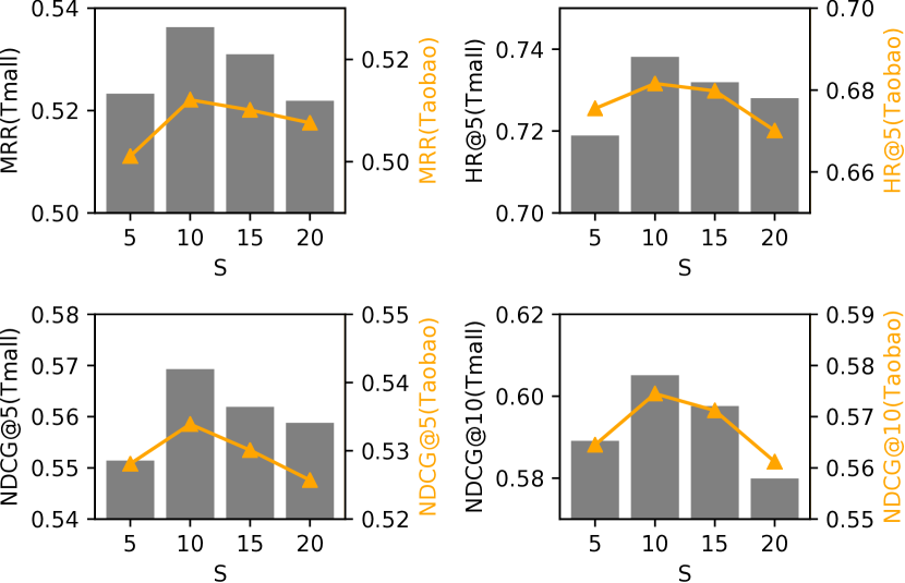
Figure 5. Performance comparision on different size $S$ of (co-)interaction set on Tmall and Taobao dataset.

4.3. Ablation Study: RQ2

In this section, we conduct some ablation studies to investigate the effectiveness of three important components of SCoRe : (1) Interactive Attention Mechanism in dual sequence modeling; (2) Co-Attention Network for cross neighbor relation mining and aggregation; (3) The consideration of using both user-side and item-side.

Table 4. Performance comparison of ablation study.

Dataset	Metric	models
		RIA	RCA	User	Item	SCoRe
CCMR	HR@10	0.3667	0.3461	0.3491	0.3218	0.3688
	NDCG@10	0.2098	0.2077	0.2012	0.1892	0.2167
	MRR	0.1872	0.1795	0.1782	0.1567	0.1954
Taobao	HR@10	0.7888	0.7702	0.7678	0.7453	0.8068
	NDCG@10	0.5436	0.5286	0.5192	0.5001	0.5745
	MRR	0.4785	0.4669	0.4652	0.4495	0.5121
Tmall	HR@10	0.8467	0.8406	0.8355	0.8122	0.8479
	NDCG@10	0.6030	0.5903	0.5843	0.5671	0.6051
	MRR	0.5352	0.5289	0.5192	0.5085	0.5363

We set four comparative settings, and the performances of them have been shown in Table 4. The details of the four settings are listed as below.

• RIA (Remove Interactive Attention) removes the attention part described in 3.2.2 and set the final sequential representations of target user and item as $\bm{r}_{u}=h_{T}^{u}$ and $\bm{r}_{v}=h_{T}^{v}$ of Eq. (23).

• RCA (Remove Co-Attention) removes the co-attention network and uses simply sum pooling to aggregate neighbor information in interaction and co-interaction set.

• User only uses the user-side sequence to do final prediction, as $\hat{y}=f(\bm{r}_{u},\bm{u},\bm{v};\bm{\Theta})$.

• Item only uses the item-side sequence to do final prediction, as $\hat{y}=f(\bm{r}_{v},\bm{u},\bm{v};\bm{\Theta})$.

Except for the changes mentioned above, the other parts of the models and experimental settings remain identical to ensure the fairness of comparison.

From Table 4 we can find that (1) SCoRe performs the best indicating the efficacy of different components of the model. (2) the performance decreases more when removing co-attention than interactive attention which means the cross neighbor relation modeling is more important and fundamental to SCoRe’s performance. (3) Using single sequence hurt the performance badly and item-side is harder to model compared to user-side thus have worse performance.

4.4. Case Study: RQ3

In this section, we further investigate what patterns SCoRe captures by studying and visualizing a specific case sampled from the CCMR dataset. In Figure 6, we plot the prediction of user-item pair (u36, m1911) where m1911 is the movie American Sniper. The ground truth is $y=1$, we plot the Caser and SCoRe  predictions which are $\hat{y}_{\text{caser}}=0.312$ and $\hat{y}_{\text{{SCoRe}}}=0.891$ respectively. By looking into the user behavior sequence, we find the reason of SCoRe’s better prediction result.

The user’s recent behaviors are favouring comedy, cartoon or fiction, as illustrated in the upper part of Figure 6 which are not very relevant to the target item American Sniper which is a biographical and action movie. So it is natural that models like Caser tend to give lower prediction score.

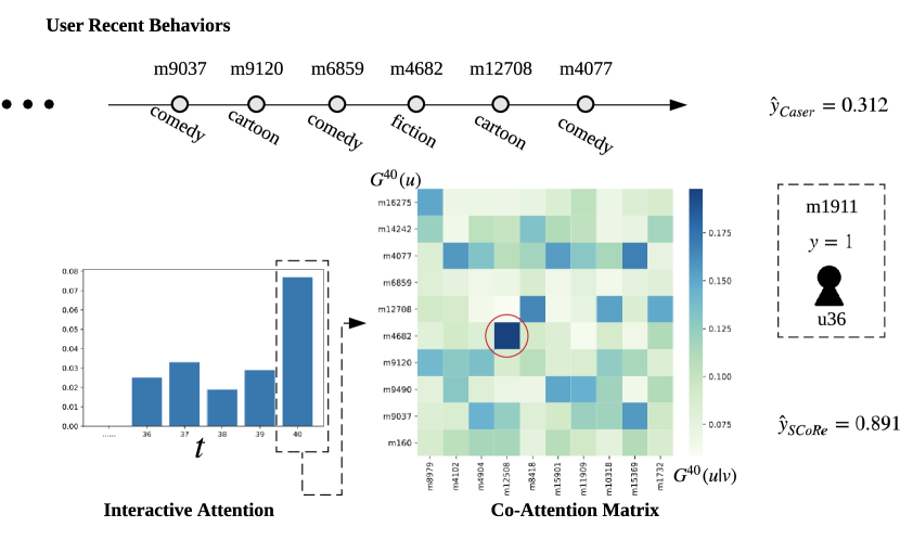
Figure 6. Case study of Caser and SCoRe. We plot user u36’s recent behaviors, interactive attention values and co-attention matrix $C^{\text{item}}_{40}$ of time slice 40 of SCoRe.

However, we plot the interactive attention value of recent time slices of SCoRe and find the 40-th slice have higher attention value. So we further plot the co-attention matrix of this time slice $C^{\text{item}}_{40}$. We find m4682 (Interstellar, fiction and adventure) of $\bm{G}^{40}(u)$ has high relation with m12508 (007:Casino Royal, action and fiction) of $\bm{G}^{40}(u|v)$. Movie m12508 is more relevant to the user’s interest, and its representation is aggregated to the item-side, so it is reasonable that SCoRe has the ability to give the target item higher predicted probability score, which has precisely been interacted by the target user in the test data.

5. Related Work

5.1. Collaborative Filtering

In recommender system literatures, the most widely used method is collaborative filtering (Goldberg et al., 1992), which learns from the historical user-item interactions without exogenous information about items or users. It recommends according to the modeled user preferences, e,g., clicks (Qu et al., 2016; Agarwal et al., 2009) and ratings (Koren, 2009), over the items. Many works (Koren et al., 2009; Salakhutdinov and Mnih, 2007; Yang et al., 2012; Zhang et al., 2013) have been proposed based on collaborative filtering. Among them, latent factor models play a key role in CF methods, ranging from pLSA (Hofmann, 2004) and Latent Dirichlet Allocation (Blei et al., 2003) to SVD-based models (Koren, 2008; Chen et al., 2012) and factorization machines (Rendle, 2010). Nowadays, deep neural network (DNN) has attracted huge attentions in recommender systems because of its effective feature extraction and end-to-end model training with satisfying generalization (Zhang et al., 2017). Some DNN methods (He et al., 2017, 2018; Qu et al., 2016) are proposed for latent factor collaborative filtering. However, almost all of these approaches, either conventional matrix factorization methods or deep models, lack of temporal pattern mining.

5.2. Sequential Recommendation

Recently, sequential recommendation has drawn huge attention since the sequences of user behaviors have rich information for the user interests, especially for concept drifting (Widmer and Kubat, 1996), long-term behavior dependency (Koren, 2009; Ren et al., 2019), periodic patterns (Ren et al., 2018a), etc.

There are three categories for sequential recommendation. The first one is from the view of temporal collaborative filtering (Koren, 2009) with the consideration of drifting user preferences. The second stream is based on Markov-chain methodology (Rendle et al., 2010; He and McAuley, 2016; He et al., 2016) which implicitly models the user state dynamics and derive the outcome behaviors. The third school is based on deep neural networks, such as recurrent neural networks (RNNs) (Hidasi et al., 2016; Hidasi and Karatzoglou, 2018; Wu et al., 2017; Jing and Smola, 2017; Liu et al., 2016; Beutel et al., 2018; Villatel et al., 2018) and convolutional neural networks (CNNs) regarding the behavior history as an image (Tang and Wang, 2018; Kang and McAuley, 2018). However, most of these methods only care about user’s interest drifting and do not consider the sequential patterns of items, which also deliver rich information for user-item matching. Models like (Wu et al., 2017, 2019a) considers both sequences but in a relatively independent way, which leaves space for finer design of dual sequence modeling. Furthermore, most of these sequential models only care about user’s own interaction history while ignoring the information that could be found in similar users or items. And thus the sequential models may suffer from narrowness of recommendation.

6. Conclusion and Future Work

In this paper, we propose SCoRe, a model that utilizes and aggregates high-order collaborative information using cross neighbor modeling to improve representation learning and collaborative relation mining. Furthermore, we propose an interactive attention mechanism to model the user-side and item-side sequences. In this way, dual sequence modeling captures temporal dynamics from both user and item-side and significantly facilitate final recommendation performance.

For the future work, we plan to further investigate on the time segmentation strategy of the evolving sequential interactions and its influence to the recommendation performance. We also seek to deploy our method on the real-world recommender systems.

Acknowledgement. The corresponding author Weinan Zhang thanks the support of National Natural Science Foundation of China (61702327, 61772333, 61632017) and Shanghai Sailing Program (17YF1428200).

References

- (1)
- Agarwal et al. (2009) Deepak Agarwal, Bee-Chung Chen, and Pradheep Elango. 2009. Spatio-temporal models for estimating click-through rate. In WWW.
- Beutel et al. (2018) Alex Beutel, Paul Covington, Sagar Jain, Can Xu, Jia Li, Vince Gatto, and Ed H Chi. 2018. Latent Cross: Making Use of Context in Recurrent Recommender Systems. In WSDM.
- Blei et al. (2003) David M Blei, Andrew Y Ng, and Michael I Jordan. 2003. Latent dirichlet allocation. Journal of machine Learning research 3, Jan (2003), 993–1022.
- Cao et al. (2016) Xuezhi Cao, Weiyue Huang, and Yong Yu. 2016. A Complete & Comprehensive Movie Review Dataset (CCMR). In SIGIR. ACM, 661–664.
- Chen et al. (2012) Tianqi Chen, Weinan Zhang, Qiuxia Lu, Kailong Chen, Zhao Zheng, and Yong Yu. 2012. SVDFeature: a toolkit for feature-based collaborative filtering. Journal of Machine Learning Research 13, Dec (2012), 3619–3622.
- Cheng et al. (2018) Weiyu Cheng, Yanyan Shen, Yanmin Zhu, and Linpeng Huang. 2018. DELF: A Dual-Embedding based Deep Latent Factor Model for Recommendation.. In IJCAI. 3329–3335.
- Cho et al. (2014) Kyunghyun Cho, Bart van Merrienboer, Caglar Gulcehre, Dzmitry Bahdanau, Fethi Bougares, Holger Schwenk, and Yoshua Bengio. 2014. Learning Phrase Representations using RNN Encoder–Decoder for Statistical Machine Translation. In EMNLP.
- Goldberg et al. (1992) David Goldberg, David Nichols, Brian M Oki, and Douglas Terry. 1992. Using collaborative filtering to weave an information tapestry. Commun. ACM 35, 12 (1992), 61–70.
- He et al. (2016) Ruining He, Chen Fang, Zhaowen Wang, and Julian McAuley. 2016. Vista: a visually, socially, and temporally-aware model for artistic recommendation. In RecSys.
- He and McAuley (2016) Ruining He and Julian McAuley. 2016. Fusing similarity models with markov chains for sparse sequential recommendation. In ICDM.
- He et al. (2018) Xiangnan He, Xiaoyu Du, Xiang Wang, Feng Tian, Jinhui Tang, and Tat-Seng Chua. 2018. Outer product-based neural collaborative filtering. arXiv preprint arXiv:1808.03912 (2018).
- He et al. (2017) Xiangnan He, Lizi Liao, Hanwang Zhang, Liqiang Nie, Xia Hu, and Tat-Seng Chua. 2017. Neural collaborative filtering. In WWW. 173–182.
- Hidasi and Karatzoglou (2018) Balázs Hidasi and Alexandros Karatzoglou. 2018. Recurrent neural networks with top-k gains for session-based recommendations. CIKM (2018).
- Hidasi et al. (2016) Balázs Hidasi, Alexandros Karatzoglou, Linas Baltrunas, and Domonkos Tikk. 2016. Session-based recommendations with recurrent neural networks. ICLR (2016).
- Hofmann (2004) Thomas Hofmann. 2004. Latent semantic models for collaborative filtering. ACM Transactions on Information Systems (TOIS) 22, 1 (2004), 89–115.
- Jing and Smola (2017) How Jing and Alexander J Smola. 2017. Neural survival recommender. In WSDM.
- Kang and McAuley (2018) Wang-Cheng Kang and Julian McAuley. 2018. Self-Attentive Sequential Recommendation. ICDM (2018).
- Koren (2008) Yehuda Koren. 2008. Factorization meets the neighborhood: a multifaceted collaborative filtering model. In SIGKDD. ACM, 426–434.
- Koren (2009) Yehuda Koren. 2009. Collaborative filtering with temporal dynamics. In KDD.
- Koren et al. (2009) Yehuda Koren, Robert Bell, Chris Volinsky, et al. 2009. Matrix factorization techniques for recommender systems. Computer 42, 8 (2009), 30–37.
- Liu et al. (2016) Qiang Liu, Shu Wu, Diyi Wang, Zhaokang Li, and Liang Wang. 2016. Context-Aware Sequential Recommendation. In ICDM.
- Petrovic et al. (2011) Sasa Petrovic, Miles Osborne, and Victor Lavrenko. 2011. Rt to win! predicting message propagation in twitter. In Fifth International AAAI Conference on Weblogs and Social Media.
- Qu et al. (2016) Yanru Qu, Han Cai, Kan Ren, Weinan Zhang, Yong Yu, Ying Wen, and Jun Wang. 2016. Product-based neural networks for user response prediction. In ICDM.
- Ren et al. (2019) Kan Ren, Jiarui Qin, Yuchen Fang, Weinan Zhang, Lei Zheng, Weijie Bian, Guorui Zhou, Jian Xu, Yong Yu, Xiaoqiang Zhu, et al. 2019. Lifelong Sequential Modeling with Personalized Memorization for User Response Prediction. SIGIR.
- Ren et al. (2018b) Kan Ren, Weinan Zhang, Ke Chang, Yifei Rong, Yong Yu, and Jun Wang. 2018b. Bidding Machine: Learning to Bid for Directly Optimizing Profits in Display Advertising. TKDE (2018).
- Ren et al. (2018a) Pengjie Ren, Zhumin Chen, Jing Li, Zhaochun Ren, Jun Ma, and Maarten de Rijke. 2018a. RepeatNet: A Repeat Aware Neural Recommendation Machine for Session-based Recommendation. arXiv preprint arXiv:1812.02646 (2018).
- Rendle (2010) Steffen Rendle. 2010. Factorization machines. In ICDM.
- Rendle et al. (2010) Steffen Rendle, Christoph Freudenthaler, and Lars Schmidt-Thieme. 2010. Factorizing personalized markov chains for next-basket recommendation. In WWW.
- Rizoiu et al. (2018) Marian-Andrei Rizoiu, Swapnil Mishra, Quyu Kong, Mark Carman, and Lexing Xie. 2018. SIR-Hawkes: Linking epidemic models and Hawkes processes to model diffusions in finite populations. In Proceedings of the 2018 World Wide Web Conference. International World Wide Web Conferences Steering Committee, 419–428.
- Salakhutdinov and Mnih (2007) Ruslan Salakhutdinov and Andriy Mnih. 2007. Probabilistic Matrix Factorization.. In Nips, Vol. 1. 2–1.
- Song et al. (2019) Weiping Song, Zhiping Xiao, Yifan Wang, Laurent Charlin, Ming Zhang, and Jian Tang. 2019. Session-based social recommendation via dynamic graph attention networks. In Proceedings of the Twelfth ACM International Conference on Web Search and Data Mining. ACM, 555–563.
- Tang and Wang (2018) Jiaxi Tang and Ke Wang. 2018. Personalized top-n sequential recommendation via convolutional sequence embedding. In WSDM.
- Vaswani et al. (2017) Ashish Vaswani, Noam Shazeer, Niki Parmar, Jakob Uszkoreit, Llion Jones, Aidan N Gomez, Łukasz Kaiser, and Illia Polosukhin. 2017. Attention is all you need. In Advances in neural information processing systems. 5998–6008.
- Villatel et al. (2018) Kiewan Villatel, Elena Smirnova, Jérémie Mary, and Philippe Preux. 2018. Recurrent Neural Networks for Long and Short-Term Sequential Recommendation. KDD (2018).
- Widmer and Kubat (1996) Gerhard Widmer and Miroslav Kubat. 1996. Learning in the presence of concept drift and hidden contexts. Machine learning 23, 1 (1996), 69–101.
- Wu et al. (2017) Chao-Yuan Wu, Amr Ahmed, Alex Beutel, Alexander J Smola, and How Jing. 2017. Recurrent recommender networks. In WSDM.
- Wu et al. (2019a) Qitian Wu, Yirui Gao, Xiaofeng Gao, Paul Weng, and Guihai Chen. 2019a. Dual Sequential Prediction Models Linking Sequential Recommendation and Information Dissemination. In Proceedings of the 25th ACM SIGKDD International Conference on Knowledge Discovery & Data Mining. ACM, 447–457.
- Wu et al. (2019b) Qitian Wu, Hengrui Zhang, Xiaofeng Gao, Peng He, Paul Weng, Han Gao, and Guihai Chen. 2019b. Dual Graph Attention Networks for Deep Latent Representation of Multifaceted Social Effects in Recommender Systems. In The World Wide Web Conference. ACM, 2091–2102.
- Wu et al. (2016) Sai Wu, Weichao Ren, Chengchao Yu, Gang Chen, Dongxiang Zhang, and Jingbo Zhu. 2016. Personal recommendation using deep recurrent neural networks in NetEase. In ICDE.
- Yang et al. (2012) Diyi Yang, Tianqi Chen, Weinan Zhang, Qiuxia Lu, and Yong Yu. 2012. Local implicit feedback mining for music recommendation. In RecSys. ACM, 91–98.
- Zhang et al. (2017) Shuai Zhang, Lina Yao, and Aixin Sun. 2017. Deep learning based recommender system: A survey and new perspectives. arXiv preprint arXiv:1707.07435 (2017).
- Zhang et al. (2013) Weinan Zhang, Tianqi Chen, Jun Wang, and Yong Yu. 2013. Optimizing top-n collaborative filtering via dynamic negative item sampling. In SIGIR. ACM, 785–788.
- Zhou et al. (2018a) Guorui Zhou, Na Mou, Ying Fan, Qi Pi, Weijie Bian, Chang Zhou, Xiaoqiang Zhu, and Kun Gai. 2018a. Deep Interest Evolution Network for Click-Through Rate Prediction. arXiv preprint arXiv:1809.03672 (2018).
- Zhou et al. (2018b) Guorui Zhou, Xiaoqiang Zhu, Chenru Song, Ying Fan, Han Zhu, Xiao Ma, Yanghui Yan, Junqi Jin, Han Li, and Kun Gai. 2018b. Deep interest network for click-through rate prediction. In KDD.
- Zhu et al. (2018) Han Zhu, Xiang Li, Pengye Zhang, Guozheng Li, Jie He, Han Li, and Kun Gai. 2018. Learning Tree-based Deep Model for Recommender Systems. In KDD.