Local Search for Group Closeness Maximization
on Big Graphs

Abstract

In network analysis and graph mining, closeness centrality is a popular measure to infer the importance of a vertex. Computing closeness efficiently for individual vertices received considerable attention. The $\mathcal{NP}$-hard problem of group closeness maximization, in turn, is more challenging: the objective is to find a vertex group that is central as a whole and state-of-the-art heuristics for it do not scale to very big graphs yet.

In this paper, we present new local search heuristics for group closeness maximization. By using randomized approximation techniques and dynamic data structures, our algorithms are often able to perform locally optimal decisions efficiently. The final result is a group with high (but not optimal) closeness centrality.

We compare our algorithms to the current state-of-the-art greedy heuristic both on weighted and on unweighted real-world graphs. For graphs with hundreds of millions of edges, our local search algorithms take only around ten minutes, while greedy requires more than ten hours. Overall, our new algorithms are between one and two orders of magnitude faster, depending on the desired group size and solution quality. For example, on weighted graphs and $k=10$, our algorithms yield solutions of $$12.384\,054\,953\,251\,923$\%$ higher quality, while also being $$793.642\,440\,045\,874\,3$\times$ faster. For unweighted graphs and $k=10$, we achieve solutions within $$99.382\,573\,688\,401\,14$\%$ of the state-of-the-art quality while being $$127.833\,197\,154\,403\,05$\times$ faster.

I Introduction

Identifying important vertices in large networks is one of the main problems in network analysis [1]. For this purpose, several centrality measures have been introduced over the past decades [2]. Among them, one of the most widely-used measures is closeness [3]. For a given vertex $v$, it is defined as the reciprocal of the average shortest-path distance from $v$ to all other vertices. The problem of identifying the $k$ vertices with highest closeness centrality has received significant attention [4, 5, 6]. In graph mining applications, however, it is often necessary to determine a group of vertices that is central as a whole – which is an orthogonal problem shown to be $\mathcal{NP}$-hard [7]. One can view group closeness as special case (on graphs) of the well-known $k$-median problem for facility location. Example applications include: (i) retailers that want to advertise their product via social media; they could select as promoters the group of $k$ members with highest centrality ($\approx$ influence over the other members) [8]; (ii) in P2P networks, shared resources could be placed on $k$ peers so that they are easily accessible by others [9]; (iii) in citation networks, group centrality measures can be employed as alternative indicators for the influence of journals or papers within their field [10].

Everett and Borgatti [11] formalized the concept of centrality for groups of vertices; the closeness of a group $S$ is defined as the reciprocal of the average distance from $S$ to all other vertices of the graph. While exact algorithms to find a group with maximal group closeness are known (e. g., algorithms based on integer linear programming (ILP) [12]), they do not scale to graphs with more than a few thousand edges. Hence, in practice, heuristics are used to find groups with high group closeness on large real-world data sets. For example, Chen et al. [7] proposed a greedy algorithm that heuristically computes a group $S$ with high closeness $C(S)$. To obtain a group of size $k$, it performs $k$ iterations and adds in each iteration the vertex with highest marginal contribution to $S$. It was shown empirically that this greedy algorithm yields solutions of very high quality (within $97\%$ of the optimum) [12] – at least for those small graphs where running a comparison against an exact algorithm is still feasible within a few hours. Due to greedy’s promising quality, Bergamini et al. [12] proposed techniques to speed up the algorithm by pruning, e. g., by exploiting the supermodularity of farness, i. e., $1/C(S)$. Pruning yields a significant acceleration (while retaining the same solution); however, graphs with hundreds of millions of edges still require several hours to complete. Indeed, pruning is most effective when the group is already large. When performing the first addition, however, the greedy algorithm has to perform one (pruned) single-source shorted-path (SSSP) computation for each vertex in the graph to compute its marginal contribution, and this phase scales super-linearly in the size of the graph.

Our Contribution

We present two new local search algorithms for group closeness: the first algorithm, Local-Swap, requires little time per iteration but can only exchange vertices locally. Our second algorithm, Grow-Shrink, is able to perform non-local vertex exchanges, but updating its data structures is more involved. The final result of both algorithms is heuristic, i. e., no approximation guarantee is known. Yet, each iteration of Local-Swap maximizes (in approximation) a lower bound on the objective function, while each iteration of Grow-Shrink locally maximizes the objective function itself. Despite these favorable properties, the time complexity of a single iteration of our algorithms matches the time complexity of a single evaluation of the objective function, i. e., for unweighted graphs, it is linear in the size of the graph.

Our experiments show that our best algorithm, extended Grow-Shrink, finds solutions with a closeness score greater than $$99.382\,573\,688\,401\,14$\%$ of the score of a greedy solution, while being $$127.833\,197\,154\,403\,05$\times$ faster to compute ($k=10$). We see this algorithm as our main contribution for unweighted graphs. When quality is not a primary concern, our other algorithms can further accelerate the computation: For example, the non-extended variant of Grow-Shrink yields solutions for groups of size 10 whose quality is $$91.1$\%$ compared to the state of the art; in this case, it is $$700.2$\times$ faster. The speedup varies between $$927.871\,445\,138\,909$\times$ and $$42.969\,544\,666\,040\,31$\times$ for groups of sizes 5 and 100, respectively.

On weighted graphs, our algorithms even improve both the quality and the running time performance compared to the state of the art, returning solutions of $$12.384\,054\,953\,251\,923$\%$ higher quality at a speedup of $$793.642\,440\,045\,874\,3$\times$ ($k=10$). Other trade-offs between quality and performance are possible and discussed in Section III.

II Local Search for Group Closeness

Let $G=(V,E)$ be an undirected connected graph. We allow both unweighted and positively weighted graphs $G$. Subsets $S\subseteq V$ are called groups. The farness of any given group $S$ is defined as:

$$f(S)=\sum_{v\in V\setminus S}\mathrm{dist}(S,v).$$

Here, $\mathrm{dist}(S,v)$ refers to the minimal shortest-path distance from any $s\in S$ to $v$ in $G$. Furthermore, the (group) closeness of $S$ is defined as $C(S)=|V|/f(S)$, i. e., $C(S)$ is the reciprocal of the average distance of all vertices in $V\setminus S$ to the nearest vertex in $S$. Recall that determining the group $S^{*}$ that maximizes $C$ over all groups $S$ with $|S|\leq k$ is known to be $\mathcal{NP}$-hard [7]; we are not aware of any algorithm with a bounded approximation ratio.

We consider the problem of improving the group closeness of a given set $S$ via local search. More precisely, we consider exchanges of vertices from $S$ and $V\setminus S$. Let $u$ be a vertex in $S$ and $v\in V\setminus S$. To simplify the presentation, we use the notation $S^{+v}_{-u}:=(S\setminus\{u\})\cup\{v\}$ to denote the set that is constructed by exchanging $u$ and $v$. We also use the notation $S^{+v}:=S\cup\{v\}$ and $S_{-u}:=S\setminus\{u\}$, to denote vertex additions and removals, respectively.

Note that, as our algorithms can only perform vertex exchanges, they require the construction of an initial set $S$ before the algorithms start. To avoid compromising our algorithms’ running times, we cannot afford a superlinear initialization step. Thus, in all of our local search algorithms, we simply choose the initial $S$ uniformly at random. For large graphs, this initialization can be expected to cover the graph reasonably well. Exploratory experiments revealed that other obvious initialization techniques (such as selecting the $k$ vertices with highest degree) did not improve the performance of the algorithm.

II-A Estimating the Quality of Vertex Exchanges

It is known that a simple greedy ascent algorithm yields results of good quality on real-world graphs [12]. This greedy algorithm starts with an empty set $S$ and iteratively adds vertices $v\in V\setminus S$ to $S$ that maximize $f(S)-f(S^{+v})$. Depending on the input graph and the value of $k$, however, the greedy algorithm might need to evaluate the difference in $f$ for a substantial number of vertices – this computation is rather expensive for large real-world graphs.

The algorithms in this paper aim to improve upon the running time of the greedy algorithm. We achieve this by considering only local vertices for $v$, i. e., vertices that are already “near” $S$. It is clear that selecting only local vertices would decrease the quality of a greedy solution (as the greedy algorithm does not have the ability to eventually correct suboptimal choices). However, this is not necessarily true for our algorithms based on vertex exchanges in Sections II-B and II-C.

To make our notion of locality more concrete, let $B_{S}\subseteq G$ be the DAG constructed by running a SSSP algorithm (i. e., BFS or Dijkstra’s algorithm) from the vertices in $S$. We remark that we work with the full SSSP DAG here (and not a SSSP tree). Here, the vertices of $S$ are all considered as sources of the SSSP algorithm, i. e., they are at distance zero. Furthermore, define

$$\Delta^{-}(v) :=f(S)-f(S^{+v})$$

$$\phantom{:}=\sum_{x\in V\setminus S}\mathrm{dist}(S,x)-\mathrm{dist}(S^{+v},x).$$ (1)

To compute the greedy solution, it seems to be necessary to compute $\Delta^{-}(v)$ exactly for a substantial number of vertices $v$. As discussed above, this seems to be impractical for large graphs. However, a lower bound for $\Delta^{-}(v)$ can be computed from the shortest path DAG $B_{S}$. To this end, let $D_{v}$ be the set of vertices reachable from $v$ in $B_{S}$.

Lemma 1.

It holds that:

$$\Delta^{-}(v)\geq|D_{v}|\cdot\mathrm{dist}(S,v).$$

In the unweighted case, equality holds if $v$ is a neighbor of $S$.

This lemma can be proven from the definition of $B_{S}$. A formal proof can be found in Appendix A.

The bound of Lemma 1 will be used in the two algorithms in Sections II-B and  II-C. Instead of picking vertices that maximize $\Delta^{-}$, those algorithms pick vertices that maximize the right-hand side of Lemma 1, i. e., $|D_{v}|\cdot\mathrm{dist}(S,v)$. The bound is local in the sense that it is more accurate for vertices near $S$: in particular, the reachability sets of vertices in $(V\setminus S)\cap N(S)$ are larger in $G$ than those in $B$, as $B$ does not contain back edges. Unfortunately, computing the size of $D_{v}$ exactly for all $v$ still seems to be prohibitively expensive: indeed, the fastest known algorithm to compute the size of the transitive closure of a DAG (= $\sum|D_{v}|$) relies on iterated (Boolean) matrix multiplication (hence, the best known exact algorithm has a complexity of $\mathcal{O}(n^{2.37})$ [14]). However, it turns out that randomized algorithms can be used to approximate the sizes of $D_{v}$ for all $v$ at the same time. We employ the randomized algorithm of Cohen [15] for this task. In multiple iterations, this algorithm samples a random number for each vertex of the graph $G$, accumulates in each vertex $v$ the minimal random number of any vertex reachable from $v$, and estimates $|D_{v}|$ based on this information.

We remark that since Cohen’s algorithm yields an approximation, but not a lower bound for the right-hand side of Lemma 1, the inequality of the Lemma can be violated in our algorithms; in particular, it can happen that our algorithms pick a vertex $v$ such that $\Delta^{-}(v)<0$. In this case, instead of decreasing the closeness centrality of our current group, our algorithms terminate. Nevertheless, our experiments demonstrate that on real-world instances, a coarse approximation of the reachability set size is enough for Lemma 1 to yield useful candidates for vertex exchanges (see Section II-D5 and Appendix C-B).

II-B Local-Swaps Algorithm

Algorithm 1 Overview of Local-Swaps Algorithm

1:repeat

2:     approximate $|D_{v}|$ for all $V\setminus S$

3:      $(u,v)\leftarrow\operatorname{argmax}_{u\in S,v\in N(u)\setminus S}|D_{v}|-|\Lambda_{u}|$

4:     $S\leftarrow S^{+v}_{-u}$

5:      run pruned BFS from $v$ $\triangleright$ to recompute $f(S)$

6:until previous iteration did not decrease $f(S)$

Let us first focus on unweighted graphs. To construct a fast local search algorithm, a straightforward idea is to allow swaps between vertices in $S$ and their neighbors in $V\setminus S$. This procedure can be repeated until no swap can decrease $f(S)$. Let $u\in S$ be a vertex of the group and let $v\in N(S)\setminus S$ be one of its neighbors outside of the group. To determine whether swapping $u$ and $v$ (i. e., replacing $S$ by $S^{+v}_{-u}$) is beneficial, we have to check whether $f(S)-f(S^{+v}_{-u})>0$, i. e., whether the farness is decreased by the swap. The challenge here is to find a pair $u,v$ that satisfies this inequality (without checking all pairs $u,v$ exhaustively) and to compute the difference $f(S)-f(S^{+v}_{-u})$ quickly. Note that a crucial ingredient that allows us to construct an efficient algorithm is that the distance of $S$ to every vertex $x$ can only change by $\pm 1$ when doing a swap. Hence, we only have to count the numbers of vertices where the distance changes by $-1$ and the number of vertices where it changes by $+1$.

Our algorithm requires a few auxiliary data structures to compute $f(S)-f(S^{+v}_{-u})$. In particular, we store the following:

• the distance $\mathrm{dist}(S,x)$ from $S$ to all vertices $x\in V\setminus S$,

• a set $\lambda_{x}:=\{w\in S:\mathrm{dist}(S,x)=\mathrm{dist}(w,x)\}$ for each $x\in V\setminus S$ that contains all vertices in $S$ that realize the shortest distance from $S$ to $x$,

• the value $|\Lambda_{w}|$ for each $w\in S$, where $\Lambda_{w}:=\{x\in V\setminus S:\lambda_{x}=\{w\}\}$ is the set of vertices for which the shortest distance is realized exclusively by $w$.

Note that the sets $\lambda_{x}$ consume $\mathcal{O}(k|V|)$ memory in total. However, since $k\ll|V|$, this can be afforded even for large real-world graphs. In our implementation, we store each $\lambda_{x}$ in only $k$ bits.

All of those auxiliary data structures can be maintained dynamically during the entire algorithm with little additional overhead. More precisely, after a $u$-$v$ swap is done, $v$ is added to all $\lambda_{x}$ satisfying $\mathrm{dist}(v,x)=\mathrm{dist}(S,x)$; for $x\in V\setminus S$ that satisfy $\mathrm{dist}(v,x)<\mathrm{dist}(S,x)$, the set $\{v\}$ replaces $\lambda_{x}$. $u$ can be removed from all $\lambda_{x}$ by a linear scan through all $x\in V\setminus S$.

Algorithm 1 states a high-level overview of the algorithm. In the following, we discuss how to pick a good swap (line 3 of the pseudocode) and how to update the data structures after a swap (line 5). The running time of the algorithm is dominated by the initialization of $\lambda_{x}$. Thus, it runs in $\mathcal{O}(k|V|+|E|)$ time for each update.

II-B1 Choosing a Good Swap

Because it would be too expensive to compute the exact difference in $f$ for each possible swap, we find the pair of vertices $(u,v)$ with $u\in S$, $v\in N(v)\setminus S$ that maximizes $|D_{v}|\cdot\mathrm{dist}(S,v)-|\Lambda_{u}|=|D_{v}|-|\Lambda_{u}|$. Note that this value is a lower bound for the decrease of $f$ after swapping $u$ and $v$: In particular, Lemma 1 implies that $|D_{v}|$ is a lower bound for the decrease in farness when adding $v$ to $S$. Additionally, $|\Lambda_{u}|$ is an upper bound for the increase in farness when removing $u$ from $S$ (and hence also for the increase in farness when removing $u$ from $S^{+v}$). Thus, we can expect this strategy to yield pairs of vertices that lead to a decrease of $f$. To maximize $|D_{v}|-|\Lambda_{u}|$, for each $v\in V\setminus S$, we compute the neighbor $u\in N(v)\cap S$ that minimizes $|\Lambda_{u}|$ (in $\mathcal{O}(|V|+|E|)$ time). Afterwards, we can maximize $|D_{v}|-|\Lambda_{u}|$ by a linear scan over all $v\in V\setminus S$.

II-B2 Computing the Difference in Farness

Instead of comparing distances, it is sufficient to define sets of vertices whose distance to $S$ is increased or decreased (by 1) by the swap:

$$H^{+}_{u,v} :=\{x\in V:\mathrm{dist}(S,x)<\mathrm{dist}(S^{+v}_{-u},x)\},$$

$$H^{-}_{u,v} :=\{x\in V:\mathrm{dist}(S,x)>\mathrm{dist}(S^{+v}_{-u},x)\}$$

As $\mathrm{dist}(S,x)-\mathrm{dist}(S^{+v}_{-u},x)\in\{-1,0,+1\}$, it holds that:

Lemma 2.

$f(S)-f(S^{+v}_{-u})=|H^{-}_{u,v}|-|H^{+}_{u,v}|$

Fortunately, computing $H^{-}_{u,v}$ is straightforward: this can be done by running a BFS rooted at $v$; the BFS simply counts those vertices $x$ for which $\mathrm{dist}(v,x)<\mathrm{dist}(S,x)$. Hence, to check this condition, we have to store the values of $\mathrm{dist}(S,x)$ for all $x\in V$. We remark that it is not necessary to run a full BFS: indeed, we can prune the search once $\mathrm{dist}(v,x)\geq\mathrm{dist}(S,x)$ (i. e., if the BFS is about to visit a vertex $x$ satisfying this condition, the search continues without visiting $x$). However, as we will see in the following, it makes sense to sightly relax the pruning condition and only prune the BFS if $\mathrm{dist}(v,x)>\mathrm{dist}(S,x)$; this allows us to update our auxiliary data structures on the fly.

$H^{+}_{u,v}$ can be computed from $|\Lambda_{u}|$ with the help of the auxiliary data structures. We note that $H^{+}_{u,v}\subseteq\Lambda_{u}$, as only vertices $x$ where $\mathrm{dist}(S,x)$ is uniquely realized by $u$ (out of all vertices in the group) can have their distance from $S$ increased by the swap. As $H^{+}_{u,v}\cap H^{-}_{u,v}=\emptyset$, we can further restrict this inclusion to $H^{+}_{u,v}\subseteq\Lambda_{u}\setminus H^{-}_{u,v}$, but, in general, $\Lambda_{u}\setminus H^{-}_{u,v}$ will consist of more vertices than just $H^{+}_{u,v}$. More precisely, $\Lambda_{u}\setminus H^{-}_{u,v}$ can be partitioned into $\Lambda_{u}\setminus H^{-}_{u,v}=H^{+}_{u,v}\cup L^{0}_{u,v}$, where $L^{0}_{u,v}:=\{x\in\Lambda_{u}:\mathrm{dist}(u,x)=\mathrm{dist}(v,x)\}$ consists only of vertices whose distance is neither increased nor decreased by the swap. By construction, $L^{0}_{u,v}$ and $H^{+}_{u,v}$ are disjoint. This proves that the following holds:

Lemma 3.

$|H^{+}_{u,v}|=|\Lambda_{u}|-|\Lambda_{u}\cap H^{-}_{u,v}|-|L^{0}_{u,v}|$.

We note that $L^{0}_{u,v}$ (and also $\Lambda_{u}\cap H^{-}_{u,v}$) is completely visited by our BFS. To determine $|L^{0}_{u,v}|$, the BFS only has to count the vertices $x$ that satisfy $\mathrm{dist}(v,x)=\mathrm{dist}(S,x)$ and $\lambda_{x}=\{u\}$. On the other hand, to determine $|\Lambda_{u}\cap H^{-}_{u,v}|$, it has to count the vertices $x$ satisfying $\mathrm{dist}(v,x)<\mathrm{dist}(S,x)$ and $\lambda_{x}=\{u\}$.

II-C Grow-Shrink Algorithm

Algorithm 2 Overview of Grow-Shrink Algorithm

1:repeat

2:      approximate $|D_{v}|$ for all $v\in V\setminus S$

3:     $v\leftarrow\operatorname{argmax}_{v\in V\setminus S}|D_{v}|\cdot d(v)$

4:     $S\leftarrow S^{+v}$

5:      run pruned BFS from $v$ $\triangleright$ to recompute $f(S)$, $d$, $d^{\prime}$

6:      $u\leftarrow\operatorname{argmin}_{u\in S}\sum_{x\in R_{u}}d^{\prime}(x)-d(x)$

7:     $S\leftarrow S_{-u}$

8:      run Dijkstra-like algo. $\triangleright$ to recompute $f(S)$, $d$, $d^{\prime}$

9:until previous iteration did not decrease $f(S)$

The main issue with the swapping algorithm from Section II-B is that it can only exchange a vertex $u\in S$ with one of its neighbors $v\in N(u)\setminus S$. Due to this behavior, the algorithm might take a long time to converge to a local optimum. It also makes it hard to escape a local optimum: indeed, the algorithm will terminate if no swap with a neighbor can improve the closeness.

Our second algorithm lifts those limitations. It also allows $G$ to be a weighted graph. In particular, it allows vertex exchanges that change the distances from $S$ to the vertices in $V\setminus S$ by arbitrary amounts. Computing the exact differences $f(S)-S(S^{+v}_{-u})$ for all possible pairs of $u$ and $v$ seems to be impractical in this setting. Hence, we decompose the vertex exchange of $u$ and $v$ into two operations: the addition of $v$ to $S$ and the removal of $u$ from $S^{+v}$. In particular, we allow the set $S$ to grow to a size of $k+1$ before we shrink the size of $S$ back to $k$. Thus, the cardinality constraint $|S|\leq k$ is temporarily violated; eventually, the constraint is restored again. Fortunately, the individual differences $f(S)-f(S^{+v})$ and $f(S^{+v})-f(S^{+v}_{-u})$ (or bounds for those differences) turn out to be efficiently computable for all possible $u$ and $v$, at least in approximation. We remark, however, that while this technique does find the vertex that maximizes $f(S)-f(S^{+v})$ and the vertex that maximizes $f(S^{+v})-f(S^{+v}_{-u})$, it does not necessarily find the pair of vertices maximizing $f(S)-f(S^{+v}_{-u})$. Nevertheless, our experiments in Section III demonstrate that the solution quality of this algorithm is superior to the quality of the local-swaps algorithm.

In order to perform these computations, our algorithm maintains the following data structures:

• the distance $d(x)$ of each vertex $x\notin S$ to $S$, and a representative $r(x)\in S$ that realizes this distance, i. e., it holds that $\mathrm{dist}(S,x)=\mathrm{dist}(r(x),x)=d(x)$,

• the distance $d^{\prime}(x)$ from $S\setminus\{r(x)\}$ to $x$ and representative $r^{\prime}(x)$ for this distance (satisfying the analogous equality).

Since the graph is connected, these data structures are well-defined for all groups $S$ of size $|S|\geq 1$. Furthermore, the difference between $d^{\prime}(x)$ and $d(x)$ yields exactly the difference in farness when $r(x)$ is removed from the $S$. Later, we will use this fact to quickly determine differences in farness.

We remark that it can happen that $d(x)=d^{\prime}(x)$; nevertheless, $r(x)$ and $r^{\prime}(x)$ are always distinct. Indeed, there can be two distinct vertices $r(x)$ and $r^{\prime}(x)$ in $S$ that satisfy $\mathrm{dist}(r(x),x)=\mathrm{dist}(r^{\prime}(x),x)=\mathrm{dist}(S,x)$. With $R_{u}$ and $R^{\prime}_{u}$, we denote the set of vertices $x\in V\setminus S$ with $r(x)=u$ and $r^{\prime}(x)=u$, respectively.

Algorithm 2 gives a high-level overview of the algorithm. In the following two subsections, we discuss the growing phase (line 2-5) and the shrinking phase (line 6-8) individually. The running time of Grow-Shrink is dominated by the Dijkstra-like algorithm (in line 8). Therefore, it runs in $\mathcal{O}(|V|+|E|\log|V|)$ time per update (when using an appropriate priority queue). The space complexity is $\mathcal{O}(|V|+|E|)$.

II-C1 Vertex additions

When adding a vertex $v$ to $S$, we want to select $v$ such that $f(S^{+v})$ is minimized. Note that minimizing $f(S^{+v})$ is equivalent to maximizing the difference $f(S)-f(S^{+v})=\Delta^{-}(v)$. Instead of maximizing $\Delta^{-}(v)$, we maximize the lower bound $|D_{v}|\cdot\mathrm{dist}(S,v)$. We perform a small number of iterations of the reachability set size approximation algorithm (see Section II-A) to select the vertex $v$ with (approximatively) largest $|D_{v}|$.

After $v$ is selected, we perform a BFS from $v$ to compute $\Delta^{-}(v)$ exactly. As we only need to visit the vertices whose distance to $S^{+v}$ is smaller than to $S$, this BFS can be pruned once a vertex $x$ is reached with $\mathrm{dist}(S,x)<\mathrm{dist}(v,x)$. During the BFS, the values of $d,d^{\prime},r,r^{\prime}$ are updated to reflect the vertex addition: the only thing that can happen here is that $v$ realizes either of the new distances $d$ or $d^{\prime}$.

II-C2 Vertex removals

For vertex removals, we can efficiently calculate the exact increase $\Delta^{+}(u):=f(S_{-u})-f(S)$ in farness for all vertices $u\in S$, even without relying on approximation. In fact, $\Delta^{+}(u)$ is given as:

$$\Delta^{+}(u)=\sum_{x\in R_{u}}d^{\prime}(x)-d(x).$$

We need to compute $k$ such sums (i. e., $\Delta^{+}(u)$ for each $u\in S$); but they can all be computed at the same time by a single linear scan through all vertices $x\in V$.

Figure 1: $w$, $u$ and $w^{\prime}$ are vertices in $S$. Vertices within the solid regions belong to $R_{w}$, $R_{u}$ and $R_{w^{\prime}}$, respectively. Vertices within the dashed regions belong to $R^{\prime}_{w}$ and $R^{\prime}_{u}$, respectively. After removing $u$ from $S$, the vertices in $R^{\prime}_{u}$ will have an invalid $r^{\prime}$ and $d^{\prime}$.

It is more challenging, however, to update $d,d^{\prime},r$ and $r^{\prime}$ after removing a vertex $u$ from $S$. For vertices $x$ with an invalid $d(x)$ (i. e., vertices in $R_{u}$), we can simply update $d(x)\leftarrow d^{\prime}(x)$ and $r(x)\leftarrow r^{\prime}(x)$. This update invalidates $d^{\prime}(x)$ and $r^{\prime}(x)$. In the following, we treat $d^{\prime}(x)$ as infinite and $r^{\prime}(x)$ as undefined for all updated vertices $x$; eventually those expressions will be restored to valid values using the algorithm that we describe in the remainder of this section. Indeed, we now have to handle all vertices with an invalid $d^{\prime}(x)$ (i. e., those in $R_{u}\cup R^{\prime}_{u}$). This computation is more involved. We run a Dijkstra-like algorithm (even in the unweighted case) to fix $d^{\prime}(x)$ and $r^{\prime}(x)$. The following definition yields the starting points for our Dijkstra-like algorithm.

Definition 1.

Let $x\in V$ be any vertex and let $y\in N(x)\cap(R_{u}\cup R^{\prime}_{u})$ be a neighbor of $x$ that needs to be updated.

• We call $(x,y)$ a $d$-boundary pair for $y$ iff $r(x)\neq r(y)$. In this case, we set $b(x,y):=d(x)+\mathrm{dist}(x,y)$.

• We call $(x,y)$ a $d^{\prime}$-boundary pair for $y$ iff $r(x)=r(y)$ and $x\notin R_{u}\cup R^{\prime}_{u}$. In this case, we set $b(x,y):=d^{\prime}(x)+\mathrm{dist}(x,y)$.

In both cases, $b(x,y)$ is called the boundary distance of $(x,y)$.

The definition is illustrated in Figure 1. Intuitively, boundary pairs define the boundary between regions of $G$ that have a valid $d^{\prime}(x)$ (blue regions in Figure 1) and regions of the graph that have an invalid $d^{\prime}(y)$ (orange region in Figure 1). The boundary distance $b(x,y)$ corresponds to the value of $d^{\prime}$ that a SSSP algorithm could propagate from $x$ to $y$. We need to distinguish $d$-boundary pairs and $d^{\prime}$-boundary pairs as the boundary distance can either be propagated on a shortest path from $S$ over $x$ to $y$ (in case of a $d$-boundary pair) or on a shortest path from $S_{-r(x)}$ over $x$ to $y$ (in case of a $d^{\prime}$-boundary pair).

Consider all $y\in V\setminus S$ such that there exists at least one ($d$- or $d^{\prime}$-)boundary pair for $y$. For each such $y$, let $(x,y)$ be the boundary pair with minimal boundary distance $b(x,y)$. Our algorithm first determines all such $y$ and updates ${d^{\prime}(y)\leftarrow b(x,y)}$. If $(x,y)$ is a $d$-boundary pair, we set $r(y)\leftarrow r(x)$; for $d^{\prime}$-boundary pairs, we set $r(y)\leftarrow r^{\prime}(x)$. After this initial update, we run a Dijkstra-like algorithm starting from these vertices $y$ for which a boundary pair exists. This algorithm treats $d^{\prime}$ as the distance. Compared to the usual Dijkstra algorithm, our algorithm needs the following modifications: For each vertex $x$, our algorithm only visits those neighbors $y$ that satisfy $r(y)\neq r^{\prime}(x)$. Furthermore, whenever such a visit results in an update of $d^{\prime}(y)$, we propagate $r^{\prime}(y)\leftarrow r^{\prime}(x)$. Note that these conditions imply that we never update $r^{\prime}(y)$ such that $r^{\prime}(y)=r(y)$.

Lemma 4.

After the Dijkstra-like algorithm terminates, $d^{\prime}$ and $r^{\prime}$ are correct.

A proof of this lemma can be found in Appendix A.

II-D Variants and Algorithmic Improvements

II-D1 Semi-local Swaps

One weakness of the algorithm in Section II-B is that it only performs local vertex exchanges. In particular, the algorithm always swaps a vertex $u\in S$ and a vertex $v\in N(u)\setminus S$. This condition can be generalized: in particular, it is sufficient that $u\in S$ also satisfies $u\in N(S^{+v})$. In this situation, the distances of all vertices can still only change by a single hop and the proofs of the correctness of the algorithm remain valid. Note that this naturally partitions candidates $u$ into two sets: first, the set $N(v)\cap S$ of candidates that the original algorithm considers, and the set $N(S)\cap S$. Candidates in the latter set can be determined independently of $v$; indeed, they can be swapped with any $v\in N(S)\setminus S$. Hence, our swap selection strategy from Section II-B1 continues to work with little modification.

II-D2 Restricted Swaps

To further improve the performance of our Local-Swap algorithm at the cost of its solution quality, we consider the following variant: instead of selecting the pair of vertices $(u,v)$ that maximize $|D_{v}|-|\Lambda_{u}|$, we just select the vertex $v$ that maximizes $|D_{v}|$ and then choose $u\in N(v)\cap S$ such that $|\Lambda_{u}|$ is minimized. This restricts the choices for $u$; hence, we expect this Restricted Local-Swap algorithm to yield solutions of worse quality. Due to the restriction, however, it is also expected to converge faster.

II-D3 Local Grow-Shrink

During exploratory experiments, it turned out that the Grow-Shrink algorithm sometimes overestimates the lower bound $|D_{v}|\cdot\mathrm{dist}(S,v)$ on the decrease $f(S)-f(S^{+v})$ of the farness after adding an element $v$. This happens because errors in the approximation of $|D_{v}|$ are amplified by multiplying with a large $\mathrm{dist}(S,v)$. Hence, we found that restricting the algorithm’s choices for $v$ to vertices near $S$ improves the solution quality of the algorithm.

It may seem that this modification makes Grow-Shrink vulnerable to the same weaknesses as Local-Swap. Namely, local choices imply that large numbers of exchanges might be required to reach local optima and it becomes hard to escape these local optima. Fortunately, additional techniques discussed in the next section can be used to avoid this problem.

II-D4 Extended Grow-Shrink

Even in the case of Grow-Shrink, the bound of Lemma 1 becomes worse for vertices at long distances from the current group. As detailed in Section II-A, this happens as our reachability set size approximation approach does not take back edges into account. This is a problem especially on graphs with a large diameter where we have to expect that many back edges exist. We mitigate this problem (as well as the problems mentioned in Section II-D3) by allowing the group to grow by more than one vertex before we shrink it again. In particular, we allow the group to grow to size $k+h$ for some $h\geq 1$, before we shrink it back to $k$.

In our experiments in Section III, we consider two strategies to choose $h$. First, we consider constant values for $h$. However, this is not expected to be appropriate for all graphs: specifically, we want to take the diameter of the graph into account. Hence, a more sophisticated strategy selects $h=\mathrm{diam}(G)/{k^{p}}$ for a fixed $p$. This strategy is inspired by mesh-like graphs (e. g., real-world road networks and some other infrastructure networks): if we divide a quadratic two-dimensional mesh $G$ into $k$ quadratic sub-meshes (where $k$ is a power of 2), the diameter of the sub-meshes is $\mathrm{diam}(G)/\sqrt{k}$. Hence, if we assume that each vertex of the group covers an equal amount of vertices in the remaining graph, $h=\mathrm{diam}(G)/\sqrt{k}$ vertex additions should be sufficient to find at least one good vertex that will improve a size-$k$ group. As we expect that real-world networks deviate from ideal two-dimensional meshes to some extend, we consider not only $p=\frac{1}{2}$ but also other values of $p$.

II-D5 Engineering the reachability set size approximation algorithm

Cohen’s reachability set size approximation algorithm [15] has multiple parameters that need to be chosen appropriately: in particular, there is a choice of probability distribution (exponential vs. uniform), the estimator function (averaging vs. selection-based), the number of samples and the width of each random number. For the estimator, we use an averaging estimator, as this estimator can be implemented more efficiently than a selection-based estimator (i. e., it only requires averaging numbers instead of finding the $k$-smallest number). We performed exploratory experiments to determine a good configuration of the remaining parameters. It turns out that, while the exponential distribution empirically offers better accuracy than the uniform distribution, the algorithm can be implemented much more efficiently using the uniform distribution: in particular, for the uniform distribution, it is sufficient to generate and store the per-vertex random numbers as (unsigned) integers, while the exponential distribution requires floating point calculations. We deal with the decrease in accuracy by simply gathering more samples. For the uniform distribution and real-world graphs, 16 bits per integer turns out to yield sufficient accuracy. In this setting, we found that 16 samples are enough to accurately find the vertex with highest reachability set size. In particular, while the theoretical guarantee in [15] requires the number of samples to grow with $\log|V|$, we found this number to have a negligible impact on the solution quality of our group closeness heuristic (see Appendix C-B).

II-D6 Memory latency in reachability set size approximation

It is well-known that the empirical performance of graph traversal algorithms (like BFS and Dijkstra) is often limited by memory latency [16, 17]. Unfortunately, the reachability set size approximation needs to perform multiple traversals of the same graph. To mitigate this issue, we perform multiple iterations of the approximation algorithm at the same time. This technique increases the running time performance of the algorithm at the cost of its memory footprint. More precisely, during each traversal of the graph, we store 16 random integers per vertex and we aggregate all 16 minimal values per vertex at the same time. This operation can be performed very efficiently by utilizing SIMD vector operations. In particular, we use 256-bit AVX operations of our Intel Xeon CPUs to take the minimum of all 16 values at the same time. As mentioned above, aggregating 16 random numbers per vertex is enough for our use case; thus, using SIMD aggregation, we only need to perform a single traversal of the graph.

II-D7 Accepting swaps and stopping condition

As detailed in Sections II-B and II-C, our algorithms stop once they cannot find another vertex exchange that improves the closeness score of the current group. Exchanges that worsen the score are not accepted. To prevent vertex exchanges that change the group closeness score only negligibly, we also set a limit on the number of vertex exchanges. In our experiments, we choose a conservative limit that does not impact the solution quality measurably (see Appendix C-A).

III Experiments

In this section, we evaluate the performance of our algorithms against the state-of-the-art greedy algorithm of Bergamini et al. [12]. As mentioned in Section I, it has been shown empirically that the solution quality yielded by the greedy algorithm is often nearly-optimal. We evaluate two variants, LS and LS-restrict (see Section II-D2), of our Local-Swap algorithm, and three variants, GS, GS-local (see Section II-D3) and GS-extended (see Section II-D4) of our Grow-Shrink algorithm. We evaluate these algorithms for group sizes of $k\in\{5,10,20,50,100\}$ on the largest connected component of the input graphs. We measure the performance in terms of running time and closeness of the group computed by the algorithms. Because our algorithms construct an initial group $S$ by selecting $k$ vertices uniformly at random (see Section II), we average the results of five runs, each one with a different random seed, using the geometric mean over speedup and relative closeness. Unless stated otherwise, our experiments are based on the graphs listed in Tables II and III. They are all undirected and have been downloaded from the public repositories 9th DIMACS Challenge [18] and KONECT [19]. The running time of the greedy baseline varies between 10 minutes and 2 hours on those instances.

Our algorithms are implemented in the NetworKit [20] C++ framework and use PCG32 [21] to generate random numbers. All experiments were managed by the SimexPal software to ensure reproducibility [22]. Experiments were executed with sequential code on a Linux machine with an Intel Xeon Gold 6154 CPU and 1.5 TiB of memory.

III-A Results for Extended Grow-Shrink

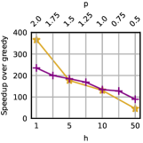
(a) Speedup over the greedy algorithm (geom. mean).

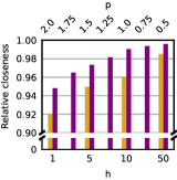
(b) Closeness score relative to the score of the group returned by greedy (geom. mean).

Figure 2: Performance of the extended Grow-Shrink algorithm for different values of $h$ or $p$ on unweighted graphs, $k=10$.

In a first experiment, we evaluate performance of our extended Grow-Shrink algorithm and compare it to the greedy heuristic. Because of its ability to escape local optima, we expect this to be the best algorithm in terms of quality; hence, it should be a good default choice among our algorithms. For this experiment, we set $k=10$.

As discussed in Section II-D4, we distinguish two strategies to determine $h$: we either fix a constant $h$, or we fix a constant $p$. For each strategy, we evaluate multiple values for $h$ or $p$. Results for both strategies are shown in Figure 2. As expected, higher values of $h$ (or, similarly, lower values of $p$) increase the algorithm’s running time; (while $h>1$ allows the algorithm to perform better choices, it does not converge $h$-times as fast). Still, for all tested values of $h$ or $p$, the extended Grow-Shrink algorithm is one to two orders of magnitude faster than the greedy baseline. Furthermore, values of $p<1$ yield results of very good quality: for $p=0.75$, for example, we achieve a quality of $$99.382\,573\,688\,401\,14$\%$. At the same time, using this setting for $p$, our algorithm is $$127.833\,197\,154\,403\,05$\times$ faster than the greedy algorithm. We remark that for all but the smallest values of $h$ (i. e., those corresponding to the lowest quality), choosing constant $p$ is a better strategy than choosing constant $h$: for the same running time, constant $p$ always achieves solutions of higher quality.

III-B Scalability to Large Graphs

We also analyze the running time of our extended Grow-Shrink algorithm on large-scale networks. To this end, we switch to graphs larger than the ones in Table II. We fix $p=0.75$, as Section III-A demonstrated that this setting results in a favorable trade-off between solution quality and running time. The greedy algorithm is not included in this experiment as it requires multiple hours of running time, even for the smallest real-world graphs that we consider in this part. Hence, we also do not compare against its solution quality in this experiment.

III-B1 Results on Synthetic Data

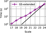
(a) R-MAT networks; $2^{17}$ to $2^{24}$ vertices (up to $268$ million edges).

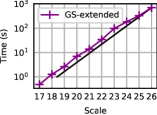
(b) Random hyperbolic networks; $2^{17}$ to $2^{26}$ vertices (up to $671$ million edges).

Figure 3: Running time (s) of the extended Grow-Shrink algorithm on synthetic graphs (black line = linear regression); $p=0.75$, $k=10$.

Figure 3 shows the average running time of our algorithm on randomly generated R-MAT [23] graphs as well as graphs from a generator [24] for random hyperbolic graphs. Like R-MAT, the random hyperbolic model yields graphs with a skewed degree distribution, similar to the one found in real-world complex networks. In the (log-log) plot, the straight lines represent a linear regression of the running times. In both cases, the running time curves are at most as steep as the regression line, i. e., the running time behaves linearly in the number of vertices for the considered network models and sizes.

III-B2 Results on Large Real-World Data Sets

TABLE I: Running time of the extended Grow-Shrink algorithm on large real-world networks; $p=0.75$, $k=10$.

Network	$|V|$	$|E|$	Time (s)
soc-LiveJournal1	4,843,953	42,845,684	95.3
livejournal-links	5,189,808	48,687,945	135.6
orkut-links	3,072,441	117,184,899	199.9
dbpedia-link	18,265,512	126,888,089	368.0
dimacs10-uk-2002	18,459,128	261,556,721	333.1
wikipedia_link_en	13,591,759	334,640,259	680.1

Table I reports the algorithm’s performance on large real-world graphs. In contrast to the greedy algorithm (which would require hours), our extended Grow-Shrink algorithm can handle real-world graphs with hundreds of millions of edges in a few minutes. For the orkut-links network, Bergamini et al. [12] report running times for greedy of 16 hours on their machine; it is the largest instance in their experiments.

III-C Accelerating Performance on Unweighted Graphs

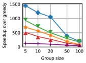
(a) Speedup over the greedy algorithm (geom. mean).

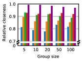
(b) Closeness score relative to the score of the group returned by greedy (geom. mean).

Figure 4: Performance of our local search algorithms for different values of $k$; unweighted graphs.

While the extended Grow-Shrink algorithm yields results of very high quality, if quality is not a primary concern, even faster algorithms might be desirable for very large graphs. To this end, we also evaluate the performance of the non-extended Grow-Shrink and the Local Swap algorithms. For extended Grow-Shrink, we fix $p=0.75$ again. The speedup and the quality of our algorithms over the greedy algorithm, for different values of the group size $k$, is shown in Figures 4(a) and 4(b), respectively. Note that the greedy algorithm scales well to large $k$, so that the speedup of our algorithms decreases with $k$ (as mentioned in Section I, the main bottleneck of greedy is adding the first vertex to the group). However, even for large groups of $k=100$, all of our algorithms are still at least $$42.969\,544\,666\,040\,31$\times$ faster.

After extended Grow-Shrink, our non-extended local version of Grow-Shrink is the next best algorithm in terms of quality. As explained in Section II-D3, this variant yields better solutions than non-local Grow-Shrink and gives a speedup of $$3.134\,114\,991\,269\,074\,2$\times$ over extended Grow-Shrink with $p=0.75$ and $k=10$ (= a speedup of $$365.836\,965\,563\,949\,04$\times$ over greedy); the solution quality in this case is $$92.074\,794\,402\,235\,1$\%$ of the greedy quality.

The non-restricted Local-Swap algorithm is dominated by Grow-Shrink, both regarding running time and solution quality. Furthermore, compared to the other algorithms, the restricted Local-Swap algorithm only gives a rough estimate of the group with highest group closeness; however, it is also significantly faster than all other algorithms and may be employed during an exploratory analysis of graph data sets.

III-D Results on Weighted Road Networks

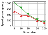
(a) Speedup over the greedy algorithm (geom. mean).

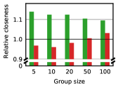
(b) Closeness score relative to the score of the group returned by greedy (geom. mean).

Figure 5: Performance of our local search algorithms for different values of $k$; weighted graphs.

Recall that the Local-Swaps algorithm does not work for weighted graphs; we thus report only Grow-Shrink data in the weighted case. The performance of Grow-Shrink and local Grow-Shrink on weighted graphs is shown in Figure 5. In contrast to unweighted graphs, the quality of the non-local Grow-Shrink algorithm is superior to the greedy baseline for all considered group sizes. Furthermore, in contrast to the unweighted case, the ability to perform non-local vertex exchanges greatly benefits the non-local Grow-Shrink algorithm compared to local Grow-Shrink. Thus, Grow-Shrink clearly dominates both the greedy algorithm and local Grow-Shrink on the weighted graphs in our benchmark set – both in terms of speed and solution quality.

III-E Summary of Experimental Results

On unweighted graphs, a good trade-off between solution quality and running time is achieved by the extended Grow-Shrink algorithm with constant $p=0.75$. This strategy yields solutions with at least $$99.382\,573\,688\,401\,14$\%$ of the closeness score of a greedy solution (greedy, in turn, was at most $3\%$ away from the optimum on small networks in previous work [12]). Extended Grow-Shrink is $$127.833\,197\,154\,403\,05$\times$ faster than greedy ($k=10$). Thus, it is able to handle graphs with hundreds of millions of edges in a few minutes – the state of the art needs multiple hours. If a fast but inaccurate algorithm is needed for exploratory analysis of graph data sets, we recommend to run the non-extended Grow-Shrink algorithm, or, if only a very coarse estimate of the group with maximal closeness is needed, restricted Local-Swap.

On weighted graphs, we recommend to always use our Grow-Shrink algorithm, as it outperforms the greedy state of the art both in terms of quality (yielding solution that are on average $$12.384\,054\,953\,251\,923$\%$ better than greedy solutions) and in terms of running time performance (with a speedup of two orders of magnitude), at the same time.

IV Conclusions

In this paper, we introduced two families of new local-search algorithms for group closeness maximization in large networks. As maximizing group closeness exactly is infeasible for graphs with more than a few thousand edges, our algorithms are heuristics (just like the state-of-the-art greedy algorithm). However, for small real-world networks, the results are empirically known to be close to optimal solutions [12].

Compared to previous state-of-the-art heuristics, our algorithms (in particular: extended Grow-Shrink) allow to find groups with high closeness centrality in real-world networks with hundreds of millions of edges in seconds to minutes instead of multiple hours, while sacrificing less than $1\%$ in quality. In weighted graphs, Grow-Shrink (GS) even dominates the best known heuristic: the GS solution quality is more than $10\%$ higher and GS is two orders of magnitude faster. Adapting the algorithm to even larger graphs in distributed memory is left to future work.

Appendix A Technical Proofs

Proof of Lemma 1.

Let $x\in D_{v}$. Because of the sub path optimality property of shortest paths, it is clear that $\mathrm{dist}(S,x)=\mathrm{dist}(S,v)+\mathrm{dist}(v,x)$ (as $v$ is a predecessor of $x$ on a shortest path from $S$). On the other hand, adding $v$ to $S$ decreases the length of this path (as the distance between $S$ and $v$ becomes zero); in other words: $\mathrm{dist}(S^{+v},x)=\mathrm{dist}(v,x)$. These observations allow us to express the right-hand side of Eq. 1 as $\mathrm{dist}(S,x)-\mathrm{dist}(S^{+v},x)=\mathrm{dist}(S,v)$. Summing this equation for all vertices in $D_{v}$ yields the term $|D_{v}|\cdot\mathrm{dist}(S,v)$ of the lemma. For vertices $x\notin D_{v}$, it holds that $\mathrm{dist}(S,x)-\mathrm{dist}(S^{+v},x)\geq 0$, hence the inequality.

For the statement about the unweighted case, we need to show that the contribution of all other vertices is zero, i. e., $\mathrm{dist}(S,x)=\mathrm{dist}(S^{+v},x)$ for all vertices $x\notin D_{v}$. Note that $\mathrm{dist}(S,x)<\mathrm{dist}(S,v)+\mathrm{dist}(v,x)$ (otherwise $x$ would be in $D_{v}$) and $\mathrm{dist}(S,v)=1$. Thus, $\mathrm{dist}(S,x)\leq\mathrm{dist}(v,x)$ which completes the proof. ∎

Proof of Lemma 4.

Let $Z$ be the set of vertices that need to be updated by the algorithm, i. e., $Z$ equals the set $R_{u}\cup R^{\prime}_{u}$ before the Dijkstra-like algorithm runs. We have not shown yet whether all vertices in $Z$ are indeed updated. For the remainder of this proof, all symbols (such as $r^{\prime}$, $d^{\prime}$ and $R^{\prime}$) refer to the state of our data structures after the algorithm terminates. To prove the lemma, it is sufficient to prove that $Z=\bigcup_{w\in S}(Z\cap R^{\prime}_{w})$ (i. e., that no $r^{\prime}$ remains undefined, or, in other words, $r^{\prime}$ is updated wherever necessary) and that $\mathrm{dist}(S_{-r(x)},x)=\mathrm{dist}(r^{\prime}(x),x)$ for all $x\in Z$ (i. e., that the definition of $r^{\prime}$ is respected).

Let us first prove that $\bigcup_{w\in S}(Z\cap R^{\prime}_{w})=Z$. Let $z\in Z$. There exists a path from every $w\in S$ to $z$ and each such path contained at least one boundary pair $(x,y)$ before the algorithm started. Indeed, there is a boundary pair for the first vertex $y$ on that path that is also in $Z$. Thus, the algorithm sets $r^{\prime}(y)=w$ for some $w\in S$ (i. e., $y\in Z\cap R^{\prime}_{w}$) and propagates the update of $r^{\prime}$ along the path from $w$ to $z$. We have to prove that our pruning condition does not prevent any necessary update along this path. Hence, let $(x,y)$ be a pair of vertices so that the algorithm is pruned before visiting $y$ from $x$. Only the $y\in Z$ case is interesting, as $r^{\prime}$ must already be correct otherwise. Pruning only happens if $r^{\prime}(x)=r(y)$ and therefore $r(x)\neq r(y)$. But in this case, $(x,y)$ was a $d$-boundary pair and the preceding argument shows that $y\in\bigcup_{w\in S}Z\cap R^{\prime}_{w}$.

Now consider the second part of the proof. Let $w\in S$ be any group vertex and let $y\in Z\cap R_{w}$ be any vertex that is updated by the algorithm with $r(y)=w$. The algorithm guarantees that $\mathrm{dist}(S_{-w},y)\leq\mathrm{dist}(r^{\prime}(y),y)\leq d^{\prime}(y)$ as $r^{\prime}(y)\in S_{-w}$ and (by construction of the algorithm) $d^{\prime}$ is the length of a (not yet proven to be shortest) path from $r^{\prime}(y)$ to $y$. It is sufficient to show that this path is a shortest one, i. e., $\mathrm{dist}(S_{-w},y)=d^{\prime}(y)$. We prove this statement for all $y\in R_{w}$ by an inductive argument using $\mathrm{dist}(S_{-w},y)$. We distinguish two cases depending on whether there exists a neighbor of $y$ in $R_{w}$ that is on a shortest path from $S_{-w}$ to $y$. First, we handle the case that no such neighbor exists. In this case, $r(x)\neq w$ holds for all $x\in N(y)$ on shortest paths from $S_{-w}$ to $y$. As $r(x)$ did not change during the algorithm, all such $x$ correspond to $d$-boundary pairs for $y$ and $\mathrm{dist}(S_{-w},y)$ is the minimal boundary distance over all these pairs $(x,y)$. Hence, $d^{\prime}(y)$ was updated correctly before the Dijkstra-like algorithm ran. On the other hand, let $x\in N(y)\cap R_{w}$ be a neighbor of $y$ that is on a shortest path from $S_{-w}$ to $y$. $x\in R_{w}$ implies $r^{\prime}(x)\neq w$; thus, the algorithm cannot be pruned when visiting $y$ from $x$. In this case, however, the algorithm sets $d^{\prime}(y)=d^{\prime}(x)+\mathrm{dist}(x,y)$. As $\mathrm{dist}(S_{-w},x)<\mathrm{dist}(S_{-w},y)$, the induction yields that $d^{\prime}(x)$ is already correct, i. e., $d^{\prime}(x)=\mathrm{dist}(S_{-w},x)$. Since $x$ is on a shortest path from $S_{-w}$ to $y$, $d^{\prime}(y)$ is also updated correctly. ∎

Appendix B Details of the Experimental Setup

TABLE II: Unweighted real-world networks used in the experiments.

Network	$|V|$	$|E|$	Category
dimacs9-NY	264,346	365,050	Road
dimacs9-BAY	321,270	397,415	Road
web-Stanford	255,265	1,941,926	Hyperlink
hyves	1,402,673	2,777,419	Social
youtube-links	1,134,885	2,987,468	Social
com-youtube	1,134,890	2,987,624	Social
web-Google	855,802	4,291,352	Hyperlink
trec-wt10g	1,458,316	6,225,033	Hyperlink
dimacs10-eu-2005	862,664	16,138,468	Road
soc-pokec-relationships	1,632,803	22,301,964	Social
wikipedia_link_ca	926,588	27,133,794	Hyperlink

TABLE III: Weighted networks used in the experiments. All networks are road networks of different states of the US.

State	$|V|$	$|E|$
DC	9,522	14,807
HI	21,774	26,007
AK	48,560	55,014
DE	48,812	59,502
RI	51,642	66,650
CT	152,036	184,393
ME	187,315	206,176

State	$|V|$	$|E|$
ND	203,583	249,809
SD	206,998	249,828
WY	243,545	293,825
ID	265,552	310,684
MD	264,378	312,977
WV	292,557	320,708
NE	304,335	380,004

Tables II and  III show details about our real-world instances. To generate the synthetic graphs in Figure 3, we use the same parameter setting as in the Graph 500’s benchmark [25] (i. e., edge factor 16, $a=0.57$, $b=0.19$, $c=0.19$, and $d=0.05$) for the R-MAT generator. For the random hyperbolic generator, we set the average degree to $20$, and the exponent of the power-law distribution to 3.

Appendix C Additional Experiments

C-A Impact of the number of vertex exchanges

Figures 7(a) and 7(b) depict the relative closeness (compared to the closeness of the group returned by the greedy algorithm), depending on the progress of the algorithm in terms of vertex exchanges. For extended Grow-Shrink, we fix $p=0.75$. All of the local search algorithm quickly converge to a value near their final result; additional vertex exchanges improve the group closeness score by small amounts. In order to avoid an excessive amount of iterations, it seems reasonable to set a limit on the number of vertex exchanges. In our experiments we set a conservative limit of 100 exchanges.

C-B Impact of reachability set size approximation

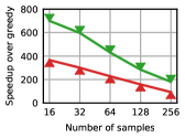
(a) Speedup over the greedy algorithm (geom. mean).

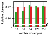
(b) Closeness score relative to the score of the group returned by greedy (geom. mean).

Figure 6: Performance of the Grow-Shrink algorithm for different numbers of samples to estimate reachability set size; $k=10$.

As mentioned in Section II-D3, the errors in the approximation of $|D_{v}|$ are amplified by the multiplication with $\mathrm{dist}(S,v)$, and this results in GS-local computing higher quality solutions than GS. We study how increasing the accuracy of the reachability set size approximation by incrementing the number of samples impacts the performances of both GS and GS-local. Figure 6(a) shows that GS needs at least 64 samples to converge to a better local optimum than GS-local. However, in both cases increasing the number of samples degrades the speedup without yielding a significant quality improvement (Figure 6(b)).

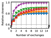
(a) Unweighted graphs.

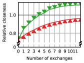
(b) Weighted graphs.

Figure 7: Behavior of the relative closeness score (compared to the group returned by greedy, geom. mean) over the execution of the algorithms (in terms of vertex exchanges); $k=10$.

References

- [1] M. Newman, Networks, 2nd ed. Oxford university press, 2018.
- [2] P. Boldi and S. Vigna, “Axioms for centrality,” Internet Mathematics, vol. 10, no. 3-4, pp. 222–262, 2014.
- [3] A. Bavelas, “A mathematical model for group structures,” Human organization, vol. 7, no. 3, p. 16, 1948.
- [4] E. Bergamini, M. Borassi, P. Crescenzi, A. Marino, and H. Meyerhenke, “Computing top-k closeness centrality faster in unweighted graphs,” ACM Transactions on Knowledge Discovery from Data (TKDD), vol. 13, no. 5, p. 53, 2019.
- [5] K. Okamoto, W. Chen, and X.-Y. Li, “Ranking of closeness centrality for large-scale social networks,” in International Workshop on Frontiers in Algorithmics. Springer, 2008, pp. 186–195.
- [6] P. W. Olsen, A. G. Labouseur, and J.-H. Hwang, “Efficient top-k closeness centrality search,” in 2014 IEEE 30th International Conference on Data Engineering. IEEE, 2014, pp. 196–207.
- [7] C. Chen, W. Wang, and X. Wang, “Efficient maximum closeness centrality group identification,” in Australasian Database Conference. Springer, 2016, pp. 43–55.
- [8] T. Zhu, B. Wang, B. Wu, and C. Zhu, “Maximizing the spread of influence ranking in social networks,” Information Sciences, vol. 278, pp. 535–544, 2014.
- [9] C. Gkantsidis, M. Mihail, and A. Saberi, “Random walks in peer-to-peer networks,” in IEEE INFOCOM 2004, vol. 1. IEEE, 2004.
- [10] L. Leydesdorff, “Betweenness centrality as an indicator of the interdisciplinarity of scientific journals,” Journal of the American Society for Information Science and Technology, vol. 58, no. 9, pp. 1303–1319, 2007.
- [11] M. G. Everett and S. P. Borgatti, “The centrality of groups and classes,” The Journal of mathematical sociology, vol. 23, no. 3, pp. 181–201, 1999.
- [12] E. Bergamini, T. Gonser, and H. Meyerhenke, “Scaling up group closeness maximization,” in 2018 Proceedings of the Twentieth Workshop on Algorithm Engineering and Experiments (ALENEX). SIAM, 2018, pp. 209–222.
- [13] ——, “Scaling up group closeness maximization,” CoRR, vol. abs/1710.01144, 2017, updated on May 15, 2019. [Online]. Available: http://arxiv.org/abs/1710.01144
- [14] F. Le Gall, “Powers of tensors and fast matrix multiplication,” in Proceedings of the 39th international symposium on symbolic and algebraic computation. ACM, 2014, pp. 296–303.
- [15] E. Cohen, “Size-estimation framework with applications to transitive closure and reachability,” Journal of Computer and System Sciences, vol. 55, no. 3, pp. 441–453, 1997.
- [16] D. A. Bader, G. Cong, and J. Feo, “On the architectural requirements for efficient execution of graph algorithms,” in Parallel Processing, 2005. ICPP 2005. International Conference on. IEEE, 2005, pp. 547–556.
- [17] A. Lumsdaine, D. Gregor, B. Hendrickson, and J. Berry, “Challenges in parallel graph processing,” Parallel Processing Letters, vol. 17, no. 01, pp. 5–20, 2007.
- [18] C. Demetrescu, A. V. Goldberg, and D. S. Johnson, The Shortest Path Problem: Ninth DIMACS Implementation Challenge. American Mathematical Soc., 2009, vol. 74.
- [19] J. Kunegis, “Konect: the Koblenz Network Collection,” in Proceedings of the 22nd International Conference on World Wide Web. ACM, 2013, pp. 1343–1350.
- [20] C. L. Staudt, A. Sazonovs, and H. Meyerhenke, “Networkit: A tool suite for large-scale complex network analysis,” Network Science, vol. 4, no. 4, pp. 508–530, 2016.
- [21] M. E. O’Neill, “Pcg: A family of simple fast space-efficient statistically good algorithms for random number generation,” Harvey Mudd College, Claremont, CA, Tech. Rep. HMC-CS-2014-0905, Sep. 2014.
- [22] E. Angriman, A. v. d. Grinten, M. v. Looz, H. Meyerhenke, M. Nöllenburg, M. Predari, and C. Tzovas, “Guidelines for experimental algorithmics: A case study in network analysis,” Algorithms, vol. 12, no. 7, p. 127, 2019.
- [23] D. Chakrabarti, Y. Zhan, and C. Faloutsos, “R-mat: A recursive model for graph mining,” in Proceedings of the 2004 SIAM International Conference on Data Mining. SIAM, 2004, pp. 442–446.
- [24] M. von Looz, M. S. Özdayi, S. Laue, and H. Meyerhenke, “Generating massive complex networks with hyperbolic geometry faster in practice,” in 2016 IEEE High Performance Extreme Computing Conference (HPEC). IEEE, 2016, pp. 1–6.
- [25] R. C. Murphy, K. B. Wheeler, B. W. Barrett, and J. A. Ang, “Introducing the graph 500,” Cray Users Group (CUG), vol. 19, pp. 45–74, 2010.