GMC Collisions as Triggers of Star Formation. VII.
The Effect of Magnetic Field Strength on Star Formation

Abstract

We investigate the formation of stars within giant molecular clouds (GMCs) evolving in environments of different global magnetic field strength and large-scale dynamics. Building upon a series of magnetohydrodynamic (MHD) simulations of non-colliding and colliding GMCs, we employ density- and magnetically-regulated star formation sub-grid models in clouds which range from moderately magnetically supercritical to near critical. We examine gas and star cluster morphologies, magnetic field strengths and relative orientations, pre-stellar core densities, temperatures, mass-to-flux ratios and velocities, star formation rates and efficiencies over time, spatial clustering of stars, and kinematics of the stars and natal gas. The large scale magnetic criticality of the region greatly affects the overall gas evolution and star formation properties. GMC collisions enhance star formation rates and efficiencies in magnetically supercritical conditions, but may actually inhibit them in the magnetically critical case. This may have implications for star formation in different Galactic environments such as the Galactic Center and the main Galactic disk.

1 Introduction

Giant molecular cloud (GMC) collisions have been posited as a mechanism for triggering the formation of stars and possibly even setting global star formation rates (SFRs) in disk galaxies (e.g., Scoville et al., 1986; Tan, 2000). Such converging molecular flows are likely to form regions of dense, gravitationally unstable gas with properties similar to those observed in Infrared Dark Clouds (IRDCs; see e.g., Tan et al., 2014).

On the other hand, magnetic fields ($B$-fields) in the interstellar medium (ISM) may act as an important regulator of star formation in GMCs, as studies have found reductions of overall fragmentation, SFRs, and star formation efficiency (SFE) by factors of a few upon the inclusion of $B$-fields in driven turbulence simulations (see, e.g., Padoan & Nordlund, 2011; Federrath & Klessen, 2012). $B$-fields in conjunction with turbulence may help explain the very inefficient SFRs per local free-fall time observed on average within GMCs (Zuckerman & Evans, 1974; Krumholz & Tan, 2007), as thermal pressures are relatively insignificant at the $T\sim 10-20\>$K temperatures within GMCs. Such regulating mechanisms alone, however, may be unable to explain the high variation in observed SFRs (Lee et al., 2016). Here, irregular, intermittent phenomena such as GMC collisions may play a key role.

the frequency of cloud-cloud interactions has been difficult to determine. Earlier studies estimated timescales of order 100 Myr between collisions, casting doubt on the prevalence of this mechanism (Blitz & Shu, 1980). However, upon accounting for self-gravity, differential rotation, and an effectively 2D geometry due to disk scale height constraints, predicted cloud collision timescales are reduced significantly (Gammie et al., 1991; Tan, 2000). Global galaxy simulations by, e.g., Tasker & Tan (2009); Dobbs et al. (2015); Fujimoto et al. (2014); Li et al. (2018) showed that, on average, a molecular cloud experiences a collision every $\sim 1/5$ of a local galactic orbit (i.e., every $\sim$20 Myr at a galactocentric radius of $\sim 4\>$kpc in the Milky Way), with even shorter timescales possible for the most massive clouds and in the presence of spiral and bar potentials.

A growing number of observations of dense clumps and young massive clusters have claimed evidence of cloud-cloud collisions (e.g., Loren, 1976; Furukawa et al., 2009; Torii et al., 2011; Nakamura et al., 2012; Sanhueza et al., 2013; Fukui et al., 2014; Nishimura et al., 2018; Dobashi et al., 2019). Disrupted gas morphology, multiple velocity components, proximity to young massive stars, broad bridge features in position-velocity space, and molecular and atomic kinematic tracers are all diagnostics predicted to differentiate GMC collisions from non-colliding clouds. Frequently, however, the complexity of the blue and redshifted velocity fields and the ambiguity of observational features cannot rule out alternative explanations, such as internal gas motions or coincidental projection effects.

Nevertheless, the nature of typical cloud collisions, their outcomes, and definitive ways to distinguish them are all still unanswered questions. The current work continues a series of papers that has been methodically studying the nature of GMC-GMC collisions within a magnetized ISM. Papers I (Wu et al., 2015) and II (Wu et al., 2017b) performed parameter space explorations and laid the numerical framework in 2D and 3D, respectively, of ideal magnetohydrodynamics (MHD), gas heating/cooling, and turbulence. Paper III (Wu et al., 2017a) implemented star formation in the form of two sub-grid models: density regulated and magnetically regulated. Paper IV (Christie et al., 2017) implemented the non-ideal MHD effects of ambipolar diffusion, Paper V (Bisbas et al., 2017) examined observational signatures using radiative transfer post-processing, and Paper VI (Wu et al., 2018) studied collision-induced turbulence.

In this paper, we investigate how the strength of the magnetic field affects the nature of star formation in non-colliding and colliding GMCs. We aim to expand our understanding of how star formation proceeds in different galactic environments, where $10^{5}\>M_{\odot}$, $r\sim 1$pc clouds can be observed to be mostly starless (e.g., in the Galactic Center) or forming massive young clusters (e.g., in the disk) (see, e.g., Longmore et al., 2014; Tan et al., 2014; Sanhueza et al., 2019).

Our numerical set-up is presented in §2. §3 details the results, which include cloud and cluster morphologies, magnetic field orientations and strengths, probability distribution functions (PDFs), properties of star-forming gas, star formation rates and efficiencies, spatial clustering, and star versus gas kinematics. Finally, conclusions are discussed in §4.

2 Numerical Model

2.1 Initial Conditions

Our numerical simulations are based on the GMC models introduced in Paper II with star-formation routines introduced in Paper III and a number of numerical improvements from Paper IV. Specifically, we include heating/cooling, self-gravity, supersonic turbulence, ideal MHD, and investigate both density and magnetically-regulated star formation. In this work, our main goal is to explore the effects of varying magnetic field strengths at the global GMC scale. This, in turn, affects the star formation routines at the sub-grid scale. The physical properties of our models are summarized in Table 1 and detailed below.

Within a simulation cube of side length $L=128\>{\rm pc}$, two identical GMCs are initialized as uniform spheres with radii $R_{\rm GMC}=20.0$ pc and Hydrogen number densities $n_{\rm H,GMC}=100\>{\rm cm^{-3}}$, giving masses of $M_{\rm GMC}=9.3\times 10^{4}\>M_{\odot}$. The GMC centers are offset by an impact parameter $b=0.5R_{\rm GMC}$. The clouds are embedded within ambient gas of ten times lower density $n_{\rm H,0}=10\>{\rm cm^{-3}}$, filling the remainder of the volume and representative of an atomic cold neutral medium (CNM). In the non-colliding model, there is no additional bulk velocity field, while in the colliding model, both the CNM and GMCs are converging with a relative velocity of $v_{\rm rel}=10\>{\rm km\>s^{-1}}$ along the collision axis (defined as the $x$-axis). This collision velocity is consistent with the peak of the distribution of relative velocities from interacting GMCs tracked in global galactic simulations (e.g., Li et al., 2018).

A uniform magnetic field is initialized throughout the entire domain at an angle $\theta=60^{\circ}$ with respect to the collision axis. To investigate the role of magnetic strength on gas dynamics and star formation, we initialize fields with magnitudes of $B=10,30,$ and $50\>{\rm\mu G}$, which correspond to configurations of GMCs with average dimensionless mass-to-flux ratios $\lambda_{\rm GMC}=(M/\Phi)(\sqrt{G}/0.126)$ = 5.4 (i.e., moderately magnetically supercritical), 1.8 (i.e., marginally supercritical), and 1.1 (i.e., near critical), respectively. Note that due to the spherical geometry, there are much larger columns through the cloud centers, resulting in higher degrees of supercriticality in central flux tubes and lower degrees near cloud boundaries. The equilibrium temperature of molecular gas within the GMCs is $\sim 15$ K, which yields thermal-to-magnetic pressure ratios $\beta=8\pi c_{s}^{2}\rho/B^{2}=1.5\times 10^{-2}$, $1.6\times 10^{-3}$, and $6.0\times 10^{-4}$, respectively. While $B\sim 10\>{\rm\mu G}$ has been inferred from Zeeman measurements of nearby GMCs, as summarized by Crutcher (2012), much stronger magnetic fields of order have been estimated to be present in IRDCs (e.g., Pillai et al., 2015, 2016; Liu et al., 2018b; Soam et al., 2019).

We approximate the complex density and velocity structures observed in GMCs by initializing gas within our model clouds with a solenoidal random supersonic turbulent velocity field. The clouds are of order virial, with Mach number $\mathcal{M}_{s}\equiv\sigma/c_{s}=23$ (for $T=15$ K). The velocity field follows a $v_{k}^{2}\propto k^{-4}$ relation, where $k$ is the wavenumber and each $k$-mode spanning $2<k/(\pi/L)<20$ is excited. We do not drive turbulence, but rather let it decay. Note, however, that GMC collisions themselves provide an additional mode of turbulence driving (Wu et al., 2018).

As in Paper III, the simulations are run for $5\>{\rm Myr}$ to investigate the initial phases of star formation in both non-colliding and colliding cases. For reference, the freefall time for the initial uniform density GMCs is $t_{\rm ff}=(3\pi/[32G\rho])^{1/2}=4.35$ Myr, but the values of the local $t_{\rm ff}$ for denser substructures formed from turbulence and the collision are much shorter.

Table 1: Initial Simulation Properties

Gas Properties		GMC	Ambient
$n_{\rm H}$	(${\rm cm}^{-3}$)	100	10
$R$	(${\rm pc}$)	20	-
$M$	($M_{\odot}$)	$9.3\times 10^{4}$	-
$t_{\rm ff}$	(Myr)	4.35	13.8
$T$	(K)	15	150
$c_{\rm s}$	(km/s)	0.23	0.72
$v_{\rm vir}$	(km/s)	4.9	-
$v_{\rm bulk}$	(km/s)	[0; $\pm 5$]
Turbulence Properties
$k$-mode	($\pi/L$)	$\{k_{1}=2,k_{2}=20\}$	-
$\sigma$	(km/s)	5.2	-
$\mathcal{M}_{\rm s}$		23	-
Magnetic Field Properties
$B$	(${\rm\mu G}$)	(10, 30, 50)
$\beta$		($1.5\times 10^{-2}$, $1.7\times 10^{-3}$, $6.0\times 10^{-4}$)
$\lambda$		(5.8, 1.8, 1.1)	(1.9, 0.6, 0.4)
$v_{A}$	(km/s)	(1.84, 5.52, 9.2)	(5.83, 17.49, 29.2)
$\mathcal{M}_{A}$		(2.82, 0.94, 0.57)	-

2.2 Numerical Code

The magnetohydrodynamics (MHD) adaptive mesh refinement (AMR) code Enzo (Bryan et al., 2014) is used to run our simulations, specifically utilizing the Dedner MHD solver and hyperbolic divergence cleaning method (Dedner et al., 2002; Wang & Abel, 2008). We use a root grid of $128^{3}$ with 3 additional levels of AMR, resulting in an effective resolution of $1024^{3}$ and minimum grid cell size of 0.125 pc. While our refinement criterion is based on resolving the Jeans length by 8 cells (see, e.g., Truelove et al., 1997), this means that finer grid cells are placed everywhere in the GMC regions and Jeans fragmentation is not well resolved at densities where the Jeans length becomes $\lesssim 1\>$pc (i.e., $n_{\rm H}\gtrsim 2.1\times 10^{2}\>{\rm cm^{-3}}$). However, note that the Jeans criterion assumes purely thermal support, so the effective “magneto-Jeans length” of magnetized gas will be significantly larger perpendicular to the magnetic field, so magnetically-regulated fragmentation will be better resolved. Still, it is not our goal in this paper to accurately follow the fragmentation of very dense gas structures, e.g., that may be relevant to the core mass function, but rather the overall efficiency of dense gas formation and more global aspects of its morphology.

Heating and cooling are governed by functions based on modeling of photo-dissociation regions (PDRs; see Wu et al., 2015) and implemented via the Grackle 2.2 chemistry library (Smith et al., 2017). We additionally utilize: the “dual energy formalism” (Bryan et al., 2014), important for accurate calculations of pressures and temperatures in conditions of low thermal-to-total energy ratios (e.g., in the presence of relatively high bulk velocities and strong magnetic fields); an “Alfvén limiter” (described in Paper II) to avoid extremely short timesteps set by Alfvén waves by choosing a maximum Alfvén velocity, $v_{A,{\rm max}}=B/\sqrt{4\pi\rho_{\rm min}}=1\times 10^{7}\>{\rm cm\>s^{-1}}$; and a minimum cooling timestep (described in Paper IV) of $t_{\rm cool,min}\sim 600$ yr to avoid prohibitively short timesteps at high densities.

2.3 Star Formation Models

The star formation process is represented by the density-regulated and magnetically-regulated sub-grid star formation routines introduced in Paper III. For both star formation models, star particles (i.e., collisionless, point particles with mass $m_{\star}$) form within a simulation cell if the following criteria are met. First, the cell must be at the finest level of resolution, determined by the local Jeans length. Second, the temperature in the cell must be $<3000$ K to prevent stars from forming in transient shock-heated dense regions. Third, the cell must exceed certain physical thresholds. In the density-regulated model, a constant density threshold of $n_{\rm H,sf}=1.0\times 10^{6}\>{\rm cm}^{-3}$ is required. In the magnetically-regulated model, the cell must be locally magnetically “supercritical” (i.e., having a mass-to-flux ratio $\mu_{\rm cell}>1$). The dimensionless mass-to-flux ratio is

$$\mu_{\rm cell}=\frac{\rho\Delta x\sqrt{G}}{Bc_{1}}$$ (1)

for a cell of edge length $\Delta x$, gas density $\rho$, magnetic field strength $B$, and using gravitational constant $G$. The value of $c_{1}$ depends on the extended geometry of the flux tube, which we set to be $c_{\rm 1,fid}=0.126$ (for an isolated cloud, Mouschovias & Spitzer, 1976). See also Nakano & Nakamura (1978) for an infinite disk, in which case $c_{1}=\frac{1}{2\pi}\sim 0.159$. We explore variations in this threshold of a factor of two higher and lower for the magnetically-regulated model.

The resulting expression for star-formation threshold density as a function of magnetic field strength can then be written as

$$n_{\rm H} > \frac{Bc_{1}}{\mu_{\rm H}m_{\rm H}\Delta x\sqrt{G}}$$ (2)

$$= 5.42\times 10^{3}\left(\frac{B}{10\>{\rm\mu G}}\right)\left(\frac{c_{1}}{0.126}\right)\left(\frac{\Delta x}{0.125\>{\rm pc}}\right)^{-1}{\rm cm}^{-3},$$ (3)

where the mean particle mass per hydrogen is $\mu_{\rm H}m_{\rm H}=1.4m_{\rm H}$.

Finally, if the required thresholds for a given model are satisfied, a fraction of the gas mass in the cell is transformed into star particles such that the average rate follows a fixed star formation efficiency per local free-fall time, $\epsilon_{\rm ff}=0.02$. The local free-fall time, $t_{\rm ff}$, approximated as the collapse of a uniform density sphere, is

$$t_{\rm ff} = \left(\frac{3\pi}{32G\rho}\right)^{1/2}$$ (4)

$$= 4.4\times 10^{4}n_{\rm H,6}^{-1/2}\>{\rm yr},$$ (5)

where $n_{\rm H,6}\equiv n_{\rm H}/10^{6}\>{\rm cm^{-3}}$. This results in a SFR of

$$\dot{m}_{\star} = \epsilon_{\rm ff}\frac{m_{\rm gas}}{t_{\rm ff}}$$ (6)

$$= 2.9\times 10^{-5}\left(\frac{\epsilon_{\rm ff}}{0.02}\right)\left(\frac{\Delta x}{0.125\>{\rm pc}}\right)^{3}n_{\rm H,6}^{3/2}\>M_{\odot}\>{\rm yr}^{-1}.$$ (7)

Table 2: List of Simulations

Name	Star Formation	$v_{\rm rel}$	$B$	$\Delta x$	$n_{\rm H,sf}$	$t_{\rm ff}$	$m_{\rm gas,min}$	$m_{\rm\star,min}$	$c_{1}$
	Model	(${\rm km\>s^{-1}}$)	($\mu$G)	(pc)	(cm-3)	(years)	($M_{\odot}$)	($M_{\odot}$)	($c_{\rm 1,fid}$)
B10-d1-nocol	density	0	10	0.125	$1.0\times 10^{6}$	$4.4\times 10^{4}$	6.3	1	…
B10-05-nocol	magnetic	0	10	0.125	$3.55\times 10^{4}$	$2.3\times 10^{5}$	2	1	$0.5$
B10-1-nocol	magnetic	0	10	0.125	$3.55\times 10^{4}$	$2.3\times 10^{5}$	2	1	$1.0$
B10-2-nocol	magnetic	0	10	0.125	$3.55\times 10^{4}$	$2.3\times 10^{5}$	2	1	$2.0$
B30-d1-nocol	density	0	30	0.125	$1.0\times 10^{6}$	$4.4\times 10^{4}$	6.3	1	…
B30-05-nocol	magnetic	0	30	0.125	$3.55\times 10^{4}$	$2.3\times 10^{5}$	2	1	$0.5$
B30-1-nocol	magnetic	0	30	0.125	$3.55\times 10^{4}$	$2.3\times 10^{5}$	2	1	$1.0$
B30-2-nocol	magnetic	0	30	0.125	$3.55\times 10^{4}$	$2.3\times 10^{5}$	2	1	$2.0$
B50-d1-nocol	density	0	50	0.125	$1.0\times 10^{6}$	$4.4\times 10^{4}$	6.3	1	…
B50-05-nocol	magnetic	0	50	0.125	$3.55\times 10^{4}$	$2.3\times 10^{5}$	2	1	$0.5$
B50-1-nocol	magnetic	0	50	0.125	$3.55\times 10^{4}$	$2.3\times 10^{5}$	2	1	$1.0$
B50-2-nocol	magnetic	0	50	0.125	$3.55\times 10^{4}$	$2.3\times 10^{5}$	2	1	$2.0$
B10-d1-col	density	10	10	0.125	$1.0\times 10^{6}$	$4.4\times 10^{4}$	6.3	1	…
B10-05-col	magnetic	10	10	0.125	$3.55\times 10^{4}$	$2.3\times 10^{5}$	2	1	$0.5$
B10-1-col	magnetic	10	10	0.125	$3.55\times 10^{4}$	$2.3\times 10^{5}$	2	1	$1.0$
B10-2-col	magnetic	10	10	0.125	$3.55\times 10^{4}$	$2.3\times 10^{5}$	2	1	$2.0$
B30-d1-col	density	10	30	0.125	$1.0\times 10^{6}$	$4.4\times 10^{4}$	6.3	1	…
B30-05-col	magnetic	10	30	0.125	$3.55\times 10^{4}$	$2.3\times 10^{5}$	2	1	$0.5$
B30-1-col	magnetic	10	30	0.125	$3.55\times 10^{4}$	$2.3\times 10^{5}$	2	1	$1.0$
B30-2-col	magnetic	10	30	0.125	$3.55\times 10^{4}$	$2.3\times 10^{5}$	2	1	$2.0$
B50-d1-col	density	10	50	0.125	$1.0\times 10^{6}$	$4.4\times 10^{4}$	6.3	1	…
B50-05-col	magnetic	10	50	0.125	$3.55\times 10^{4}$	$2.3\times 10^{5}$	2	1	$0.5$
B50-1-col	magnetic	10	50	0.125	$3.55\times 10^{4}$	$2.3\times 10^{5}$	2	1	$1.0$
B50-2-col	magnetic	10	50	0.125	$3.55\times 10^{4}$	$2.3\times 10^{5}$	2	1	$2.0$

As our simulation timesteps are much shorter than the sound crossing time for a cell (i.e., $\ll 1.2\times 10^{5}$ yr for a $1\>{\rm km\>s^{-1}}$ signal speed), the rates defined above typically lead to small expected stellar masses ($\lesssim 1\>M_{\odot}$). However, to avoid excessively large numbers of star particles we adopt a minimum star particle mass, $m_{\rm\star,min}=1\>M_{\odot}$. If the stellar mass expected to be formed in a cell is $m_{\rm\star}<1\>M_{\odot}$, its formation is treated stochastically. In this “stochastic regime”, a $1\>M_{\odot}$ star particle is created with a probability $\dot{m}_{\star}\Delta t/m_{\rm\star,min}$, where $\Delta t$ is the simulation timestep. However, for cases where $\dot{m}_{\star}\Delta t>m_{\rm\star,min}$, a star particle with this mass is simply formed and it is possible for a distribution of initial stellar masses to be created. However, we caution that with such a simple model we do not expect this distribution to necessarily have any similarity to that of the actual stellar initial mass function (IMF).

Note that we limit the fraction of gas mass in a cell that can turn into stars within a single timestep to $<0.5$. In conjunction with the minimum star particle mass, this imposes an effective density threshold on the cell of $n_{\rm H,sf}=3.55\times 10^{4}\>{\rm cm^{-3}}$. This threshold plays a role in the magnetically-regulated SF routine but is superseded by the standard density threshold of the density-regulated SF routine.

3 Results

Overall, we compare the results of 24 different simulations. For both non-colliding (“nocol”) and colliding (“col”) GMC cases, magnetic field strengths of 10, 30, and 50$\mu$G are initialized, respectively. For each of these cases, one density regulated and three magnetically regulated SF models ($c_{1}$=0.5, 1.0, and 2.0 $c_{\rm 1,fid}$) are run. The star formation and physical parameters used each simulation are listed in Table 2.

We analyze various aspects of star formation activity among the collection of non-colliding and colliding simulations at different magnetic field strengths. In particular, we discuss: morphology of the clouds and clusters (§3.1); magnetic field orientations and strengths (§3.2); probability distribution functions (§3.3); properties of star-forming gas (§3.4); global star formation rates (§3.5); spatial clustering of stars (§3.6); and star versus gas kinematics (§3.7).

In most visualizations, we use the $(x,y,z)$ coordinate system as defined in the simulations. Occasionally, we use $(x^{\prime},y^{\prime},z^{\prime})$, where the axes are rotated by the polar and azimuthal angles $(\theta,\phi)=(15^{\circ},15^{\circ})$ when appropriate (e.g., representing certain observables).

3.1 Cloud and Cluster Morphologies

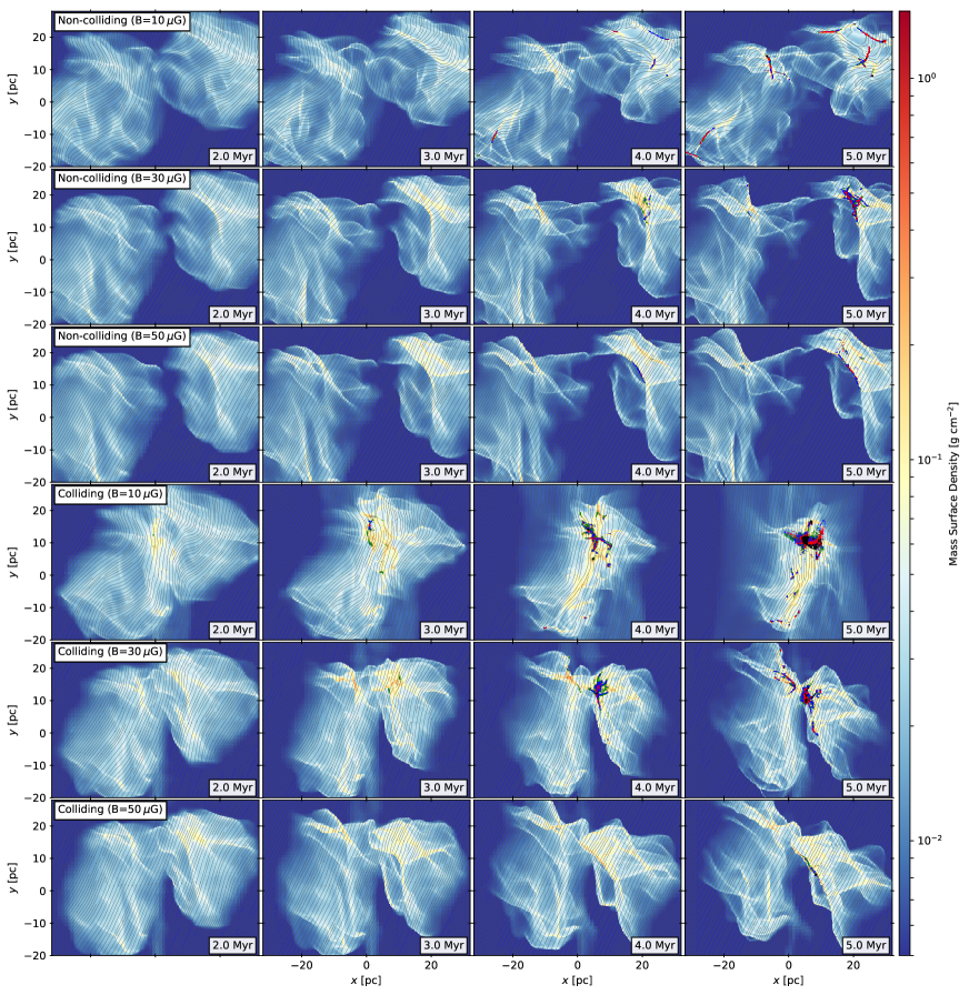
Figure 1: Time evolution of gas mass surface density, magnetic fields, and stellar distributions for all models with density regulated SF. Snapshots at 2.0, 3.0, 4.0, and 5.0 Myr (left to right) are shown projected along the $z$-axis. The top three rows display the non-colliding runs with $B=$10, 30 and 50$\mu$G, respectively, while the bottom three rows display the colliding runs with $B=$10, 30 and 50$\mu$G, respectively. Density-weighted projected magnetic fields are shown as gray streamlines. The corresponding star particles are shown as black points. Stars created in simulations using the star formation models with $c_{1}=0.5c_{\rm 1,fid}$, $1.0c_{\rm 1,fid}$, and $2.0c_{\rm 1,fid}$ are additionally plotted as blue, green, and red points, respectively.

Gas and star particle distribution morphologies for the complete set of simulations are shown in Figure 1. The time evolution of gas mass surface density and star particle distributions for $B=$10, 30, and 50$\mu$G are displayed for each non-colliding and colliding case where $c_{1}=c_{\rm 1,fid}$. Star positions from each of the SF models are additionally plotted as separate colors. This was chosen to more clearly compare the resulting star cluster distribution, as the gas morphology does not differ significantly for a given model based on our chosen SF model $c_{1}$ (cf., Wu et al., 2017a).

In general, the gas in non-colliding GMCs forms more dispersed networks of filaments in contrast to the compressed structures arising in colliding GMCs. The collision also enhances the mass surface densities in both the filamentary gas and ambient material by factors of a few or more. This enhancement occurs at earlier evolutionary times relative to the non-colliding cases, due to the additional accumulation of gas from the colliding flows.

The star clusters that form in each case are also morphologically distinct, with the non-colliding clouds exhibiting more isolated clusters elongated along the densest filaments while the colliding clouds create one primary central cluster with smaller groupings forming in dense knots within the central filamentary clump. The density-regulated SF model forms clusters that span the smallest extent, often at nodes where filaments intersect. As $c_{1}$ decreases for the magnetically-regulated models, the magnetic criticality threshold for star formation to occur is relaxed, increasing the physical elongation of the star clusters and overall number of cluster members along filamentary regions.

For non-colliding GMCs, the strength of the initial $B$-field moderately influences the overall morphology. Self-gravity and turbulence form distributed networks of filaments which gradually increase in mass surface density. For weaker overall $B$-fields, the gas fragments and collapses more readily, resulting in more numerous and physically separated filaments. Stronger $B$-fields tend to create smoother, more connected filamentary structures. In the weaker field case the projected magnetic field has much greater curvature, while in the stronger field case it is less perturbed from the initial configuration. The star formation behavior is notably affected by the $B$-field strength. With weaker fields, elongated star clusters are spread throughout the greater GMC complex. For the 30 and 50$\mu$G cases, star formation becomes concentrated in a single high density region. The density-regulated SF model does not form stars in the latter case.

The strength of the $B$-field significantly affects the evolution of the colliding GMC models. In the weaker field case, both GMCs and $B$-fields are strongly compressed in the central colliding region, forming a large dense filament aligned perpendicular to the collision axis with $B$-fields generally reoriented parallel to this filament at large scales. For stronger field cases, the anisotropy of the magnetic pressure causes the collision to become less direct. Gas is still compressed in the colliding region, but the $B$-fields play a more dominant role, preferentially guiding gas along the field lines. These combined effects result in dense filaments that form within the colliding region, which become qualitatively more perpendicular to the mean field direction as the field strength increases. Star cluster formation occurs within these dense regions. In our models, the surrounding low density CNM contains higher magnetic pressure and effectively creates a barrier inhibiting direct merging of gas between the two GMCs, especially in the 50$\mu$G case. This may indicate that GMC interactions in higher $B$-field environments are more indirect in nature or may preferentially occur along field lines.

3.2 Magnetic Field Orientations and Strengths

The role of $B$-fields in star formation is closely tied with how they influence molecular cloud gas evolution. In super-Alfvénic regimes (i.e., $B$-fields are weak relative to kinetic motions), gas flows dominate the morphology of the $B$-field, yet increase the field strength along compressed regions. In sub-Alfvénic regimes (i.e., $B$-fields are strong relative to kinetic motions), the $B$-field dictates the gas flow along field lines. Elucidating this mutual connection has become an active field of research (see, e.g., reviews by Hennebelle & Inutsuka, 2019; Krumholz & Federrath, 2019) and is buttressed by expanding polarization capabilities of contemporary observational facilities. Two major elements to consider are how the direction of the $B$-field is correlated with gas structures and how the strength of the $B$-field correlates with the density field.

3.2.1 $B$-field versus Filament Relative Orientations

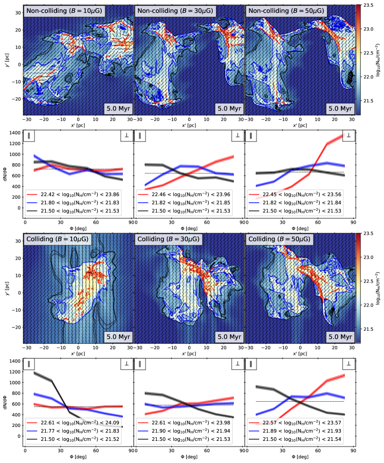
Figure 2: First and third rows: Column density maps with the normalized plane-of-sky magnetic polarization field, $p$, represented with black pseudo-vectors. The non-colliding cases for $B=10$, 30 and 50 $\mu$G are shown in the first row, while the respective colliding cases are shown in the third row. Gas from the density regulated SF models are shown in each case at $t=5\>{\rm Myr}$. Second and fourth rows: Histogram of Relative Orientations (HROs) are shown directly below their corresponding column density maps. HROs compare the angle between $p$ vs. iso-$N_{\rm H}$ contours pixel-by-pixel. The projected map is divided into 25 column density bins of equal pixel count. HROs for the lowest (1st bin; black), middle (12th bin; blue), and highest (25th bin; red) $N_{\rm H}$ are shown, using angle bins of $15\degree$. The histogram color corresponds to the regions bounded by low (black), intermediate (blue), and high (red) value iso-$N_{\rm H}$ contours as shown in the respective projection map. The thickness of the data points indicates the variance within each bin. Histograms with peaks at $0\degree$ correspond to $p$ predominantly aligned with iso-$N_{\rm H}$ contours (i.e., $B$-fields parallel to filaments), while peaks at $90\degree$ correspond to $p$ predominantly perpendicular to iso-$N_{\rm H}$ contours (i.e., $B$-fields perpendicular to filaments).

The formation and evolution of filamentary structures in molecular clouds may be strongly affected by the orientation of the $B$-field. Li et al. (2013) observed a bimodal distribution of preferentially parallel and perpendicular orientations between filamentary Gould Belt clouds and their encompassing $B$-fields. They concluded that dynamically important $B$-fields must be present, which both guide the gravitational contractions (perpendicular orientations) and channel turbulence (parallel orientations). If the primary filament formation mechanism were instead super-Alfvénic turbulence there should be no preferential alignment.

Soler et al. (2013) developed a pixel-by-pixel approach to quantify the degree of alignment of magnetic fields with respect to filamentary structures defined by column density gradients. This statistical method, the Histogram of Relative Orientations (HRO), measures the relative orientations for a given (column) density and has since been widely used in both polarization observations (e.g., Planck Collaboration et al., 2016) and numerical simulations (e.g., Planck Collaboration et al., 2015; Chen et al., 2016; Wu et al., 2017b).

For simulations described in the current work, we apply an HRO formulation where

$$\Phi=\left|\arctan\left(\frac{\nabla N_{\rm H}\cdot\bm{p}}{|\nabla N_{\rm H}\times\bm{p}|}\right)\right|$$ (8)

is the magnitude of the angle between $N_{\rm H}$ iso-contours (orthogonal to $\nabla N_{\rm H}$) and $\bm{p}$, the simulated polarization pseudo-vectors. $\bm{p}$ is defined as

$$\bm{p}=(p\sin\chi)\hat{\bm{x}}+(p\cos\chi)\hat{\bm{y}}$$ (9)

where $p=0.1$ is a set constant polarization fraction and $\chi$ is the angle in the plane-of-sky derived from the Stokes parameters (see, e.g., Wu et al., 2017b):

$$q=\int n\frac{B_{y}^{2}-B_{x}^{2}}{B^{2}}ds$$ (10)

$$u=\int n\frac{2B_{x}B_{y}}{B^{2}}ds$$ (11)

$$\chi=\frac{1}{2}\arctan 2(u,q)$$ (12)

The relative orientation angle $\Phi$ is then calculated pixel-by-pixel in a column density map. The lowest column density pixels ($N_{\rm H}<21.5\>{\rm cm^{-2}}$) are ignored and a gradient threshold for $\nabla N_{\rm H}>0.25\overline{N_{\rm H}}$ is applied (similar to, e.g., Planck Collaboration et al., 2016), to better separate GMC material from diffuse background fields. The remaining pixels are then separated into 25 bins of equal count based on $N_{\rm H}$. Note that we assume $n_{\rm He}=0.1\>n_{\rm H}$, yielding a mass of $2.34\times 10^{-24}\>{\rm g}$ per H.

Figure 2 shows column density maps for the non-colliding and colliding models with $B=10$, 30, 50 $\mu$G, respectively, for the density-regulated model. Their respective HROs are also shown, for low, medium, and high column density bins. Here, $\phi$ represents the smaller angle between the polarization-inferred magnetic field and $N_{\rm H}$ iso-contours. Thus, histograms peaking at $\phi=0\degree$ indicate inferred $B$-fields preferentially aligned parallel to filamentary structures, while peaks at $\phi=90\degree$ indicate a preferentially perpendicular alignment.

Gas in the non-colliding, $B=10\>{\rm\mu G}$ model is slightly preferentially aligned parallel to filaments at high, medium, and low column densities. At $30\>{\rm\mu G}$, the low-$N_{\rm H}$ gas retains effectively the same orientation behavior, while the mid- and high-$N_{\rm H}$ bins show an increasing trend toward perpendicular alignment. This trend increases further in the $50\>{\rm\mu G}$ case, where the low-$N_{\rm H}$ gas has random alignment, mid-$N_{\rm H}$ gas has slightly perpendicular alignment, and high-$N_{\rm H}$ gas is strongly perpendicularly aligned with the $B$-fields.

The colliding GMC models exhibit quite different relative orientations. The low-$N_{\rm H}$ gas in the $B=10\mu$G model is strongly aligned parallel to the $B$-fields, due to the large-scale flows reorienting the fields perpendicular to the velocities. The degree of alignment decreases for increasing $N_{\rm H}$ bins, with essentially no preferential alignment for the highest-$N_{\rm H}$ regions. Similar to the non-colliding cases, the alignment of filamentary structures shifts towards more perpendicular relative orientations in higher $B$ environments. However, the lowest-$N_{\rm H}$ structures remain fairly preferentially oriented parallel to the $B$-fields, due to effects of the colliding flows on the ambient gas.

Observationally, HROs from active star-forming regions typically reveal polarization vectors oriented in a preferentially parallel alignment with low-$N_{\rm H}$ gas structures. For high-$N_{\rm H}$ gas structures, there tends to instead be a random or preferentially perpendicular alignment, . From our simulations, distinctive signs of a collision include a strongly parallel alignment of low-density gas, though lower $B$-field non-colliding models also exhibit this behavior but to a lesser extent. In both types of models, the strength of the $B$-field has the greatest impact on forming perpendicular alignments with high-$N_{\rm H}$ gas in the HRO. Overall, the degree of separation for low- and high-$N_{\rm H}$ gas in HROs may act as a supplementary tool to investigate both the large scale dynamics and magnetic field strength of star-forming regions.

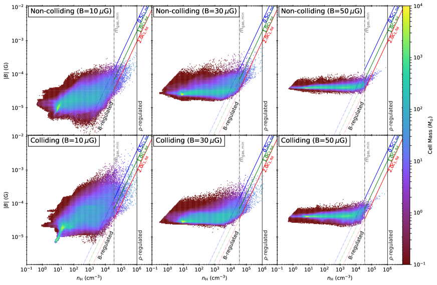
Figure 3: Phase plots of $B$ versus $n_{\rm H}$ for the non-colliding (top row) and colliding (bottom row) cases at 5 Myr. The first, second, and third columns show the $B=10$, 30 and 50 $\mu$G models, respectively, for cell mass distributions using the density regulated SF model. The black vertical line represents the corresponding $n_{\rm H,sf}$ threshold. The blue, green, and red lines represent the various mass-to-flux thresholds for the magnetically-regulated star formation routine. Star particle formation proceeds for densities above these respective limits. The black dash-dot line shows the effective minimum gas density threshold for star formation due to the 50% mass limitation of $m_{\rm\star,min}$ assumed in the sub-grid routines. The Alfvén limiter described in § 2.2 imposes an effective density floor that can be seen in certain models in the low density, higher field strength regimes.

3.2.2 $B$-field Strength vs. Density

Zeeman observations estimating the magnetic field strength with respect to the gas density in the ISM have found a relatively constant value of $B=10\mu$G for $n\lesssim 300\>{\rm cm^{-3}}$ and an approximately power law relation, $B\propto n_{\rm H}^{\kappa}$, above this threshold (Crutcher et al., 2010). The precise value of $\kappa$ has been debated, though indices near $\simeq 0.65$ or 0.5 are estimated, where the former would arise in idealized spherical contraction and the latter from non-isotropic contraction. Mocz et al. (2017) found $\kappa\simeq 0.65$ in their simulations of super-Alfvénic turbulence and $\kappa\simeq 0.5$ for sub-Alfvénic conditions, in agreement with expected gas contraction behavior under weak and strong $B$-fields, respectively.

We investigate the $B$ versus $n_{\rm H}$ relation in our suite of GMC simulations, with the results shown in Figure 3. These phase plots show the total cell mass at each $B$ and $n_{\rm H}$ for the various models, as well as the minimum mass and mass-to-flux thresholds used in the star formation routines.

For the non-colliding case at $B=10\mu$G, a fairly wide range of magnetic field strengths exists for a given density. The peak distribution in gas mass can be attributed to the initially uniform ambient medium. The remaining gas mass generally follows a positive correlation between $B$ and $n_{\rm H}$. In the $30\mu$G model, the overall spread in $B$ is narrower, with an increased average $B$ but similar maximum value. In the $50\mu$G model, the spread in $B$ decreases even further, and the maximum values for both $B$ and $n_{\rm H}$ reached in the simulation are the lowest of the three. As the initial $B$-field strength increases, the overall collapse of the GMCs is strongly inhibited, leading to a more uniform distribution of final $B$-field strength.

The colliding GMC models follow a similar trend where higher global field strengths result in narrower overall distributions in $B$. However, the collisions impart moderately wider spreads in both density and $B$-field strength relative to their non-colliding counterparts. The highest values in both density and $B$-field strength are achieved in the colliding $B=10\mu$G case.

In both scenarios, the effective $\kappa$ index in the $B$ versus $n_{\rm H}$ relation decreases as the average initial $B$-field strength increases. This is consistent with the results found when comparing gas contraction in sub- and super-Alfvénic environments.

Attributes of the star formation routines can be gleaned from these plots as well. Thresholds for the density- and magnetically-regulated models are shown, above which gas will be converted into stars following the methods described in §2.3. For the density-regulated model, this is a simple density threshold. For the magnetically-regulated models, both the mass-to-flux ratios above the respective $c_{1}$ level and the threshold density dictated by $m_{\rm\star,min}$ must be satisfied. The $c_{1}=0.5c_{\rm 1,fid}$ routines yield the greatest total gas mass to be converted into stars in each of the GMC evolution models, resulting in the widest proliferation of star formation as seen in Figure 1. Likewise, models with $c_{1}=2c_{\rm 1,fid}$ generally have less available gas mass and less star formation. However, that which does occur tends to do so in higher density cells at higher mass-to-flux ratios. This leads to different stellar and star-forming gas properties, as detailed in later sections.

3.3 PDFs of Mass Surface Density

Probability distribution functions (PDFs) are a useful statistical tool for connecting gas distributions with the physical mechanisms that shape them. Certain properties of PDFs have been shown in simulations to reveal regimes dominated by turbulence or self-gravity as well as being sensitive to pressure from, e.g., shocks and magnetic fields (Vazquez-Semadeni, 1994; Padoan et al., 1997; Kritsuk et al., 2007; Federrath et al., 2008; Price, 2012; Collins et al., 2012; Burkhart et al., 2015). Observationally, PDFs of mass surface density $\Sigma$ (also $N_{\rm H}$ or $A_{\rm V}$) provide an important link to simulations and have been used to infer underlying physical characteristics of molecular clouds as well as IRDCs (e.g. Kainulainen et al., 2009; Kainulainen & Tan, 2013; Butler et al., 2014).

An area-weighted $\Sigma$-PDF, $p_{A}$, can often be well fit by a lognormal of the form

$$p_{A}(\ln\Sigma^{\prime})=\frac{1}{(2\pi)^{1/2}\sigma_{\ln\Sigma^{\prime}}}\left(\exp{-\frac{(\ln\Sigma^{\prime}-\overline{\ln\Sigma^{\prime}})^{2}}{2\sigma^{2}_{\ln\Sigma^{\prime}}}}\right)$$ (13)

where $\Sigma^{\prime}\equiv\Sigma/\overline{\Sigma_{\rm PDF}}$ is the mean-normalized $\Sigma$ and $\sigma_{\ln\Sigma}$ is the lognormal width, which increases with higher turbulent Mach numbers. Power-law tails often form at high-$\Sigma$, indicative of the degree of gravitational collapse and correlated with the efficiency of star formation.

Figure 4 shows area-weighted $\Sigma$-PDFs at different evolutionary times in non-colliding and colliding simulations where $B=10$, 30, and 50 $\mu$G. These $(32\>{\rm pc})^{3}$ regions are centered on the gas density maximum and projected along the $z^{\prime}$-direction.

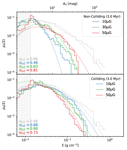
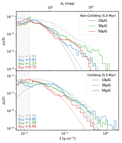
Figure 4: Area-weighted $\Sigma$-PDFs of $(32\>{\rm pc})^{3}$ regions from non-colliding (top panels) and colliding (bottom panels) simulations for $t$=3.0 (left column) and 5.0 Myr (right column). For each case, gas distributions are shown for the $B=10$, 30, and 50 $\mu$G models with density-regulated star formation. In the same color, lognormal fits for each case are plotted as dash-dotted lines and the corresponding width $\sigma_{\ln\Sigma}$ is shown. Also displayed in each panel is the observed $\Sigma$-PDF for the massive IRDC from Lim et al. (2016). The shaded region denotes areas of $A_{V}<3\>{\rm mag}$ corresponding to the lowest closed contour level of the observational data: distributions are only fit above this level.

At $t=3\>{\rm Myr}$, gas distributions in the non-colliding models peak at approximately $0.2\>{\rm g~{}cm^{-2}}$, with weaker initial $B$-fields corresponding to a relatively lower distribution of gas at high $\Sigma$ values. Colliding models reach higher values of $\Sigma$ by the same evolutionary time, with weaker $B$-field models experiencing higher relative increases. This results in a slight reversal of the trend, where collisions in weaker $B$-fields create slightly greater concentrations of material at higher $\Sigma$. The $\sigma_{\ln\Sigma^{\prime}}$ values for the colliding models are greater, on average, and, especially for the more evolved case at 5 Myr, are a closer match to the $\Sigma$ distribution observed in the massive IRDC by Lim et al. (2016).

The gas develops much higher distributions of gas at high-$\Sigma$ in all cases by $t=5\>{\rm Myr}$. Gas exceeds $0.5\>{\rm g~{}cm^{-2}}$ in both the non-colliding and colliding cases, and develops distinct high-$\Sigma$ material not well-fit by the lognormals. The $10\>\mu$G colliding run exceeds $1.0\>{\rm g~{}cm^{-2}}$, while the maximum surface density decreases as initial $B$-field strengths increase. The non-colliding models do not appear to exhibit strong trends based on $B$-field strength. Here, $\sigma_{\ln\Sigma^{\prime}}$ reaches higher values in all cases, with the colliding models generally exhibiting larger widths.

Overall, the $\Sigma$-PDFs reveal that generally greater amounts of high-$\Sigma$ gas form in collisions, while the strength of the $B$-field does not appear to play a large role in shaping the resulting PDFs. The greatest changes in surface density distributions occur with time-evolution, pulling higher concentrations of gas toward the high-$\Sigma$ end and signifying the dominant role of gravity at later stages.

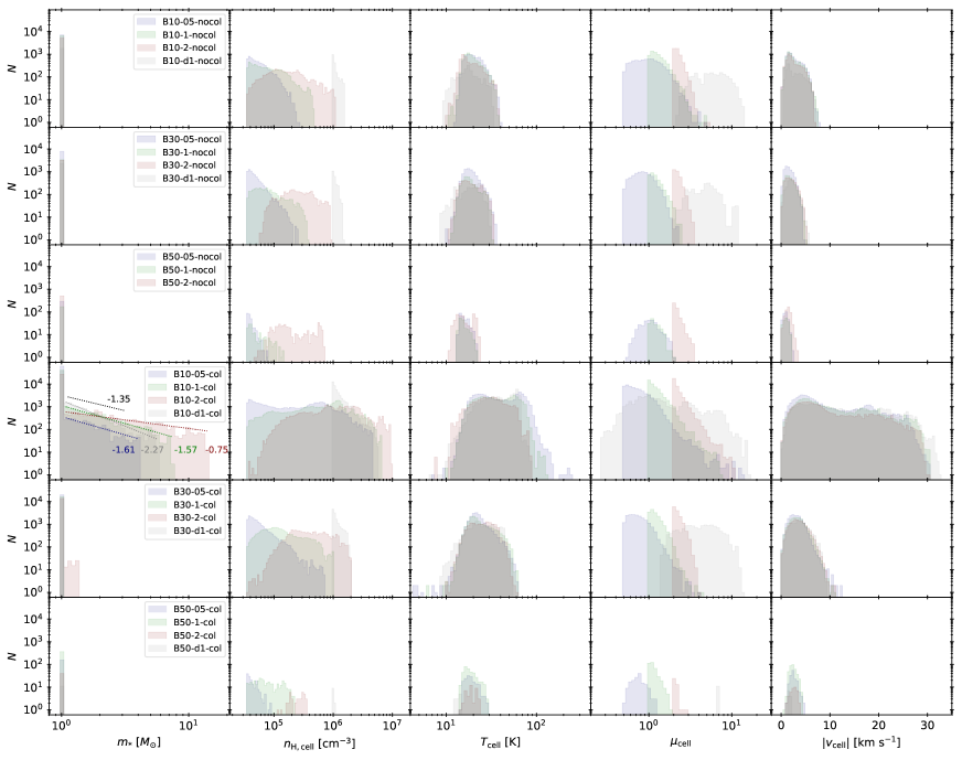
Figure 5: Masses of star particles and properties of star-forming gas cells at the time of star particle creation. (Left to right :) Cumulative histograms for each simulation up to $t=5$ Myr of star particle mass (bin width is 0.03 dex), cell Hydrogen number density (bin width is 0.03 dex), cell gas temperature (bin width is 0.03 dex), cell normalized mass-to-flux ratio (bin width is 0.03 dex), and cell velocity magnitude (bin width is 0.45 km/s) are plotted. The non-colliding (top three rows) and colliding (bottom three rows) cases are shown, for $B=10$, 30, and 50 $\mu$G, respectively. For each case, the results from the density regulated SF routine is shown in gray, while the magnetically regulated SF routines with $c_{1}=0.5,1$ and $2c_{\rm 1,fid}$ are displayed in blue, green, and red, respectively. also include power law fits for the distribution of stars with $m_{\star}>1~{}M_{\odot}$. The power law indices are displayed, as well as a reference -1.35 (Salpeter) index.

3.4 Properties of Star-Forming Gas

We investigate stellar masses and their natal gas properties at the time of star birth, which can be considered to be an approximate representation of the properties of pre-stellar cores in these models, with the caveat that the finest grid resolution is a relatively large 0.125 pc. Figure 5 plots the cumulative histograms for each model, through 5 Myr, of initial star particle masses and progenitor cell gas densities, temperatures, mass-to-flux ratios, and velocity magnitudes in the global center-of-mass frame.

In the non-colliding models, all stars form at the threshold mass of $m_{\rm\star,min}=1~{}M_{\odot}$. This indicates that star formation occurs solely in the stochastic regime of the models, i.e., all stars would have formed with $m_{\star}\leq 1~{}M_{\odot}$. A total number approaching $10^{4}$ are created in the $10\mu$G models, with stronger $B$-fields leading to more than a factor of 10 lower overall star formation.

For star-forming cells in the non-colliding models, the ranges of densities, temperatures, mass-to-flux ratios, and velocities also decrease for higher $B$-field models. As outlined in §3.2.2, the stronger $B$-fields tend to constrain the overall variance in gas density, which is generally correlated with the other properties. For the density-regulated star formation model, no stars are created in the $50\mu$G case, i.e., no cells achieve the threshold density of $n_{\rm H}=10^{6}\>{\rm cm}^{-3}$. For the other cases, star-forming cells lie near the density threshold, while in general, $\mu_{\rm cell}>2$. The magnetically-regulated models form stars in all cases. The $c_{1}$ critical mass-to-flux ratio strongly affects the cell density distribution, but is essentially independent from the cell temperature and velocity.

Star formation occurs in a markedly different manner for the colliding GMC models. In all $10\mu$G cases, a significant number of stars form outside the stochastic regime, representing the occurrence of higher-mass star formation. Following Equation 6, this requires the natal gas cells to accumulate large masses within short timescales. The maximum stellar mass ranges from 4 $M_{\odot}$ in the $0.5c_{\rm 1,fid}$ model to 14 $M_{\odot}$ in the $2c_{\rm 1,fid}$ model. While a fewer total number of stars form with the $2c_{\rm 1,fid}$ model, higher stellar masses are achieved. This can be understood by the higher local mass-to-flux ratio required to initiate star formation, thus enabling cells to reach higher densities just prior to birth of the star.

We fit power laws to these higher-mass stellar distributions, finding indices of -2.27 for the density-regulated model and -1.61, -1.57 and -0.75 for $c_{1}=0.5,1$ and $2c_{\rm 1,fid}$, respectively. The density-regulated model is steeper than the reference -1.35 index, often adopted for the observed IMF (see, e.g., Salpeter, 1955), while the magnetically-regulated models have a range of values that are closer to the Salpeter index, with the higher mass-to-flux ratio threshold leading to the most top-heavy IMF. While other factors that are not yet included, especially protostellar outflows and other forms of feedback may affect the IMF, in the context of our star formation sub-grid models, we see that collisions of relatively weakly magnetized GMCs enable the formation of more massive stars by allowing the rapid accumulation of mass into cells at rates that are faster than can be removed by formation of low-mass stars.

In the higher magnetization colliding models, only the $2c_{\rm 1,fid}$ SF routine for $30\mu$G produces stars with masses above the stochastic regime. Otherwise, they follow a similar trend as the non-colliding cases, with stronger $B$-fields inhibiting overall star formation.

The cells in which stars form exhibit much greater variance in gas properties due to the collisions. In the $10\mu$G cases, the star-forming cells reach densities up to 10 times greater than their non-colliding counterparts. Mean temperatures, mass-to-flux ratios, and velocity magnitudes also increase, as do their variances. The strength of the initial $B$-field plays a large role in the resulting properties found in star-forming gas, with higher $B$-fields constraining the range of the gas properties shown. Differences arising from the collision become much less pronounced in the presence of stronger initial $B$-fields.

The distributions of velocity are closely correlated with the velocity dispersions of the primary clusters (§3.6) in the colliding models. This indicates that a significant fraction of the stars form in the potential of the primary cluster. The weaker correlations for the non-colliding cases are in line with their more dispersed cluster formation, where no single primary cluster dominates the stellar dynamics.

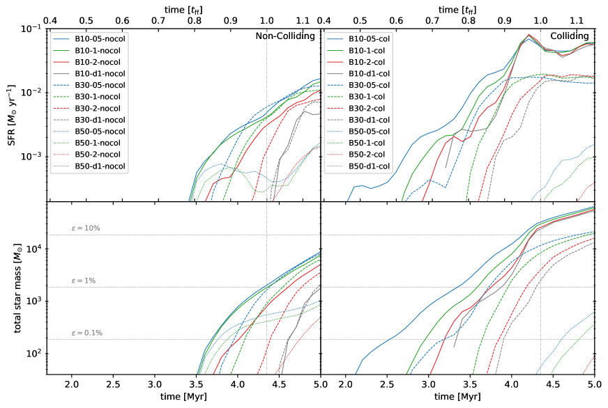
Figure 6: Top row: Star formation rates as a function of time. The non-colliding cases are shown in the left panels, while the colliding models are shown in the right panels. Simulations with $B=10$, 30 and $50\mu$G are shown with solid, dashed and dotted lines, respectively. The density-regulated SF routine is shown in gray, while the magnetically-regulated SF routines with $c_{1}=0.5,1$ and $2c_{\rm 1,fid}$ are displayed in blue, green and red, respectively. The time is shown in both simulation time (bottom axis) and free-fall times of the initial GMCs (top axis). The vertical dotted line indicates one initial free-fall time, i.e., $t_{\rm ff}=4.35$ Myr. Bottom row: The cumulative mass of created stars over time. The star formation efficiency, with reference values shown for $\epsilon$=0.1%, 1% and 10%, is normalized relative to the total initial mass of the two GMCs ($1.86\times 10^{5}\>M_{\odot}$).

3.5 Star Formation Rates and Efficiencies

We next investigate how GMC collisions and $B$-field strength affect the overall SFR and SFE. Figure 6 shows the SFR and cumulative mass of formed stars for each model as a function of simulation time and freefall time of the initial GMCs. The value for SFR at a given time is calculated as the time derivative of the total star mass. Levels for SFE are shown as the total star mass normalized by the combined gas mass of the original two GMCs.

In the non-colliding models, star formation is initiated around $t=3.5~{}$Myr at the earliest, and then showing a general increase in SFR over the course of the simulation. The density-regulated models begin forming stars only after 1 $t_{\rm ff}$, with almost identical behavior for the 10 and $30\mu$G cases, while no stars form in the $50\mu$G case. In the magnetically-regulated models, reduced $c_{\rm 1}$ thresholds lead to earlier star formation, higher SFRs, and higher SFEs. For the $10\mu$G case, SFRs reach $\sim 5\times 10^{-3}\>M_{\odot}\>{\rm yr^{-1}}$ with a SFE of 1% by $t_{\rm ff}$. Stronger field strengths lead to lower overall SFRs and SFEs.

Star formation commences in the colliding GMCs at roughly 2.5, 3.2, and 4.5 Myr for $B=10$, 30 and $50\mu$G, respectively. Within each $B$-field case, as the SF model changes from $c_{\rm 1}$=0.5, 1.0, 2.0, to density-regulated, star formation begins later, SFRs are lower, and SFEs are lower. In all cases, SFEs increase monotonically, while SFRs increase and then begin to level off. The SFRs in the 10 and $30\mu$G cases reach approximately $7\times 10^{-2}$ and $2\times 10^{-2}~{}M_{\odot}\>{\rm yr^{-1}}$, respectively. In the $50\mu$G case, stars only begin to form at $t=5~{}$Myr for the density-regulated model. Overall, star formation efficiencies per freefall time are approximately 15%, 2-5% and 0%, respectively as magnetic field strength increases.

Relative to the non-colliding models, the collision triggers earlier star formation by 1 Myr and enhances SFRs and SFEs by over a factor of 10 in the weaker $B$-field cases. However, as $B$ increases, the enhancement of star formation activity due to collisions is less prominent, and, in the case of $50\mu$G, actually inhibited. This behavior can be attributed to the higher magnetic pressure especially in the bounding atomic regions that lead to a dampening of the collision. The collision cannot efficiently accumulate gas into dense clumps as the magnetic pressure acts to inhibit the flow of gas toward any converging region. These results may be applicable to regions with high densities, magnetic field strengths, and turbulence, yet relatively low SFRs, such as the Central Molecular Zone (e.g., Kruijssen et al., 2014), including the “Brick” IRDC (e.g., Henshaw et al., 2019). However, equivalent simulations for these higher density conditions would need to be carried out to confirm this hypothesis.

The near-convergence of the different star formation models at lower $B$-field strengths indicate that the SFR and SFE are not significantly limited by the density and mass-to-flux thresholds set by our simulations (see also Paper III). Instead, they seem to be determined by the creation of larger structures that contain gas with values greater than the thresholds, which are then converted efficiently into stars even with the $\epsilon_{\rm ff}=0.02$ rate within the star-forming cells. As the $B$-field strength increases, variations among the SF models lead to divergence of the SFRs and SFEs.

Note that in each of these star formation models, key stellar feedback processes such as protostellar outflows, ionization, winds, and radiation pressure have not yet been implemented. While the presented simulations may approximate the initial onset of star formation, the aforementioned feedback mechanisms will likely reduce SFRs at later times.

3.6 Spatial Clustering and Dynamics of Primary Cluster

We investigate how the spatial clustering of stars changes with magnetic field strength and in the presence of collisions. To analyze the overall clustering behavior over the entire GMC complex, we use the minimum spanning tree (MST) which can determine the degree of centrally concentrated clustering versus multi-scale clustering. The substructure within the most massive cluster is explored using the angular dispersion parameter (ADP), a metric that is sensitive to azimuthal variations for chosen radii. Additionally, we calculate the virial parameter to estimate the dynamical state of the primary cluster.

The primary star cluster is found via the popular data clustering algorithm, density-based spatial clustering of applications with noise (DBSCAN) (Ester et al., 1996). DBSCAN defines clusters based on groupings of points with many nearby neighbors and ignores outliers with neighbors that are too far away. Here, we set the points to be our projected star particle locations and set the recovered cluster with the largest population as our primary cluster. To find the center of this cluster, we follow the iterative method introduced in Paper III. First, the median position of the set of cluster members is used as an initial guess. Then, we center on this position a circular aperture with an initial radius of 0.4 pc, and determine a new center based on the center of mass using stars only within this aperture. We repeat this process while iteratively halving the aperture radius until it reaches 0.1 pc. This final defined center is used in the subsequent analysis.

3.6.1 Minimum Spanning Tree

The MST is a graph theory technique which seeks to minimize the lengths of the “edges” that connect all “vertices” of a connected, undirected graph. It was first developed for astrophysical applications by Barrow et al. (1985), and enables the quantitative study of hierarchical substructure of stellar distributions by setting the edge weights to be projected euclidean distances between individual stars.

Cartwright & Whitworth (2004) introduced the $\mathcal{Q}$ parameter to measure the degree of radial concentration in clustering. This is given by

$$\mathcal{Q}=\frac{\overline{m}}{\overline{s}}$$ (14)

where $\overline{m}$ is the normalized mean edge length and $\overline{s}$ is the normalized correlation length, given by:

$$\overline{m}=\sum^{N_{\star}-1}_{i=1}\frac{e_{i}}{\sqrt{N_{\star}A}}$$ (15)

and

$$\overline{s}=\frac{\overline{d}}{R_{\rm cl}},$$ (16)

respectively. $N_{\star}$ is the total number of star particles, $e_{i}$ is the length of each edge (of which there are $N_{\star}$-1), and $A=\pi R_{\rm cl}$ is the cluster area. $R_{\rm cl}$ is distance from the mean star positions to the farthest star, and $\overline{d}$ is the mean pairwise separation distance between the stars. These are discussed in more detail in Wu et al. (2017a) .

A threshold value $\mathcal{Q}_{0}=0.8$ separates star clusters in more centrally condensed associations ($\mathcal{Q}>\mathcal{Q}_{0}$) and those in more substructured, multi-scale associations ($\mathcal{Q}<\mathcal{Q}_{0}$).

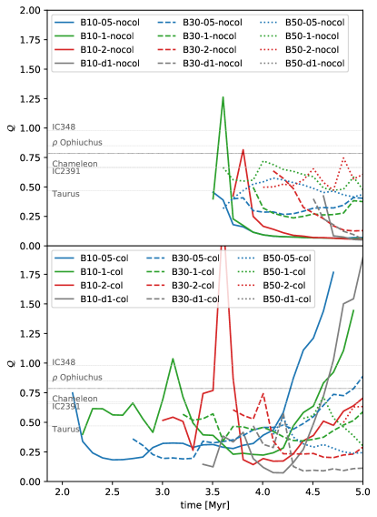
Figure 7: MST $\mathcal{Q}$ parameter versus time. The evolution of $\mathcal{Q}$ is shown for select non-colliding (top) and colliding (bottom) models. Line colors represent different SF models while line styles represent different magnetic field strengths. The values of $\mathcal{Q}$ are averaged over three cardinal lines of sight in the simulation: $x$, $y$, and $z$. The dotted black line denotes the threshold of $\mathcal{Q}_{0}=0.8$ separating smooth radial versus multi-scale clustering. The gray dashed lines show values of $\mathcal{Q}$-parameters of various observed star clusters from Cartwright & Whitworth (2004).

Figure 7 shows the evolution of $\mathcal{Q}$ over time. The non-colliding models show a general trend toward more multi-scale clustering over time. This is consistent with the additional star clusters forming throughout different regions in the GMC complex over time, resulting in a very decentralized overall distribution of stars. As the strength of the $B$-field is increased, the cluster distribution becomes less substructured as star formation occurs in less physically separated regions. Thus, the $\mathcal{Q}$ parameter significantly increases with $B$-field, though it remains under the $\mathcal{Q}_{0}$ threshold for all non-colliding models.

The colliding models reach higher $\mathcal{Q}$ values than their non-colliding counterparts, often placing them within the range of observed star-forming regions. However, after approximately $t=4.5\>{\rm Myr}$, the dominant cluster in the $B=10\>{\mu G}$ colliding models tends become more and more centrally condensed, yielding values up to $\mathcal{Q}\sim 2$. This behavior may largely be due to the lack of stellar feedback, which should limit the production of additional stars within the cluster potential and likely produce less gravitationally bound systems that may have smaller values of $\mathcal{Q}$. The 30 and $50\>{\mu G}$ models show less fluctuation in the degree of clustering, with higher $B$-fields generally yielding higher $\mathcal{Q}$. Sharp maxima in $\mathcal{Q}$ are correlated with increases in the SFR, as new star particles are rapidly created in nearby simulation cells. The inclusion of star particles outside of the main cluster decrease $\mathcal{Q}$.

3.6.2 Angular Dispersion Parameter

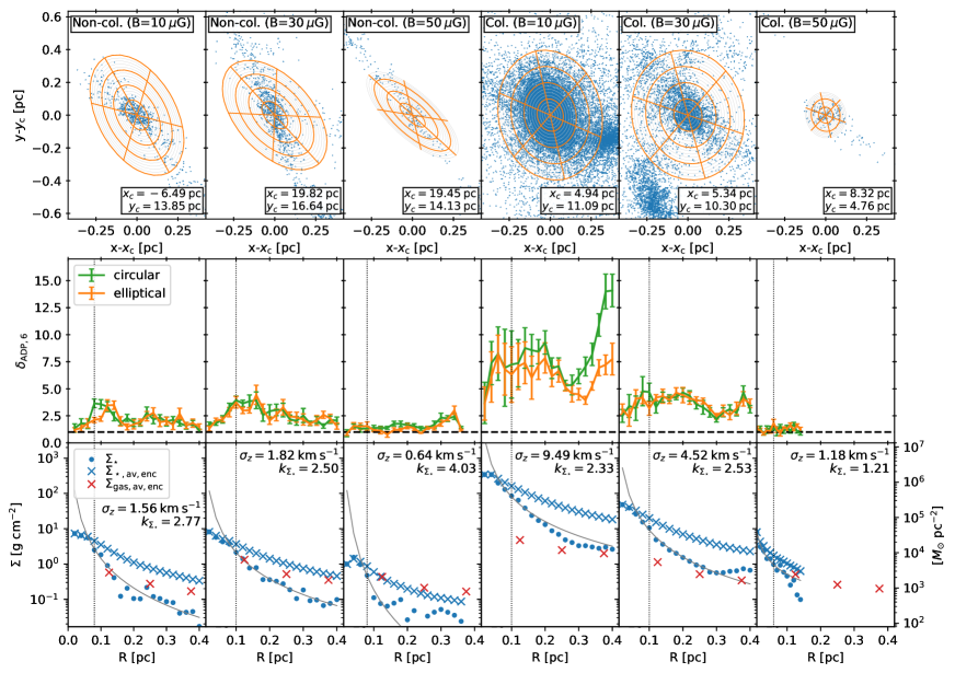
Figure 8: Top row: The primary cluster in each magnetically-regulated star formation simulation at $t=5.0$ Myr as defined by DBSCAN. Blue points denote the projected positions of the star particles, all shown on the same scale and centered iteratively, with final coordinates displayed. The elliptical annuli used to calculate the ADP, $\delta_{\rm ADP,N}$, are drawn in gray, with every fifth annulus and sector division drawn in orange for clarity. Note that no circular annuli are drawn, though they are still used in one version of $\delta_{\rm ADP,6}$ and the radial profiles, both described below. Middle row: $\delta_{\rm ADP,6}$ versus radius from the cluster center. Values are calculated using both the circular (green) and elliptical (orange) annuli and averaged over twenty $3\degree$ rotations of the 6-sector pattern. The standard error of the mean is shown by the error bars. The dashed line at $\delta_{\rm ADP,6}=1$ represents a purely random azimuthal distribution of particles (i.e., Poisson). Bottom row: Stellar and gas mass surface densities as a function of radius from each primary cluster center. The stellar profile is shown in blue, with $\Sigma_{\star}$ calculated locally only within each circular annulus and $\Sigma_{\rm\star,av,enc}$ showing the enclosed average quantity. The gray solid line represents a power law fit to $\Sigma_{\star}$ with exponent $k_{\Sigma_{\star}}$ given. The black dotted line denotes the stellar half-mass radius, $R_{1/2}$. The red crosses indicate the average enclosed gas mass, $\Sigma_{\rm gas,av,enc}$. The 1-D velocity dispersion of the stars, $\sigma_{z,1/2}$, is calculated for the cluster as defined by the half-mass radius.

The ADP, $\delta_{\rm ADP,N}(R)$ (Da Rio et al., 2014), is a method that specializes in quantifying the degree of substructure within a stellar cluster. It is sensitive to variations in projected cluster surface density in both the azimuthal and radial directions. This method begins by first spatially dividing the distribution of points among $N$ circular (or elliptical) sectors of equal area. The dispersion of the number of particles contained within each sector is calculated, where values near unity for $\delta_{\rm ADP,N}$ indicate random azimuthal distribution, while higher values of $\delta_{\rm ADP,N}$ correspond to more non-uniform, sub-clustered distributions. Radial dependence can be studied by adding divisions with concentric annuli. We adopt the best-fitted elliptical annuli to account for global eccentricity of the cluster using methods identical to those of Paper III.

The ADP is defined to be

$$\delta_{\rm ADP,N}=\sqrt{\frac{1}{\left(N-1\right)\overline{n}}\sum^{N}_{i=1}\left(n_{i}-\overline{n}\right)^{2}}=\sqrt{\frac{\sigma^{2}}{\sigma^{2}_{\rm Poisson}}}$$ (17)

for an annulus that is divided into $N$ equal sectors, where $n_{i}$ stars are contained within each $i$th sector. $\overline{n}$ is the average number of stars per sector within the annulus, $\sigma$ is the standard deviation of the set of $n_{i}$, and $\sigma_{\rm Poisson}$ is the standard deviation of a Poisson distribution.

In this work, we calculate $\delta_{\rm ADP,N}$ in the primary cluster for each non-colliding and colliding simulation ($B=10$, 30, 50 ${\rm\mu G}$) using the magnetically-regulated star formation model with $c_{1}=c_{\rm 1,fid}$. Figure 8 shows results from both circular and elliptical annuli centered at the iteratively determined cluster center. We use $N=6$ sectors and typically 20 equally-spaced concentric annuli out to a maximum radius of 0.4 pc. For the 50 ${\rm\mu G}$ non-colliding and colliding cases, respectively, we use 18 annuli out to 0.36 pc and 14 annuli out to 0.14 pc due to the smaller cluster extents and lower stellar densities formed in these models. The dispersion is calculated twenty times using sector patterns rotated every $3\degree$ and averaged to obtain $\delta_{\rm ADP,6}$.

Immediately evident is the difference in sizes and distributions of the most massive cluster formed from quiescent evolution in a non-collision case compared to those formed in a GMC-GMC collision. The non-colliding models form relatively elongated primary clusters along gas filamentary structures, with only a slight drop-off in membership as the global initial $B$-field increases. On the other hand, the primary clusters in the colliding models exhibit more complex substructure in a more crowded environment and experience large decreases in population as the $B$-field increases.

The ADP as calculated from circular and elliptical annuli do not differ greatly as functions of radii. $\delta_{\rm ADP,6}$ for each of the non-colliding models behaves near Poisson at the center, then increases to moderate levels of dispersion. The $50\>{\rm\mu G}$ case shows lesser degrees of dispersion.

In the $10\>{\rm\mu G}$ colliding case, $\delta_{\rm ADP,6}\simeq 7.5$, indicating a much higher degree of angular dispersion, especially when a secondary cluster is incorporated near $R=0.4\>{\rm pc}$. Clusters in the higher $B$-field cases show lower levels of dispersion.

The primary clusters formed in the non-colliding models and the more strongly magnetized colliding models in fact exhibit similar ADP values as the ONC, where $\delta_{\rm ADP,6}\simeq 2$ (Da Rio et al., 2014). The $10\>{\rm\mu G}$ colliding case forms a primary cluster with much higher ADP. Implementing various forms of local feedback should work to lower the degree of substructure in each scenario, and the ADP method of quantifying cluster substructure may be a useful test of such effects.

3.6.3 Dynamical State of Primary Cluster

The bottom row of Figure 8 shows stellar and gas mass surface densities as functions of radius. Note that only circular annuli are used in this analysis. $\Sigma_{\star}$ shows the mass surface density of stars within each annulus, $\Sigma_{\rm\star,av,enc}$ shows the enclosed average quantity at a given radius, while $\Sigma_{\rm gas,av,enc}$ represents the enclosed average quantity for gas.

The non-colliding models have relatively similar radial profiles, with $\Sigma_{\rm gas,av,enc}$ similar to $\Sigma_{\rm\star,av,enc}$ at $\sim 1-10\>{\rm g\>cm^{-2}}$ near the cluster center and decreasing at greater radii. As the global magnetic field is increased, the mass surface densities decrease, though the fraction of gas to star mass surface density increases. This can be explained by the corresponding decrease in level of star formation activity.

Much higher star formation activity is present in the colliding models, which explains the $\sim 1-2$ orders of magnitude higher mass surface densities. In these cases, $\Sigma_{\rm\star,av,enc}$ exceeds $\Sigma_{\rm gas,av,enc}$ significantly, i.e., achieving much higher local star formation efficiencies.

A power law is fit to $\Sigma_{\rm\star}$,

$$\Sigma_{\rm\star}(R)\propto\left(\frac{R}{0.2\>{\rm pc}}\right)^{-k_{\sigma_{\star}}},$$ (18)

where $R$ is the radius from the cluster center and $k_{\sigma_{\star}}$ is the power law index. This index is generally about 2.5 in the primary clusters, but varies for more irregular clusters formed in the $50\>{\rm\mu G}$ models.

The half-mass radius, $R_{1/2}$, is defined as the radius within which half of the total cluster mass from the maximum aperture radius (typically 0.4 pc) is contained. $R_{1/2}$ is generally near 0.1 pc for the primary clusters. The stellar masses contained within $R_{1/2}$ for the non-colliding models are $4.0\times 10^{2}$, $5.5\times 10^{2}$, and $8.4\times 10^{1}\>{M_{\odot}}$, respectively, for $B=10$, 30, and $50\>{\rm\mu G}$. For the respective colliding models, they are $2.2\times 10^{4}$, $2.7\times 10^{3}$, and $9.2\times 10^{1}\>{M_{\odot}}$. The clusters formed in a collision have a much stronger dependence on the global magnetic environment compared with those formed in non-colliding models.

Stellar mass surface densities estimated within observed clusters of similar mass $M_{\star,1/2}\lesssim 1.0\times 10^{3}\>M_{\odot}$ are generally lower than those found in these simulations (Tan et al., 2014), except for the strongest magnetization cases. Again, this may be explained by the lack of stellar feedback in our simulations and is expected to better match observations when protostellar outflow and radiative feedback mechanisms are implemented.

The dynamical state of a cluster can be estimated using the virial ratio,

$$Q=-\frac{T_{\star}}{\Omega}=\frac{3\sigma^{2}R}{2GM_{\star}},$$ (19)

where the total kinetic and gravitational potential energies of the stars are given by $T_{\star}$ and $\Omega$, respectively. $R$ is the radius that contains a total stellar mass of $M_{\star}$ and $\sigma$ is the 1-D velocity dispersion of all enclosed stars. $Q=0.5$ indicates a state of virial equilibrium and values above and below 1 indicate clusters that are gravitationally unbound and bound, respectively. $Q$ can also be related to the virial parameter (Bertoldi & McKee, 1992), commonly defined as

$$\alpha_{\rm vir}=3\left(\frac{5-2n}{3-n}\right)\left(\frac{\sigma^{2}R}{GM}\right),$$ (20)

where $M$ is the total mass enclosed in $R$ and $n$ is the index of the radial density profile, $\rho(r)\propto r^{-n}$. For an $n=2$ profile, this yields a relationship of $Q=0.5\alpha_{\rm vir}$.

At $R_{1/2}$, virial ratios of 0.17, 0.21, and 0.14 are found for the non-colliding primary clusters at $B=10$, 30, 50 ${\rm\mu G}$, respectively. For the colliding primary clusters, respective virial ratios of 0.14, 0.26, and 0.31 are found. These are all sub-virial, though the more highly magnetized colliding cases seem to form primary clusters closer to virial equilibrium.

However, since the half-mass radii can be $\sim 0.1$ pc, which is about the maximum resolution of AMR grid cells and below the scale at which gravity is softened, these results are likely to be affected by poor numerical resolution. Higher resolution studies are needed to investigate the validity of these results.

3.7 Gas and Star Kinematics

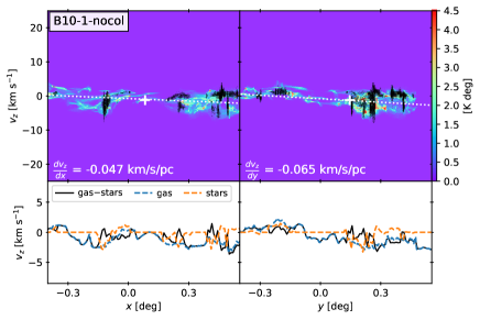
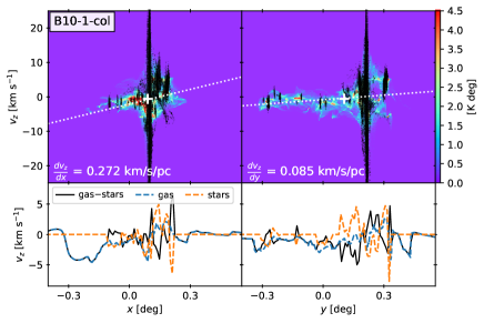
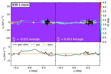
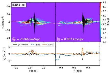
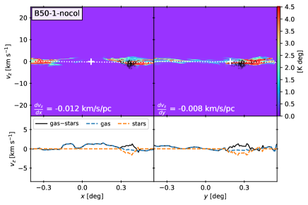
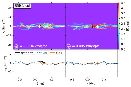
Figure 9: Position-velocity diagrams for non-colliding (left column) and colliding (right column) simulations for the $B=10\>{\rm\mu G}$ (row 1), $30\>{\rm\mu G}$ (row 2), and $50\>{\rm\mu G}$ (row 3) simulations using $c_{1}=c_{\rm 1,fid}$. Each model is shown at $t=5.0\>{\rm Myr}$ along the $z$ line-of-sight. The colormap depicts synthetic ¹³CO($J$=1-0) line intensities from the gas through velocity bins of $\Delta v=0.212\>{\rm km\>s^{-1}}$. The star particles are shown as black points. The gray cross indicates the position of the center of mass and the solid white line shows the intensity-weighted linear velocity gradient ($dv_{\rm los}/ds$) across each cloud. Below each respective position-velocity diagram are plots of the mean gas velocity, mean star velocity, and their difference. Positional bins of $0.5~{}{\rm pc}$ (i.e., $9.5\times 10^{-3}~{}{\rm deg}$ for an adopted system distance of 3 kpc) are used.

Evidence of the formation mechanism of young embedded clusters may remain imprinted shortly after on the kinematics of young stars and their surrounding gas. Position-velocity diagrams have been used to investigate the kinematics of cluster forming environments in simulations and observations (see, e.g., Duarte-Cabral et al., 2011; Dobbs et al., 2015; Butler et al., 2015; Haworth et al., 2015). Radial velocity differences, $\Delta v_{r}$, between young stellar objects and ¹³CO along their line of sight have been analyzed by Da Rio et al. (2017), who found that regions with the greatest differences coincided with the more evolved regions of the cluster.

Using similar procedures as Wu et al. (2017a), Figure 9 compares position-velocity diagrams between non-colliding and colliding models for $B=10$, 30 and $50\mu$G, respectively. The gas represented by synthetic ¹³CO($J$=1-0) emission has velocity resolution of $0.212~{}{\rm km\>s^{-1}}$ and is assumed to be optically thin and located at $d$=3 kpc. Also plotted are the ¹³CO intensity-weighted radial velocities for the gas, mass-weighted radial velocities of the stars, and the difference between the two velocity components.

Gas in the non-colliding models is generally dispersed, with moderate velocity dispersions of a few km/s throughout the various line of sight positions. As $B$ increases, the velocity dispersion of the gas and the stars is reduced. The magnitude of the gas velocity gradient experiences a strong reduction as well. The spatial distribution of stars changes from numerous small, scattered clusters to one primary region of star formation. Velocity differences between gas and stars are generally $\sim 1~{}{\rm km\>s^{-1}}$, with slight fluctuations.

Collisions trigger the creation of more disrupted gas and star kinematics that can be readily seen in position-velocity space. The gas is more concentrated in the collision axis ($x$) due to the large-scale flows and also in the orthogonal axes ($y$ shown here) from the higher gravitational potential of the dense clump. The velocity dispersion of stars and gas is also greatly enhanced, reaching more than $\pm 5~{}{\rm km\>s^{-1}}$ in the $B=10\mu$G case. Cloud collisions also appear to impart higher velocity gradients in the dense clump. Gas and star velocity differences, too, see large fluctuations and magnitudes relative to the non-colliding cases. As $B$ increases, the magnitudes of velocity dispersions, gradients, and differences are all sharply reduced. However, a higher gas velocity dispersion relative to the respective non-colliding cases remains present.

4 Discussion and Conclusions

We have presented MHD simulations to investigate how magnetic field strengths affect the star formation process in self-gravitating, magnetized, turbulent GMCs evolving relatively quiescently compared with identical GMCs undergoing collisions at a relative speed of 10 km/s. $B$-field strengths of $B=10$ (i.e., moderately magnetically supercritical), 30 (i.e., marginally supercritical), and $50\mu$G (i.e., near critical) are explored, with star formation being governed by sub-grid routines regulated by either the gas density or the local mass-to-flux ratio. In such environments, the cloud and cluster morphology, magnetic field orientations and strengths, properties of star-forming gas, star formation rates and efficiencies, and star versus gas kinematics were analyzed.

Stronger $B$-fields are seen to reduce the degree of fragmentation in both non-colliding and colliding cases and significantly alter the collision process due to increased magnetic pressure in the intervening material. The resulting number of stars is reduced and distributed among fewer clusters.

The relative orientations between filamentary structures and $B$-fields become increasingly preferentially perpendicular in the presence of stronger $B$-fields, . This effect is seen most prominently in higher column density regions. In low column density regions, there exists approximately random relative orientations in the non-colliding models, while the collision forms preferentially parallel orientations. Weaker global fields in fact created subregions with the highest $n_{\rm H}$ and strongest $|B|$, while stronger fields limited the overall dispersion in density and $B$-field values.

$\Sigma$-PDFs have imprints of the initial $B$-field strength at early times, where stronger fields form slightly higher-$\Sigma$ distributions in the non-colliding cases, but collisions more greatly enhance the $\Sigma$ of weaker field cases. At later stages in the evolution, some $\Sigma$-PDFs develop structures not well-fit by lognormals.

Stars that formed in the non-colliding models all fell within the $\leq 1M_{\odot}$ regime, and their natal gas exhibited distributions of density, temperature, magnetic criticality and velocity that narrowed as $B$-field strength increased. However, the supercritical colliding models produced a higher dispersion of gas properties, with the $10\mu$G model in particular forming stars with a distribution of higher masses in approximate agreement with a power law distribution, $dN/d\>{\rm log}m_{*}^{\alpha_{*}}$ with index $\alpha_{*}=$-1.35.

For $B=10\mu$G, colliding GMCs resulted in a factor of 10 increase in SFR and thus a factor of 10 increase in efficiency relative to the non-colliding counterparts, in agreement with previous studies. However, this enhancement is reduced and even reversed in simulations with stronger global fields, which inhibit the collision and star formation. These results suggest a potential role of cloud collisions in efficiently forming massive star clusters, while lower mass star formation may typically take place in more quiescent or more strongly magnetized environments.

The spatial distribution of star formation, e.g., as measured by the minimum spanning tree $\mathcal{Q}$ parameter, is much more dispersed in the non-colliding cases and much more concentrated, i.e., in a more dominant primary cluster, in the colliding cases. The primary cluster formed within each simulation showed larger sub-structure in the colliding cases. All primary clusters were found to be sub-virial, but the more strongly magnetized colliding cases exhibited clusters closest to virial equilibrium. However, since the half-mass radii can be $\sim 0.1$ pc, which is about the maximum resolution of AMR grid cells and below the scale at which gravity is softened, these results are likely to be affected by numerical under resolution.

Stronger $B$-fields also resulted in reduced velocity dispersions, velocity gradients, and degree of stellar kinematics overall. Such properties were enhanced by the collision in each $B$-field case.

References

- Anathpindika (2009) Anathpindika, S. 2009, A&A, 504, 437
- Balfour et al. (2015) Balfour, S. K., Whitworth, A. P., Hubber, D. A., & Jaffa, S. E. 2015, MNRAS, 453, 2471
- Barrow et al. (1985) Barrow, J. D., Bhavsar, S. P., & Sonoda, D. H. 1985, MNRAS, 216, 17
- Bertoldi & McKee (1992) Bertoldi, F., & McKee, C. F. 1992, ApJ, 395, 140
- Bisbas et al. (2017) Bisbas, T. G., Tanaka, K. E. I., Tan, J. C., Wu, B., & Nakamura, F. 2017, ApJ, 850, 23 (Paper V)
- Blitz & Shu (1980) Blitz, L., & Shu, F. H. 1980, ApJ, 238, 148
- Bryan et al. (2014) Bryan, G. L., Norman, M. L., O’Shea, B. W., et al. 2014, ApJS, 211, 19
- Burkhart et al. (2015) Burkhart, B., Collins, D. C., & Lazarian, A. 2015, ApJ, 808, 48
- Butler et al. (2014) Butler, M. J., Tan, J. C., & Kainulainen, J. 2014, ApJ, 782, L30
- Butler et al. (2015) Butler, M. J., Tan, J. C., & Van Loo, S. 2015, ApJ, 805, 1